Atmospheric CO₂ and CH₄ measurements at Schauinsland station, Germany: a comparative study of diurnal and seasonal variations at 12 and 35 m intake height

At the atmospheric monitoring station Schauinsland (Black Forest, Germany), high-precision long-term measurements of atmospheric CO₂ and CH₄ have been conducted since 1972 and 1991, respectively. An additional air intake at 35 m a.g.l. (above ground level) has been installed alongside the existing intake at 12 m a.g.l. in September 2021. To ensure consistency and continuity of the historic CO₂ and CH₄ time series, a three-year comparison between the two intake heights has been carried out. This revealed systematic differences in CO₂ mole fractions between the two levels: During summer, daytime diurnal mean CO₂ mole fractions at 35 m are up to 0.5 ppm higher, while night-time values are up to 1.1 ppm lower, compared to 12 m, resulting in smaller diurnal amplitudes at 35 m. Seasonal mean CO₂ mole fractions are lowered by up to 0.36 ppm at 35 m relative to 12 m in summer, whereas no significant differences are observed in winter. The diurnal and seasonal mean CH₄ mole fraction differences between the two intake heights are negligible. However, highly frequent CH₄ spikes originating from nearby grazing cows, which are present only during the summer months, increase hourly mean mole fractions at 12 m by up to 38 ppb, while no significant influence is measured at 35 m. The REBS (Robust Extraction of the Baseline Signal) algorithm is applied to the minutely CH₄ summer data at 12 m and proved to be an effective approach for identification of data affected by very local influences.

1 Introduction

Long-term, high precision measurements of atmospheric CO₂ and CH₄ are essential for monitoring and understanding global biogeochemical cycles in the context of ongoing rapid climate change. The observed long-term trends, interannual, diurnal and seasonal variations in atmospheric CO₂ and CH₄ mole fractions derived from continuous in situ measurements, carry the imprint of surface fluxes. For example, recent observations indicate a declining capacity of the land carbon sink in Central Europe between 2014 and 2023, driven by reduced rainfall and elevated temperature due to climate variability and change (Friedlingstein et al., 2025). These land and ocean carbon fluxes are estimated by inverting atmospheric transport models, constrained by data from numerous continental and marine greenhouse gas monitoring station within different observational networks (e.g. WMO, 2025a; Heiskanen et al., 2023; Lan and Dlugokencky, 2024). With a CO₂ record spanning over 54 years, the measurements at Schauinsland station in Germany represents the longest continuous CO₂ time series in Europe. Schauinsland station is located on a mountain ridge at an altitude of about 1000 m above the populated and industrialized Rhine Valley in the Black Forest, surrounded by meadows and forests. Data from Schauinsland station provide valuable information on the biospheric and anthropogenic greenhouse gas emissions in Western Europe (Schmidt et al., 1996, 2001, 2003) and are used in numerous studies (e.g. Bergamaschi et al., 2018; Rödenbeck et al., 2020). Schauinsland station is part of the atmospheric measurement infrastructure of the German Environmental Agency (UBA), the Monitoring and Evaluation Programme (EMEP, Tørseth et al., 2012) and the Global Atmosphere Watch Programme (GAW, WMO, 2025a) and joined the Integrated Carbon Observatory System (ICOS, Heiskanen et al., 2023) network in May 2022.

ICOS is a European high precision network of atmospheric, oceanic and terrestrial measurement sites that standardizes measurement protocols and centralizes data processing (Heiskanen et al., 2023). In line with the World Meteorological Organization Global Atmosphere Watch (WMO/GAW) recommendations, ICOS aims to archive network compatibility targets of 0.1 ppm for CO₂ and 2 ppb for CH₄ (WMO, 2025b; ICOS RI, 2020). Such measurement consistency is critical because seasonal CO₂ gradients between European stations typically amount to only a few parts per million (Ramonet et al., 2010). Even large-scale climatic extremes, such as the severe drought and heatwave affecting Northern and Central Europe in summer 2018, cause a perturbation of the seasonal cycles in the most impacted regions of only 1.4 ppm (Ramonet et al., 2020). Moreover, diurnal variations of CO₂ mole fractions need to be represented correctly, as misrepresentation can introduce substantial bias in flux inversions at continental and regional scales (Munassar et al., 2025). To minimize the influence of local surface fluxes, the relocation of the 12 m air intake line at Schauinsland station to a 35 m high television tower was implemented in 2021. The key concern associated with this change is that differences in intake height may introduce systematic biases in diurnal and seasonal cycles, potentially affecting the interpretation of regional greenhouse gas fluxes.

Beyond systematic differences related to intake height, short-term perturbations caused by local emissions represent an additional challenge for the representativeness of long-term atmospheric background observations. Contamination by local sources has been reported at other atmospheric monitoring sites, such as CO and CO₂ pollution at Zugspitze (ZSF), which can be removed successfully via manual flagging by the station PI (Hoheisel et al., 2023); or CH₄ spikes related to offshore sand dredging activities at the marine station Westerland in the north of Germany (Schmidt el al., 2026a). At the Ispra station in Italy, local pollution related to cattle leads to enhancements of several parts per million in the CH₄ record and has been addressed using the REBS spike detection algorithm (Cristofanelli et al., 2023; Bergamaschi et al., 2022). While such spike detection algorithms are increasingly applied in the community, their optimal configuration depends on the trace gas, station characteristics and the temporal properties of the pollution events (El Yazidi et al., 2018; Cristofanelli et al., 2023).

In this study, we use three years of parallel measurements (2022–2024), to assess the comparability of CO₂ and CH₄ dry air mole fractions, hereafter referred to as mole fraction, measured at 12 and 35 m at Schauinsland station. The new 35 m sampling line is equipped with a dedicated second Cavity Ringdown Spectroscopy (CRDS) analyzer, which enables simultaneous measurements and direct comparisons between the two intake heights. We quantify systematic differences in diurnal and seasonal variability associated with intake height. In addition, we apply an automated spike detection approach to identify and mitigate short-term CH₄ perturbations and evaluate how the new 35 m intake can reduce contamination by local sources. The results provide guidance on integrating the 35 m intake into the long-term CO₂ and CH₄ records at Schauinsland station, thereby ensuring continuity and data quality for Europe's longest-running atmospheric greenhouse gas time series.

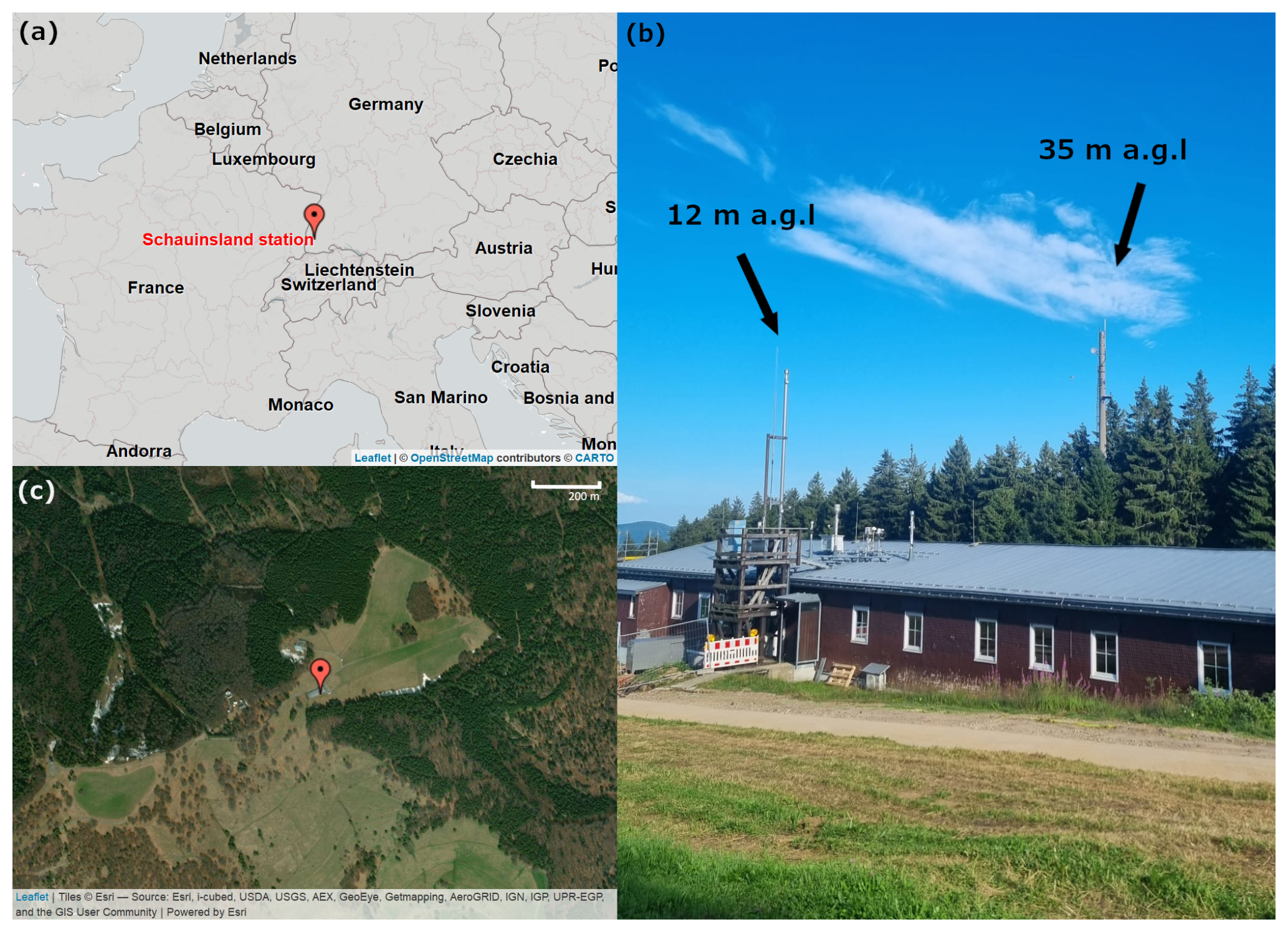
Figure 1 Location of Schauinsland station in central Europe created with Leaflet package for R (a). Photo of the station in summer, highlighting the two air intakes at 12 and 35 m a.g.l. (b). Map showing the surrounding of Schauinsland station (OpenStreetMap) created with the Leaflet package for R (c).

2 Schauinsland station

2.1 Site description

Schauinsland station (47°55 N, 7°55 E) is located in southwest Germany in the Black Forest on the Schauinsland mountain ridge, 1205 m above sea level and approximately 1000 m above the densely populated Rhine valley (Fig. 1a). The area surrounding the station is predominantly characterized by forest and pasture (Fig. 1c). The nearest village is Hofsgrund (300 inhabitants) located 1.5 km from the station. The city of Freiburg with a population of 240 000 lies 8 km northwest from the station in the Rhine valley. The Upper Rhine Plain at an altitude of ∼ 200 m is characterized by cropland and urban areas with the cities of Basel, Mulhouse, Colmar, Strasbourg, Karlsruhe, Mannheim and Ludwigshafen.

The region exhibits a warm temperate climate, fully humid with warm summers and frequent snow cover in winter. The main wind direction is west-southwest. As a mountain station, the summer wind regime shows a pattern of upslope winds during the day and downslope winds at night (Schmidt et al., 1996). The station is usually above the planetary boundary layer (PBL) during the night, but during the day and especially in summer, the PBL can often exceed the height of the station.

2.2 Instrumental setup

In September 2021, a new air intake line was installed at a height of 35 m above ground level (a.g.l.) at a nearby radio tower located approximately 50 m south-east of the station, complementing the routine 12 m air inlet system (Fig. 1b). Since then, the measurement setup has comprised two separate intake lines, each connected to its own CRDS analyzer (G2301, Picarro Inc., Santa Clara, CA, USA). A SynFlex tube with an inner diameter of 10.8 mm is installed from the air intake at the top of the tower to its base and continues underground over a distance of 70 m to the basement of the station, from where the sample air is routed to the analyzer. The corresponding residence times are approximately 13 s for the 35 m tower section at a flow rate of 15 L min⁻¹ and 52 s for the 70 m underground section at a flow rate of 18 L min⁻¹. A refrigeration unit located at the base of the tower pre-dries the air at 2 °C to reduce the moisture content. The routine air inlet located at 12 m a.g.l. supplies several instruments through a glass intake tube with an air flow of 500 L min⁻¹. The CRDS analyzer is connected to this system with a stainless-steel tubing. Both instruments measure the mole fraction of CO₂, CH₄ and H₂O in ambient air with a temporal resolution of 3.6 s (Table 1). The measured H₂O mole fraction is uncalibrated and is used solely as an ancillary quality control parameter. Before entering the CRDS analyzers, the air is dried with a Nafion dryer, following the setup of Welp et al. (2013), which was installed in March 2022 for instrument 529/881 (35 m) and in October 2022 for instrument 1072 (12 m).

Table 1 Chronological overview of CRDS instruments operated at Schauinsland station since 2011.

The measurement setup follows the ICOS guideline for atmospheric measurements (ICOS RI, 2020). Six compressed gas cylinders are used for calibration and quality control: One long-term target or archive gas, one short-term target and four calibration cylinders. They are connected to the three instruments, including a CO $/$ N₂O analyzer (instrument 1074), via one 4-way cross per cylinder and a multi-position valve (EMT2CSD16UWE, Valco Vici, Switzerland) for each analyzer. The calibration and target cylinder measurement sequence are controlled by the valve sequencer of each instrument that commands the respective multi-position valve.

Figure 2 Schematic of the measurement setup with two separate air intake lines.

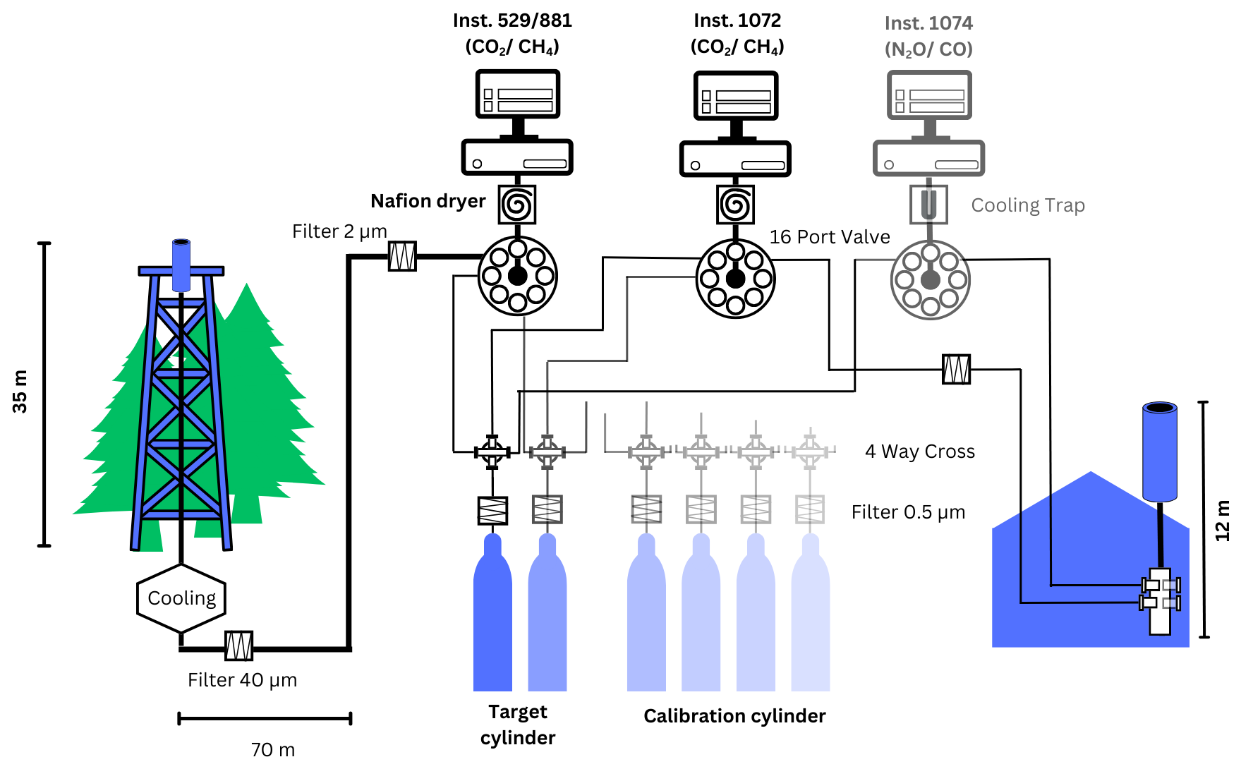
Meteorological parameters like ambient air pressure, temperature and relative humidity are measured about 40 m northeast of the station with a temporal resolution of one minute. Due to construction works, the sensors were moved 150 m west of the station in May 2022. Wind direction and wind speed are measured at the radio tower 35 m a.g.l. at minutely resolution with a sonic anemometer (currently Ultrasonic 2D, THIES, Göttingen). In addition, room air temperature, instrument and flushing pump flow rates are logged. A schematic of the measurement setup including both intake lines is shown in Fig. 2.

2.3 Measurement routine, calibration procedure and quality control

In order to relate the measured CO₂ and CH₄ mole fraction to the World Meteorological Organisation (WMO) scales, reference or calibration gas cylinders are analyzed regularly. Since 2021, the calibration and quality control strategy at Schauinsland station is based on the ICOS protocol (ICOS RI, 2020), which defines the requirements for all measurement sites within the ICOS network (Yver-Kwok et al., 2021). A total of four compressed air cylinders covering the full range of atmospheric CO₂ and CH₄ mole fractions is used for the calibration of both analyzers. The calibration cylinders, as well as the target cylinders, are filled and calibrated by the ICOS Calibration Laboratory (ICOS CAL) against the WMO X2019 CO₂ and the WMO X2004A CH₄ scale (https://gml.noaa.gov/ccl/scales.html, last access: 9 February 2026). Each calibration cylinder is injected for 30 min and four calibration cycles are conducted every 15 d. The traceability and quality of the measurement are maintained through daily analysis of a short-term target (STT) and bi-weekly analysis of a long-term target (LTT). These target cylinders are measured as independent, unknown samples and are not used for instrument calibration. Their measured mole fractions are compared with the nominal values assigned by the ICOS Calibration Laboratory (ICOS CAL). The differences should remain well within the ICOS network comparability goals and show neither significant temporal drifts nor step changes, particularly after changes to the calibration cylinders or measurement setup (Yver-Kwok et al., 2021). Additionally, shelter tests are carried out every 6 months to verify that there are no leakages in the intake lines. All raw data are transferred daily to the ICOS Atmospheric Thematic Centre (ATC), where they are processed following the ICOS harmonized methodology (Hazan et al., 2016). After the ICOS data processing, the station manager performs the quality control by reviewing the data in conjunction with the station logbook and flagging periods affected by maintenance, contamination, or other documented technical issues (Hazan et al., 2016; Yver-Kwok et al., 2021).

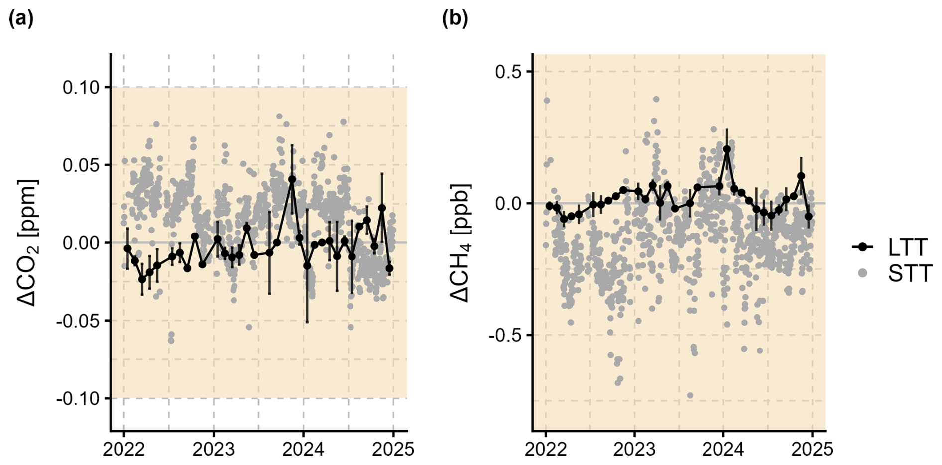
Figure 3 Difference in CO₂ (a) and CH₄ mole fractions (b) measured by instrument 1072 and instrument 529/881 between 2022 and 2024 (1072–529/881). The daily mean CO₂ and CH₄ mole fraction differences of the short-term target (STT) is shown in gray and the monthly mean CO₂ and CH₄ mole fraction differences of the long-term target (LTT) in black. The WMO/GAW compatibility goal of 0.1 ppm for CO₂ and 2 ppb for CH₄ is indicated in beige.

2.4 Comparison of CO₂ and CH₄ target measurements from the two analyzers

Figure 3 shows the comparison of the short-term target (STT) and long-term target (LTT) measurements from the two CRDS analyzers. The difference in CO₂ and CH₄ mole fraction of the target cylinders measured by the instruments 1072 and 529/881 is given as 1072–529/881. The STT (gray) is measured twice a day and averaged to daily mean values, while the LTT (black) is measured once or two times per month and averaged to monthly mean values. The CO₂ measurements from the two analyzers agree well, with mean differences of 0.014 ± 0.023 ppm (mean ±1 standard deviation) for the STT and $-\mathrm{0.003}\pm$ 0.013 ppm for the LTT (Fig. 3a). CH₄ measurements (Fig. 3b) also show no significant discrepancies, with mean differences of $-\mathrm{0.13}\pm$ 0.15 ppb (STT) and smaller than 0.0005 ± 0.0997 ppb (LTT).

2.5 Data treatment

To account for the difference in residence time between the two intake lines, which is approximately 1 min, the minutely data from the two intake systems were first synchronized in time. The synchronized data were then aggregated to hourly means. To derive diurnal cycles for each season, monthly mean diurnal cycles were calculated from hourly CO₂ and CH₄ data. The months were then grouped into seasons according to similar patterns associated with the topographical location of the station: Spring (April and May), summer (June, July, August and September), autumn (October and November) and winter (December, January, February and March). The mean seasonal cycles (annual amplitudes) of the CO₂ and CH₄ time series at Schauinsland station are calculated by first averaging the hourly data to daily means, then to monthly means and finally averaging the monthly means over the three available years. In addition to a seasonal cycle based on all hours of the day, a seasonal cycle based only on daytime data (07:00 to 15:00 UTC) and a seasonal cycle based only on night-time data (21:00 to 05:00 UTC) is calculated. A daily mean is only calculated if at least 12 h means are available (4 h means in case of day or night only). The CO₂ and CH₄ mole fraction difference between the two intake heights of 12 and 35 m is calculated from hourly data and then averaged as above. As no significant difference in the long-term trends between the 12 and 35 m intake heights is expected, the long-term trend is expected to largely cancel out when calculating the difference between the two intake heights. Since the subsequent analysis is based on these intake-height differences rather than on absolute mole fractions, the long-term trend is not expected to significantly affect the results.

2.6 Robust Extraction of Baseline Signal (REBS) spike detection algorithm

The Robust Extraction of Baseline Signal (REBS) algorithm assumes that a trace gas time series consists of a slowly varying baseline signal, representing large-scale dynamics, superimposed with regional to local scales enhancements, so-called spikes (Ruckstuhl et al., 2012). The baseline $\widehat{g}\left(t_i\right)$ is calculated statistically via a local linear regression over a moving time window, which is characterized by the bandwidth (Ruckstuhl et al., 2001). For the baseline calculation, we use the rfBaseline function from the IDPmisc library in R (Hofer et al., 2024). All data points Y(t_i) that exceed the threshold defined by Eq. (1) are identified as spike, where γ is the standard deviation of data below the baseline curve and the parameter β is used to optimize the filter threshold:

$$\begin{array}{}\text{(1)}& Y\left(t_i\right)>\widehat{g}\left(t_i\right)+\mathit{\beta }\times \mathit{\gamma }\end{array}$$

In this study, the β parameter is set to 3 or to 8, with sensitivity tests being performed on values between 1 and 10 (Figs. S4, S5, and S6 in the Supplement). A bandwidth of 60 min was used according to respective sensitivity tests (Fig. S7) and γ set to a constant value of 1.65, estimated from all data that the algorithm is applied to (Fig. S8).

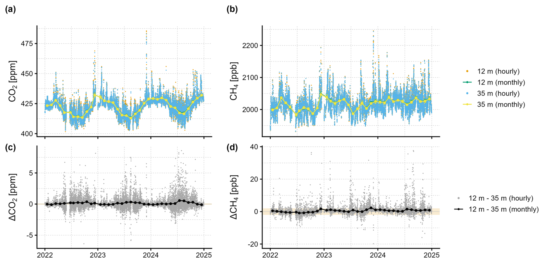
Figure 4 Time series of hourly and monthly mean CO₂ and CH₄ mole fractions measured at Schauinsland station at an intake height of 12 m (orange and green) and 35 m (blue and yellow) in panel (a) and (b). Panel (c) and (d) show the hourly (gray) and monthly mean mole fraction difference (black) between the two routine lines (12–35 m). The WMO/GAW network compatibility goal of 0.1 ppm on CO₂ and 2 ppb on CH₄ mole fractions is indicated in beige.

3 Results and discussion

3.1 CO₂ and CH₄ measurements at 12 and 35 m intake height

Since October 2021, CO₂ and CH₄ mole fractions have been measured simultaneously at the routine intake height of 12 m and at the radio tower at 35 m at Schauinsland station. The comparison of the two intake heights is based on three full years of in situ data, from 2022 to 2024 (Fig. 4a and b). The hourly mean CO₂ mole fractions reach from 401.7 to 485.5 ppm at 12 m and from 402.6 to 482.7 ppm at 35 m, while the hourly mean CH₄ mole fractions reach from 1930.9 to 2245.4 ppb at 12 m and from 1931.9 to 2243.4 ppb at 35 m. The hourly difference in CO₂ and CH₄ mole fraction between the two intake lines (12–35 m) is shown in Fig. 4c and d. Summer measurements show large variability in mole fraction differences between the two intake lines compared to winter, with a signal that fluctuates in both positive and negative directions, reaching from −6.4 to +8.6 ppm in CO₂ and up to 37.6 ppb in CH₄. Monthly mean differences are up to 0.56 ppm in CO₂ and up to 2.3 ppb in CH₄ (Fig. 4).

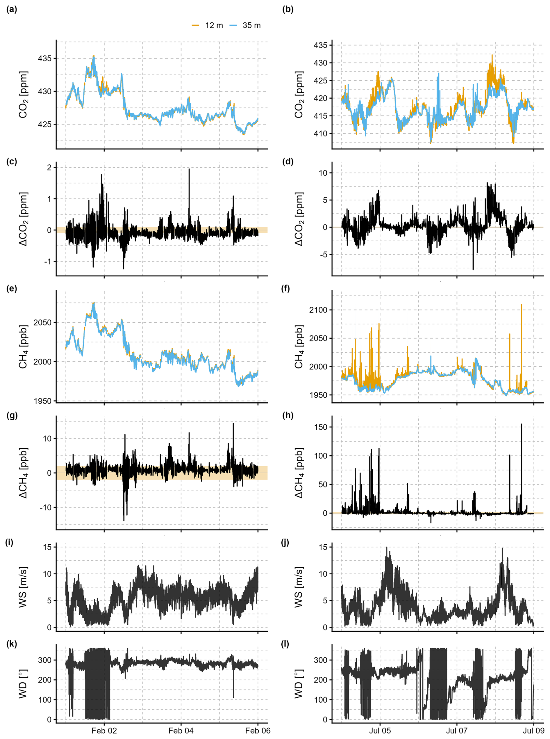
Figure 5 Time series of minutely CO₂ and CH₄ mole fractions measured at Schauinsland station from 1 to 5 February 2024 (left) and from 4 to 8 July 2023 (right). The CO₂ mole fraction is depicted in panel (a) and (b) and the CH₄ mole fraction in panel (e) and (f) (12 m intake line in orange, 35 m in blue). Minutely mean CO₂ mole fraction differences (12–35 m) are shown in panel (c) and (d), and CH₄ mole fraction differences in panel (g) and (h), with the WMO/GAW compatibility goal in beige. Panel (i) to (l) depict the minutely wind speed (WS) and wind direction (WD).

Figure 5 shows two typical five-day time series of atmospheric CO₂ and CH₄ mole fractions at Schauinsland for a winter period (1–5 February 2024) and a summer period (4–8 July 2023). In winter, the main wind direction is west-southwest with an average wind speed of 5.0 ± 3.0 m s⁻¹. In the example period, the minutely CO₂ mole fraction is ranging from 423.40 to 435.44 ppm at 12 m and from 423.60 to 435.22 ppm at 35 m (Fig. 5a). The minutely CH₄ mole fraction is reaching from 1970.2 to 2075.7 ppb at 12 m and from 1968.5 to 2074.9 ppb at 35 m (Fig. 5e). Overall, the measurements at the two intake heights agree well with a mean difference (12–35 m) of $-\mathrm{0.08}\pm$ 0.18 ppm in CO₂ and $+\mathrm{1.0}\pm$ 1.3 ppb in CH₄ averaged over the five-day period (Fig. 5c and g). However, on certain days, elevated CO₂ mole fractions are observed at the 12 m intake, occasionally reaching CO₂ enhancements of up to 2 ppm compared to the 35 m intake, most notably during the night of 1 to 2 February 2024 and again on 4 February 2024. Such enhancements, which are monitored at the 12 m but not at the 35 m intake, are presumably related to local CO₂ fluxes that are more important at the lower intake height. During winter, nocturnal soil fluxes may lead to an accumulation of CO₂ near the surface, thereby affecting the 12 m intake while leaving the 35 m intake largely unaffected. Winter days usually do not show a regular diurnal cycle, both in CO₂ and CH₄, as the biosphere activity is low and the station is above the inversion layer of the Rhine valley for several consecutive days. Larger peaks are usually associated with large-scale transport patterns or a dissolving inversion layer transporting air masses enriched with CO₂ and CH₄ to the station. When these air masses reach the station, they cause elevated mole fractions in both trace gases. For example, an enhancement of nearly 10 ppm in CO₂ and 80 ppb in CH₄ was observed on 1 and 2 February 2024. After 2 February 2024, the baseline in CO₂ and CH₄ is several parts per million or several dozen parts per billion lower than before.

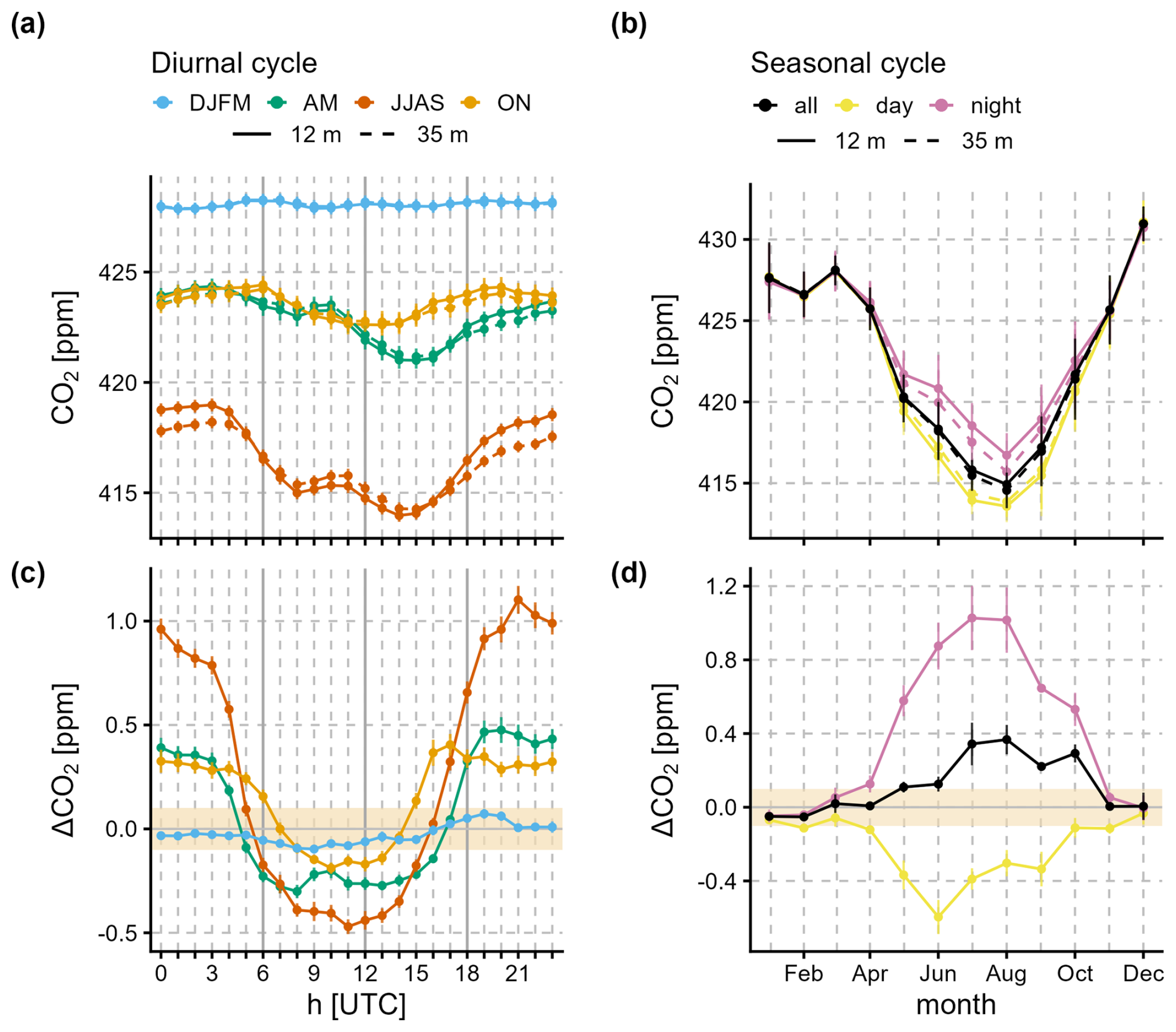
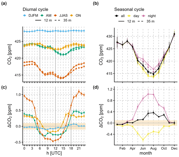
Figure 6 Diurnal mean CO₂ mole fractions grouped by months DJFM (December, January, February, and March, blue line), AM (April and May, green line), JJAS (June, July, August and, September, red line), and ON (October and November, orange line) in panel (a). Panel (b) shows seasonal mean mole fractions for all hours of the day (black) as well as daytime (07:00–15:00 UTC, yellow line) and night-time (21:00–05:00 UTC, purple line). The CO₂ mole fraction at 12 m intake height corresponds to the solid line and at 35 m intake height to the dashed line. The mole fraction difference (12–35 m) is shown in panel (c) and (d), where the beige area marks the WMO/GAW compatibility goal of 0.1 ppm. The error bars represent the standard error of the seasonal mean. The data are based on measurements from 2022 to 2024.

In summer, wind speed is with 3.3± 1.9 m s⁻¹ on average lower compared to winter and again the main wind direction at the station is west-southwest. The period from 4 to 8 July 2023 illustrates a typical summer record for CO₂ and CH₄ at Schauinsland station. The minutely CO₂ mole fraction shows larger variations at 12 m than at 35 m, ranging from 404.77 to 432.27 ppm at 12 m compared to 407.55 to 427.08 ppm at 35 m. Also the minutely CH₄ mole fraction covers a larger range at 12 m, from 1948.4 to 2109.2 ppb, versus 1949.0 to 2018.8 ppb at 35 m. The mean difference between the two intake heights is $+\mathrm{0.27}\pm$ 1.55 ppm for CO₂ and $+\mathrm{1.3}\pm$ 6.7 ppb for CH₄ (Fig. 5d and h).

A distinct diurnal cycle in the CO₂ mole fraction is visible due to biospheric processes. Photosynthesis reduces CO₂ during the day, while respiration increases it at night. The diurnal CO₂ cycle has a stronger amplitude for the 12 m intake, which is closer to the surrounding vegetation than the 35 m intake.

The diurnal CH₄ cycle is much less pronounced in summer than for CO₂ and mostly driven by the dynamics of the PBL. Around noon, air masses from the upper Rhine valley reach the station causing a peak in CH₄, which also can be seen in the CO₂ mole fraction. The origin of these air masses was examined in detail in Schmidt et al. (1996) and is linked to upslope winds and the increase of the PBL height. During periods when these relatively polluted air masses are sampled, the complex transport from areas of high anthropogenic CO₂ and CH₄ emission in the Rhine valley to the station combined with potential CO₂ uptake by the surrounding forest along the transport pathway can generate large fluctuations in the measured CO₂ mole fraction and the mole fraction difference between the two lines.

Furthermore, the minutely CH₄ mole fraction at 12 m shows sharp spikes of up to 100 ppb, as observed on 4 and 5 July 2023. Such events occur regularly during the summer months. Depending on the number of spike events and their height, even hourly data show significantly increased CH₄ values. These local enhancements are attributed to cows grazing at the surrounding pastures, some of which are only a few dozen meters from the station, as described in detail in Hoheisel (2021), and are analyzed further in Sect. 3.4 and 3.5.

3.2 Differences between the intake heights in mean diurnal and seasonal CO₂ cycles

Figure 6 presents the mean diurnal cycle for CO₂ mole fraction during the four seasons (Fig. 6a) and the mean seasonal CO₂ cycles for daytime and night-time (Fig. 6b). Measurements at 12 m intake height are shown as solid lines and the 35 m height as dashed lines. The corresponding differences between the two intake heights (12–35 m) are shown in the lower panels (Fig. 6c and d).

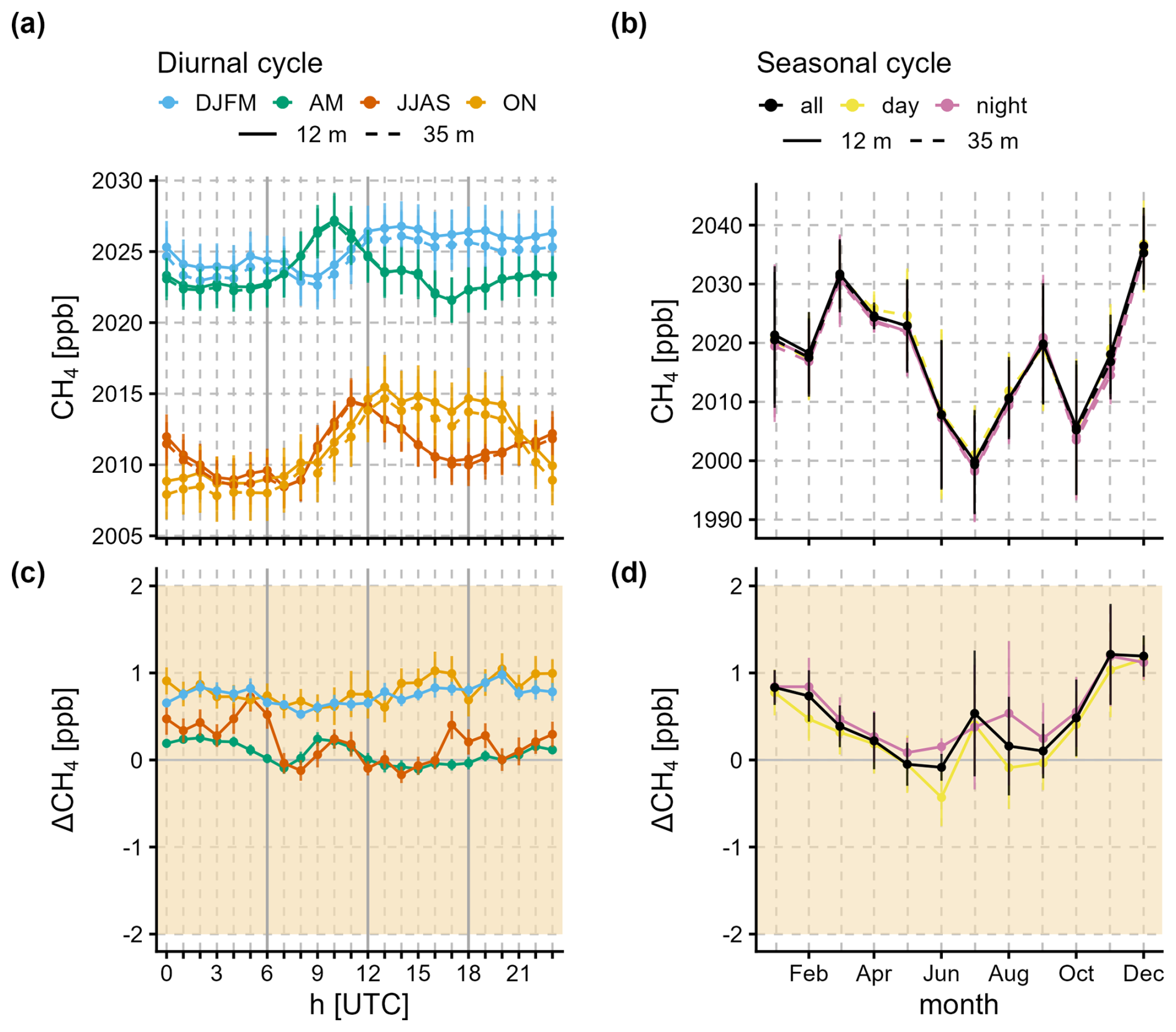
Figure 7 The diurnal mean CH₄ mole fractions grouped by months DJFM (December, January, February, and March, blue line), AM (April and May, green line), JJAS (June, July, August and, September, red line), and ON (October and November, orange line) in panel (a). Panel (b) shows seasonal mean CH₄ mole fractions considering all hours of the day (black), daytime (07:00–15:00 UTC, yellow line) and night-time (21:00–05:00 UTC, purple line). The CH₄ mole fraction at 12 m intake height is shown as solid line and at 35 m intake height as dashed line. The mole fraction difference (12–35 m) is shown in the panel (c) and (d), where the beige area marks the WMO/GAW compatibility goal of 2 ppb. The error bars represent the standard error of the seasonal mean. The data are based on measurements during the years 2022 to 2024.

In winter (DJFM), the mean diurnal CO₂ cycles (Fig. 5a) exhibit only weak peak-to-peak amplitudes of ∼ 0.40 ppm at both intake heights. In contrast, during the summer months (JJAS), the mean CO₂ diurnal cycle shows a much more pronounced pattern, with peak-to-peak amplitudes of 5.0 ± 0.4 ppm at 12 m (red solid line) and 3.9 ± 0.4 ppm at 35 m (red dashed line). The CO₂ mole fractions are lower during the daytime and higher at night, which is due to the respiration and photosynthesis of the biosphere in the surrounding of Schauinsland station. Furthermore, we notice the previously mentioned peak from 09:00–11:00 UTC (11:00–13:00 CEST) attributed to emissions from the Rhine valley (Schmidt et al., 2003). In spring and summer, this process is visible as an enhancement of several parts per million superimposed onto the natural diurnal signal.

The diurnal mean CO₂ difference between 12 and 35 m is illustrated in Fig. 6c. In summer (red line) the CO₂ difference shows a clear diurnal pattern: From 06:00–16:00 UTC the difference is negative, indicating higher CO₂ mole fractions at 35 m, with a minimum of −0.5 ppm around noon. At night (17:00–04:00 UTC), the mean mole fraction difference is positive reaching up to 1.1 ppm at midnight. This periodic pattern in summer is to be explained by the influence of the local biosphere, which has a larger impact on the lower intake line at 12 m than on the higher intake line at 35 m. During the winter months (blue lines) there is no significant difference between the two intake heights, the CO₂ mole fraction difference remains below ± 0.1 ppm throughout the day. In spring and autumn, the diurnal mean CO₂ mole fraction differences between the two intake heights range from −0.3 to +0.5 ppm and from −0.2 to +0.4 ppm respectively.

The mean seasonal cycle in CO₂, calculated from the monthly mean values, shows a clear pattern, with higher mole fractions in early spring and lower in late summer and similar amplitudes at the 12 and 35 m intake height (Fig.  6b). The peak-to-peak amplitude of the seasonal cycle is 1 to 2 ppm larger when considering only daytime data (07:00–15:00 UTC, yellow line) and about 2 ppm smaller, when only considering night-time data (21:00–05:00 UTC, purple line). Due to a pronounced diurnal cycle, the largest differences between daytime and night-time seasonal mean CO₂ mole fractions occur from June to September, with enhanced or reduced amplitudes when considering only daytime or night-time data, respectively.

A seasonal pattern is also visible in Fig. 6d, presenting the monthly mean CO₂ mole fraction difference between the 12 and the 35 m intake line (12–35 m). Differences are most pronounced in summer (June to September) with 0.26 ± 0.15 ppm on average and the largest value reaching +0.37 ppm in August. Similar to the diurnal cycles, the seasonal mean mole fractions show positive differences, or higher mole fractions at 12 m, during night-time, that reach up to +1.0 ppm in July and August (purple line). In contrast, negative differences, or lower mole fractions at 12 m, are observed during daytime with a minimum of −0.60 ppm in June (yellow line). The non-negligible differences between the intake heights from April to October are to be explained by the largely active biosphere, as previously mentioned. Measurements of the CO₂ soil emission rate at Schauinsland station by Hoheisel (2021) also confirm the annual cycle with 7 gCO₂ d⁻¹ m⁻² in July 2020 and 4 gCO₂ d⁻¹ m⁻² in October 2020.

3.3 Differences between the intake heights in mean diurnal and seasonal CH₄ cycles

The mean diurnal variation in CH₄ mole fractions is relatively weak with similar peak-to-peak amplitudes at 12 and 35 m (Fig. 7a). A slight daytime increase with a peak due to upslope wind from the Rhine valley is observed in spring, summer, and autumn. The CH₄ mole fraction differences between the two intake heights are smaller than ± 1 ppb almost the entire day in all seasons and show no significant diurnal variation (Fig. 7c).

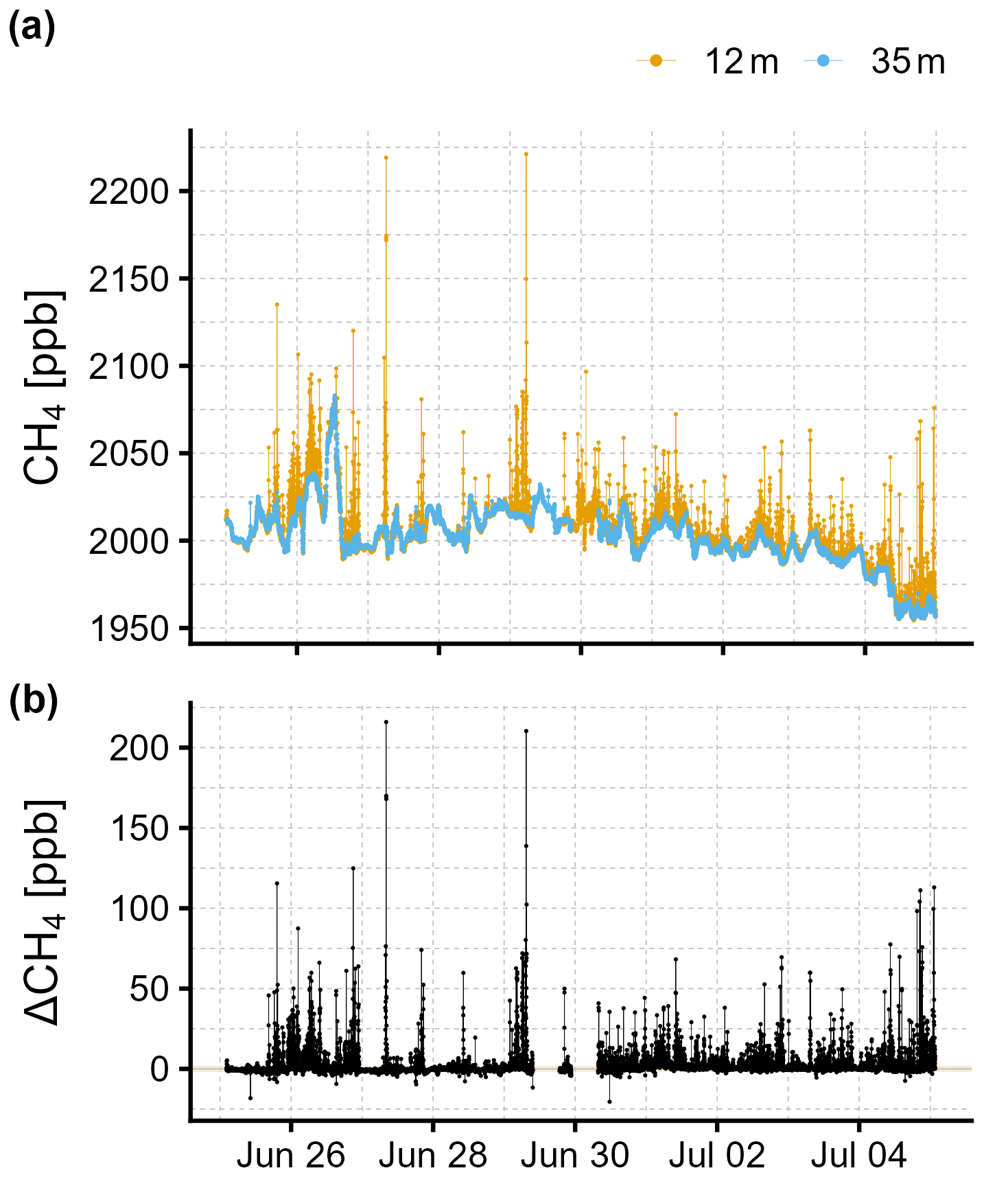
Figure 8 Minutely CH₄ mole fraction measured at 12 m (orange) and 35 m intake height (blue) at Schauinsland station from 25 June 2023 to 4 July 2023 in panel (a) and the corresponding differences (12–35 m) in panel (b). The 12 m time series shows frequent spikes, which are attributed to local pollution. The WMO/GAW compatibility goal of 2 ppb is indicated in beige.

The mean seasonal CH₄ cycle (Fig. 7b) shows maximal mole fractions in March and minimal in July and October with similar amplitudes at both intake heights. The seasonality with increased mole fractions in winter and decreased mole fractions in summer reflects the seasonally changing solar irradiation driving the atmospheric CH₄ sink. Superimposed on this seasonality are patterns related to regional transport: From April to November, CH₄ enriched air masses are transported to the station more frequently leading to elevated mole fractions, especially in August and September. The mean seasonal cycles based on daytime (07:00–15:00 UTC, yellow line) or night-time data (21:00–05:00 UTC, purple line) show very little difference to the seasonal cycle including all hours of the day (Fig. 7b). In contrast to CO₂, the difference in seasonal mean CH₄ mole fraction between the two intake heights is negligible with less than ± 1.2 ppb (Fig. 7d). Nevertheless, we notice relatively low mole fractions at 12 m with respect to 35 m during summer, presumably linked to the CH₄ soil sink in the vicinity of the station, which is more important at the lower intake height and predominantly active from May to September: Hoheisel (2021) determined the CH₄ soil uptake at Schauinsland station with flux chamber measurements to approximately −0.6 mg CH₄ d⁻¹ m⁻² in July 2020 and to −0.08 mg CH₄ d⁻¹ m⁻² in October 2020.

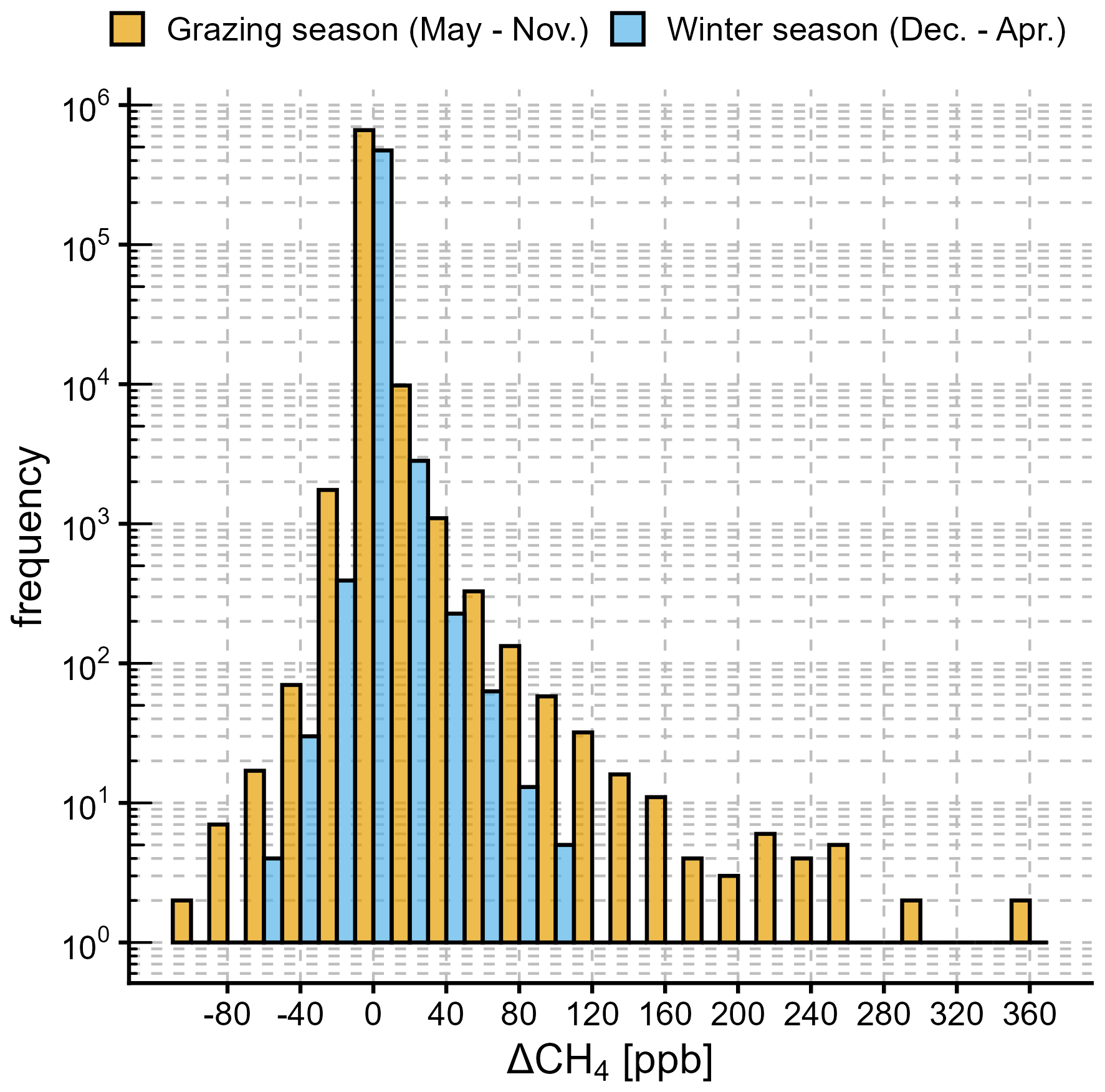
Figure 9 Distribution of minutely CH₄ mole fraction differences ($n=\mathrm{1.15}\times {\mathrm{10}}^{\mathrm{6}}$) between the two intake heights (12–35 m) during grazing season (May to November) in orange and during winter season (December to April) in blue.

3.4 Comparison of CH₄ spikes at 12 and 35 m

At Schauinsland station, spikes in the 12 m CH₄ time series are observed frequently during summer and autumn months (May to November) and are attributed to cows grazing on the meadows around the station, some located only a few dozen meters from the air intake system. The spikes occur irregularly throughout the grazing season and are clustered over periods ranging from several days up to few weeks with enhancements up to 369 ppb in minutely and 38 ppb in hourly CH₄ values.

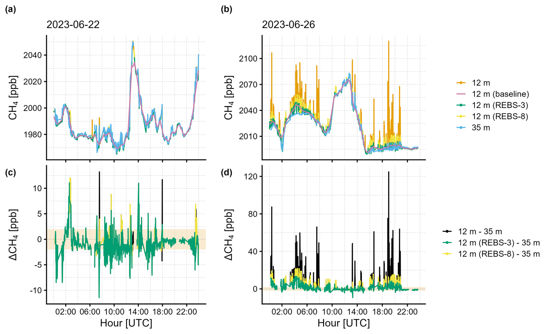
Figure 10 Minutely CH₄ mole fraction at 12 m without filtering (orange), after applying the REBS algorithm with β=3 and 8 (green and yellow, respectively), and at 35 m (blue) measured on 22 June 2023 in panel (a) and on 26 June 2023 in panel (b). The baseline calculated by the REBS algorithm is shown in purple. In panel (c) and (d), the mole fraction difference between the sampling heights (12–35 m) without filtering is shown in black and after applying the REBS algorithm with β=3 and 8 in green and yellow, respectively. The WMO/GAW compatibility goal of 2 ppb is marked in beige.

These local pollution events are at the same order of magnitude as CH₄ spikes due to a local sewage treatment facility at Pic du Midi station, France (El Yazidi et al., 2018) or as CH₄ spikes at the coastal station Westerland, Germany related to marine sand dredging activities (Schmidt et al., 2026a). However, they are relatively small compared to the Ispra station, Italy, where livestock-related CH₄ spikes of up to few parts per million were reported (Cristofanelli et al., 2023).

CH₄ mole fractions measured at 12 and 35 m from 25 June to 5 July 2023 are exemplarily shown in Fig. 8a. During this time, frequent spikes with an enhancement of up to 216 ppb in minutely CH₄ values are observed at the 12 m intake height. Averaged over the full 10 d period, the CH₄ mole fraction at 12 m is enhanced by 2.7 ± 9.0 ppb compared to the 35 m intake height (Fig. 8b). As shown in the example and confirmed by the full three years of parallel measurements, the CH₄ time series at 35 m is largely unaffected by local spikes indicating that this height is not influenced by nearby cattle emissions.

Figure 9 shows a histogram of the minutely CH₄ mole fraction difference between the two intake heights over the three-year period. During the grazing season (May to November), when cows may be present near the station, the distribution (orange bars) is broader with 0.31 ± 4.18 ppb compared to winter season with 0.62 ± 2.12 ppb (blue bars). Mole fraction differences between the two intake heights larger than 20 ppb are observed 3 to 14 times more often during grazing season.

Table 2 Percentage of the hourly values after filtering with the REBS algorithm that show a difference to the original data set within a certain interval.

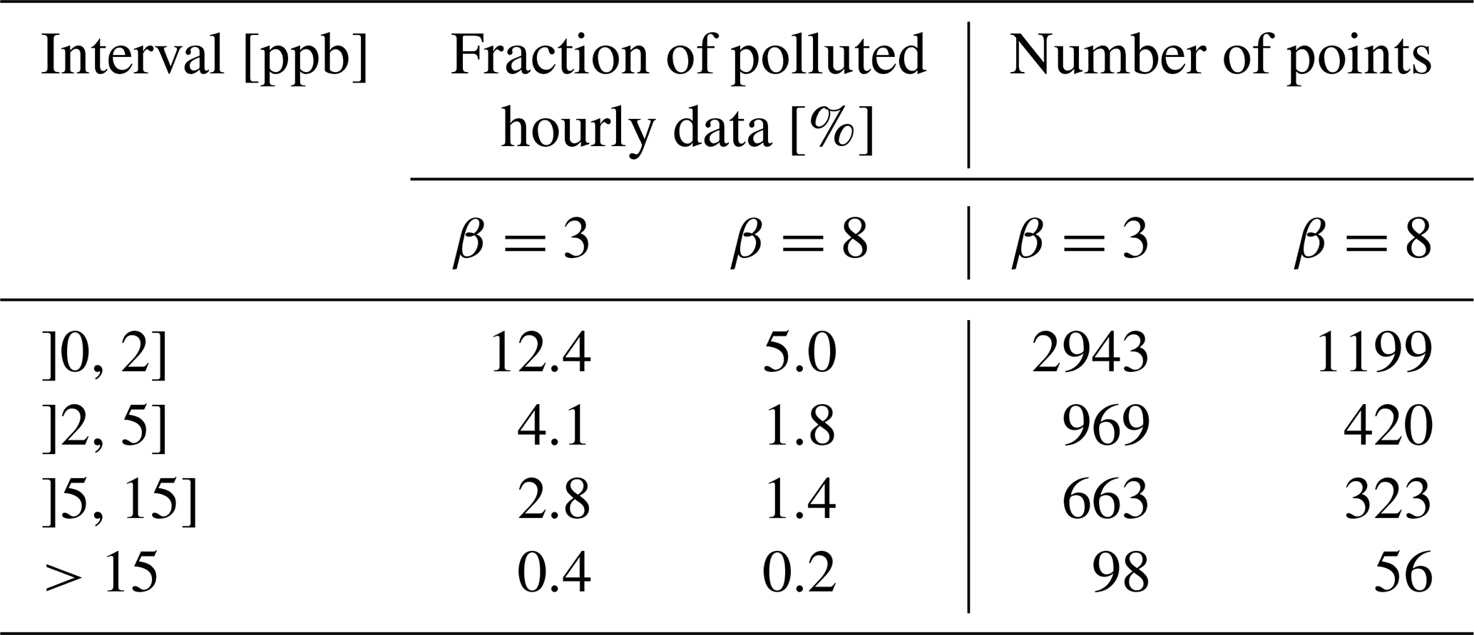
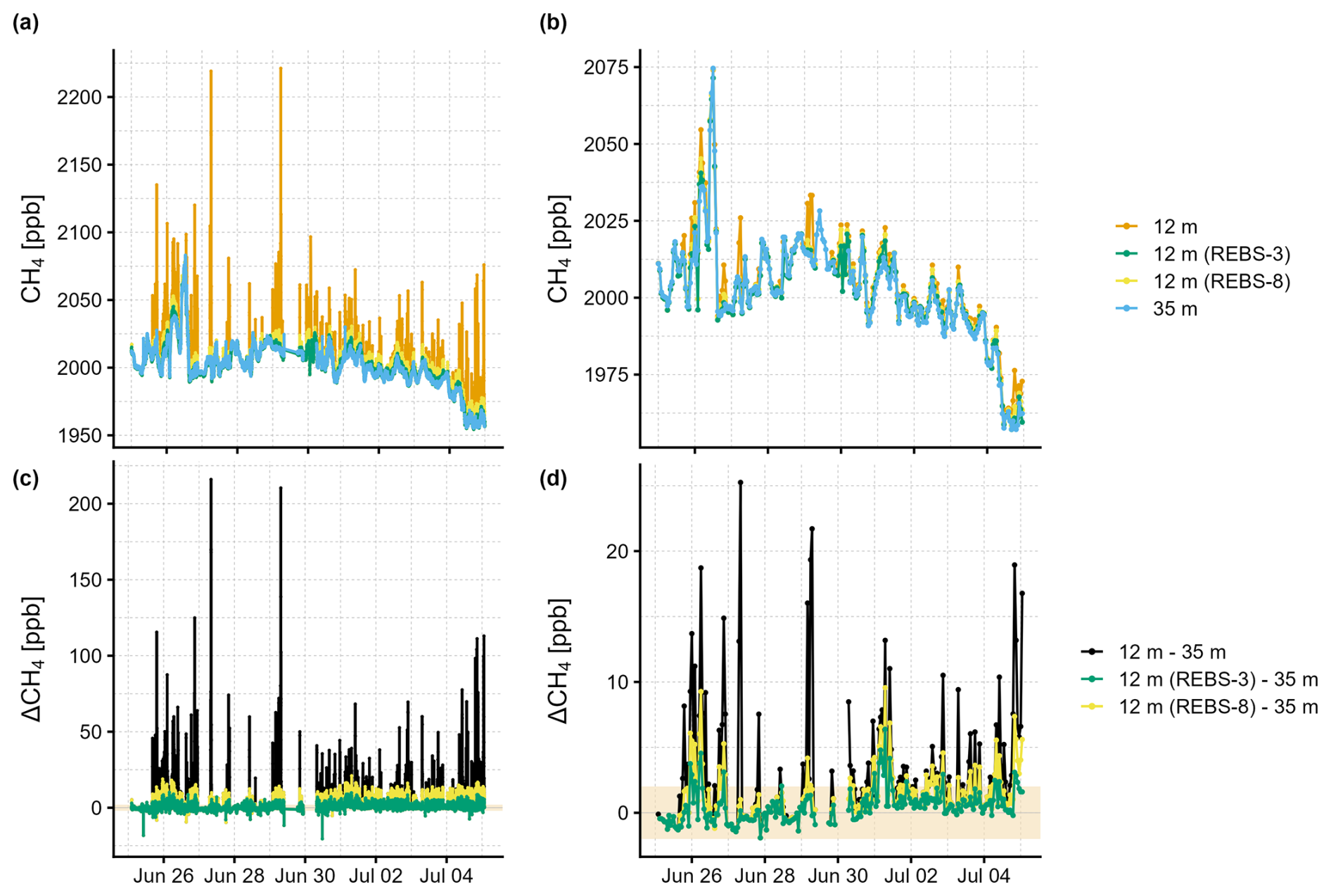
Figure 11 Example time series of minutely mean CH₄ mole fractions at 12 m (orange) and 35 m (blue) from 25 June to 5 July 2023 in panel (a). The minutely mean CH₄ mole fraction at 12 m after application of the REBS algorithm with β=3 and β=8 is shown in green and yellow, respectively. Panel (c) shows the minutely mole fraction differences (12–35 m) without filtering in black and after applying the algorithm in green and yellow. The minutely CH₄ mole fractions and the differences are averaged over hours and shown in panel (b) and (d). The WMO/GAW compatibility goal of 2 ppb is indicated with in beige in the lower two panels.

3.5 Performance of automatic CH₄ spike detection at 12 m

To quantify the influence of local CH₄ spikes on the 12 m time series and to assess potential biases in the historic record, we need an effective method to detect the highly frequent CH₄ spikes. Spike detection in the ICOS atmospheric network commonly relies on manual flagging by the station manager or an automatic algorithm using the standard deviation of the background (SD), as described and tested in studies by El Yazidi et al. (2018) and Cristofanelli et al. (2023). At Schauinsland station, the highly frequent CH₄ spikes render manual flagging impractical and introduce subjectivity. We therefore tested and compared several automatic spike-detection algorithms to identify a suitable approach for this site.

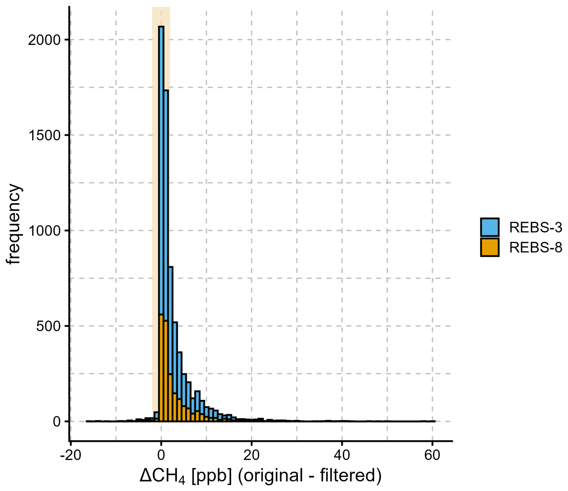
Figure 12 Histogram of the difference between the original hourly mean CH₄ mole fractions and the hourly mean CH₄ mole fractions after applying the REBS spike detection algorithm with β=3 (blue, n=4831) and β=8 (orange, n=2056). Hourly mean mole fractions that remain untouched by the filtering are not counted in the histogram. The WMO/GAW compatibility goal of 2 ppb is shown in beige.

Cristofanelli et al. (2023) evaluated multiple spike detection algorithms at various ICOS stations (excluding Schauinsland station) and concluded that each station may require a tailored algorithm depending on local conditions and spike behaviour. Based on these findings and considering performance and robustness, we tested two algorithms for spike detection. First, the SD algorithm, which identifies spikes based on deviations from the background signal expressed by the standard deviation (Drewnick et al., 2012). Under various configurations, this method was found to retain too much data during periods of very frequent spiking and was therefore not suitable for the CH₄ spikes at Schauinsland station (Fig. S3). Second, we selected an automatic method using the Robust Extraction of Baseline Signal (REBS) spike detection algorithm (Ruckstuhl et al., 2012) to detect spikes in the 12 m CH₄ time series (Eq. 1).

The REBS algorithm effectively detects spikes while maintaining a low false detection rate for highly variable data, which makes it particularly well suited for time series dominated by frequent spikes originating from local sources (Cristofanelli et al., 2023). The choice of the REBS parameter β is a trade-off between correctly detecting spikes associated to local pollution and avoiding misclassification of short-scale signal from turbulence fluctuations. In sensitivity tests performed in this study, the parameter β was varied between 1 and 10 (Figs. S4, S5, and S6). The bandwidth also influences the performance of the algorithm and was set to 60 min consistent with previous applications by El Yazidi et al. (2018) and Cristofanelli et al. (2023). A qualitative sensitivity test can be found in the Supplement (Fig. S7).

To investigate the behavior of the algorithm in detail, a case study on two days with and without spikes is conducted and shown in Fig. 10 for the default configuration β=3 as well as β=8. On 22 June 2023, no spikes attributed to cow emissions were observed at the station (Fig. 10a and c). Nevertheless, the algorithm identifies 126 for β=3, whereas 26 were detected for β=8. In contrast, during the spike intense day of 26 June 2023, the more stringent configuration with β=3 is able to identify a much large number of spikes (272), while for β=8 only 118 spikes are identified (Fig. 10b and d). Unfortunately, even configurations with low β values are less sensitive during spike intense periods, as the baseline (purple line) is overestimated by the algorithm (Ruckstuhl et al., 2001; El Yazidi et al., 2018). Since the 35 m intake height is largely unaffected by local spikes, the difference between the filtered 12 and the 35 m time series can be used to evaluate the performance of the spike detection. During the example period, spikes in the CH₄ mole fraction up to 22 ppb for β=8 and up to 14 ppb for β=3 remain after filtering. Overall, the REBS algorithm performs well during periods with moderate spikes, especially for β=3, and found suitable to detect the very frequent spikes originating from a local source. However, as this configuration tends to overestimate the spikes under low-spike condition, it is not recommended without manual control.

3.6 Impact of the automatic CH₄ spike detection on the 12 m time series

The REBS spike detection algorithm was applied to the minutely CH₄ mole fraction at 12 m using two configurations, β=3 and β=8 (Fig. 11a). Based on the a priori knowledge that cows may be grazing at the meadows around the station from May to November, and supported by an analysis of high-frequency CH₄ data, the algorithm is applied exclusively to data from the defined grazing season. Relative to the estimated baseline of CH₄ mole fraction, the data are classified as spike or background mole fraction by the algorithm. The time series after filtering is shown in Fig. 11a in green and yellow for β=3 and β=8, respectively. Figure 11b shows the respective CH₄ mole fractions averaged to hourly mean values and Fig. 11c and d show the mole fraction differences between the intake heights.

During this 10 d test period, 16.0 % (6.1 %) of the minutely data are flagged as spike by the REBS algorithm with β=3 (β=8), which decreases the minutely CH₄ mole fraction at 12 m up to 219.7 ppb (218.7 ppb) and by 2.7 ppb (1.7 ppb) on average compared to the original data set. The corresponding hourly mean CH₄ mole fraction at 12 m is reduced up to 27.3 ppb (26.1 ppb). The performance of the spike-detection algorithm can be assessed by comparing the filtered 12 m time series with the measurements at 35 m (Fig. 11c and d). As noted previously, periods characterized by very frequent spiking, e.g. on 25 and 26 June 2023, remain challenging for the algorithm. During these intervals, the CH₄ mole fraction difference between the REBS-filtered 12 m data and the 35 m time series remains high with up to 9.8 ppb (21 ppb) in minutely and up to 6.4 ppb (9.6 ppb) in hourly data.

Finally, the REBS algorithm with β=3 (β=8) is applied to the minutely CH₄ mole fraction during grazing season (May to November) from 2022 to 2024, identifying 7.9 % (2.3 %) of the minutely data during the grazing period and 4.6 % (1.3 %) of the entire minutely data set as spike. In order to quantify the influence of the REBS algorithm on the 12 m time series, the difference between hourly mean mole fractions after filtering with the REBS algorithm and the original data set is evaluated (Fig. 12 and Table 2).

From 2022 to 2024, 20.3 % (8.6 %) of the hourly values are affected by the filtering with the REBS algorithm with β=3 (β=8). 7.3 % (3.4 %) of the hourly mean mole fractions deviate to the original values after filtering with β=3 (β=8) by more than 2 ppb, 4.1 % (1.8 %) of the data fall within an intermediate range of 2 to 5 ppb, and 2.8 % (1.4 %) or 0.4 % (0.2 %) in a larger range of 5 to 15 ppb and more than 15 ppb respectively. Monthly mean CH₄ mole fractions deviate to the original time series after application of the filtering by up to 1.8 and 0.8 ppb for β=3 and β=8, respectively (Fig. S9).

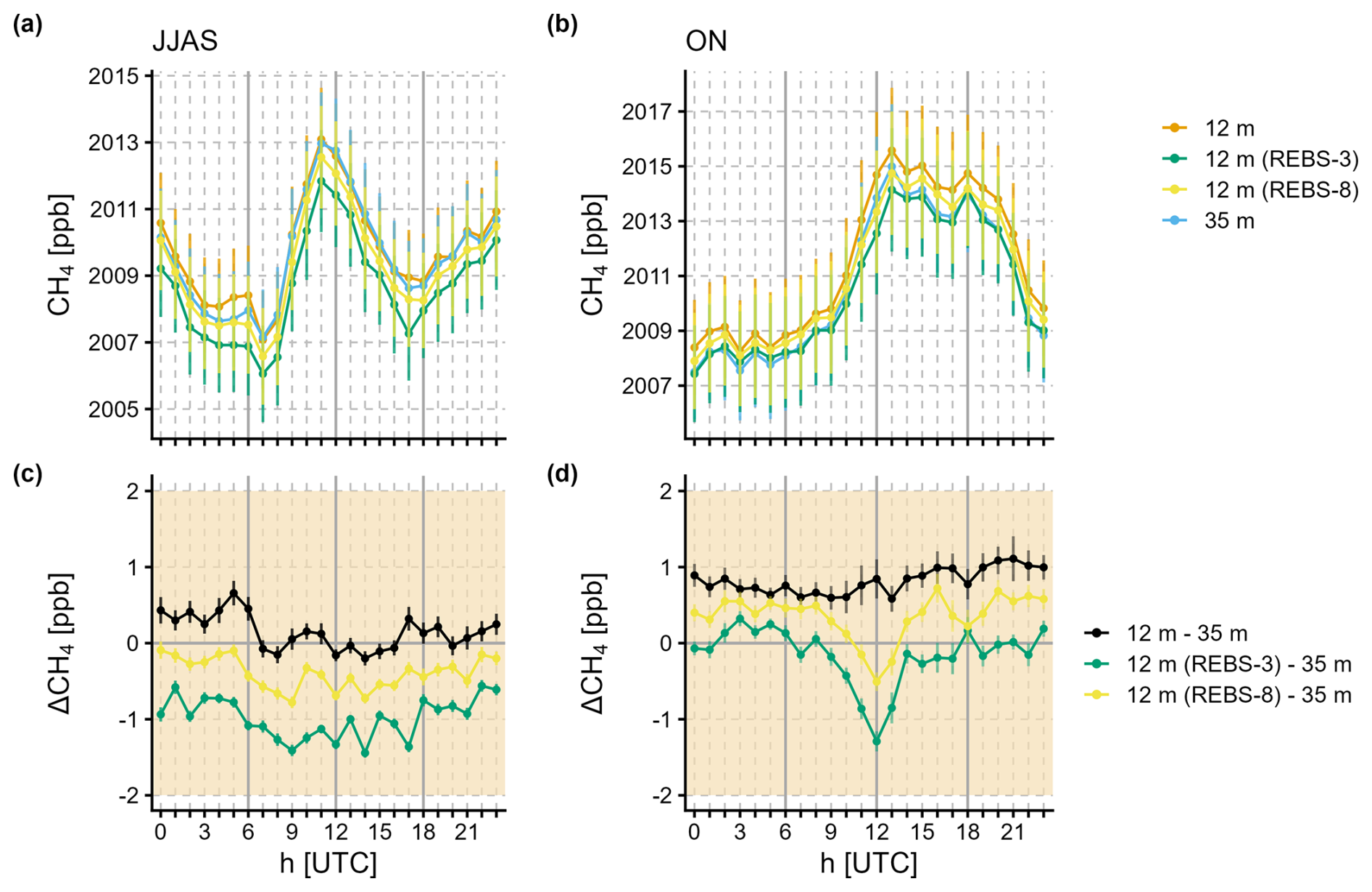
Figure 13 Diurnal mean CH₄ mole fractions during summer (June, July, August, September) and autumn (October and November). The plots (a) and (b) show the mole fraction at 12 m without application of the REBS algorithm (orange), after filtering with the REBS algorithm with β=3 (green), after filtering with β=8 (yellow) and at 35 m (blue). The mole fraction difference between the corresponding time series are shown in panel (c) and (d). The error bars represent the standard error of the seasonal mean. The WMO/GAW compatibility goal of 2 ppb is indicated in beige.

Figure 13 shows the diurnal mean CH₄ mole fractions and the differences between the 12 and 35 m intake estimated for the original and the filtered data set, analogously to Sect. 3.3. The diurnal mean mole fraction in summer (June, July, August, September) is up to 1.7 ppb (0.9 ppb) and in autumn (October and November) up to 2.1 ppb (1.4 ppb) lower after application of the REBS algorithm with β=3 (β=8). The filtered time series shows deviations to the original time series >2 pbb for β=3 in autumn around noon time, when the planetary boundary layer height exceeds the height of the station and air from the Rhine valley reaches the station. During this time the CH₄ mole fractions show large variations and the REBS algorithm with β=3 is overestimating the spikes leading to biases.

Finally, the distribution of hourly values that are affected by the spike detection over the day indicates that the spikes tend to occur more often during daytime (05:00–19:00 UTC) than during night-time and in the month of July, related to the grazing behavior and movement of the cows (Fig. S10). Moreover, most spikes are originating from west-southwest since this is the main wind direction and the largest meadows are also located in this sector (Fig. S11). However, meadows are located all around the station and a non-negligible part of the spikes also occurs in the north and south-east sector. This makes it very difficult to develop adequate selection criteria based on the wind direction. Similarly, a wind speed filter cannot be applied as the spikes occur at low and high wind speeds, stressing the need for the demonstrated filtering method.

4 Conclusions

In this study, three years of continuous CO₂ and CH₄ CRDS measurements at Schauinsland station, Germany have been evaluated to quantify the impact of measurement height on the respective time series. While measurements at Schauinsland station have historically been conducted at 6 m a.g.l. and since 2005 at 12 m a.g.l., an additional air intake system at 35 m was installed on a nearby radio tower in September 2021. Since then, both heights have been operated in parallel enabling a detailed comparison of diurnal and seasonal differences as well as the influence of local CH₄ pollution events.

The comparison revealed systematic differences between the two inlet heights, particularly during summer. During daytime, the mean diurnal CO₂ mole fraction are up to 0.5 ppm higher at 35 m, whereas night-time values are up to 1.1 ppm higher at 12 m. Accordingly, the monthly mean CO₂ mole fraction in summer is on average 0.26 ± 0.15 ppm higher at 12 m than at 35 m, reaching a difference up to 0.56 ppm. These findings indicate a larger influence of local biospheric fluxes on the 12 m record during summer, while the 35 m inlet is less affected by local variability. In winter (November–February), both diurnal and monthly mean differences are small (within ± 0.1 ppm). With the installation of the measurement equipment into a new building approximately 40 m northeast of the current station in summer 2025, the results of this study provide a valuable reference for evaluating the continuity of the Schauinsland CO₂ time series. The 35 m record can serve as a stable reference to bridge potential discontinuities in the 12 m series caused by the relocation. Furthermore, the detected vertical CO₂ gradients suggest that local biospheric fluxes may have influenced the long-term 12 m record to a non-negligible degree, especially under changing vegetation and climate conditions in recent decades (Ramonet et al., 2020; Van der Woude et al., 2023). Complementary low frequency eddy covariance measurements using the 35 m sampling inlet could give further insights into the local biosphere at low effort (Herig Coimbra et al., 2024).

The CH₄ mole fraction differences between the two intake heights are smaller than ± 1 ppb in diurnal and seasonal means. However, local CH₄ pollution events occur regularly between May and November, when cows graze on the meadows around the station from May to November. These events cause CH₄ spikes of up to 369 ppb in minutely and up to 38 ppb in hourly mean mole fractions at 12 m, while the 35 m data remain unaffected. In order to detect and filter the local contamination, a semi-automatic detection method based on the REBS algorithm was tested and applied on the minutely mole fraction at 12 m intake height under a stringent (β=3) and a more conservative configuration (β=8). Over the three-year period, 3.4 % of the hourly mean mole fractions at 12 m after applying the REBS algorithm (β=8) deviate to the original data by more than 2 ppb. Consequently, the observed pollution events could potentially introduce biases in model simulations in the historic CH₄ record measured at 12 m. Therefore, for the CRDS-based CH₄ record, the application of a spike detection algorithm to identify local contamination events in the 12 m measurements should be considered. For earlier measurements with lower temporal resolution, further investigation is required to develop appropriate quality control strategies.

To improve the accuracy of the Schauinsland CH₄ record, the REBS algorithm could be integrated into the ICOS data flagging routine and applied to current and past CRDS data. Due to its tendency toward over-detection, it should preferably be used only from May to November, when cows are present on nearby meadows, and results should be verified by the station PI, especially under the stringent configuration of β=3. The REBS algorithm proved more effective than the SD approach, identifying a larger fraction of invalid data and supporting the findings of Cristofanelli et al. (2023) that spike detection performance is site-specific. Since avoiding spikes is preferable to filtering them out (El Yazidi et al., 2018), future CH₄ analysis should primarily rely on the 35 m sampling line.

Overall, maintaining measurements at both 12 m and 35 m a.g.l. is recommended. For CO₂, continued use of the 12 m inlet ensures consistency with the historical record spanning over five decades, while the 35 m data provide an essential reference for evaluating potential biases. For CH₄, the 35 m time series can reliably extend the historical record without significant loss of continuity. The insights gained here ensure the long-term integrity and comparability of the Schauinsland greenhouse gas observations within the European monitoring network.