Classification-constrained retrieval of PM_2.5 vertical profiles from fluorescence-raman-mie polarization lidar

The vertical distribution of PM_2.5 during urban haze events is jointly affected by aerosol composition, boundary-layer structure, and regional transport. Empirical PM_2.5 retrievals based on lidar-derived extinction coefficients can be biased by the optical contribution of coarse-mode mineral particles. This study used fluorescence–Raman–Mie polarization lidar observations in Beijing to identify anthropogenic pollution aerosols (APA), desert dust (DD), and mineral dust (MD) using the particle depolarization ratio (PDR) and fluorescence capacity (G_f). The classification results were incorporated into the construction and application of an empirical extinction–PM_2.5 relationship. For mixed-aerosol samples, the APA component fraction and its associated extinction contribution were estimated before retrieving the vertical PM_2.5 distribution.

To quantify the effect of classification constraints, three linear models were developed: a model without aerosol-type constraints, a PDR-only screening model, and a model constrained by combined PDR–G_f classification. Near-surface, date-separated validation using 411 hourly samples from 69 observation dates showed that the combined-classification model achieved an RMSE of 17.32 µg m⁻³, an MAE of 13.54 µg m⁻³, and a Bias of 3.30 µg m⁻³. Compared with the model without aerosol-type constraints, the RMSE, MAE, and Bias decreased by 38.2 %, 45.0 %, and approximately 83.0 %, respectively. Uncertainty analysis showed that classification end-member and aerosol-type-dependent lidar-ratio perturbations affected the quantitative PM_2.5 estimates under mixed-aerosol conditions, whereas the residual scatter and parameter stability of the empirical extinction–PM_2.5 relationship were the dominant sources of prediction uncertainty.

For a mixed-to-pollution aerosol evolution episode in Beijing in November 2024, the classification-constrained PM_2.5 vertical structure was physically consistent with temperature stratification, wind fields, and backward trajectories. Seasonal testing showed no stable and consistent improvement from season-specific fitting. The proposed method provides classification-constrained estimates of the PM_2.5 vertical structure under APA-dominated conditions in Beijing. Model parameters should be recalibrated using local observations when applied to regions, seasons, or aerosol conditions with substantially different composition.

1 Introduction

Fine particulate matter (PM_2.5) refers to suspended particles in the atmosphere with an aerodynamic diameter of 2.5 µm or less. It is mainly composed of secondary inorganic aerosols (SIA), including sulfate, nitrate, and ammonium, as well as organic aerosol (OA), elemental carbon (EC), and other components (Zhang et al., 2013). Owing to its small particle size and large specific surface area, PM_2.5 can penetrate deeply into the human respiratory system and induce cardiopulmonary diseases. It is therefore a major pollutant of public-health concern in urban haze pollution (Dockery et al., 1993; Pope III and Dockery, 2006). In recent years, severe pollution episodes have occurred frequently during autumn and winter in urban agglomerations in North China, with Beijing being a representative case. The vertical distribution of PM_2.5 concentration is jointly regulated by boundary-layer thermal conditions, regional transport, and aerosol composition, and the spatiotemporal evolution of its vertical structure is directly associated with pollutant accumulation and dispersion pathways. Therefore, accurately obtaining vertical profiles of PM_2.5 concentration is of great scientific significance for advancing our understanding of pollution-process mechanisms and identifying external transport pathways.

Obtaining vertical profiles of PM_2.5 remains a technical challenge in atmospheric environmental observations. Although ground-based monitoring networks can provide highly accurate near-surface concentration data, they cannot characterize the vertical structure of pollutants. Spaceborne passive remote sensing can retrieve aerosol optical depth (Levy et al., 2013; Hsu et al., 2013) and estimate ground-level PM_2.5 concentrations by combining it with chemical transport models (van Donkelaar et al., 2016) or machine-learning methods (Wei et al., 2020). However, its column-integrated nature likewise prevents the resolution of vertically layered information. Ground-based lidar actively emits laser pulses and receives atmospheric backscattered signals, enabling the acquisition of vertical profiles of aerosol extinction coefficient with high temporal and spatial resolution (Baars et al., 2016; Weitkamp, 2005). It therefore provides an effective approach for retrieving the vertical structure of PM_2.5. Previous studies have established empirical linear models by fitting ground-based PM_2.5 measurements to near-surface lidar-derived extinction coefficients, and have extrapolated these models to the full vertical profile to obtain the vertical distribution of PM_2.5 (Lyu et al., 2018; Tao et al., 2016). This approach has been widely applied in various urban environments, providing important vertical observational support for investigating pollutant transport fluxes (Liu et al., 2019; Tian et al., 2026) and the regulation of pollution accumulation by boundary-layer evolution (Lou et al., 2019).

However, the lidar-based empirical linear models described above implicitly assume that variations in the extinction coefficient are primarily dominated by PM_2.5. In fact, extinction coefficient reflects the integrated effect of all atmospheric aerosol components on optical attenuation. Against the background of anthropogenic pollution with relatively single aerosol composition, the extinction coefficient shows a good linear correlation with PM_2.5. However, under the coexistence of coarse-mode particle pollution and anthropogenic aerosols, which is prevalent in North China during autumn and winter, this relationship becomes systematically biased. The mass extinction efficiency of coarse-mode particles is significantly lower than that of the fine-mode anthropogenic pollution aerosol (APA) class (Ferrare et al., 2025; Tao et al., 2017). If the total extinction coefficient incorporating the contribution of coarse-mode particles is directly substituted into the relationship, the extinction contribution from coarse-mode particles may introduce systematic bias. The extinction-based approaches of Lyu et al. (2018) and Tao et al. (2016) demonstrate the feasibility of deriving vertical PM_2.5 distributions from near-surface extinction–PM_2.5 relationships. However, they do not explicitly separate fine-mode pollution aerosol from coarse-mode mineral aerosol before model fitting. This limits the applicability of empirical models when these components coexist, particularly under varying relative-humidity conditions that further modify aerosol optical properties.

To address the above issues, aerosol classification can be constrained using optical parameters other than the extinction coefficient. The particle depolarization ratio (δ_p), which reflects the degree of particle nonsphericity, is currently a commonly used classification criterion. Spherical APAs are characterized by low depolarization ratios, whereas nonspherical coarse-mode particles, such as dust, exhibit high depolarization ratios (Burton et al., 2012). Based on this parameter, the POLIPHON method (Mamouri and Ansmann, 2014, 2017) has enabled the retrieval of vertical profiles of the mass concentrations of dust and non-dust components by decomposing the total extinction into dust and non-dust contributions and combining them with the mass extinction efficiencies of the respective components. Tian et al. (2026) applied this method in Beijing and successfully distinguished the mass concentration flux structures of dust and anthropogenic aerosols. However, classification schemes relying solely on the depolarization ratio have limitations in mass concentration retrieval. After dust particles undergo internal mixing with anthropogenic pollutants during transport, their morphology tends to become more spherical, leading to a significant decrease in the particle depolarization ratio (Pan et al., 2017; Veselovskii et al., 2022), which causes overlap with the δ_p range of APAs. Meanwhile, relying solely on the depolarization ratio provides no means of further distinguishing the extinction contributions of individual components within the non-dust fraction, thereby limiting its applicability in the accurate retrieval of PM_2.5. The introduction of fluorescence lidar technology has provided a new approach for improving classification accuracy. Fluorescence capacity (G_f) is related to the abundance of fluorescent organic constituents in aerosols (Veselovskii et al., 2020, 2022). PM_2.5 is enriched in organic components, and organic aerosol (OA) can account for 30 %–50 % of its mass during heavy pollution episodes (Huang et al., 2014; Xu et al., 2021). Accordingly, APAs generally exhibit moderate-to-high fluorescence capacity, whereas mineral dust aerosols show weak fluorescence responses (Li et al., 2019; Jiang et al., 2024). Observations in Beijing by Li et al. (2019) confirmed that the correlation between the fluorescence signal and PM_2.5 concentration (r≈0.85) was significantly stronger than that between the extinction coefficient and PM_2.5 concentration (r≈0.69), demonstrating the sensitive response of the fluorescence signal to organic components in PM_2.5. The joint use of G_f and δ_p enables refined aerosol-type discrimination in a two-dimensional parameter space, which cannot be achieved using the depolarization ratio alone. Veselovskii et al. (2022) and Veselovskii et al. (2024) proposed a δ_p–G_f classification framework and a set of equations for the quantitative separation of mixed-aerosol components. Using the same fluorescence–Raman–Mie polarization lidar system in Beijing, Jiang et al. (2024) applied this framework to low-altitude haze aerosols during spring 2024. That study established operational δ_p–G_f ranges for APAs, desert dust (DD), and mineral dust (MD), and used pure-component depolarization and fluorescence parameters to estimate their contributions in mixed-aerosol conditions. However, previous studies based on the δ_p–G_f framework have so far mainly focused on optical-parameter-based component separation, and the potential of these classification results for vertical PM_2.5 mass concentration retrieval remains largely unexplored.

Based on the aerosol classification and component-separation methods described above, this study developed a classification-constrained method for retrieving the vertical structure of PM_2.5 using fluorescence–Raman–Mie polarization lidar observations. The classification results were incorporated into both the construction and application of the empirical extinction–PM_2.5 relationship. During model development, only APA-dominated samples were selected for fitting. During model application, the APA component fraction and its associated extinction contribution were first estimated for mixed-aerosol samples and then used for PM_2.5 retrieval, thereby reducing the interference of coarse-mode particles.

To quantitatively evaluate the effect of classification constraints, three linear models were compared: a model without aerosol-type constraints, a model using PDR-only screening, and a model using combined PDR–G_f classification constraints. The models were evaluated using near-surface matched samples from dates excluded from model training. In addition, the effects of classification end-member parameters, aerosol-type-dependent lidar ratios, extinction-coefficient measurement error, and model parameters on the retrieved PM_2.5 were assessed, together with the applicability of the model under different seasons and aerosol backgrounds. Finally, a mixed-to-pollution aerosol evolution process in Beijing was analyzed using temperature stratification, wind fields, and backward trajectories to examine the physical plausibility of the retrieved PM_2.5 vertical structure.

2 Materials and Methods

2.1 Lidar Systems

The fluorescence–Raman–Mie polarization lidar system used in this study was developed by Zhang et al. (2021) and is located at the Zhongguancun campus of Beijing Institute of Technology (39.96° N, 116.31° E). The system employs a 355 nm Nd:YAG laser as the light source, with a pulse energy of 30 mJ, a repetition frequency of 20 Hz, and a vertical resolution of 7.5 m. The receiving system consists of horizontal/vertical polarization elastic-scattering channels, a 387 nm nitrogen vibrational Raman channel, and a fluorescence-scattering channel, which can be used to retrieve aerosol optical parameters including the extinction coefficient, particle depolarization ratio, and fluorescence capacity. Owing to the influence of the geometrical factor, the minimum valid detection height of the system is 450 m. Detailed system parameters are provided in Zhang et al. (2021). Because the fluorescence channel is sensitive to solar background radiation, the system was operated only at night; therefore, all observational data used in this study were acquired during nighttime.

In this study, a coherent Doppler wind lidar was also used to obtain vertical wind-field profiles, providing wind speed and wind direction information with a vertical resolution of 0.1 km. In addition, a Raman–Mie lidar was employed to retrieve nighttime tropospheric temperature profiles. Both systems were collocated with the fluorescence–Raman lidar at the same observation site, and the resulting datasets were used to analyze the dynamical and thermodynamical background of the pollution transport process.

2.2 Observational Data

Hourly ground-level PM_2.5 mass concentration data were obtained from the Wanliu Station of the Beijing Environmental Protection Monitoring Center (39.96° N, 116.30° E), which is approximately 3 km from the lidar observation site. Humidity data were derived from radiosonde observations at the Beijing 54511 meteorological station (39.81° N, 116.47° E), located approximately 20 km from the lidar observation site. All times reported in this study are in Coordinated Universal Time (UTC).

2.3 Methods

2.3.1 Data Processing Methods

The aerosol extinction coefficient α was retrieved from the 387 nm nitrogen vibrational Raman-channel signal using the Raman method (Ansmann et al., 1990). This method does not require an assumed lidar ratio (LR) and can directly provide extinction coefficient profiles at 355 nm. The particle depolarization ratio (PDR, δ_p), which characterizes the degree of nonsphericity of aerosol particles, was derived from the signal ratio between the horizontal and vertical polarization elastic-scattering channels after removing the depolarization contribution from molecular scattering (Freudenthaler et al., 2009). It is expressed as:

$$\begin{array}{}\text{(1)}& {\mathit{\delta }}_{\mathrm{p}}={\displaystyle \frac{({\mathit{\delta }}_{\mathrm{v}}-{\mathit{\delta }}_{\mathrm{m}})R_{\mathit{\beta }}}{({\mathit{\delta }}_{\mathrm{v}}-{\mathit{\delta }}_{\mathrm{m}})R_{\mathit{\beta }}-{\mathit{\delta }}_{\mathrm{v}}(\mathrm{1}+{\mathit{\delta }}_{\mathrm{m}})+{\mathit{\delta }}_{\mathrm{m}}(\mathrm{1}+{\mathit{\delta }}_{\mathrm{v}})}},\end{array}$$

where δ_m is the molecular depolarization ratio; δ_v is the volume depolarization ratio, defined as the ratio of the vertical to horizontal polarization signal intensities; and R_β is the aerosol backscatter ratio, defined as the ratio of the total backscatter coefficient to the molecular backscatter coefficient.

Fluorescence capacity G_f is defined as the ratio of the fluorescence backscatter coefficient β_F to the aerosol elastic backscatter coefficient β (Veselovskii et al., 2020):

$$\begin{array}{}\text{(2)}& G_{\mathrm{f}}={\displaystyle \frac{{\mathit{\beta }}_{\mathrm{F}}}{\mathit{\beta }}}.\end{array}$$

Among the three parameters described above, the extinction coefficient α was used for the quantitative retrieval of PM_2.5 mass concentration, whereas δ_p and G_f were used for aerosol type identification. Differences in particle-size distribution, particle morphology, and chemical composition among aerosol types can lead to distinguishable depolarization and fluorescence characteristics. In this study, the two-dimensional δ_p–G_f classification method established from low-altitude fluorescence–Raman–Mie polarization lidar observations in Beijing by Jiang et al. (2024) was adopted. Aerosols were classified as anthropogenic pollution aerosols (APA), desert dust (DD), and mineral dust (MD).

APA generally exhibits a low particle depolarization ratio and moderate-to-high fluorescence capacity, and mainly corresponds to urban fine-mode pollution particles. DD and MD generally exhibit higher depolarization ratios and mainly correspond to nonspherical coarse-mode mineral particles; they are further distinguished by their fluorescence capacities. The classification thresholds, pure-component characteristic parameters, and their applicable ranges for APA, DD, and MD are summarized in Table S1 in the Supplement. The thresholds and pure-component parameters used here were established from observations made with the same fluorescence–Raman–Mie polarization lidar system in Beijing (Jiang et al., 2024). They therefore represent local aerosol optical characteristics and should not be regarded as universally applicable thresholds for other regions or seasons.

In addition, aerosol aging, hygroscopic growth, and internal mixing can alter particle morphology, refractive index, and fluorescence response, causing PDR and fluorescence capacity to deviate from the pure-component end-member characteristics. Because synchronous humidity-profile and chemical-composition observations were not available, the classification thresholds were not dynamically adjusted at each time step. These effects were instead incorporated into the classification uncertainty assessment through perturbations of the end-member parameters. The classification results should therefore be interpreted as optical classification estimates for the present observational system and parameter ranges in Beijing.

For mixed-aerosol samples, the observed backscatter signal was assumed to be a linear superposition of the APA, DD, and MD pure components. The backscatter fractions of the components were estimated by solving the following system of equations based on depolarization potential and fluorescence capacity (Veselovskii et al., 2024):

$$\begin{array}{}\text{(3)}& \left\{\begin{array}{l}{\mathit{\eta }}_{\mathrm{APA}}+{\mathit{\eta }}_{\mathrm{DD}}+{\mathit{\eta }}_{\mathrm{MD}}=\mathrm{1}\\ {\mathit{\eta }}_{\mathrm{APA}}{\mathit{\delta }}_{\mathrm{APA}}^{\prime }+{\mathit{\eta }}_{\mathrm{DD}}{\mathit{\delta }}_{\mathrm{DD}}^{\prime }+{\mathit{\eta }}_{\mathrm{MD}}{\mathit{\delta }}_{\mathrm{MD}}^{\prime }={\mathit{\delta }}_v^{\prime }\\ {\mathit{\eta }}_{\mathrm{APA}}{G}_{\mathrm{APA}}+{\mathit{\eta }}_{\mathrm{DD}}{G}_{\mathrm{DD}}+{\mathit{\eta }}_{\mathrm{MD}}{G}_{\mathrm{MD}}=G_{\mathrm{f}}\end{array}\right.\end{array}$$

where ${\mathit{\eta }}_i={\mathit{\beta }}_i/\mathit{\beta }$ represents the contribution of aerosol type i to the total backscatter coefficient, ${\mathit{\delta }}_i^{\prime }={\mathit{\delta }}_i/(\mathrm{1}+{\mathit{\delta }}_i)$ is the depolarization potential, and G_i is the characteristic fluorescence capacity of the corresponding pure component. The system was solved by least squares to obtain the APA, DD, and MD backscatter fractions.

In the main retrieval, the component extinction coefficient was approximated as:

$$\begin{array}{}\text{(4)}& {\mathit{\alpha }}_i={\mathit{\eta }}_i\cdot \mathit{\alpha }.\end{array}$$

This approximation directly allocates the total extinction coefficient according to the backscatter fractions. It represents a first-order assumption that the extinction-to-backscatter conversion relationships of the components are similar when independent, time- and height-resolved component LR observations are unavailable. If the component-specific LR values, denoted by S_i, are considered, the component extinction coefficient can instead be expressed as:

$$\begin{array}{}\text{(5)}& {\mathit{\alpha }}_i={\displaystyle \frac{S_i{\mathit{\eta }}_i}{{\sum }_j{S}_j{\mathit{\eta }}_j}}\mathit{\alpha },\end{array}$$

where S_i denotes the LR of aerosol type i. Equation (5) reduces to Eq. (4) when the component LR values are identical or their differences are small. However, APA, DD, and MD can differ in particle size, morphology, and absorption properties; therefore, their LR values are not necessarily identical. Consequently, Eq. (4) can introduce systematic errors into the APA extinction contribution and subsequent PM_2.5 retrievals for mixed aerosols.

To evaluate the influence of this approximation, the uncertainty analysis used aerosol-type-dependent LR reference values and plausible ranges for APA, DD, and MD to perturb the component extinction allocation. The reference values and ranges are listed in Table S1. Under different LR combinations, α_APA and the corresponding PM_2.5 profiles were recalculated. The resulting variations were jointly evaluated with the classification end-member perturbations and the uncertainty in the linear-model parameters. This analysis did not alter the common processing framework of the main retrieval; rather, it quantified the potential influence of component LR differences, classification boundaries, and the mixed-component separation approximation.

The uncertainty associated with the classification end-member parameters was evaluated using a Monte Carlo approach. The pure-component PDR and G_f end-member parameters for APA, DD, and MD were perturbed within their plausible ranges, and each case was recalculated 100 times. For each realization, the component backscatter fractions were re-estimated and then propagated to the PM_2.5 retrieval. The resulting distribution was used to characterize classification-related uncertainty. This approach quantifies the sensitivity to the assumed classification end-member parameters rather than an instrument-level measurement uncertainty of δ_p or G_f.

2.3.2 Classification-Constrained PM_2.5 Concentration Retrieval

Previous studies have demonstrated an approximately linear relationship between the extinction coefficient and PM_2.5 mass concentration under relatively homogeneous aerosol conditions (Lyu et al., 2018; Tao et al., 2016). In this study, an empirical linear model was used to establish the quantitative relationship between them:

$$\begin{array}{}\text{(6)}& {\mathrm{PM}}_{\mathrm{2.5}}=A\cdot \mathit{\alpha }+B,\end{array}$$

where A and B are fitting parameters determined by the least-squares method using ground-based PM_2.5 measurements and time-matched near-surface extinction coefficients.

The extinction coefficient reflects the integrated effect of aerosols with different particle sizes and chemical compositions on optical attenuation. APAs mainly correspond to fine-mode particles, whose mass concentration is directly represented in PM_2.5, whereas the mass of coarse-mode aerosols such as DD and MD is primarily concentrated in the PM₁₀ size fraction (Sun et al., 2013). When samples dominated by coarse-mode particles are included in the fitting dataset, their extinction contributions are incorporated into the fitting process. However, the mass extinction efficiency of coarse-mode particles is significantly lower than that of fine-mode particles (Ferrare et al., 2025; Tao et al., 2017). In other words, for the same extinction increment, the corresponding PM_2.5 mass contribution from coarse-mode aerosols is much smaller than that from fine-mode aerosols. This weakens the linear correlation between the extinction coefficient and PM_2.5, causing the empirical relationship to deviate from the actual extinction–PM_2.5 correspondence. In existing PM_2.5 retrieval studies based on the extinction coefficient, linear models are typically established using all observational samples directly or by applying only a relative-humidity threshold for screening; however, neither strategy distinguishes aerosol components within the training samples.

Figure 1 Flowchart of the data processing procedure.

To address this limitation, aerosol classification constraints were incorporated throughout the construction and application of Eq. (6). The complete retrieval workflow is shown in Fig. 1. First, profiles of the aerosol extinction coefficient α, particle depolarization ratio δ_p, and fluorescence capacity G_f were retrieved from the raw signals of the fluorescence–Raman–Mie polarization lidar. The δ_p–G_f classification algorithm was used to identify DD, MD, APA, and their mixed cases. For mixed-aerosol samples, the fractions and extinction contributions of individual components were estimated using Eqs. (3)–(4). On this basis, classification-constrained retrieval was performed. During model development, only APA-dominated observational samples were selected to fit the parameters in Eq. (6), thereby excluding the extinction contribution of coarse-mode particles from the training samples and ensuring that the linear model represented a well-defined aerosol compositional background. During model application, differentiated retrieval was performed according to the classification results. For APA-dominated samples, the extinction coefficient at each height was directly introduced into the linear model to calculate the vertical distribution of PM_2.5 layer by layer. For mixed-aerosol samples, the APA-related extinction contribution, α_APA, was first extracted and then introduced into the linear model for retrieval, thereby suppressing the interference of coarse-mode particles in the results.

2.3.3 Model Comparison and Validation Design

To quantitatively evaluate the effect of aerosol-classification constraints on PM_2.5 retrieval, three linear retrieval models with the form of Eq. (6) were constructed. The models differed only in the aerosol screening criteria used to select the training samples. Model A was the original model without an aerosol-type constraint. Model B used particle depolarization ratio (PDR) only, with samples satisfying $\mathrm{0.10}\le {\mathit{\delta }}_{\mathrm{p}}\le \mathrm{0.17}$ selected to develop the linear model. It was designed as a PDR-only simplified baseline for assessing the effect of a single polarization-based constraint. Although it shares the basic use of depolarization information for particle-shape separation with polarization-based aerosol methods, it does not include the component extinction separation, aerosol-type-dependent optical-to-microphysical conversion factors, or mass retrieval procedures used in full POLIPHON applications. Accordingly, Model B is not considered a POLIPHON retrieval. Model C was the classification-constrained model used in this study; APA-dominated samples were identified jointly using PDR and fluorescence capacity and were then used to fit the extinction–PM_2.5 relationship. The three models used the same number of training samples.

For validation, near-surface matched samples whose observation dates did not overlap with the training dates of any model were used. Hourly mean extinction coefficients within 0.45–0.60 km were matched with hourly PM_2.5 concentrations measured at the Wanliu air-quality monitoring station. After time matching and quality control, the validation dataset contained 411 hourly samples from 69 observation dates. Model performance was evaluated using the Pearson correlation coefficient (r), coefficient of determination (R²), root mean square error (RMSE), mean absolute error (MAE), and mean bias (Bias). Because the three models predict PM_2.5 by positive linear transformations of the same matched extinction samples, r and R² are not the primary criteria for inter-model comparison; RMSE, MAE, and Bias are therefore emphasized.

3 Results

3.1 PM_2.5 Concentration Retrieval Model Based on Aerosol Classification Results

In this section, an empirical linear relationship between the extinction coefficient and ground-level PM_2.5 was established using APA-dominated samples selected by aerosol classification. The fitting results were compared with DD-dominated, MD-dominated, and relative-humidity-stratified samples without aerosol-type screening. Samples affected by DD, MD, mixed aerosols, or high relative humidity were excluded from the development of the APA-constrained model. The DD- and MD-dominated samples and the unscreened samples under different humidity conditions were retained as reference scenarios to evaluate the influence of aerosol classification on the PM_2.5 retrieval model.

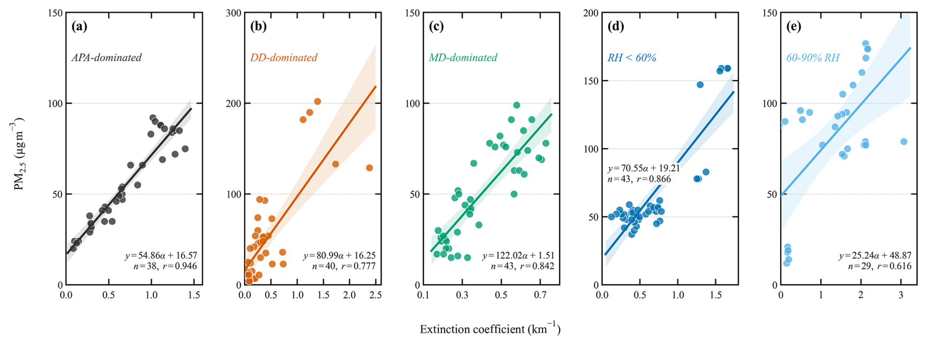
Figure 2 Relationships between PM_2.5 and the extinction coefficient under different aerosol-type and relative-humidity (RH) conditions. (a) APA-dominated samples; (b) DD-dominated samples; (c) MD-dominated samples; (d) samples without aerosol-type screening at RH<60 %; and (e) samples without aerosol-type screening at $\mathrm{60}\mathit{\%}<\mathrm{RH}<\mathrm{90}\mathit{\%}$. Shading indicates the 95 % confidence interval of the linear fit.

Figure 2 presents the fitting results between PM_2.5 and the extinction coefficient under different aerosol-type and humidity conditions. The linear relationship differs markedly among aerosol types and humidity regimes.

For APA events selected by aerosol classification (Fig. 2a), PM_2.5 and the extinction coefficient showed a strong linear correlation (r=0.946). The data points were concentrated, indicating that fine-mode pollution particles made relatively consistent contributions to extinction and PM_2.5 mass. This is therefore the main applicable condition for the linear retrieval model. In contrast, the correlation was weaker for DD-dominated cases (Fig. 2b; r=0.777), and the data were more dispersed. The MD-dominated samples (Fig. 2c; r=0.842) also showed a fitting relationship distinct from that of the APA-dominated samples. DD and MD are both dominated by nonspherical coarse-mode mineral particles. Their extinction contributions cannot be directly equated with their PM_2.5 mass contributions. At similar extinction values, the fitted PM_2.5 values under DD- or MD-dominated conditions were generally higher than those under APA-dominated conditions. Including mineral-aerosol extinction in model fitting could therefore introduce systematic bias. DD- and MD-dominated samples should consequently be excluded from the training dataset of the APA-constrained PM_2.5 retrieval model.

In addition to aerosol type, relative humidity also influences aerosol optical properties. The linear relationship between the extinction coefficient and PM_2.5 concentration was therefore compared under different humidity conditions without aerosol-type screening. The 60 % threshold was selected because enhanced hygroscopic growth over the North China Plain commonly becomes important at RH around this level (Liu et al., 2020; Petters and Kreidenweis, 2007); RH values above 90 % were excluded to avoid near-saturation conditions. These humidity groups were used only for the comparison in Fig. 2, rather than as aerosol-classification criteria. Under low-humidity conditions (RH<60 %; Fig. 2d), PM_2.5 and the extinction coefficient retained a positive correlation (r=0.866), but the data were more dispersed than under APA-dominated conditions. Under higher-humidity conditions ($\mathrm{60}\mathit{\%}<\mathrm{RH}<\mathrm{90}\mathit{\%}$; Fig. 2e), the correlation decreased to r=0.616. Hygroscopic growth at higher relative humidity can modify particle size, refractive index, and extinction efficiency. Because this process also depends on aerosol composition and particle loading, humidity screening alone cannot adequately constrain the correspondence between extinction and PM_2.5.

Figure 3 Comparison of ground-observed and model-retrieved PM_2.5 concentrations for the date-separated validation dataset: (a) Model A without an aerosol-type constraint; (b) Model B with PDR-only screening; and (c) Model C with combined PDR–G_f classification constraints. The dashed line denotes the 1:1 reference line. The annotations report the root mean square error (RMSE), mean absolute error (MAE), and mean bias (Bias).

Overall, Fig. 2 demonstrates that the extinction–PM_2.5 relationship depends on aerosol type and humidity conditions. The APA-selected samples show the most compact relationship, whereas DD-, MD-, and humidity-stratified samples without aerosol-type screening show greater dispersion or distinct fitting behaviour. These results demonstrate that total extinction or humidity screening alone cannot fully remove the influence of coarse-mode mineral aerosols. They therefore motivate the use of combined PDR–G_f aerosol-classification constraints, whose quantitative retrieval benefit is evaluated separately using the date-separated comparison of Models A, B, and C below.

To further assess the applicability of the three models to data outside their training dates, near-surface validation was conducted using 411 hourly samples from 69 observation dates that were excluded from model training. Figure 3 compares the PM_2.5 estimates from Models A, B, and C with the corresponding ground-based observations at the Wanliu station.

For Model A, the RMSE, MAE, and Bias were 28.04, 24.59, and 19.42 µg m⁻³, respectively. Without aerosol-type discrimination, extinction contributions from coarse-mode particles and mixed aerosols can be mapped to PM_2.5 mass concentration, resulting in an appreciable systematic overestimation. Model B, which used PDR-only screening, yielded an RMSE, MAE, and Bias of 25.42, 22.09, and 15.22 µg m⁻³, respectively. Although its errors were lower than those of Model A, a substantial positive bias remained, indicating that a single PDR condition cannot fully exclude mixed aerosols and low-depolarization particles with distinct optical properties.

Model C, which used combined PDR–G_f classification constraints, performed best, with an RMSE of 17.32 µg m⁻³, an MAE of 13.54 µg m⁻³, and a Bias of 3.30 µg m⁻³. Relative to Model A, the RMSE, MAE, and Bias of Model C decreased by 38.2 %, 45.0 %, and approximately 83.0 %, respectively. Relative to Model B, the RMSE and MAE decreased by 31.9 % and 38.7 %, respectively. The mean predicted concentration from Model C was 48.18 µg m⁻³, closer to the mean observed concentration of 44.88 µg m⁻³ in the validation dataset.

Overall, PDR-only screening can reduce the influence of non-APA aerosol components to some extent, but its discrimination capability remains limited. The addition of fluorescence capacity further distinguishes aerosols with similar depolarization characteristics but different optical properties, thereby reducing the inclusion of samples unsuitable for the PM_2.5 linear retrieval. These results show that the combined PDR–G_f classification constraint substantially reduces near-surface PM_2.5 reconstruction errors and systematic bias. These statistics quantify the near-surface performance of the empirical retrieval model and should not be interpreted as independent validation of the complete vertical PM_2.5 profiles.

Figure 4 Lidar-retrieved extinction coefficient profiles on 6 November 2024. The black solid line denotes the temporal median profile, and the gray shading represents the 25 %–75 % interquartile range. Panel (a) corresponds to 11:00–13:00 UTC, during which the extinction was mainly contributed by DD; panel (b) corresponds to 14:00–17:00 UTC, when APA gradually became dominant.

3.2 Influence of Aerosol Classification Constraints on PM_2.5 Retrieval Results

To demonstrate the influence of aerosol classification constraints on the retrieval of the vertical PM_2.5 structure, this section takes a typical mixed-aerosol pollution episode on 6 November 2024 as an example to analyze the characteristics of the extinction coefficient, the evolution of aerosol components, and the resulting differences in PM_2.5 retrievals.

As shown in Fig. 4, the median vertical profiles of the extinction coefficient during different periods exhibited pronounced differences in both magnitude and vertical distribution. During 11:00–13:00 UTC (Fig. 4a), the extinction coefficient varied relatively smoothly with height, without forming a distinct local maximum in the lower-to-middle layers. In contrast, during 14:00–17:00 UTC (Fig. 4b), the overall extinction coefficient increased markedly and showed a more concentrated enhancement at approximately 0.9–1.2 km.

To provide supplementary information on the vertical optical structure during this nighttime observation, Fig. S1 in the Supplement presents the full-nighttime median LR profile on 6 November 2024. Retrieved LR values were continuous between 0.45 and 1.50 km, indicating that lidar observations were available throughout this altitude range. The LR increased from approximately 20 sr near 0.45–0.60 km to a median value of 48.02 sr within 0.8–1.5 km, with an interquartile range of 44.84–50.54 sr. This pattern indicates distinct vertical optical stratification during the nighttime observation. The LR profile is provided only as Supplement on the vertical optical structure; it was not used as an aerosol-classification criterion or as an additional input to the PM_2.5 retrieval model. The 0.45–0.80 km interval was not excluded because of invalid data. Rather, the discussion focuses on 0.8–1.5 km because the identifiable PM_2.5 pollution-layer evolution in this case mainly occurred within that altitude range.

Although the above differences reflect changes in aerosol optical properties during different periods, the extinction coefficient itself still represents only the integrated contribution of aerosols with different particle sizes and compositions to optical extinction. Its variations may arise from an increase in fine-mode anthropogenic pollution aerosols, but may also be affected by the contribution of coarse-mode particles, such as dust. Under mixed-aerosol conditions, it is therefore necessary to further incorporate aerosol classification information to constrain the aerosol types corresponding to the extinction signal, so as to distinguish the actual contributions of different aerosol components to PM_2.5. Figure 5 shows the spatiotemporal variations in the aerosol component fractions during this period.

As shown in Fig. 5, during 11:00–13:00 UTC, both APA and dust aerosols contributed to extinction at different height levels, and their relative fractions varied markedly with altitude. After 14:00 UTC, the fraction of APAs increased rapidly and became dominant within the height range of 0.9–1.3 km. These results indicate that the aerosol components corresponding to the extinction coefficient were not consistent across different heights and time periods. If the extinction coefficient is directly used for PM_2.5 retrieval without component discrimination, the extinction contribution of coarse-mode particles can easily be misinterpreted as that of fine particulate pollutants, thereby introducing systematic biases.

The sensitivity of the component fractions to the adopted PDR and G_f end-member parameters is quantified by the Monte Carlo analysis in Sect. 3.3, and the resulting variability is propagated to the retrieved PM_2.5 estimates.

Figure 5 Time–height distributions of aerosol component fractions on 6 November 2024: (a) APA fraction; (b) DD fraction; and (c) MD fraction.

Figure 6 Vertical distributions of PM_2.5 retrieved with and without classification constraints and their differences during 11:00–13:00 UTC. (a) Median profiles and 25 %–75 % percentile ranges for the classification-constrained (Classified) and unconstrained (Unclassified) retrievals; (b) vertical profile of the difference between the two retrieval strategies, ΔPM_2.5, where the solid line denotes the median and the shading represents the 25 %–75 % percentile range. $\mathrm{\Delta }{\mathrm{PM}}_{\mathrm{2.5}}={\mathrm{PM}}_{\mathrm{2.5},\mathrm{unclassified}}-{\mathrm{PM}}_{\mathrm{2.5},\mathrm{classified}}$. The inset in panel (b) summarizes the paired differences over 0.8–1.5 km.

Based on the classification results shown in Fig. 5, Fig. 6 presents the vertical distributions of PM_2.5 retrieved with and without classification constraints, as well as their differences. Figure 6a compares the vertical profiles of PM_2.5 concentration retrieved during 11:00–13:00 UTC using the classification-constrained extinction coefficient and the extinction coefficient without classification constraints. The two retrieval results exhibited certain similarities in their vertical distribution patterns, both showing continuous structures varying with height, indicating that the vertical distribution of PM_2.5 during this period had a stable stratified structure. However, in terms of magnitude, the retrieval results without classification constraints were higher than the classification-constrained results throughout the entire height range. This difference is consistent with the overestimation tendency indicated by the fitting relationship under DD-dominated conditions in Sect. 3.1.

To further quantitatively compare the two retrieval strategies, valid paired time–height bins from the classification-constrained and unclassified retrievals were analyzed over 0.8–1.5 km during 11:00–13:00 UTC on 6 November 2024. The difference was defined as $\mathrm{\Delta }{\mathrm{PM}}_{\mathrm{2.5}}={\mathrm{PM}}_{\mathrm{2.5},\mathrm{unclassified}}-{\mathrm{PM}}_{\mathrm{2.5},\mathrm{classified}}$. As shown in Fig. 6b, the median ΔPM_2.5 was 20.8 µg m⁻³, with an interquartile range of 18.3–22.7 µg m⁻³; all paired differences were positive.

This result indicates that, during the mixed-to-pollution aerosol evolution event, the unclassified retrieval was systematically higher than the classification-constrained retrieval across the investigated time period and altitude range, rather than because of a few isolated heights or time steps. Together with the contribution of dust components to extinction during the early stage shown in Fig. 5, this stable positive difference indicates that, without distinguishing coarse-mode mineral particles from anthropogenic pollution particles, their extinction contribution may be mapped to PM_2.5 mass concentration. Introducing classification constraints can reduce this systematic effect.

3.3 Uncertainty and Sensitivity Analysis

To quantify uncertainties in mixed-component separation and linear retrieval, two mixed-aerosol pollution cases on 6 and 7 November 2024 were analyzed. The effects of classification end-member parameters, aerosol-type-dependent LR, extinction- coefficient measurement error, and linear-model parameters on the retrieved PM_2.5 were evaluated separately. Sensitivity to the assumed classification end-member parameters was quantified using 100 Monte Carlo perturbations of the pure-component PDR and G_f end-member parameters. The LR values for APA, DD, and MD were varied within the ranges listed in Table S1. The linear-model parameters were determined by bootstrap resampling with observation date as the resampling unit. The individual uncertainty sources and their joint propagation are summarized in Table S2.

For Model C, the bootstrap 95 % confidence intervals of the linear-model slope A and intercept B were 42.59–71.14 and 9.01–21.63, respectively. When only the classification end-member parameters were perturbed, the median widths of the 95 % PM_2.5 intervals were 2.40 and 2.76 µg m⁻³ for the two case days, respectively. When only aerosol-type-dependent LR was varied, the corresponding widths were 1.23 and 1.13 µg m⁻³. Under the low-LR, reference-LR, and high-LR scenarios, the median PM_2.5 estimates for the two case days ranged from 18.46 to 20.16 µg m⁻³ and from 18.59 to 20.45 µg m⁻³, respectively. These results indicate that changes in classification boundaries and component LR affect the quantitative PM_2.5 estimates but, within the plausible ranges considered here, do not alter the vertical structure of the major pollution layers.

When the classification-end-member, LR, extinction-coefficient measurement, and model-parameter uncertainties were jointly propagated, the median widths of the 95 % intervals for the mean PM_2.5 estimates were 12.02 and 12.79 µg m⁻³ for the two cases. After the training residual of the empirical linear model was additionally included, the median prediction- interval widths increased to 36.31 and 36.85 µg m⁻³, respectively. Thus, the dominant sources of uncertainty in the present retrieval are the scatter of the empirical extinction–PM_2.5 relationship and the stability of its fitted parameters, rather than perturbations of the classification end-member parameters or aerosol-type-dependent LR alone. The retrieved results are therefore interpreted as classification-constrained estimates with associated uncertainty ranges.

4 Discussion

4.1 Observation Background and Case Selection

To examine the physical plausibility of the vertical PM_2.5 distributions retrieved under aerosol classification constraints during actual pollution processes, this section selected observational data from 1 October to 30 December 2024 to analyze the overall background characteristics of pollution events in the study area. On this basis, representative typical episodes were further selected for discussion. The datasets included hourly ground-based PM_2.5 and PM₁₀ concentrations, the PM_2.5 $/$ PM₁₀ ratio, and relative humidity (RH) information obtained from radiosonde observations.

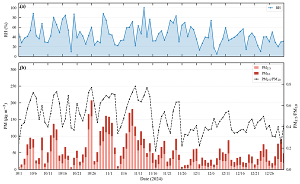
Figure 7 Ground-observed relative humidity from October to December 2024 (upper panel) and variations in particulate matter concentrations and ratios (lower panel).

Figure 7 shows that pollution events occurred frequently during the study period, with PM_2.5 and PM₁₀ exhibiting multiple episodic increases. During most pollution episodes, the PM_2.5 $/$ PM₁₀ ratio was higher than 0.5, indicating that fine-mode pollution aerosols dominated the overall pollution processes. In contrast, the ratio decreased markedly during some periods, suggesting an enhanced contribution from coarse-mode particles, such as dust or resuspended dust. Relative humidity fluctuated substantially during the study period, and most pollution episodes were accompanied by increases in humidity, indicating that aerosol hygroscopic growth may have been involved in the evolution of particulate optical properties and pollution processes.

Based on the above background characteristics and aerosol classification results, 6–7 November was selected as a typical case for analysis in this study. 6 November represented a typical mixed-aerosol pollution process, during which dust and pollution aerosols exhibited pronounced vertical stratification and mixing. In contrast, 7 November was dominated by APAs, with pollution concentrations remaining at a persistently high level. Together, these two days constituted a continuous evolution process from mixed aerosols to APAs, which can be used to evaluate the applicability and physical consistency of the classification-constrained retrieval method under different aerosol backgrounds.

4.2 Mixed Aerosol Case

The 6 November case was used to examine the physical plausibility of the retrieved PM_2.5 structure under mixed-aerosol conditions. Aerosol types and component fractions were calculated using the δ_p–G_f method (Fig. 5). During 11:00–13:00 UTC, DD dominated the middle-to-upper layer at 1.1–1.5 km. After 13:30 UTC, the APA fraction increased rapidly and became dominant. The case therefore evolved from dust-dominated to pollution-aerosol-dominated conditions.

The APA-related extinction coefficient was then extracted using the component-separation method in Sect. 2. It was used as input to the linear model in Sect. 3 to retrieve the spatiotemporal PM_2.5 distribution (Fig. 8).

Figure 8 Spatiotemporal distribution of lidar-retrieved PM_2.5 concentration on 6 November 2024.

Figure 8 shows stage-dependent changes in the PM_2.5 structure. During 14:00–15:00 UTC, a high-PM_2.5 region developed at 0.8–1.2 km, and concentrations increased from approximately 25 to 35 µg m⁻³. The layer was about 0.4 km thick. During 15:00–17:00 UTC, the layer intensified and expanded upward. Its upper boundary rose from approximately 1.2 to 1.35 km and its thickness increased to approximately 0.55 km. Peak concentrations of 42 µg m⁻³ occurred near 1.2–1.3 km. This development coincided with the rapid increase in APA fraction and occupied a similar height range (0.8–1.4 km). The retrieval therefore captured the compositional transition of the pollution layer.

To analyze the thermodynamic background of the pollution-layer evolution, temperature profiles, vertical temperature gradients, and the pollution-layer height (PLH) are presented in Fig. 9.

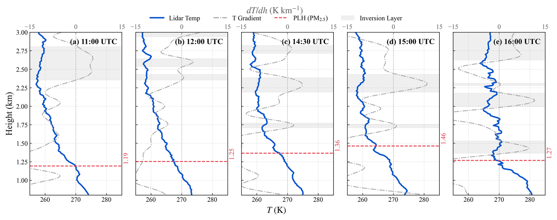
Figure 9 Temperature profile (blue line) and vertical temperature lapse rate profile (gray dash-dotted line) on 6 November 2024. The red dashed line marks the PLH, and the gray shading denotes the inversion layer. The downward extension of the inversion layer was consistent with the thickening and upward development of the retrieved PM_2.5 layer shown in Fig. 8.

During 11:00–12:00 UTC, the inversion layer was located above 2.3 km and exerted only a weak constraint on the lower pollution layer. The PM_2.5 layer top was then 1.19–1.25 km and concentrations were relatively low. After 14:30 UTC, the inversion layer strengthened and extended downward. Its lower boundary reached 1.4–1.5 km during 15:00–16:00 UTC. At the same time, PM_2.5 accumulated within 0.8–1.4 km and the layer top rose to 1.36–1.46 km. The evolution of the pollution layer was therefore consistent with strengthened stable stratification, which can suppress vertical turbulent exchange and favor pollutant accumulation.

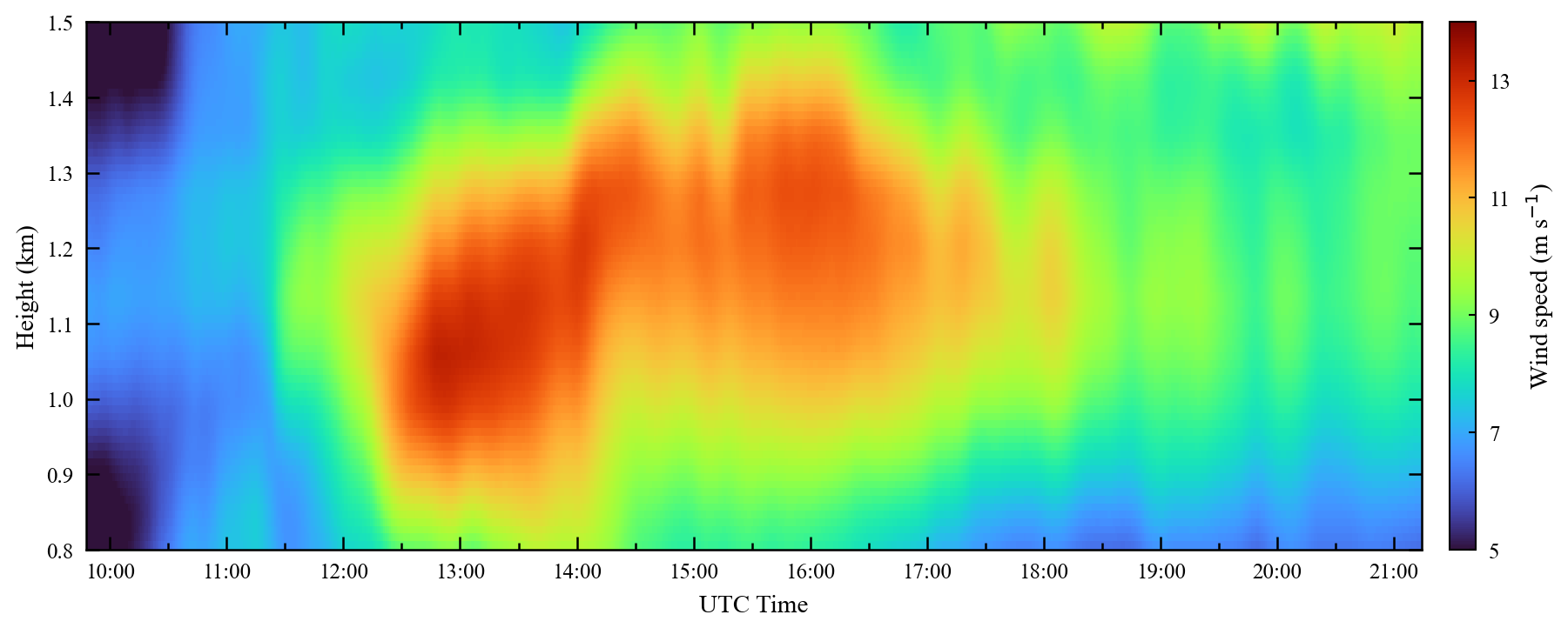
During 11:00–12:00,UTC, winds above 1.1 km were weak (6–8 m s⁻¹) and mainly northwesterly (250–270°). This pattern was consistent with the elevated DD fraction in the middle-to-upper layer. Below 1.1 km, wind speeds increased from 8–10 to 13–15 m s⁻¹ after 13:00 UTC. The wind direction remained within 230–250°, forming a low-level transport pathway. This change coincided with the rapid increase in the APA fraction.

Figure 10 Time–height evolution of wind speed on 6 November 2024 during 11:00–18:00 UTC.

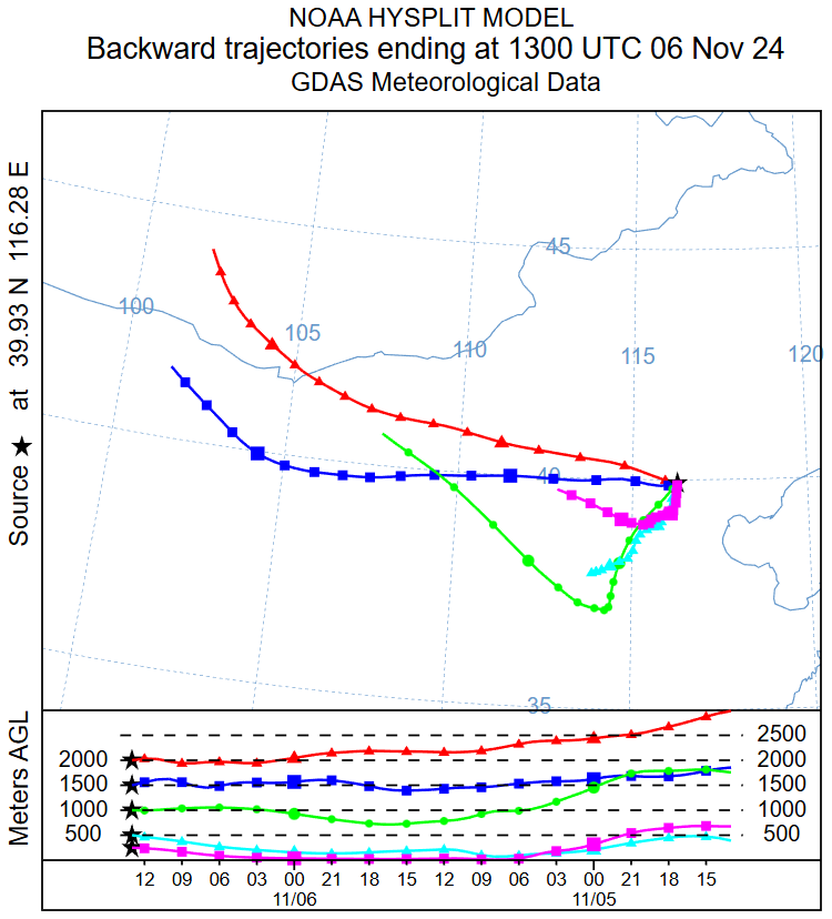
Figure 11 Backward trajectories starting from Beijing at 13:00 UTC on 6 November 2024.

Backward trajectories at 13:00 UTC (Fig. 11) further distinguished the air-mass sources. Air masses at 1.5–2.0 km originated mainly from the Mongolian Gobi and desert regions of Inner Mongolia and descended before reaching Beijing. Air masses at 0.5–1.5 km originated mainly from industrial and urban regions in the southwestern North China Plain. These altitude-dependent source regions were consistent with the DD aloft and the lower-level pollution layer.

Figure 12 Spatiotemporal distribution of lidar-retrieved PM_2.5 concentration on 7 November 2024.

4.3 APA Case

The case on 7 November was used to analyze the evolution characteristics of the vertical PM_2.5 structure under APA-dominated conditions and to examine the applicability of the classification-constrained retrieval method in an anthropogenic-pollution-aerosol background. This episode occurred after the mixed-aerosol stage on the previous day, when the influence of DD and MD transport had weakened markedly. Aerosols in the lower layers were dominated by APAs, and PM_2.5 concentrations at the surface and in the near-surface layer remained persistently high.

Figure 12 shows the spatiotemporal distribution of lidar-retrieved PM_2.5 concentration on 7 November. The pollution layer showed distinct stages within the 0.8–1.5 km height range. During 10:00–11:30 UTC, the high-concentration region was mainly located at 0.8–1.2 km. Its top was 1.3–1.4 km and concentrations were 60–78 µg m⁻³. By 13:20 UTC, the layer top had descended to approximately 1.11 km, indicating compression and weakening. After 17:00 UTC, PM_2.5 increased and expanded upward again. By 19:30 UTC, the layer top had risen to approximately 1.46 km and peak concentrations reached 80–85 µg m⁻³. After 20:00 UTC, the layer remained at a relatively high concentration level.

Figure 13 Temperature profile (blue line) and vertical temperature gradient profile (gray dash-dotted line) on 7 November 2024. The red dashed line indicates the PM_2.5 PLH, and the gray shading denotes the inversion layer. Temporal changes in inversion-layer height were consistent with the compression and subsequent upward development of the retrieved PM_2.5 layer shown in Fig. 12.

It should be noted that the pollution-layer height (PLH) determined from the lidar-derived PM_2.5 profiles represents the upper boundary of the pollution aerosol layer and is not equivalent to the meteorological boundary-layer height (BLH). Hourly ERA5 BLH values during the nighttime periods corresponding to Figs. 8 and 12 were mainly 0.015–0.024 km, well below the lower displayed altitude of 0.8 km in the PM_2.5 time–height plots. ERA5 BLH was therefore neither overlaid on these figures nor used as a surrogate for PLH; the vertical evolution of the pollution layer was instead interpreted using temperature gradients, inversion-layer structure, wind fields, and the lidar-derived PLH. At 10:40 and 11:20 UTC, the inversion layer was located at 1.4–1.7 km, while the PM_2.5 layer tops were 1.33 and 1.41 km, respectively. At 13:20 UTC, both the inversion layer and pollution layer were depressed, and the PM_2.5 layer top decreased to 1.11 km. At 19:30 UTC, the pollution layer top rose to 1.46 km with the elevated inversion layer. At 20:20 UTC, the stable lower-layer structure persisted and the layer top remained approximately 1.33 km. Overall, the PM_2.5 layer top was generally located near the base of the stable stratification, indicating strong thermodynamic control of its vertical evolution.

During 10:00–11:30 UTC, wind speeds at 0.8–1.3 km were weak (5–8 m s⁻¹), while the pollution layer was relatively thick. From 12:00 to 17:00 UTC, wind speeds increased to 10–14 m s⁻¹. The high-PM_2.5 region then contracted and the layer top descended. After 17:00 UTC, winds weakened and PM_2.5 increased again, accompanied by an upward expansion of the layer. Together with the temperature profiles, these results indicate that stronger winds favored layer compression, whereas weaker winds and persistent stable stratification favored pollutant re-accumulation.

Figure 14 Time–height distribution of wind speed on 7 November 2024.

4.4 Applicability and Limitations of the Classification-Constrained Model

The chemical composition and sources of PM_2.5 in Beijing exhibit pronounced seasonal variability. Previous observations have shown that the concentrations and relative contributions of secondary inorganic ions, carbonaceous components, and crustal elements vary among seasons. Stronger photochemical processes in summer favor secondary inorganic aerosol formation, carbonaceous components and combustion emissions have relatively stronger influences in autumn and winter, and dust events and crustal materials are more important in spring and autumn (Zhao et al., 2013; Sun et al., 2015; Han et al., 2020). These changes can modify particle extinction efficiency, hygroscopic-growth behavior, and mass extinction efficiency, thereby affecting the empirical relationship between extinction coefficient and PM_2.5. It is therefore necessary to examine the applicability of the present model under different seasonal conditions.

Accordingly, season-specific models were constructed for spring, summer, autumn, and winter using date-separated training and validation samples, and their results were compared with those of the all-season Model C for the corresponding seasonal validation data (Table S3). Season-specific fitting did not yield a stable and consistent performance improvement. The RMSE values of the season-specific models in spring, autumn, and winter were 18.96, 14.22, and 20.18 µg m⁻³, respectively, comparable to or higher than those of the all-season Model C (18.19, 14.01, and 15.30 µg m⁻³). Although the summer RMSE decreased from 21.49 to 16.38 µg m⁻³, the available sample size was limited and the fitted relationship was unstable. Thus, the present results do not support the establishment of a universally applicable set of fixed seasonal parameters.

To examine the relationship between the DD and MD classification results and ground-level coarse-particle pollution, an exploratory date-separated linear regression was performed between the hourly mean extinction coefficient at 0.45–0.60 km during DD/MD-classified periods and ground-level PM₁₀ (Table S4). The model was fitted using 48 training samples and evaluated using 309 independent hourly samples. The validation showed a weak relationship (r=0.31), with an RMSE of 104.61 µg m⁻³, an MAE of 88.98 µg m⁻³, and a positive bias of 69.11 µg m⁻³. This limited performance likely reflects the variable mass-extinction efficiency of coarse mineral particles, the vertical representativeness difference between the lidar layer and surface observations, and the unbalanced numbers of DD, MD, and DD–MD mixed samples. Therefore, a stable quantitative PM₁₀ retrieval relationship was not obtained. Ground-level PM₁₀ is therefore used only as auxiliary consistency information in this study, rather than as direct quantitative validation of the DD/MD classification results.

The APA class in this study describes pollution aerosols with similar PDR and fluorescence characteristics rather than particles with a fixed chemical composition. Because synchronous chemical-composition observations were unavailable, the relative contributions of sulfate, nitrate, organic components, black carbon, and hygroscopic growth to changes in the fitted model parameters could not be quantified. Model C is therefore positioned as an empirical retrieval model for local APA conditions in Beijing. When applied to other regions, seasons, or pollution conditions with substantially different aerosol composition, its parameters should be recalibrated using local PM_2.5 and optical observations.

4.5 Section Conclusion

Based on ground-level particulate matter concentrations, the PM_2.5 $/$ PM₁₀ ratio, and relative humidity from October to November 2024, this section analyzed the overall background of pollution processes during the study period. The period of 6–7 November was selected as a typical case, and the evolution characteristics of the vertical PM_2.5 structure during a mixed-aerosol process and an APA-dominated pollution process were discussed separately. The case on 6 November indicates that this process exhibited distinct stratification and evolution characteristics of mixed aerosols. In the early stage, DD dominated the middle-to-upper layers, after which the APA fraction increased rapidly, and the retrieved high-PM_2.5 region gradually developed and intensified within the 0.8–1.4 km height range. Combined analyses of temperature stratification, wind speed distribution, and backward trajectories showed that the strengthening and downward extension of the inversion layer, changes in transport conditions in the middle-to-lower layers, and differences in air-mass origins at different altitudes were generally consistent with the formation and uplift of the pollution layer. The case on 7 November shows that, under APA-dominated conditions, the vertical PM_2.5 structure exhibited stage-dependent variations characterized by initial compression followed by subsequent development. Temperature profile analysis showed that the pollution layer top was generally located near the base of the stable stratification or at a comparable altitude. Wind speed variations further indicated that stronger wind speeds in the middle-to-lower layers corresponded to compression of the pollution layer, whereas weakened winds accompanied by the persistence of a stable layer favored the re-thickening and upward development of the pollution layer. Overall, both typical cases demonstrate that the classification-constrained retrieval results of the vertical PM_2.5 distribution can reasonably reflect the structural evolution of pollution layers under different aerosol backgrounds and remain generally consistent with independent changes in thermodynamic and dynamical conditions, thereby supporting the physical plausibility and applicability of this method under mixed-aerosol and evolving pollution conditions.

5 Conclusions

This study developed a lidar-based method for retrieving the vertical structure of PM_2.5 under classification constraints. By incorporating component constraints into both model development and application, the applicable conditions of the empirical extinction–PM_2.5 relationship were clarified and the interference of non-APA aerosol components under mixed-aerosol conditions was reduced. Analysis of a mixed-to-pollution aerosol evolution process in Beijing in November 2024 showed that, during the coexistence of dust and APA, the height of the classification-constrained high-PM_2.5 layer was consistent with the aerosol component distribution, low-level transport pathways, and stable-stratification structure. During the APA-dominated stage, the enhancement, compression, and subsequent uplift of the PM_2.5 vertical structure were consistent with changes in temperature stratification and wind fields. These results show that classification constraints reduce the influence of non-APA aerosol components on the quantitative PM_2.5 estimates and support the physical interpretation of the vertical structure during mixed-aerosol and evolving pollution processes.

Near-surface validation using matched samples from dates excluded from model training showed that Model C, constrained by combined PDR–G_f classification, performed best. Its RMSE, MAE, and Bias were 17.32, 13.54, and 3.30 µg m⁻³, respectively, representing reductions of 38.2 %, 45.0 %, and approximately 83.0 % relative to the model without an aerosol-type constraint. Compared with the PDR-only model, the RMSE and MAE were reduced by 31.9 % and 38.7 %, respectively. These results indicate that PDR screening can partly reduce the influence of non-APA aerosol components, whereas the additional optical information provided by G_f further improves the selection of samples appropriate for the empirical PM_2.5 retrieval.

The uncertainty analysis showed that perturbations of classification end-member parameters and aerosol-type-dependent LR values affect PM_2.5 estimates under mixed-aerosol conditions, but the dominant prediction uncertainties arise from scatter in the empirical extinction–PM_2.5 relationship and the stability of the fitted parameters. Seasonal testing did not show a stable and consistent improvement from season-specific fitting, indicating that the current model should be regarded as an empirical relationship for local APA-dominated conditions in Beijing.

This study has several limitations. The ground-station comparison evaluates consistency between the 0.45–0.60 km lidar layer and surface PM_2.5 observations; it does not replace direct in situ validation of the complete vertical PM_2.5 profile. In addition, observations of PM_2.5 at multiple heights, humidity profiles, and synchronous chemical composition were unavailable, limiting the quantification of the environmental dependence of classification thresholds, component LR values, and the mass-conversion relationship. Future work should combine tethered-balloon, unmanned aerial vehicle, or aircraft observations with local chemical-composition and optical measurements to validate the vertical retrievals and calibrate model parameters for different regions, seasons, and pollution conditions.