Airborne performance assessment of the DLR MIRO MGA³ quantum cascade laser spectrometer for fast N₂O measurements

Nitrous oxide (N₂O) is the most dominant precursor of ozone-depleting substances and the third most important anthropogenic greenhouse gas, with agriculture contributing the largest share of emissions (56 %). Over the past two decades, airborne in-situ measurements have become increasingly important for studying emission and transport of N₂O in the atmosphere, also driven by the development of more precise and simultaneously faster Quantum Cascade Laser (QCL)-based spectrometers.

However, many QCL-based spectrometers exhibit sensitivities to environmental and flight-related parameters that can vary rapidly (≤ 1 s), such as static or cabin pressure and aircraft roll and pitch angles. The impact of changing ambient water vapor is particularly critical due to both dilution and quantum-mechanical effects. Because the variability of N₂O in the lower troposphere is often very small (< 1 ppb) relative to its high background (∼ 338 ppb), even minor variations in these parameters can significantly affect data quality and must be corrected. Although many instruments can resolve such small concentration changes, their typical temporal resolution of 1 Hz may limit the application of advanced measurement techniques such as eddy covariance on fast-moving aircraft.

Here, we present and evaluate a new instrument setup for precise (< 0.2 ppb) and high-frequency (10 Hz) airborne in-situ N₂O measurements in altitudes up to 4500 m based on a MIRO MGA³ QCL spectrometer (MIRO Analytical AG). The instrument was successfully deployed during two airborne science missions, namely onboard the unpressurized DLR Cessna during the Greenhouse Gas Monitoring (GHGMon) campaign in 2023 in the Netherlands, as well as onboard the NASA DC-8 during the Airborne and Satellite Investigation of Asian Air Quality (ASIA-AQ) campaign in 2024. Specifically, we evaluate and compare different water vapor correction approaches using ASIA-AQ data sampled within the tropical boundary layer over South Korea, the Philippines, Thailand and Taiwan, which partly were characterized by specifically high ambient humidity (up to 30 000 ppm H₂O). The water vapor correction methods include an empirical approach that relies on both native and corrected MIRO in-flight water vapor measurements, as well as an approach by an updated version of the MIRO specific fitting software. Comparison with N₂O measurements from a well-established instrument onboard the NASA DC-8 shows agreement within combined measurement uncertainties for all tested water vapor correction approaches, albeit special caution is needed for humidities larger than 15 000 ppm. The new water vapor corrected data shows a 42 % better precision than with original default settings of the instrument. We further show that the instrument setup is insensitive to flight parameter changes such as roll and pitch angle of the aircraft, and allows for stable measurements even under challenging conditions such as in the turbulent boundary layer.

This instrument setup enables improved characterization of N₂O emissions and sources from the agricultural sector, which is particularly relevant for tropical regions with strong agricultural activity and high humidity, where observational data remain scarce.

1 Introduction

Nitrous Oxide (N₂O) is, after carbon dioxide (CO₂) and methane (CH₄), the third most important anthropogenic greenhouse gas (GHG) (Myhre et al., 2013) and the dominant precursor of ozone (O₃)-depleting substances in the stratosphere (Ravishankara et al., 2009). It has an atmospheric lifetime exceeding 100 years (Prather and Wilson, 2026; Prather et al., 2023, 2015; Myhre et al., 2013). Since the preindustrial era, its atmospheric mole fraction has increased from approximately 270 ppb in 1750 to 336 ppb in 2022 (Tian et al., 2024; MacFarling Meure et al., 2006) corresponding to a sustained rise with a mean annual growth rate of 0.96 ppb yr⁻¹ during the decade from 2010 to 2019 (Tian et al., 2024).

N₂O is emitted to the atmosphere from both natural (65 % of total net emissions) and anthropogenic (35 %) sources (Tian et al., 2024). Among anthropogenic sources, agriculture dominates, accounting for 56 % of total net emissions. These emissions primarily arise from the microbial processes of nitrification and denitrification, through which organic and synthetic fertilizers are partially converted to N₂O, as well as from direct nitrogen (N) inputs to soils (Tian et al., 2024; Smith, 2017). Additional significant anthropogenic contributions originate from other direct emissions (32 %), including industry, fossil fuel use, and biomass burning (Tian et al., 2024). The growth rate is expected to increase even further in the future due to the growing demand for food, energy and industrial processes associated with continued population growth (Tian et al., 2024; Smith, 2017; Reay et al., 2012).

This makes N₂O a key target for future mitigation policy (Kanter et al., 2020). To meet the goals of the Paris Agreement (UNFCCC, 2018), limiting global warming to 2 °C requires a reduction in N₂O emissions of 11 % by 2050 and as much as 22 % to achieve the 1.5 °C limit (Rogelj and Lamboll, 2024; Tian et al., 2024). However, alarmingly, even the worst case Representative Concentration Pathways (RCPs) and Shared Socioeconomic Pathways (SSPs) underestimate the global mean N₂O mole fractions observed in the atmosphere by roughly 2–3 ppb in 2020 (Tian et al., 2024). Current models sometimes lack adequate representation for N₂O emission factors, for example, for the amount of N soil input or freeze-thaw cycles, which results from a lack of data and measurements for specific regions (Del Grosso et al., 2022; Thompson et al., 2019).

Developing efficient mitigation strategies requires precise quantification of emissions from dominant source sectors and a robust understanding of the underlying processes. N₂O emissions can be estimated using a range of approaches, commonly classified as Bottom Up (BU) and Top Down (TD) methods (Tian et al., 2024; Saboya et al., 2024; CCAC, 2024; Davidson and Kanter, 2014). TD approaches include satellite observations, which offer global coverage but are not yet operational for N₂O (Kiemle et al., 2024). At smaller scales, chamber and tower measurements provide insights at spatial extents of 1 m² and up to 10 km², respectively, but are inherently limited to fixed locations (Chadwick et al., 2014; Rapson and Dacres, 2014; Pattey et al., 2007). In contrast, airborne measurements can cover regional scales on the order of 1–100 km and help bridge spatial gaps in the data from chamber and tall tower measurements (Dacic et al., 2024; Pattey et al., 2007). Additionally, in combination with eddy covariance techniques, they further enable improved quantification of emissions from specific sources, which is particularly valuable for the complex and heterogeneous agricultural sector (Waldmann et al., 2026; Smith, 2017).

In the case of N₂O, previously used instruments for high precision N₂O measurements, such as the well established Gas Chromatographs (GCs) or Fourier transform infrared (FTIR) spectrometers with temporal resolutions in the order of 1 min, are being replaced due to the improvement of laser-based measurement techniques and the growing commercial availability of laser spectrometers, allowing for precise (< 1 ppb) and simultaneously faster measurements (∼ 1 Hz) (CCAC, 2024; Lebegue et al., 2016; Rapson and Dacres, 2014; Lopez et al., 2012). Particularly, the development of Continuous Wave (CW) Quantum Cascade Lasers (QCLs) working at room temperature opened new possibilities for fast, continuous, more sensitive and more feasible mid-Infrared (IR) absorption spectroscopy (Li et al., 2013; Capasso, 2010) making overly complicated and expensive cooling systems on an aircraft redundant.

Several airborne N₂O in-situ studies using QCLs or other laser-based techniques have already been successfully conducted over the last two decades (Dacic et al., 2024; Eckl et al., 2021; Gvakharia et al., 2020; Kostinek et al., 2019; Gvakharia et al., 2018; Pitt et al., 2016; Xiang et al., 2013; Schiller et al., 2008). However, many of these studies report a temporal resolution of 1 Hz or less, which can be too slow for N₂O eddy covariance measurements on a fast aircraft. Furthermore, airborne measurements still bear more challenges than ground based measurements. During a flight, several parameters may vary considerably, thereby affecting measurement performance. Pitt et al. (2016), Gvakharia et al. (2018) and Kostinek et al. (2019), for example, report dependencies on changes in cabin pressure, roll and pitch angles of the aircraft, and also water vapor (H₂O), which resulted in deviations of some ppb in N₂O. This can be difficult for the precise measurement of small N₂O variability (< 1 ppb) and could be particularly problematic for flights in highly humid regions. Therefore, possible dependencies must be known and addressed by empirical corrections and specific calibration procedures. Furthermore, the space for the instrument setup onboard the aircraft is usually limited, resulting, e.g., in fewer possibilities to carry calibration gases which can impact the calibration procedure and, consequently, data quality.

Here, we present the performance assessment and evaluation of the DLR-MIRO system, a fast (10 Hz sampling frequency) airborne measurement setup specifically tuned for N₂O measurements with an in-flight precision of ∼ 0.18 ppb enabling airborne eddy covariance measurements for N₂O (Waldmann et al., 2026). The core instrument of the setup is a commercially available Quantum Cascade Laser Absorption Spectrometer (QCLAS), namely a Multicompound Gas Analyzer (MGA³), from the Swiss company MIRO Analytical AG. We assess the performance of the instrument during in-flight operation onboard two different research aircraft, a Cessna 208-B Grand Caravan operated by the German Aerospace Center (DLR) with an unpressurized cabin and NASA's Douglas DC-8 with a pressurized cabin. The Cessna was deployed on the Greenhouse Gas Monitoring (GHGMon) campaign in the Netherlands in June 2023. The DC-8 was deployed on the NASA Airborne and Satellite Investigation of Asian Air Quality (ASIA-AQ) campaign in February and March 2024 over the Philippines, South Korea, Taiwan and Thailand. Flights were conducted in humid regions using repeated country-specific flight patterns and vertical profiles. Due to the high variability of H₂O (0 %–3 %) in tropical environments, we focus on its impact on retrieved N₂O mole fractions. This is particularly important because the original fitting software version v1 did not account for H₂O effects, including both dilution and quantum-mechanical processes such as line broadening. To address this, we derive an empirical water vapor correction based on dedicated laboratory experiments. The results obtained with this correction are compared with those from an updated MIRO fitting software v2, which incorporates a water vapor correction derived from the same experimental dataset from the laboratory. We evaluate and discuss the advantages and limitations of both approaches, including an assessment of the MGA³ H₂O measurements themselves and the importance for their overall accuracy.

This study is structured as follows: in Sect. 2, we present the specifications of our MGA³ instrument and the airborne setup, which was identical for both the NASA DC-8 and the DLR Cessna Grand Caravan. We describe the calibration procedure, the basics of the retrieval software v1 of the MGA³ and elaborate on the relevant parameters for fitting the measured spectra, such as the width of absorption line (β). In Sect. 3, we first provide an overview of the different water vapor correction approaches applied in this study and describe the laboratory experiment used to derive corresponding parameters for the correction equation. In the next step, we compare the MGA³ H₂O-measurements to NASA's established Diode Laser Hygrometer (DLH) H₂O-measurements to derive an even more precise water vapor correction. We compare our empirical water vapor correction approaches with a new software version v2 that already implements a water vapor correction based on the same conducted laboratory experiment. We also compare our H₂O-corrected N₂O-measurements with N₂O-measurements conducted by NASA's established Differential Absorption Carbon monOxide Measurements (DACOM) spectrometer (Sachse et al., 1987), a Tunable Diode Laser Absorption Spectrometer (TDLAS) which was also onboard the DC-8 during the ASIA-AQ campaign. In Sect. 4, we assess the stability of the MGA³ under ground conditions by calculating its Allan precision and investigate potential dependencies of N₂O-measurements on cabin pressure and roll and pitch angles of the aircraft during flights. In Sect. 5, we present selected flight data from the ASIA-AQ campaign corrected using the different water vapor correction approaches. Finally, we show examples of ambient N₂O measurements from GHGMon and ASIA-AQ to demonstrate the capabilities of the MGA³ airborne setup under in-flight conditions.

2 Operational Design

At both the GHGMon and the ASIA-AQ campaign, we operated the same DLR-MIRO setup with a commercially available QCLAS, namely the Multicompound Gas Analyzer (MGA³) by the MIRO Analytical AG from Switzerland, as its core instrument. The setup is specifically optimized for N₂O measurements with the capability for the eddy covariance method and up to altitudes of approximately 5.5 km. In the following sections we first describe the specifications of the MGA³, its integration into the airborne instrument setup, and the data calibration procedure. To provide a better context for our water vapor correction approach, Sect. 2.4 and 2.5 outlines the basic theory of spectral fitting and introduces the most important parameters for the water vapor correction as well as the method used by the MGA³ mole fraction retrieval software.

2.1 Instrument specifications of the MIRO MGA³

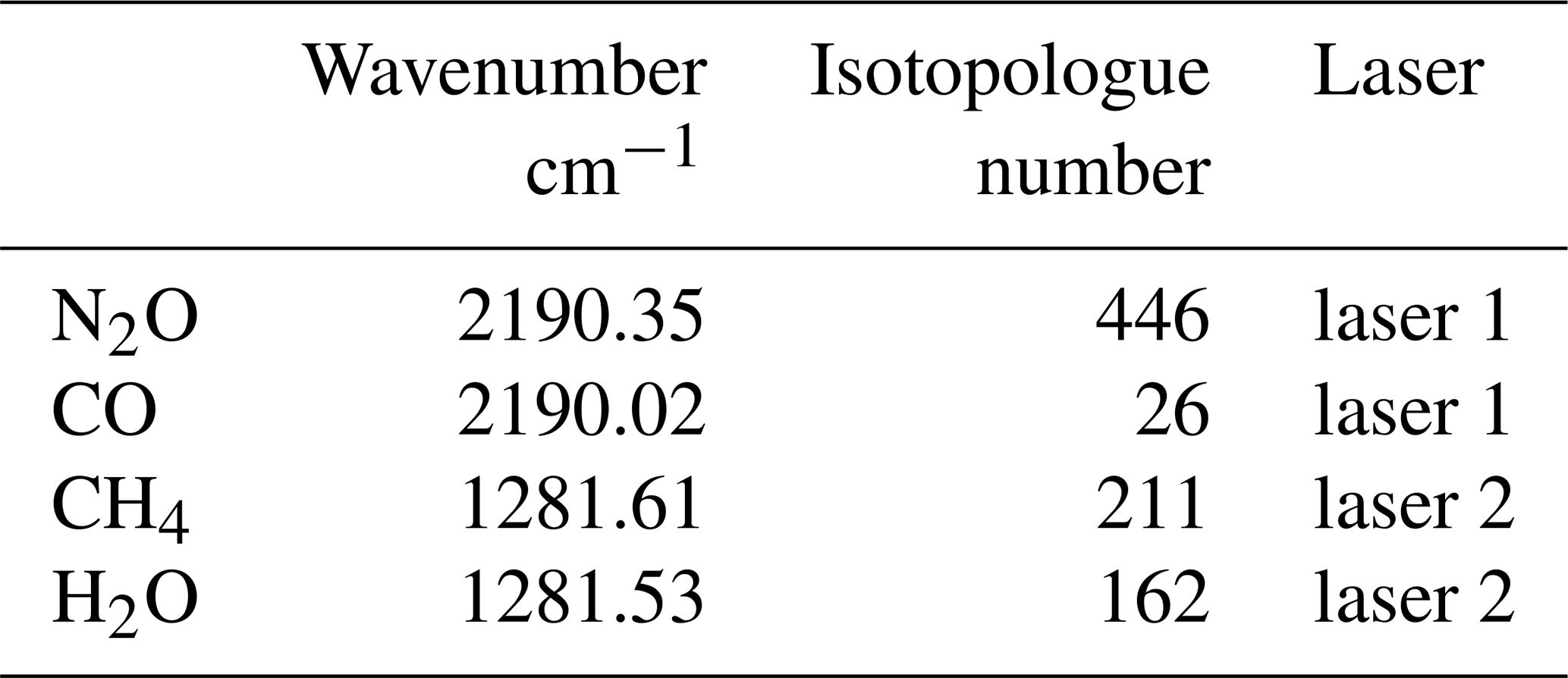
The MGA³ is a two-laser (Alpes Lasers; St. Blaise, Switzerland) QCLAS and is able to measure three species at once – N₂O, CH₄, and CO – in addition to H₂O, all within one Herriot measurement cell with a volume of 0.44 L and an optical path length of 76 m. The wavenumbers scanned by the first laser (laser 1) are 2191.38–2189.85 cm⁻¹ and the wavenumbers of the second laser (laser 2) are 1282.50–1281.01 cm⁻¹ (see Table 1). The MGA³ is specifically optimized for N₂O measurements by the selection of the spectral absorption lines and the settings defined by the manufacturer. The maximum time resolution of the data retrieval of the instrument is 10 Hz.

Table 1 Wavenumbers and HITRAN isotopologue numbers of the absorption lines of the target species of laser 1 and laser 2 of the MGA³.

The QCLs are driven by an intermittent Continuous Wave (iCW) driving scheme with pulse durations of 10–100 s and an overall period of about 0.5–1 ms. The temperatures of the lasers are held constant at around 32 °C (laser 1) and −2 °C (laser 2) by ThermoElectric Coolers (TECs). For further general information on the MGAs by MIRO Analytical, please find the paper of Hundt et al. (2018).

2.2 Airborne setup

For the complete functional airborne setup, the MGA³ requires additional structural components and peripheral devices. First, a liquid chiller (Thermorack401, Solid State Cooling Systems, Wappingers Falls, USA) provides the heat reservoir for the optical compartment of the MGA³ and the TECs cooling the lasers within the compartment (see Sect. 2.1) as can be seen in Fig. 1. The MGA³ has two inlets, one sample air inlet and one calibration gas inlet. When measuring sample air from outside the DC-8 aircraft, the air is first drawn through a rear-facing 62° trapezoid inlet at the hull of the aircraft and then directed through an about 6.5 m long PTFE tube with a diameter of $\mathrm{1}/\mathrm{2}$ in. to a 2 µm PTFE-membrane particle filter (filter membrane: R2PJ047 Pall, filter holder: PA1235 Pall). For the Cessna, the PTFE tube was approximately 5.5 m long and installed through the wing of the aircraft and through its attached wingpod. After filtering the sample air passes a Mass Flow Meter (MFM) (F-102E, Bronkhorst) before it enters the MGA³ through its sample air inlet. A scroll pump (IS500C, Anest Iwata) connected to the outlet of the MGA³ is used for creating a vacuum which draws the sample air in. The pump was specifically selected to generate the highest possible mass flow without exceeding the Cessna's power constraints. In this instrument setup with the long inlet tubing, the pump generated a mass flow of 12.5–13.8 slpm. The pump motor is additionally cooled with a standard external fan to prevent overheating. Given the MGA³ cell volume of 0.44 L and a cell pressure of 70 hPa this corresponds to an effective sampling frequency of 6.85–7.57 Hz, assuming plug flow. To achieve higher mass flows, and therefore higher effective sampling frequencies, we recommend minimizing the distance between the aircraft inlet and the instrument.

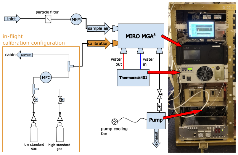
Figure 1 Setup of the instrumentation for both the 2023 GHGmon campaign and the 2024 ASIA-AQ campaign. The left side shows a scheme of the setup including the calibration setup within the orange box. The right side contains a photo of the setup onboard NASA's DC-8 during ASIA-AQ.

2.3 Calibration of data and response time

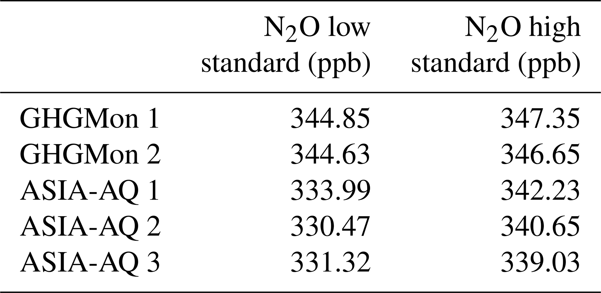
In this section, we describe the calibration procedure applied to our data to account for drifts and potential changes in the sensitivity of the MGA³ and determine the response time of the system. To avoid drift and sensitivity effects of GHG measurements and to improve the accuracy of the retrieved mole fractions, the instrument needs to be regularly calibrated in-flight using a two-point calibration. For this, the MGA³ switches an internal valve and then draws air not from the sample air inlet but from the calibration gas inlet which is connected to an in-flight calibration system (see Fig. 1, orange box). As can be seen from the measurements in Fig. 2, as an example from ASIA-AQ, every 10 min two calibration gases are drawn, a low-standard calibration gas L and a high-standard calibration gas H, each for 20 s in sequence. Two solenoid valves are operated directly from the MGA³ software and they control which of the two gases is currently being used. The red areas show the L and H standards, and the grey areas show when cabin air is sampled through the overflow while switching the main MGA³ valve from the sample air inlet to the calibration gas inlet. When the main valve of the MGA³ switches to cabin air in the first gray area or when the solenoid valves switch to the calibration gases, the initial high pressure coming from the cabin or the cylinders results in a feedback behavior leading to a time of 1–2 s for the cell to be completely flooded by the cabin air or the calibration gases. When switching the valves back to the cabin air in the second grey area in Fig. 2 or back to ambient sampling air after the second red area, this effect does not occur. With these two cases we determine our response time of 0.1–0.2 s which confirms our effective sampling frequency of approximately 7 Hz determined with the mass flow through the cell in Sect. 2.2. More details on the calibration times will be shown in Sect. 4.1. The Mass Flow Controller (MFC) (F-201CV, Bronkhorst) behind the solenoid valves is set to a higher flow than the instrument consumes (15 slpm) and any excess flow of the calibration gases in front of the MGA³ inlet is released to the cabin via an overflow. All in-flight calibration gas standards for N₂O are chosen to be close to the atmospheric background mole fractions and were themselves calibrated on the ground against NOAA-standards (traceable to the NOAA-N2O_X2006A reference scale). In Table 2, the N₂O mole fractions of the two different high and low standards used during the GHGMon campaign and the three different high and low standards used during the ASIA-AQ campaign are shown. High and low standards were chosen to have a difference of 10-20 ppb to be able to cover the small variability in N₂O caused by agricultural emissions.

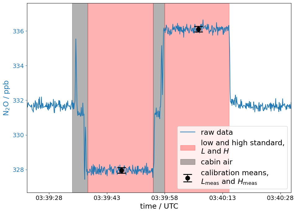
Figure 2 Example of an in-flight two-point calibration from the ASIA-AQ campaign. When a calibration sequence is activated first an internal valve of the MGA³ switches from the sample air inlet to the calibration gas inlet. Then, during the first time span (gray area), cabin air is drawn in via the overflow of the calibration system. Shortly after the solenoid valve for the low standard calibration gas L is activated for about 20 s allowing the gas to be drawn in by the MGA³ (first red area). Then the solenoid valve closes and cabin air is shortly drawn again (second gray area) until the second solenoid valve activates for the high standard calibration gas H (second red area). In total the calibration process lasts for about 40 s. The black dots are the mean values L_meas and H_meas of L and H with their respective errors, which are then used for the calibration to relate to the known reference values of the calibration gases.

Table 2 Mole fraction values of each high and low standard gas pair for the GHGMon and ASIA-AQ campaign.

To calculate the calibrated time series ${{\mathrm{N}}_{\mathrm{2}}\mathrm{O}}_{\mathrm{cal}}\left(t\right)$ out of a measured raw data time series ${{\mathrm{N}}_{\mathrm{2}}\mathrm{O}}_{\mathrm{raw}}\left(t\right)$ that is provided by the MGA³, we first calculate a scale factor m_n and an offset d_n for each calibration cycle n=1, …, N for all N∈ℕ cycles, according to Pitt et al. (2016) with:

$$\begin{array}{}\text{(1)}& m_n={\displaystyle \frac{H_{\mathrm{true}}-L_{\mathrm{true}}}{H_{\mathrm{meas},n}-L_{\mathrm{meas},n}}},n=\mathrm{1},\mathrm{\dots },N;N\in \mathbb{N}\end{array}$$

$$\begin{array}{}\text{(2)}& d_n=H_{\mathrm{true}}-m_n\cdot H_{\mathrm{meas}}.\end{array}$$

Here H_meas,n and L_meas,n are the means of the measured values for the high and low standards H and L as shown for one calibration cycle n in Fig. 2. H_true and L_true represent their known true mole fractions in Table 2. We interpolate the scale factors m_n and offsets d_n between every calibration cycle for every time point t in the measured time series ${{\mathrm{N}}_{\mathrm{2}}\mathrm{O}}_{\mathrm{raw}}\left(t\right)$ and get the continuous scale factor m(t) and offset d(t) which lead us to the calibrated values ${{\mathrm{N}}_{\mathrm{2}}\mathrm{O}}_{\mathrm{cal}}\left(t\right)$:

$$\begin{array}{}\text{(3)}& {{\mathrm{N}}_{\mathrm{2}}\mathrm{O}}_{\mathrm{cal}}\left(t\right)=m\left(t\right)\cdot {{\mathrm{N}}_{\mathrm{2}}\mathrm{O}}_{\mathrm{raw}}\left(t\right)+d\left(t\right).\end{array}$$

For our H₂O measurements, we only use a zeroing procedure, since both L and H standards are dry and should not contain any H₂O. Here, we calculate the difference d_n between the mean V_meas,n of a measured calibration cycle of only one of the two cylinders and its assumed actual value V_true=0. We obtain the calibrated value ${{\mathrm{H}}_{\mathrm{2}}\mathrm{O}}_{\mathrm{cal}}\left(t\right)$ by interpolating d_n for every t to d(t):

$$\begin{array}{}\text{(4)}& {\displaystyle }{d}_n=V_{\mathrm{true}}-V_{\mathrm{meas},n},n=\mathrm{1},\mathrm{\dots },N;N\in \mathbb{N}\text{(5)}& {\displaystyle }{{\mathrm{H}}_{\mathrm{2}}\mathrm{O}}_{\mathrm{cal}}\left(t\right)={{\mathrm{H}}_{\mathrm{2}}\mathrm{O}}_{\mathrm{raw}}\left(t\right)+d\left(t\right).\end{array}$$

For the uncertainty of our cylinders we use the standard error for every mean calculated from the L and H standards in the calibration cycles, resulting in uncertainties below 1 ppb. Experience from GHGMon showed that the respective differences between the standards of about 3 ppb in N₂O were too small causing issues while calibrating the data, especially with the error calculation for the calibration procedure. Based on this and the later experience from ASIA-AQ flights, we recommend that the differences between the high and low standards including the errors of the cylinder values should be at least two orders of magnitude higher than the precision of the MGA³.

2.4 MGA³ mole fraction retrieval software and versions

In this section, we explain how the MGA³ software retrieves the mole fraction values C from its measurements. The lasers of the MGA³ emit light in a wavenumber range close to the absorption lines of the target species such as N₂O. The laser beam is directed into the measurement cell where the target sample air is located. There, the intensity I₀ of the laser beam weakens through absorption by the sample air. After the laser beam exits the cell, it illuminates a detector which measures the intensity I along the wavelengths, i.e. the absorption spectrum and therefore the absorption line profile of the N₂O. Each measured spectrum is then provided as the transmittance τ(ν) by the MGA³. The measured absorption line profile can either be fitted online while measuring or later on at any time with the MGA-ReFit software. The lines are fitted by minimizing the sum of least-squares using the Beer-Lambert law, which in this case is based on a Voigt profile:

$$\begin{array}{}\text{(6)}& \mathit{\tau }\left(\mathit{\nu }\right)={\displaystyle \frac{I\left(\mathit{\nu }\right)}{I_{\mathrm{0}}\left(\mathit{\nu }\right)}}=\exp \left(-\mathit{\alpha }(\mathit{\nu },p,T)\cdot N_{\mathrm{0}}(p,T)\cdot L\cdot C\right).\end{array}$$

Here N₀ is the Loschmidt constant and ν represents the wavenumber. By knowing the pressure p, the temperature T and the optical path length L of the measurement cell, the software can calculate the absorption coefficient α and the mole fraction C of the measured species (Hundt et al., 2018). The absorption coefficient α represents the shape of the Voigt profile for a specific molecule including the Half-Width-Half-Maximum (HWHM) of its absorption line profile if only one such molecule is observed (see Appendix A). The mole fraction C then scales α for more than one molecule.

In this paper we use two different versions of the MGA³ fitting software. The original software of our MGA³ model, which we denote as version 1 (v1) (V30.0.171.0), does not correct for water vapor dependencies. That means that it fits each measured absorption line applying Eq. (6) and calculates the mole fraction C, but does not account for dilution and it cannot account sufficiently enough for all quantum-mechanical effects, such as water vapor line broadening, on the data, since not all processes are known or can be determined. To correct for these water vapor dependencies we conducted a water vapor experiment in the laboratory which we use to determine an empirical water vapor correction as shown in Sect. 3. This correction is then applied during the data post-processing to the already retrieved C time series. In parallel, an updated version of the fitting software was developed by MIRO Analytical. The new version is based on the same laboratory experiment and now includes a correction for water vapor dilution and broadening effects already implemented in the fitting process of the spectra. The software version (V30.1.59.0) is in the following referred to as version 2 (v2). The resulting v2 time series of the retrieved mole fractions C does not longer require the postfit corrections as in v1.

2.5 Fitting with constant HWHM – the β option

For the software version v1, the MGA³ has the option to activate or deactivate the β, which is, within the MIRO software, an internal measure for the HWHM of each absorption line and therefore for the absorption coefficient α (see Appendix A). If the β is deactivated, the MGA³ freezes the HWHM of the respective absorption line for all upcoming spectra and uses the last used value when the β was still active. This means, however, that consequently the mole fraction C in the fitting function (6) has to account for any changes that would occur in α. This leads to deviations from the actual values in C. However, with high water vapor contents in the sample air, as we show in Appendix A, the HWHM solely depends on water vapor for our N₂O spectral line. Based on this, the mole fraction C time series with a frozen β can subsequently be corrected by an empirical water vapor correction. In the following, we denote this water vapor corrected data as v1-β-off. To enforce the same behavior for all v1-β-off refit-processes as much as possible, we deactivate the β always when dry gas is measured and therefore no water vapor should be present.

At this point, the mole fractions retrieved by v1-β-off should not differ compared to water vapor corrected data retrieved with v1 and an activated β – from here on denoted as v1-β-on. However, due to the α being kept constant in v1-β-off the fitting software has one parameter less to account for in the fitting process which results in less numerical noise in C compared to v1-β-on. Software version v2 does not have a β option and already corrects for water, and therefore will be simply denoted as v2. These correction approaches will now be discussed in more detail in Sect. 3.

3 Water vapor correction approaches of N₂O in this study

Water vapor is highly variable in the atmosphere with 1–10 ppm in the Upper Troposphere – Lower Stratosphere (UTLS) (Kaufmann et al., 2016) and even up to 30 000 ppm within the tropical boundary layer as shown in Fig. 5 from the ASIA-AQ measurements. Due to this high variability of water vapor in different regions of the world and its volatility, GHG measurements are usually reported in dry mole fractions for better comparability, which requires precise water vapor measurements at all times (Chen et al., 2010; Rella et al., 2013). The first step is to eliminate the dilution from the gas due to the present H₂O by using the following equation:

$$\begin{array}{}\text{(7)}& C_{\mathrm{dry}}={\displaystyle \frac{C_{\mathrm{wet}}}{\mathrm{1}-C_{{\mathrm{H}}_{\mathrm{2}}\mathrm{O},\mathrm{abs}}}}.\end{array}$$

Here, C_wet denotes the mole fraction of N₂O diluted by H₂O. $C_{{\mathrm{H}}_{\mathrm{2}}\mathrm{O},\mathrm{abs}}$ is the absolute mole fraction of the H₂O not influenced by any spectroscopical effects distorting the the measurements. C_dry represents the mole fraction of N₂O in the gas mixture after the removal of H₂O. However, additional spectroscopic effects, such as water vapor line broadening, or instrument-specific behaviors in the measurements can have an impact on the data if not accounted for correctly or not at all. Those effects then often have to be corrected by using an empirical water vapor correction, also specific to each instrument (e.g. Chen et al., 2010; Rella et al., 2013; Pitt et al., 2016; Gvakharia et al., 2018).

Since the original MGA³ software v1 does not provide a water vapor correction, neither for dilution nor completely for spectroscopic effects, we first derive an empirical water vapor correction from a laboratory experiment, further described in Sect. 3.1. With the parameters a₀ and b₀ determined from a quadratic function in the laboratory, we apply the following water vapor correction equation also used by Rella et al. (2013) to account for all potential H₂O dependencies:

$$\begin{array}{}\text{(8)}& C_{\mathrm{dry}}={\displaystyle \frac{C_{\mathrm{wet}}}{a_{\mathrm{0}}\cdot C_{{\mathrm{H}}_{\mathrm{2}}\mathrm{O}}^{\mathrm{2}}+b_{\mathrm{0}}\cdot C_{{\mathrm{H}}_{\mathrm{2}}\mathrm{O}}+\mathrm{1}}},\end{array}$$

which we will explain more thoroughly in Sect. 3.2. Here $C_{{\mathrm{H}}_{\mathrm{2}}\mathrm{O}}$ is the mole fraction of H₂O as measured by the instrument possibly including the influence spectroscopical and dilution effects. In the following, we shortly introduce how we attain four water vapor corrected mole fraction data sets, retrieved from a single measured spectral data set, by different approaches.

v1-β-on

The wet mole fractions C_wet for N₂O and $C_{{\mathrm{H}}_{\mathrm{2}}\mathrm{O}}$ for H₂O are retrieved by the software version v1 and with an activated β. The time series C_wet is then water vapor corrected to obtain C_dry by using Eq. (8). The data for the lab experiment from which we derive our correction is also fitted with the software version v1 with an active β (see Sect. 3.1).

v1-β-off

This approach is identical to v1-β-on except that the β is deactivated during all fitting and retrieval processes by the MGA³ software.

v1-β-off-DLH

A precise water vapor correction approach requires precise water vapor measurements. Hence, for this specific approach, we first retrieve the wet mole fractions C_wet for N₂O and $C_{{\mathrm{H}}_{\mathrm{2}}\mathrm{O}}$ for H₂O with a deactivated β, as for v1-β-off, and then compare our MGA³-H₂O measurements to the H₂O measurements made by NASA's well established Diode-Laser-Hygrometer (DLH) at the ASIA-AQ campaign (Diskin et al., 2002). Thereby, we checked the stability of the MGA³ water vapor measurements over multiple flights and adjusted the MGA³-H₂O measurements accordingly to the DLH-H₂O measurements to achieve the same standard for the MGA³-H₂O measurements over all the flights (see Sect. 3.3 for more details). The mean behavior of the MGA³-H₂O measurements of all flights compared to the DLH-H₂O measurements is also used to calibrate the the MGA³-H₂O measurements from the laboratory experiment from which the water vapor correction is derived. Then the DLH-adjusted $C_{{\mathrm{H}}_{\mathrm{2}}\mathrm{O}}$ and the DLH-adjusted correction function from the laboratory experiment are used for correcting C_wet to C_dry using the correction function (8).

v2

In this approach, we use the newly implemented MGA³ retrieval software v2 which already includes a water vapor correction based on the same laboratory experiment as used for the previous approaches. The water vapor correction, however, is applied already while fitting the spectra and not after the N₂O mole fraction C_wet is retrieved. Here, the H₂O spectra are directly used to correct the N₂O spectra and directly report corrected C_dry mole fractions. The H₂O spectra or measurements are not adjusted to the DLH measurements beforehand as for v1-β-off-DLH.

3.1 Laboratory Experiment

In this section, we explain the setup of the laboratory experiment for the water vapor correction, how we conducted it and how we prepared the data retrieved from this experiment for the water vapor correction equation. For the laboratory experiment, we change the calibration system in Fig. 1 from the “in-flight calibration” configuration to the “laboratory humidifying” configuration in Fig. 3 and only use the calibration gas inlet of the MGA³ throughout the whole experiment. The sample gas is provided by a gas cylinder (cal gas 1) and is first divided into two sub-lines, which are controlled by a mass flow controller each. One sub-line (line 1) is provided with only 3 slpm by its mass flow controller (MFC 1), since the humidifier (Dew Point Generator LI-610, LICOR) only operates with mass flows up to 2.5 slpm. The excess gas in line 1 is then released through the overflow behind the MFC 1 to protect the humidifier. The output of the humidifier is controlled in a range of 0–2.5 slpm with a valve on the humidifier itself. The second sub-line (line 2) is provided with 0–5 slpm by the MFC 2 which directly merges with the humidified output from line 1. The length of the mixing line is 1.5 m to allow for optimal mixing of dry gas and humidified gas. The merged gas then directly flowes into the MGA³, which is set to operate with a mass flow of 1.9 slpm for this experiment. The excess gas in the mixing line is released through an overflow in front of the MGA³. The second gas, cal gas 2, is used only for calibration purposes. The settings are the same as in the airborne setup at the GHGMon and the ASIA-AQ campaigns (see Sect. 2.2) with a cell pressure of  70 hPa and a cell temperature T of 25 °C.

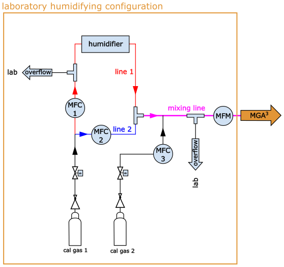
Figure 3 Scheme of the setup of the water vapor laboratory experiment. To fully function the orange box gets exchanged with the orange box of the in-flight calibration configuration in Fig. 1.

For the experiment, the MFC 2 is first set to 5 slpm and the humidifier output to 0 slpm, allowing only for the dry gas from cylinder 1 to be sampled. Then, the output of the humidifier is increased stepwise from 0 to 2.5 slpm, increasing the mole fraction of water vapor in the mixing line. Once the maximum mass flow for the humidifier output is reached, the mass flow of MFC 2 is incrementally decreased from 5 to 0 slpm, further increasing the humidity in the merged gas until only the output from the humidifier is sampled. Thereby, a range of water vapor mole fractions of 0 %–3 % is covered. This process of humidifying is repeated four times. Before and after each repetition, the gas from cylinder 2 is sampled for calibration purposes.

The recorded spectral data are then refitted with three different water correction approaches. Twice with the original software version v1 (once with an activated β and once with a deactivated β) and once with the updated version v2. Figure 4 shows the retrieved N₂O mole fractions from all those three approaches versus the retrieved H₂O mole fractions after calibrating the time series to the dry cylinder gases. As obvious from Fig. 4a and b for v1, the uncorrected N₂O (blue dots) mole fraction varies by more than 10–18 ppb in humid versus dry conditions. The cyan line gives the expected impact of the dilution effect only compared to dry conditions. The measured raw data deviate from the expected behavior due to spectroscopic effects like pressure broadening, which not all can be accounted for by the software in general. Also the pressure self broadening of H₂O can be a cause of deviation in the measurements (Rella et al., 2013) if not corrected for. Furthermore, we only use zero measurements to calibrate the H₂O, which could be a reason for the deviations from the cyan line. Since we use dry calibration gas in both cylinders, we cannot account for changes in sensitivity of the H₂O measurements for values above 0. With the deactivated, frozen β in v1 the deviation is larger than with the activated β since the water vapor line broadening is not accounted for in this setting (see Sect. 2.5). Figure 4c shows the mole fractions retrieved with the updated software version v2, in which the N₂O mole fractions are already corrected for water vapor during the fitting process of the measured spectra (grey dots). For the raw data in Fig. 4a and b we first have to derive a correction which leads us to the corrected data sets v1-β-on and v1-β-off (grey dots). This, we show in Sect. 3.2.

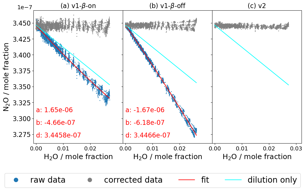
Figure 4 In panels (a) and (b) we can see the behavior of the raw N₂O with increasing H₂O mole fractions (blue dots) during laboratory water vapor experiment for v1-β-on and v1-β-off. The red lines are fitting functions giving us the parameters for our water vapor correction function in Sect. 3.2. The cyan line shows the expected behavior of the raw mole fractions if only dilution was having an effect on the measurements. The grey dots are the blue dots corrected by the water vapor correction function (17) in Sect. 3.2. In panel (c) the grey dots represent the raw mole fraction output of the experiment when reprocessed with version v2 of the MGA-ReFit software. The data were are already corrected for water vapor influences based on the same data in panels (a) and (b) while they were being reprocessed.

3.2 Water Correction Function

In the next step, we correct the raw N₂O data in Fig. 4a and b and derive a water vapor correction function. For this, the wet raw data C_lab,wet given in Fig. 4a and b are fitted with a quadratic function (red line), giving us the parameters a, b, d:

$$\begin{array}{}\text{(9)}& \mathrm{fit}\left(C_{{\mathrm{H}}_{\mathrm{2}}\mathrm{O}}\right)=a\cdot C_{{\mathrm{H}}_{\mathrm{2}}\mathrm{O}}^{\mathrm{2}}+b\cdot C_{{\mathrm{H}}_{\mathrm{2}}\mathrm{O}}+d.\end{array}$$

Here, $C_{{\mathrm{H}}_{\mathrm{2}}\mathrm{O}}$ is the H₂O mole fraction. In an ideal fit, the parameter d represents the actual value of the dry cylinder mole fraction for $C_{{\mathrm{H}}_{\mathrm{2}}\mathrm{O}}=\mathrm{0}$ and therefore simultaneously the dry target value after the water vapor correction is applied for all $C_{{\mathrm{H}}_{\mathrm{2}}\mathrm{O}}$. To obtain the water vapor corrected mole fraction $C_{\mathrm{lab},\mathrm{dry}}=d$ for N₂O in this laboratory experiment, the value of the correction function (9) is subtracted without the parameter d from C_lab,wet:

$$\begin{array}{}\text{(10)}& C_{\mathrm{lab},\mathrm{dry}}=C_{\mathrm{lab},\mathrm{wet}}-(a\cdot C_{{\mathrm{H}}_{\mathrm{2}}\mathrm{O}}^{\mathrm{2}}+b\cdot C_{{\mathrm{H}}_{\mathrm{2}}\mathrm{O}}).\end{array}$$

However, the parameters of this fit function apply only for the specific mole fraction d of the used cylinder and not necessarily for cylinders with random mole fractions C_dry. If a humidified air sample containing no N₂O were sampled, these specifically determined parameters would still produce a correction value for the corresponding $C_{{\mathrm{H}}_{\mathrm{2}}\mathrm{O}}$, despite the absence of the N₂O. To account for any other values C_dry in the cylinder, we use following boundary condition:

$$\begin{array}{}\text{(11)}& {\displaystyle }{C}_{\mathrm{dry}}=\mathrm{0}\iff {\mathrm{fit}}_x\left(C_{{\mathrm{H}}_{\mathrm{2}}\mathrm{O}}\right)=\mathrm{0}\forall C_{{\mathrm{H}}_{\mathrm{2}}\mathrm{O}}>\mathrm{0}\text{(12)}& {\displaystyle }\Rightarrow a,b,d=\mathrm{0}\end{array}$$

and assume that the parameters a, b and c – consequently the fit Eq. (9) – approach 0 proportionally with decreasing mole fractions C_dry, giving:

$$\begin{array}{}\text{(13)}& {\displaystyle }a={\displaystyle \frac{a-\mathrm{0}}{d-\mathrm{0}}}\cdot C_{\mathrm{dry}}={\displaystyle \frac{a}{d}}\cdot C_{\mathrm{dry}}=a_{\mathrm{0}}\cdot C_{\mathrm{dry}},\text{(14)}& {\displaystyle }b={\displaystyle \frac{b}{d}}\cdot C_{\mathrm{dry}}=b_{\mathrm{0}}\cdot C_{\mathrm{dry}},\text{(15)}& {\displaystyle }d={\displaystyle \frac{d}{d}}\cdot C_{\mathrm{dry}}=d_{\mathrm{0}}\cdot C_{\mathrm{dry}}=C_{\mathrm{dry}},\text{(16)}& {\displaystyle }{C}_{\mathrm{dry}}=C_{\mathrm{wet}}-\left(a_{\mathrm{0}}\cdot C_{\mathrm{dry}}\cdot C_{{\mathrm{H}}_{\mathrm{2}}\mathrm{O}}^{\mathrm{2}}+b_{\mathrm{0}}\cdot C_{\mathrm{dry}}\cdot C_{{\mathrm{H}}_{\mathrm{2}}\mathrm{O}}\right).\end{array}$$

C_wet is the measured wet mole fraction of N₂O using the new cylinder with C_dry. The fit parameters in Eqs. (13)–(15) are now dependent on the mole fractions C_dry in the cylinder and from Eq. (16) we get:

$$\begin{array}{}\text{(17)}& C_{\mathrm{dry}}={\displaystyle \frac{C_{\mathrm{wet}}}{a_{\mathrm{0}}\cdot C_{{\mathrm{H}}_{\mathrm{2}}\mathrm{O}}^{\mathrm{2}}+b_{\mathrm{0}}\cdot C_{{\mathrm{H}}_{\mathrm{2}}\mathrm{O}}+\mathrm{1}}},\end{array}$$

which can finally be used for any random measurement C_wet with a simultaneously measured $C_{{\mathrm{H}}_{\mathrm{2}}\mathrm{O}}$. Equation (17) is the same as the one used by Chen et al. (2010) and Rella et al. (2013), also with the assumption that the water vapor correction is proportional to the mole fraction of our observed species.

The correction Eq. (17) is then applied to the raw data in Fig. 4a and b and results in the grey corrected data v1-β-on and v1-β-off. With this, our retrieved data is corrected for water vapor and influences and should be independent of water vapor changes either by dilution or spectral effects like line broadening. The main difference between the β-on and β-off retrieved data is that the noise in the data for the β-off data is smaller (see Sect. 2.5) by roughly 42 % compared to its respective β-on retrieved data, which will be discussed in Sect. 3.5 in more detail.

3.3 H₂O calibration against DLH absolute ambient measurements

The quality of the water vapor measurement is decisive for a precise water vapor correction. While the absolute accuracy is not of main importance, the stability of the water vapor measurement is, hence, the replicability of the H₂O measurements over time. To analyze the stability of the MGA³-H₂O measurements in our setup, we compare data from 14 flights from the ASIA-AQ campaign with absolute ambient H₂O vapor measurements measured by the established DLH. We use the DLH because it reliably reports stable water vapor measurements which can be used to effectively correct the MGA³ water vapor measurements. In our airborne measurement setup the MGA³-H₂O is only zeroed with our dry cylinder gases, leading to differences in the data between the two instruments. Also the self broadening of H₂O can lead to differences as discussed in Sect. 3.1. In Fig. 5a the DLH-H₂O for each of the 14 flights is plotted against the respective MGA³-H₂O data for the β-off setting. The flights were conducted over a time span of roughly two months. The lines are polynomial fits (second order) of the measurements, calculated by applying orthogonal distance regressions. The dashed red line shows a slope of 1. The dashed black line shows the mean of all curves which in this case is a orthogonal distance regression fit to the data of all the lines and which is also a quadratic function described with $f\left(x\right)=a{x}^{\mathrm{2}}+bx+d$. The difference in the length of every curve is due to the differences in the maximum measured humidity during each flight.

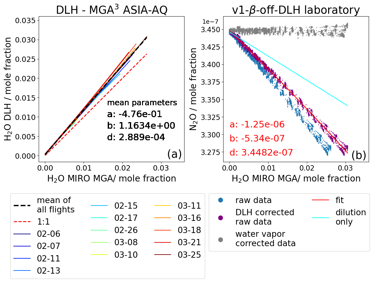
Figure 5 In panel (a) we plotted the DLH-H₂O measurements against the MGA³-H₂O measurements for the mole fractions retrieved with v1 with a deactivated β for 14 ASIA-AQ flights from 6 February to 25 March. In general, our instrumental setup measured less H₂O than DLH. With increasing H₂O the MGA³ measurements seem to deviate more from each other indicating changes in sensitivity of the instrument. The black dashed line shows the mean for all flights which is a orthogonal distance regression fit through all the data of the lines. Panel (b) shows again the same as Fig. 4b but now the blue raw data is first corrected by the respective dashed black line in panel (b) resulting in the “DLH-corrected” purple dots. The red lines are now the fitting lines for the purple data, which parameters now can be used to derive the new correction v1-β-off-DLH.

In general, the DLH measures about b=1.16 times higher H₂O values than the MGA³ with our instrumental setup, which is mainly due to not being able to conduct a two-point-calibration as mentioned. Other minor reasons could be, for example, water vapor tube dampening effects through the long 6.5 m PTFE inlet tubing in our setup. At the instrument flow rate of approx. 13 slpm, it takes about 2 s at 1 atm until the sample air reaches the measuring cell, during which water vapor could attach and slowly unstick from the inner tubing walls. Still, the results show that H₂O measurements for the flights diverge for higher H₂O values, indicating changes in the sensitivity. In principle, this can only be accounted for by a sufficient two-point-calibration as explained in Sect. 3.1. The changing behavior over the flights, however, means that the once attained correction equation in the laboratory will behave slightly differently for every flight unless the MGA³-H₂O is standardized to a norm.

To account for this variability in behavior of the MGA³-H₂O from flight to flight, we constructed a new correction specifically for all the ASIA-AQ flights in addition to the already existing v1-β-off approach in Sect. 3.2, called v1-β-off-DLH, which can be seen in Fig. 5b (grey dots). First, since the H₂O measurement in the laboratory water vapor experiment cannot be calibrated against absolute reference values – due to our used humidifying configuration setup not being able to provide such an accurate value – we assume that the H₂O behavior in the experiment is similar to the mean behavior of all flights (dashed black line in Fig. 5a). Thus, we correct our laboratory experiment H₂O values with this mean (see Sect. 3.4 for explanation). This results in the purple DLH corrected data in Fig. 5b. We can see that the DLH adjusted N₂O raw data is closer to the cyan line which represents the ideal behavior if only dilution existed. Now, the fit (red line) is used for deriving the parameters of our water vapor correction in the same way as for v1-β-off. However, before the correction function is applied to the flight data, we first correct the H₂O flight measurements with their respective line in Fig. 5a to assure that all flight measurements and the laboratory H₂O measurements are “calibrated” to the same standard, which in this case are the DLH measurements. Now, the water vapor correction function can be applied to the flight data giving the water vapor corrected mole fraction data. This approach is denoted as v1-β-off-DLH.

In the next section, we compare the results from the different correction approaches v1-β-off, v1-β-off-DLH and v2.

3.4 Comparison of the different water correction approaches

In this chapter, we compare the data retrieved by the different MGA³ software versions and water correction approaches v1-β-off, v1-β-off-DLH and v2 with the data measured by NASA's established DACOM spectrometer. The DACOM is a TDLAS designed for CO measurements but it also measures CH₄ and N₂O. It has a temporal resolution of 5 Hz and dries the sample air via a Nafion tube before sampling, negating water vapor interference and dilution effects. Our calibration cylinders for the MGA³ were cross calibrated against the NOAA calibration cylinders of DACOM. This makes the DACOM measurements ideal for the validation of our water vapor correction approaches for the MGA³-N₂O measurements. For a better comparison, the MGA³ data was resampled to 5 Hz to match the DACOM data. We chose to compare three flights in Thailand for which data from both instruments are available, well calibrated and, most importantly, high H₂O variability was measured.

Figure 6a, b and c illustrate the difference between the DACOM-N₂O data and the MGA³-N₂O for three selected ASIA-AQ flights (25, 21 and 18 March 2024). Different colors represent data retrieved using the different MGA³ approaches (v1-β-off in orange, v1-β-off-DLH in green and v2 in black). The lines represent the mean values for 0.01 % (100 ppm) H₂O bins. The blue shaded areas show the combined uncertainties of the DACOM measurements and the v1-β-off-DLH data. However, for the combined uncertainties, we do not use the 0.01 % H₂O bins resolution, but uncertainties of the full 5 Hz resolution to capture the variability of the instruments more accurately. Since our MGA³ calibration cylinders were calibrated against the DACOM NOAA cylinders, the accuracy determined from the uncertainty in the NOAA cylinders should have the same effect on the accuracy of our calibration cylinders. Therefore, for the combined uncertainty we only include the precision of DACOM and the total uncertainty of the MGA³, which includes the precision of each data point and the uncertainty of the cross calibration procedure. The uncertainties we used are always 1σ uncertainties.

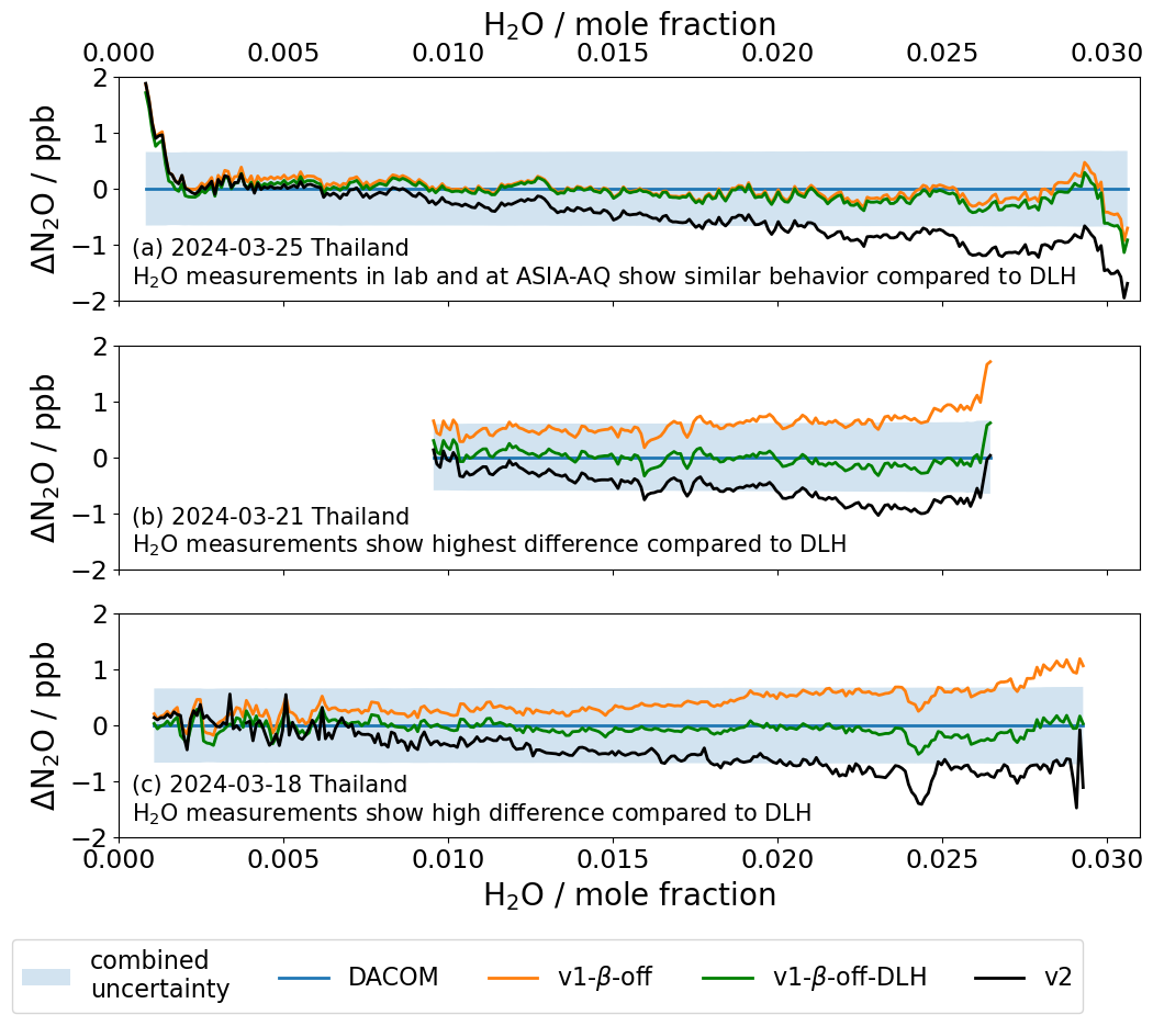
Figure 6 Differences between N₂O data measured by DACOM and the MGA³ for the different water vapor correction approaches v1-β-off, v1-β-off-DLH and v2 for three ASIA-AQ flights on the 25 March 2024 (a), 21 March 2024 (b) and 18 March 2024 (c). The colored lines show the mean values of the differences between DACOM and the MGA³ corrected data in 0.01 % or 100 ppm H₂O bins. The shaded blue areas represent the combined uncertainties of DACOM and the MGA³ with v1-β-off-DLH but at full resolution and not with the 0.01 % bin resolution.

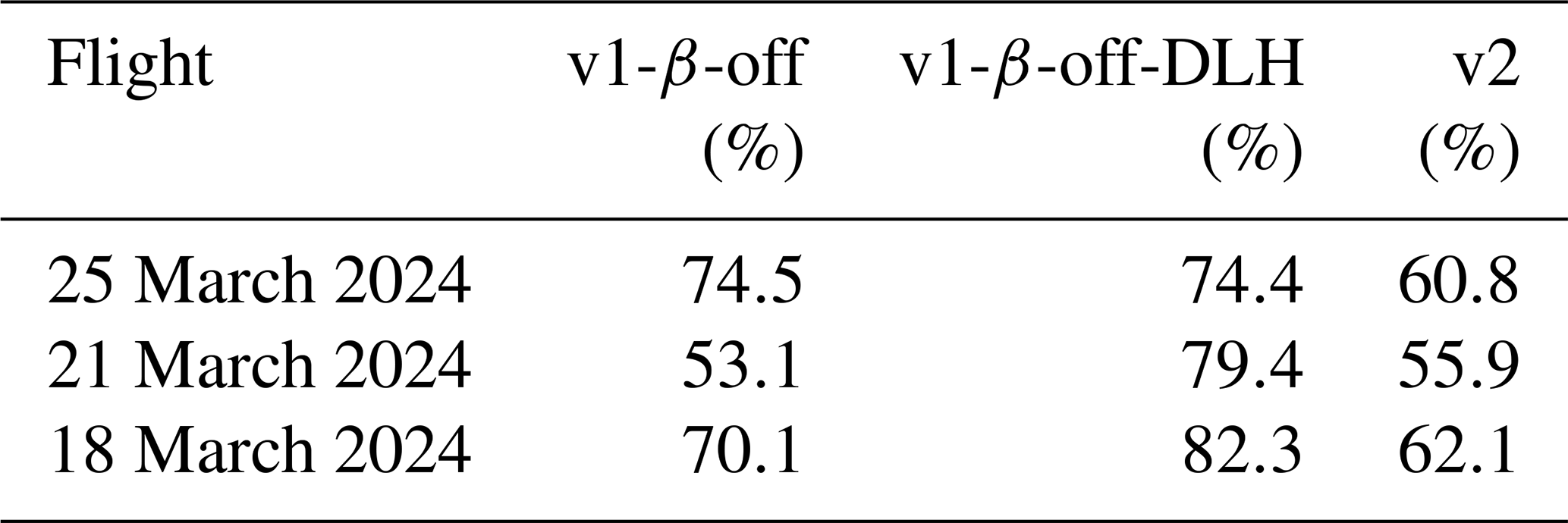
To quantify the agreement between the MGA³ measurements and DACOM, we calculate the fraction of data points that overlap within the combined uncertainty of both instruments which is summarized in Table 3. In Fig. 6a for the 25 March 2024, the difference between DACOM and v1-β-off (orange line) is already very small with 74.5 % of data overlapping between the two instruments. This indicates that the behavior of H₂O of the water laboratory experiment is actually close to the mean behavior for all ASIA-AQ flights (dashed black line, Fig. 5) and therefore to the behavior during this flight. This is indicated by the differences for v1-β-off-DLH (green line) which show only smaller deviations compared to v1-β-off due to the application of the DLH-correction (74.4 % overlap with DACOM). The differences for v2, however show a drift with increasing H₂O mole fractions with 60.8 % of data overlapping DACOM. In particular, for H₂O values above 1.5 % or 15 000 ppm the differences between DACOM and v2 are larger than the combined uncertainties. A reason for the drift can be unwanted behavior of the pressure regulator in our MGA³ which is influenced by different amounts of water vapor in the sampled air. In the newer models the regulator is replaced by a new kind of regulator which does not show such influences of water vapor (personal communication with Oleg Aseev). In Fig. 6b and c, the differences for v1-β-off show deviations greater than 1 ppb compared to DACOM. The overlap of the data is 53.1 % and 70.1 %, respectively. This can be explained by the indicated changes in the sensitivity of the MGA³-H₂O measurements as discussed in Sect. 3.3. When corrected with DLH, however, the resulting v1-β-off-DLH corrected data overlaps within 79.4 % and 82.3 % with DACOM data and the deviations for larger H₂O values decrease. For the 21 and 18 March 2024 in v2 the same trends are found in Fig. 6b and c as for the 25 March 2024 shown in Fig. 6a.

Table 3 Percentage of how many data points of the DACOM measurements overlap with MGA³ data with different water vapor correction approaches applied within the combined uncertainties at 5 Hz.

There are several possible reasons that the percentages of overlapping data with DACOM do not reach higher values than 82 %. First, of course, the two instruments are not identical and react inherently different to changes in the measured species especially due to the different setups (Nafion-dryer, inlet tubes, pump, mass flow, etc.). Here, the Nafion-dryer of the DACOM system and the inlet tubes of the MGA³ could have an influence on the respective sample air, resulting into differences in the measurements. Second, DACOM used one additional calibration cylinder and calibrates every 4 min while our setup uses only two cylinders for calibrations every 10 min, making our instrument potentially more prone to changes in sensitivity compared to DACOM. This issue can be overcome by using the same calibration method in the future. Third, it could be that the distance of the inlets for the two instruments of about 20 m leads to the sampled air by both instruments not being identical. In the case of v1-β-off-DLH, a last reason could be that the mean behavior of H₂O for all flights in Fig. 5a (dashed black line) correcting the laboratory experiment does not represent the actual true behavior. This could also explain the slight negative trend in N₂O from lower to higher H₂O values.

We conclude that the v1-β-off approach could be improved by the additional DLH correction resulting in the v1-β-off-DLH approach. The newer v2 version shows a significant drift for growing H₂O mole fractions but matches DACOM until 1.5 % or 15 000 ppm H₂O within the uncertainties. However, it does not need an additional adjustment with DLH data or data from other instruments as v1-β-off-DLH.

3.5 N₂O precision, noise and uncertainty

In Sect. 2.5, we explained the possibility of changing the β setting and how it influences the fitting process. An advantage from the deactivation of the β is, that the fitting software has one less parameter that has to be accounted for in the fitting process, leading to less noise in the retrieved mole fractions.

Therefore, we compare the precision of 14 ASIA-AQ flights refitted with the approaches v1-β-on, v1-β-off-DLH and v2. We determine the in-flight precision by calculating the mean of the precision values for each flight, obtained by propagating the standard deviations of all calibration time windows within the given flight, such as the one in Fig. 2. The mean N₂O precision for both the v1-β-off-DLH version and the v2 version is about 42 %±4 % lower than for the v1-β-on version. The best determined in-flight precision for a flight at ASIA-AQ with the v1-β-off-DLH version was approximately 0.17 ppb.

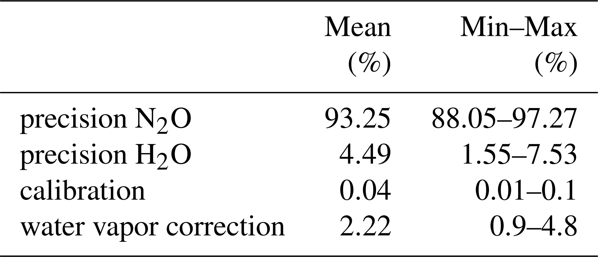
Further uncertainties arise from the calibration and the water vapor correction of the data. We summarize the uncertainty budget in Table 4 in percentages according to the contribution to the total uncertainty. After propagating the precision of the N₂O measurements through the calibration Eq. (3) and the water vapor correction Eq. (17) we find, that in the mean across flights the precision of N₂O contributes about 93 % to the squared total uncertainty. The H₂O-precision, usually in the range of approximately 0.01 vol %, contributes approximately 4.5 %, the calibration procedure about 0.05 % and the water vapor correction procedure about 2.2 % to the total squared uncertainty. However, in this calculation, we assume that the uncertainties of the NOAA-cylinders used for cross calibrating our own calibration cylinders are 0 and therefore only apply the uncertainties of our calibration cylinders which are <0.1 ppb using standard errors. The squared uncertainty of the H₂O measurements itself also increases by roughly 40 % after applying the DLH-correction to the ASIA-AQ data.

Table 4 Contribution of the N₂O-precision, H₂O-precision, calibration and water vapor correction procedure to the total squared uncertainty for the v1-β-off N₂O data in percentages.

The precision depends crucially on the optics alignment. Usually, we recognize a misalignment by a drop in the detected laser intensity, by worsened residuals when fitting the spectra or by worsened precision values compared to previous measurements which all can be corrected again by realigning the mirrors. The mirrors directing the laser beams into the measuring cell can misalign when the instrument experiences heavy shocks. We also experienced a misalignment after transporting the instrument with a van over several hours on the highway. Onboard the Cessna at the GHGMon campaign we did not experience any clear misalignment over the course of roughly 50 flight hours (including transfer flights). Onboard the DC-8 at ASIA-AQ, we did not experience any clear changes in the alignment either for about 90 flight hours. In South Korea, even after warming up the device for 1–3 h from temperatures slightly above the freezing point over night to 25 °C in the optics compartment of the instrument we could not see any significant changes to the alignment and precision. However, after the transfer flight from South Korea to Thailand, we experienced a clear misalignment in the optics worsening the precision of the instrument by about 50 %–100 % for the last four campaign flights. The optics could be realigned again in the laboratory after the campaign. The source of the misalignment could have multiple reasons, e.g, heavier shocks than usual while landing, but we could not identify any specific cause. In general, we realign the optics before every campaign for optimal data quality. Because of a possible misalignment, we recommend to built in the MGA³ in the top of a rack to have easier access to the mirrors while doing flight tests.

We conclude that the v1-β-off-DLH and v2 versions give a better precision for the data than the v1-β-on version. However, for the v1-β-off-DLH version to work, we have to determine an empirical water correction as described in Sect. 3 whereas version v2 works with no additional data refinement after the mole fraction retrieval. The instrument is stable in regards of its optical alignment over whole campaigns with about 50 flight hours and longer. Nonetheless, we recommend a realignment of the optics before every campaign for optimal data quality.

4 Stability of the DLR airborne MGA³ system

4.1 Allan Precision and calibration frequencies

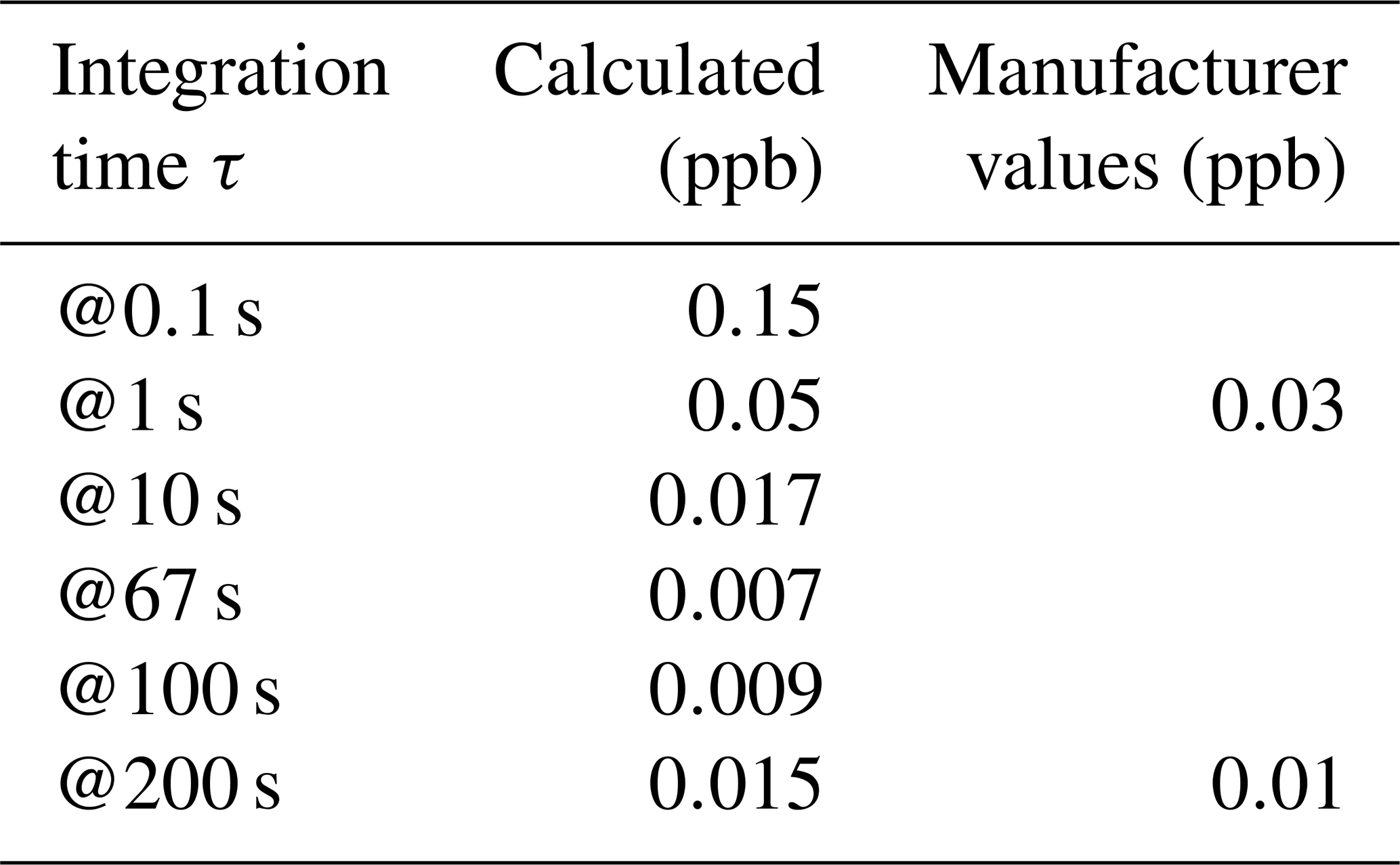
In this section, we determine the stability of the MGA³-N₂O via its Allan precision according to Werle et al. (1993), as can be seen in Fig. 7. We calculate the Allan precision from a 20 min time series of a measured calibration gas in the laboratory on ground and discuss the optimal calibration times and frequencies for the in-situ measurement. The range of white noise can be found along the orange line. The two green lines show the maximum and the minimum slope where the behavior of the instrument shows a drift. Based on this, the optimum integration time $\mathit{\tau }=\mathrm{67}\pm \mathrm{8}$ s was determined by calculating the mean of the times between the intersects of the green and orange lines. In Table 5, the result for a set of integration times τ can be seen, including two values that were given by the manufacturer. Our self-determined values are comparable to the manufacturer values but are slightly higher. Therefore, the data should be calibrated about every 67 s to avoid any drift in the data. However, this would lead to a duty cycle of about 63 % leading to a high and expensive calibration gas consumption. As a trade-off between data quality, gas consumption, and data acquisition, we chose to calibrate for 40 s in total every 10 min leading to a duty cycle of about 94 %, as we already saw in Fig. 2 in an example from the ASIA-AQ campaign. The calibration time windows show stable behavior within their respective 20 s and, in combination with the high cell exchange rate and after our experience at the GHGMon and ASIA-AQ campaigns, we suggest even shorter periods than 20 s for the high and low standards in future flights, further improving the duty cycle of our system. We have also calculated the Allan precision for in-flight data. In this case, however, we measured calibration gas for only 8 min due to limited availability of gas during the campaign. Also, the data was part of an cabin pressure experiment where we cannot distinguish the effects of cabin pressure change and the actual changes in stability, which we will show in Sect. 4.2.

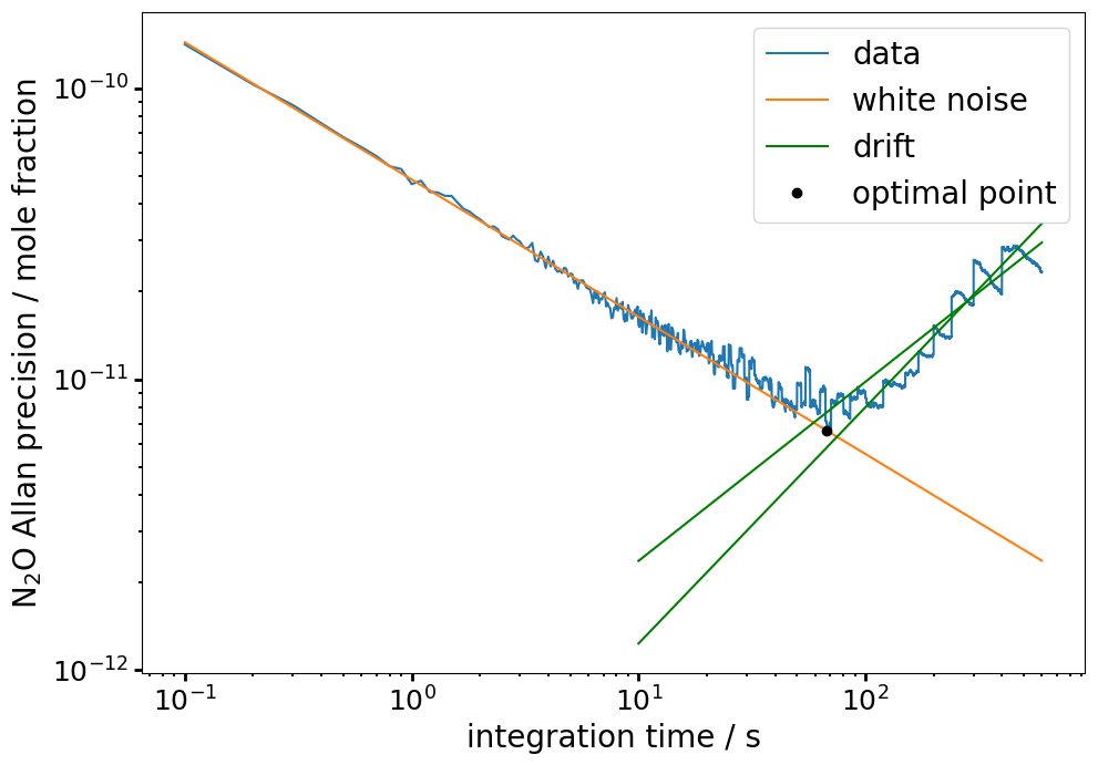
Figure 7 Allan Precision for N₂O. Values along the orange line are considered white noise. The green lines show the minimum and maximum range for drift behavior. The optimal integration time τ after which the drift sets in is shown with the black dot at $\mathit{\tau }=\mathrm{67}\pm \mathrm{8}$ s.

Table 5 Allan Precision for different integration times τ in Fig. 7. The optimal integration time is at 67 s. The values for τ=1, 200 s are slightly higher than the values given by the manufacturer.

4.2 Dependency on cabin pressure

As previously noted, the DC-8 aircraft has a pressurized cabin while the DLR Cessna aircraft is unpressurized. In the DC-8 the cabin pressure data are provided by the DC-8 Meteorological and Navigation Facility Instrumentation (MetNav). As a proxy for the cabin pressure in the Cessna, we use the static pressure measurement provided by the meteorological sensor package (METPOD). Previously, Pitt et al. (2016) have shown cabin pressure dependencies in their data resulting in deviations of several ppb for pressures ranging from about 1000 hPa down to 800 hPa, which were corrected by a pressure differentiated calibration procedure. However, with this procedure the data is filtered by a condition where the influence of pressure is small, leading to high losses in the amount of data. Gvakharia et al. (2018) also showed deviations in N₂O within a similar pressure range. These deviations were accounted for by frequent calibrations.

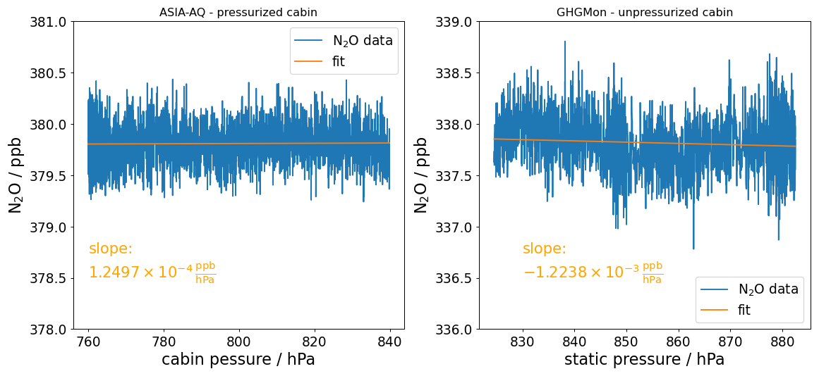
Figure 8 On the left, N₂O calibration gas measurements are plotted against the cabin pressure of the NASA DC-8. The pressure of the pressurized cabin was actively reduced from 840 to 760 hPa within 8 min. The slope of the fit function shows no significant drift in N₂O. On the right we see the N₂O calibration gas measurements plotted against the static pressure as a proxy for the cabin pressure, because the cabin of the DLR Cessna is not pressurized. During a descent within 8 min the static pressure increased from 820 to 880 hPa. The slope shows a significant drift for pressure changes of more than roughly 150 hPa, which would be higher than the precision of the instrument 0.17 ppb. However, the behavior seems to be less stable so that the drift does not seem to be connected to changes in cabin pressure alone.

To study the potential effect of cabin pressure on the measurement quality, we measured calibration gas during a specific descent of the DLR Cessna for about 8 min covering a pressure change from 820 to 880 hPa. To study the effect onboard the NASA DC-8, we specifically asked to actively lower the cabin pressure between 840 and 760 hPa within 8 min. Figure 8 shows the retrieved mole fractions of the sampled calibration gas, once plotted against the cabin pressure of the DC-8 and once against the static pressure for the DLR Cessna during the descent. For the ASIA-AQ data no obvious dependencies on the cabin pressure can be identified. The data seems to be stable, as can be seen from the fit of the data with a slope of $\mathrm{1.2497}\times {\mathrm{10}}^{-\mathrm{4}}$ ppb hPa⁻¹. For a pressure change in the range of 1000 hPa, the resulting drift would still almost be within the uncertainty/precision of 0.19 ppb of the instrument for these 8 min. However, for the GHGMon flight with the unpressurized cabin a less stable behavior with a standard deviation of 0.24 ppb can be seen, which is higher than the determined precision for this flight with 0.17 ppb. The fit function shows a slope of $-\mathrm{1.2238}\times {\mathrm{10}}^{-\mathrm{3}}$ ppb hPa⁻¹, but it does not show a clear linear behavior which would indicate a clear dependency on the cabin pressure alone. Another reason for the less stable behavior on the Cessna could be the different sizes of the aircraft. The Cessna is much smaller and is more prone to turbulences and vibrations in general. Especially during acceleration ascending this could have an effect on the data.

In Fig. 9 we also calculated the Allan precision for the cabin pressure experiment during ASIA-AQ in Fig. 8 on the left. We found the optimal point to be at about 13 s with an Allan precision of about 0.018 ppb and this point comes earlier than what we have determined in the ground measurements in Fig. 7. However, due to the limited availability of calibration gas during the campaign we were not able to perform a longer experiment for the determination of the stability of the instrument as we did in Fig. 7 on the ground. Therefore we cannot distinguish if the lower stability in-flight is due to the measurement in-flight itself or due to the cabin pressure changes.

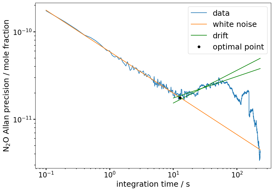
Figure 9 Allan precision of the cabin pressure experiment on the DC-8 at ASIA-AQ shown in Fig. 8 on the left. The optimal point is located at 12.8±0.9 s with an Allan precision of about 0.018 ppb, about 50 s earlier than calculated on the ground in Fig. 7. However, we cannot distinguish if the instrument is generally less stable in-flight or if this is only the case during cabin pressure change.

We conclude that the measurements from the unpressurized cabin are less stable but are probably not solely linked to cabin pressure changes alone. Nonetheless, we recommend for both a pressurized and unpressurized cabin to sample calibration gas before and after each relevant ascent or descent in a profile to minimize any drift.

4.3 Dependency on roll and pitch angle

In this section, we analyze if changes in the roll and pitch angle of the aircraft influence the measurements of the MGA³. For example, Pitt et al. (2016) introduced a quality flag for their data for roll angles over 10 °, which caused deviations in the measurements due to the centrifugal force acting on the alignments in the laser setup. The roll angle describes the rotation of the aircraft around its longitudinal axis (nose to tail) respective to its initial horizontal position of the wings (positive values: clockwise rotation looking forward) and the pitch angle describes the the rotation of the aircraft around its lateral axis (wing tip to wing tip) respective to its initial horizontal position (positive values: nose up). The roll and pitch angle data were provided by the DC-8 MetNav. The minium and maximum reached values for the roll angle during all flights at the ASIA-AQ campaign were $-\mathrm{36}\pm \mathrm{4}$ to 36±4 ° and for the pitch angle $-\mathrm{8}\pm \mathrm{2}$ to 15±2 °.

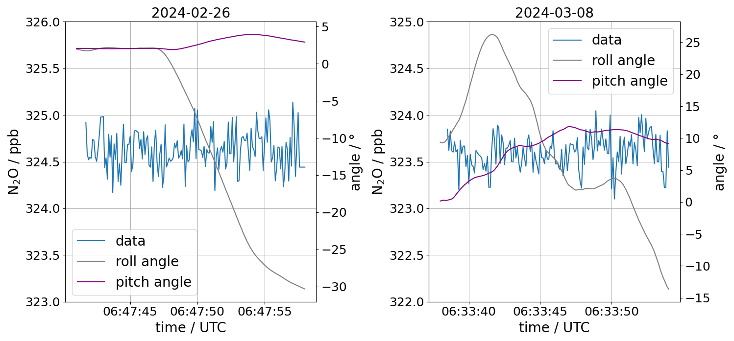
Figure 10 Calibration gas measured in-flight at the ASIA-AQ campaign during changing roll and pitch angles on 26 February and 8 March 2024 in South Korea. On 26 February 2024 we flew a left turn with a roll angle up to −30° while the pitch angle was almost constant. On 8 March 2024 we were ascending with a pitch angle of up to 12° while changing from a right turn to a left turn with roll angles from 25 to −15°. In both flights no dependencies that are larger than the respective noise of the measurements could be found.

In Fig. 10, we plotted data of 15 s from two calibration time windows from the flights on the 26 February and 8 March 2024 against the roll and the pitch angle of the aircraft. For both days we cannot see any clear dependency of the measurements on the angles that are larger than the noise or precision of our measurements. In Fig. 11, the left plot shows the standard deviation of N₂O calculated for each calibration time window of one calibration gas standard plotted against the pitch angle of the DC-8 during ASIA-AQ. The right plot shows the same, but for the roll angle. Each data point in the plot is calculated by roughly 12 s of data at 10 Hz. For Thailand we calculated a mean value of 0.39±0.05 ppb and for the Philippines and South Korea 0.18±0.3 ppb. In both cases no clear dependencies can be seen.

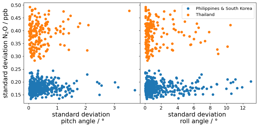
Figure 11 Standard deviation of N₂O for the calibration time windows of one calibration standard plotted against the standard deviation of the pitch angle (left) and the roll angle (right) at the ASIA-AQ campaign. Each data point in the plot is calculated by roughly 12 s of data. For both kinds of motion no clear dependency can be seen. The mean of the standard deviation values for Thailand is 0.39±0.05 ppb and for the Philippines and South Korea 0.18±0.3 ppb.

5 Case Studies and example measurements

In this section, we present calibrated and water vapor (v1-β-off-DLH) corrected N₂O measurements from the ASIA-AQ campaign. The goal of the campaign is to better understand the air quality in Southeast and East Asia through airborne in-situ measurements that later on can be used for validating models and satellite data (Crawford et al., 2025). The general approach was to fly the same pattern specifically designed for each country repeatedly for multiple flights to acquire data for large horizontal ranges within the PBL. The flight patterns were repeated two to three times per flight with frequent profiles to scan the whole PBL at different day times. Within a pattern, the profiles were flown at the same locations, as far as possible. With this, we acquired a N₂O data set with about 100 h of combined data measured at 10 Hz for the regions of Luzon (Northern Philippines), Taiwan, South Korea and Thailand in the winter of 2024. GPS-data and altitude above ground level (AGL) were provided or deduced from the measurements of the DC-8 MetNav. The wind measurements at flight altitude were provided in 20 Hz by the Meteorological Measurement System (MMS) (Scott et al., 1990) which is used on multiple NASA aircraft.

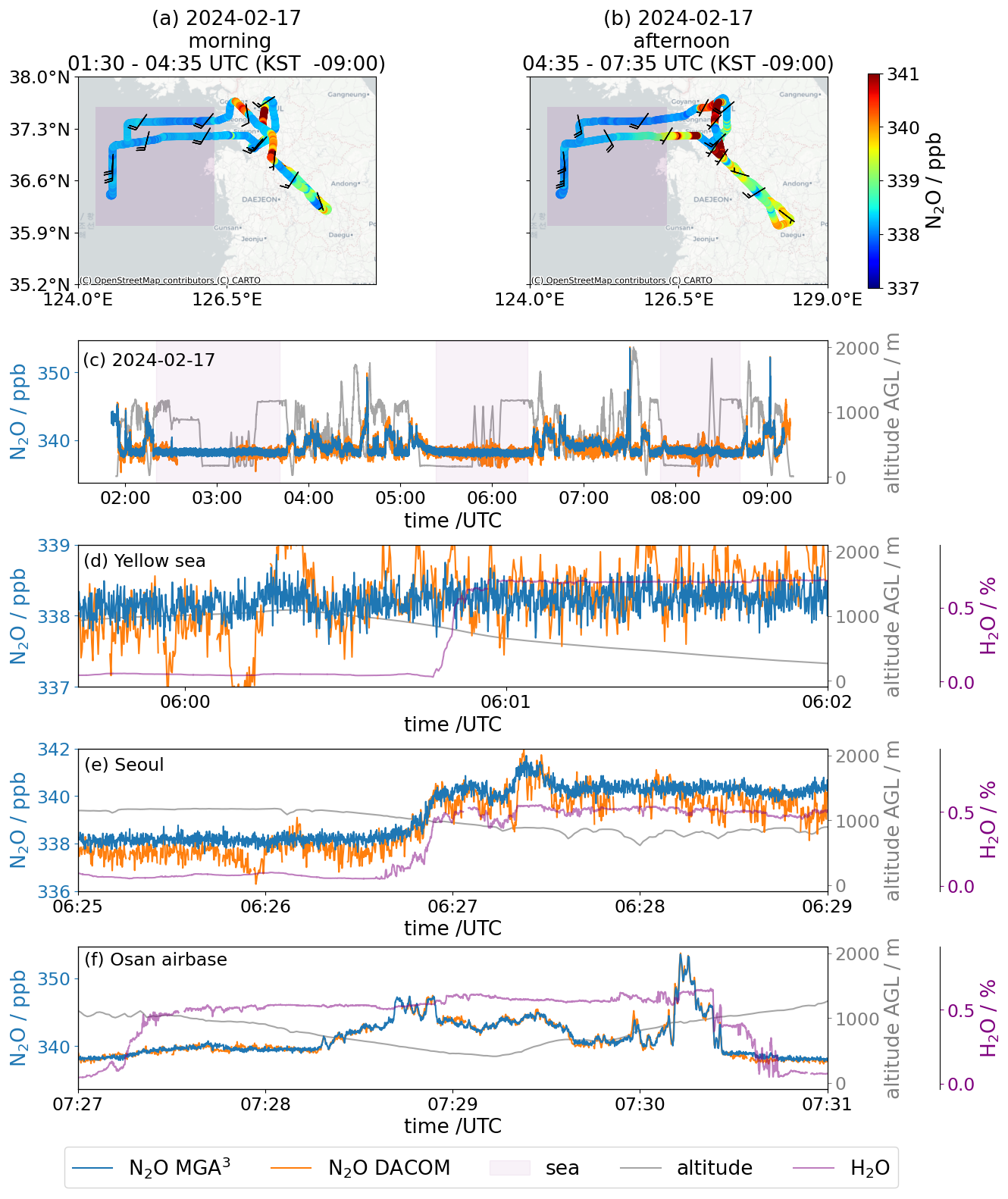
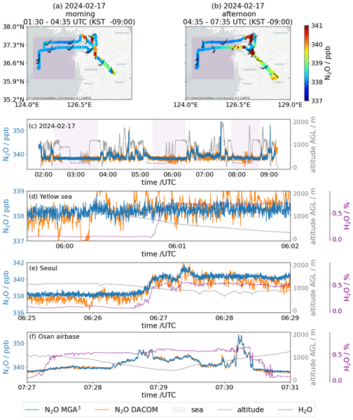
Figure 12 Comparison of color coded N₂O data measured by the MGA³ in the morning in panel (a) and in the afternoon in panel (b) of the same flight in South Korea on 17 February 2024. Panel (c) depicts the time series for the whole flight measured by the MGA³ (10 Hz, precision: 0.17 ppb) and DACOM (5 Hz, precision: 0.3 ppb) and the altitude above ground level showing the frequent ascents and descents. The purple shaded areas show the flight paths over the Yellow Sea in panels (a) and (b), where we measured background concentrations of about 338 ppb in N₂O. Panel (d) shows data from the afternoon over the Yellow Sea where we entered the PBL. The change in water vapor mole fraction while entering seems not to have a significant influence on the water vapor corrected v1-β-off-DLH data and the air seems to be clean enough to show no changes in N₂O compared to the background measurements outside the PBL. The high discrepancies compared to DACOM after 06:00 UTC are attributable to measurement artifacts in the DACOM measurement system due to the implementation of a new detector for N₂O. Panel (e) shows data while entering the PBL over Seoul where enhancements in N₂O can be seen. Panel (f) shows enhancements of up to 16 ppb in N₂O between Pyeongtaek and Anseong approaching Osan Airbase which are in good comparison with the DACOM measurements.

Figure 12 presents an example flight from the campaign in South Korea on the 17 February 2024 and shows the variability of N₂O data as observed on large horizontal scales. Figure 12a and b show the flight tracks for the morning and afternoon flights, respectively, color coded by measured N₂O. The wind barbs indicate southerly to southwesterly winds over the whole flight. In the afternoon (Fig. 12b), slightly higher enhancements can be found than in the morning (Fig. 12a). Especially, the southerly flight path leading west from the land to the sea shows higher enhancements in the afternoon than in the morning. Those enhancements could be caused by the coal fired KOEN Yeonheung Power Plant on Yeonheung island but also by transport from land due to the mainly southerly winds in the afternoon. The correct source attribution is beyond the scope of this work and will be part of an upcoming study. Figure 12c shows the time series of the whole flight with a duration of about 7 h as measured by the MGA³ (10 Hz, precision: 0.17 ppb) and by DACOM (5 Hz, precision: 0.3 ppb). The grey lines represent the flight altitude above ground level (AGL), showing the frequent level changes and vertical profiles between 0 and 2000 m. Over the Yellow Sea west of South Korea, indicated by the purple shaded areas, the N₂O background mole fraction is relatively constant at about 338 ppb. Here, no significant differences within and outside the PBL are observed for N₂O, as shown in more detail in Fig. 12d. A change in H₂O of about 0.7 % is observed when entering the PBL at ∼ 900 m during a descent, while the water vapor corrected N₂O values remain at the same level. The figure also illustrates the better precision and stability of the DLR-MGA³ in comparison to the DACOM instrument. The high discrepancies compared to DACOM after 06:00 UTC are attributable to measurement artifacts in the DACOM measurement system due to the implementation of a new detector for N₂O. In contrast, much higher mole fractions with enhancements of about 3 ppb compared to the background were measured when entering into the PBL over Seoul (Fig. 12e). Finally, Fig. 12f illustrates the general good comparison between the MGA³ data and the DACOM data over larger ranges in N₂O mole fractions, with enhancements of up to 16 ppb as measured during a vertical profile taken close to the Osan Airbase.

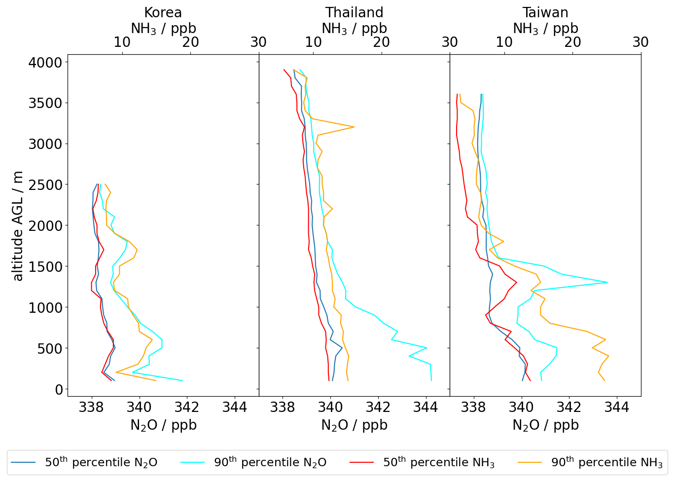
Figure 13 The 50th and 90th percentile of N₂O and NH₃ for South Korea, Thailand and Taiwan. For each country data from all flights are taken to calculate the percentile, except for Taiwan, where we have data from one flight only. In Thailand and Taiwan we had to fly higher than in Korea to get out of the PBL due to higher ambient temperatures. In Korea N₂O and NH₃ show similar behavior. In Thailand the N₂O shows an increase for altitudes below 1500 m due to a rain event in one flight, after which the N₂O emissions were higher over agricultural areas. In general Thailand shows higher enhancements in the PBL for N₂O due to the higher agricultural activities in this region. In Taiwan an increase in N₂O around 1500 m altitude can be seen, which was measured at a technology park at Tainan with manufacturing plants by TSMC.

Using the frequent profiles, we can compare the vertical distribution of N₂O for different regions and also compare it to other species. In the following example, we use NH₃ for comparison, since the agricultural sector is the main anthropogenic source for both species (Behera et al., 2013). The NH₃ was measured by the Los Gatos Research Ammonia Analyzer – Trace (LGR-AAT) (1σ, 0.1 s: 0.7 ppb) operated by the Hankuk University of Foreign Stuies (HUFS) and the National Institute of Environmental Research (NIER) in South Korea. In Fig. 13a, b and c, by using the data from all flights for South Korea and Thailand respectively and a single flight for Taiwan, we calculate the 50th and 90th percentile for N₂O (blue and cyan) and NH₃ (red and orange) for 100 m bins. Each bin has about > 1000 values except for Taiwan with > 100. Due to the warmer temperatures in Thailand and Taiwan compared to South Korea, we generally had to fly higher to scan the PBL completely. For the 50th percentile of N₂O, slightly higher values of 1–2 ppb in Thailand and in Taiwan than in South Korea can be seen for AGL flight altitudes below 1500 and 1000 m, respectively. For the 90th percentile below 1000 m in Thailand, higher values of up to 4 ppb in N₂O compared to South Korea and up to 2 ppb higher than in Taiwan can be seen. One reason for the higher N₂O values in Thailand compared to South Korea could be the impact of lower temperatures on agriculture in South Korea during February. In general, a reason for the high N₂O measured over Thailand could be, that we flew over Central Thailand over a plain stretching from Bangkok to Northern Thailand where agriculture is very prominent and concentrated over thousands of square kilometers. Additionally, on the flight of the 21 March 2024, there was a rain event after which N₂O emission rose in general with enhancements of up to 14 ppb in that area dominating the higher N₂O values for the 90th percentile in Thailand. Those enhancements were measured mainly in agricultural areas. In Taiwan, in the 90th percentile a high enhancement of up to 6 ppb can be seen compared to the background around an altitude of 1000–1700 m. These enhancements with maximum values of 15 ppb originate mainly from the overflights over a technology park divided between the Anding, Shanhua and Xinshi Districts of Tainan where several plants of semiconductor and chip manufacturers like TSMC are located. Additionally, the technology park is surrounded by agricultural fields and contains a waste water treatment facility making this area complex for source attribution. For NH₃, we can see that the 90th percentile in South Korea shows structures similar to those of N₂O. In Taiwan, first, the 50th percentile of NH₃ and the 90th percentile of N₂O seem to match at the altitudes around 1500 m, but then the 90th percentile NH₃ seems to diverge more to higher values for altitudes below 1500 m. For Thailand, NH₃ does not seem to correlate with the N₂O percentiles, especially not with the 90th percentile, although these enhancements in N₂O originate mainly from agricultural regions.

In an already conducted study by Waldmann et al. (2026) at the GHGMon campaign 2023 in the Netherlands, our MGA³ was used for a N₂O eddy covariance study, calculating N₂O fluxes. For a comparison, we applied the same method for specific, representative flux legs across one research flight, once with the v1-β-off water correction and once with the v2 correction, as can be seen in Appendix B and Fig. B1. In the comparison, we could find that the relative difference between the results was around 3 % which is an order of magnitude smaller than the typical relative flux errors reported by Waldmann et al. (2026). Hence, for this instrument setup, we cannot find any significant difference in the influence of the water vapor correction approaches on the calculated eddy covariance fluxes.

6 Summary and Conclusions

In this paper, we evaluate a measurement system for fast (10 Hz) airborne N₂O measurements. The core of the system consists of a commercial QCLAS, the Multicompound Gas Analyzer (MGA³) from MIRO Analytical AG (Switzerland). The system was successfully deployed twice: during the 2023 GHGMon campaign aboard the DLR Cessna with an unpressurized cabin in the Netherlands, and during the 2024 ASIA-AQ campaign aboard NASA's DC-8 with a pressurized cabin over South Korea, Thailand, the Philippines, and Taiwan. The system is calibrated using a two-point calibration every 10 min, with a high and low standard gas for approximately 40 s in total, resulting in a duty cycle of about 94 %. Under this setup, the measuring cell is fully flushed with calibration gas in under 1 s, indicating that the duty cycle could be further increased by reducing the calibration duration.

We operate the instrument in the β-deactivated mode, in which the fitting software freezes the last value used for the width of the spectral profile. By reducing the number of adjustable parameters, this mode decreases the data noise by about 42 % compared to the default β-activated setting. However, because the spectral profile widths are strongly influenced by the highly variable H₂O in the PBL, cross-dependencies on H₂O remain observable in the data.

To correct H₂O dependencies in both the β-deactivated and the β-activated mode, arising from dilution, line broadening, and other spectroscopic effects, we derived an empirical water vapor correction from laboratory experiments which is specific to our individual MGA³ model. We further observed that, from flight to flight, the H₂O measurements show differences relative to NASA's DLH measurements. This is likely due to the inability to perform a two-point calibration of the MGA³-H₂O measurements, as our calibration gases are dry standards. To improve the H₂O correction, we therefore calibrate the MGA³-H₂O measurements against the DLH data leading to the water vapor corrected version of the MGA³ data, namely the v1-β-off-DLH. Also, we tested a new version of the MGA³ fitting software, namely v2, that includes a water vapor correction based on the same laboratory experiments. For H₂O values up to 15 000 ppm, v2 performs comparably to the v1-β-off-DLH, showing similar precision (approximately 0.17 ppb). The v1-β-off-DLH data compares well with N₂O measurements from NASA's DACOM measured simultaneously with our system at the ASIA-AQ campaign even up to 30 000 ppm H₂O. In example data from ASIA-AQ we show that clear differences within large horizontal and vertical scales can be distinguished between different regions with high humidity. We also compare the two approaches v1-β-off and v2 using GHGMon campaign data (Waldmann et al., 2026) to calculate eddy covariance fluxes, but found no significant difference in the resulting fluxes.

We did not observe clear dependencies of the measurements on the aircraft's roll and pitch angles, nor cabin pressure, while sampling calibration gas. However, on the DLR Cessna with its unpressurized cabin, the measurements were generally slightly less stable.

We conclude that the presented instrumental setup enables fast and precise airborne N₂O measurements, suitable for eddy covariance flux estimates and for deployment in highly humid tropical regions.

Appendix A: Dependency of absorption coefficient α on water vapor H₂O

The absorption coefficient α is retrieved from the HITRAN Database 2016 (Gordon et al., 2017). According to the official HITRAN website at https://hitran.org/docs/definitions-and-units/ (last access: 14 October 2026) (Gordon et al., 2022), α is defined as:

$$\begin{array}{}\text{(A1)}& {\mathit{\alpha }}_{i,j}(\mathit{\nu },T,p)=S_{ij}\left(T\right)f(\mathit{\nu },{\mathit{\nu }}_{ij},T,p),\end{array}$$

where S_ij is the intensity of a spectral line for a single molecule for the transition between two states i and j, f the Voigt profile and ν_ij the wavenumber of the spectral line transition in vacuum. The Voigt profile further consists partially of a normalized Lorentz profile f_L defined as:

$$\begin{array}{}\text{(A2)}& f_{\mathrm{L}}(\mathit{\nu },{\mathit{\nu }}_{ij},T,p),={\displaystyle \frac{\mathrm{1}}{\mathit{\pi }}}{\displaystyle \frac{\mathit{\gamma }(p,T)}{\mathit{\gamma }(p,T{)}^{\mathrm{2}}+{\left[\mathit{\nu }-{\mathit{\nu }}_{ij}^{\ast }\left(p\right)\right]}^{\mathrm{2}}}}.\end{array}$$

Here ${\mathit{\nu }}_{ij}^{\ast }$ is the pressure shift corrected wavenumber ν_ij and γ is the Lorentzian Half-Width-Half-Maximum (HWHM) width of the line shape. In the case of pressure broadening on the observed species induced by air, water vapor and the species itself, the resulting width γ is defined as (Kostinek et al., 2019; https://hitran.org/docs/definitions-and-units/):

$$\begin{array}{}\text{(A3)}& \begin{array}{rl}\mathit{\gamma }(p,T)& ={\left({\displaystyle \frac{T_{\mathrm{ref}}}{T}}\right)}^{n_{\mathrm{air}}}\left({\mathit{\gamma }}_{\mathrm{air}}(p_{\mathrm{ref}},T_{\mathrm{ref}})\left(p-p_{\mathrm{self}}-p_{{\mathrm{H}}_{\mathrm{2}}\mathrm{O}}\right)\right.\\ & \left.+{\mathit{\gamma }}_{\mathrm{self}}(p_{\mathrm{ref}},T_{\mathrm{ref}})p_{\mathrm{self}}+{\mathit{\gamma }}_{{\mathrm{H}}_{\mathrm{2}}\mathrm{O}}(p_{\mathrm{ref}},T_{\mathrm{ref}})p_{{\mathrm{H}}_{\mathrm{2}}\mathrm{O}}\right).\end{array}\end{array}$$

Here γ_air, γ_self and ${\mathit{\gamma }}_{{\mathrm{H}}_{\mathrm{2}}\mathrm{O}}$ are the HWHM induced by the partial pressures p_air, $p_{{\mathrm{H}}_{\mathrm{2}}\mathrm{O}}$ and p_self of air, water vapor and the species itself at a reference temperature T_ref=296 K and pressure p_ref=1 atm.

Specifically for the N₂O absorption line used in our MGA³, the HITRAN data base shows that H₂O has a higher broadening effect than air (= nitrogen (N₂), oxygen (O₂)) and N₂O itself with ${\mathit{\gamma }}_{{\mathrm{H}}_{\mathrm{2}}\mathrm{O}}=\mathrm{0.1308}$, γ_air=0.0701 and γ_self=0.085 (Gordon et al., 2022). The difference between γ_self and ${\mathit{\gamma }}_{{\mathrm{N}}_{\mathrm{2}}\mathrm{O}}$ has important implications on the spectral line width. While the global background concentration of N₂O in the troposphere is in the range of about 338 ppb, H₂O mole fractions lie between 1 to 10 ppm even in the dry stratosphere, but can get specifically high in regions such as the tropical boundary layer (up to 30 000 ppm, which is 4 to 5 orders of magnitudes higher than for N₂O. With this, we can simplify Eq. (A3) for measurements in the troposphere to:

$$\begin{array}{}\text{(A4)}& \begin{array}{rl}\mathit{\gamma }(p,T)& ={\left({\displaystyle \frac{T_{\mathrm{ref}}}{T}}\right)}^{n_{\mathrm{air}}}\left({\mathit{\gamma }}_{\mathrm{air}}(p_{\mathrm{ref}},T_{\mathrm{ref}})\left(p-p_{{\mathrm{H}}_{\mathrm{2}}\mathrm{O}}\right)\right.\\ & \left.+{\mathit{\gamma }}_{{\mathrm{H}}_{\mathrm{2}}\mathrm{O}}(p_{\mathrm{ref}},T_{\mathrm{ref}})p_{{\mathrm{H}}_{\mathrm{2}}\mathrm{O}}\right).\end{array}\end{array}$$

Therefore, we assume the width γ of our measured line spectra to be mainly dependent on water vapor for atmospheric measurements in the troposphere, assuming that T and p are constant in the cell.

Appendix B: N₂O Eddy Covariance GHGMon

Waldmann et al. (2026) used the same MGA³ as presented in our study to conduct airborne eddy covariance flux measurements in the course of the GHGMon (Greenhouse Gas Monitoring) campaign 2023 in the Netherlands. Precise high-frequency GHG measurements without interference from water vapor related effects are a prerequisite for robust flux measurements, as water vapor mole fractions are often quite distinct between turbulent updrafts and downdrafts, potentially falsifying GHG measurements if not properly corrected. In order to investigate the extent to which different water vapor correction approaches affect flux measurements, we applied both, the v1-β-off water correction and the v2 correction to specific, representative flux legs across one research flight of the study of Waldmann et al. (2026).

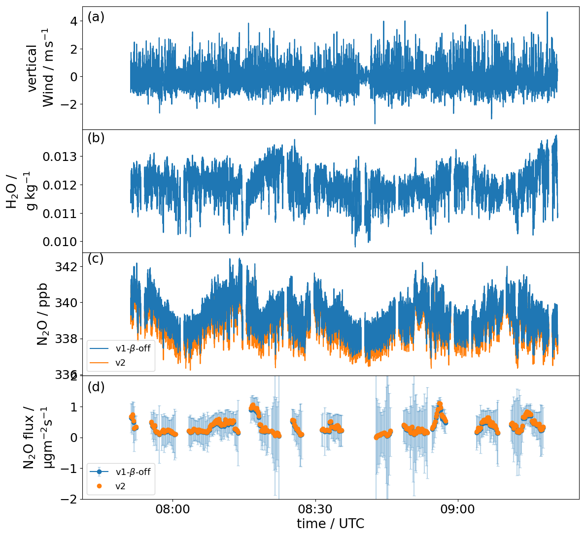
Figure B1 Panel (a) presents vertical wind measurements from a flight on 21 June 2023 in the Netherlands. Panel (b) shows corresponding H₂O measurements. Panel (c) shows the water vapor corrected N₂O measurements, once retrieved with v1-β-off and once with v2. Panel (d) shows the calculated eddy covariance fluxes from the respective time series in panel (c), error bars depicting the uncertainty associated with the flux computation.

In Fig. B1a and b, we can see the vertical wind measurements and the H₂O measurements of the METPOD system on the DLR Cessna from a flight in Friesland on 21 June 2023. Both show high-frequency fluctuations, typical during fair-weather turbulent conditions, which in turn are fundamental for applying the eddy covariance methodology. In Fig. B1c, we see the MGA³-N₂O measurements for the v1-β-off and v2 water correction approaches, similarly showing high-frequency variability expected in the turbulent PBL. In Fig. B1d, the calculated eddy covariance fluxes are shown as time series for the two retrieved mole fractions from Fig. B1c, calculated according to the procedure presented in Waldmann et al. (2026). The mean value for the fluxes over the given time frame is slightly higher for the fluxes with the v2 water correction (0.36 µg m⁻² s⁻¹) compared to the fluxes with the v1-β-off water correction (0.33 µg m⁻² s⁻¹), which translates to a relative difference of 9 %. This difference is expected, given the drift in N₂O corrected according to v2, with increasing H₂O (see Sect. 3.4). However, the relative difference (9 %) is approximately 1 order of magnitude smaller than typical relative flux errors reported in Waldmann et al. (2026), which range between 30 %–100 %, which are superimposed as error bars for the v1-β-off fluxes in Fig. B1d. For both corrections, we computed the limit of detection of N₂O fluxes, which was found to be slightly higher for the v2 water correction with 0.028 µg m⁻² s⁻¹ compared to 0.017 µg m⁻² s⁻¹ for v1-β-off. Given that the differences in fluxes derived with both water vapor corrections is one order of magnitude smaller than typical flux errors, we conclude that the choice of water correction approaches is not a limiting factor for the quality of such flux measurements, but have to be considered when corresponding systems should be improved or small fluxes close to the detection limits are to be measured. We note explicitly that these conclusions are only valid for the comparison of the water vapor corrections presented within this work, and do not represent differences in fluxes calculated with mole fraction measurements with and without water vapor correction.