Physically constrained retrieval of fog visibility from millimeter-wavelength cloud radar observations

Fog severely degrades visibility (Vis) and poses substantial risks to transportation and aviation, yet quantitative monitoring remains challenging because conventional ground-based instruments provide spatially limited point observations and cannot resolve three-dimensional fog structure, while passive satellite retrievals have insufficient vertical resolution and difficulty separating fog from low cloud. Millimeter-wavelength cloud radar (MMCR) can penetrate fog and provide fine spatiotemporal resolution, but many radar Vis retrievals rely on empirical reflectivity–visibility relations. This study develops a physically constrained, observation-calibrated single-wavelength Ka-band MMCR retrieval that links reflectivity, liquid water content (LWC), geometric median radius, extinction, and Vis through lognormal droplet-size-distribution moments. A segment-wise mass-absorption LWC power law and an extinction-oriented radius power law are fitted to same-source FM-120 extinction-matching pseudo-targets, achieving a mean absolute fractional extinction error of 9.37 % on the development dataset. In ten spring-2025 DNQ3-conditioned cases, the present retrieval attains a mean absolute error of 0.092 km, while the local FM-120 and Liu et al. (2019) relations yield broadly comparable ranges and the Gultepe et al. (2009) relation departs more strongly. This method improves the physical self-consistency of single-band MMCR fog Vis retrieval without requiring auxiliary in-situ observations and provides technical support for three-dimensional coastal fog monitoring and traffic meteorological early warning.

1 Introduction

Fog forms when moist air near the surface becomes saturated and water vapor condenses into droplets, often reducing horizontal visibility (Vis) to below 1 km. It is prevalent in valleys and in mountainous, urban, and coastal regions, where radiative cooling, moisture advection, evaporation, or orographic lifting can cause near-surface air to reach saturation. Fog poses substantial risks to port operations, maritime traffic safety, and regional economic activities (Gultepe et al., 2009; Leung et al., 2020; Duran-Rosal et al., 2018). As the core parameter for quantifying fog intensity and guiding operational decisions, Vis is defined as the maximum horizontal distance at which an observer with normal eyesight can distinguish a target against its background under current weather conditions (Middleton, 1957; Long et al., 2021; Miclea et al., 2020). Despite its operational importance, accurate measurement of Vis and characterization of fog structure remain challenging because of limitations in existing observational techniques.

Various instruments have been used to conduct fog observations. Ground-based sensors such as optical visibility meters and fog droplet spectrometers provide high-precision point measurements but fail to capture the horizontal or vertical distribution of fog (Tjugum et al., 2005; Cheng et al., 2018; Zhou et al., 2024). Laser-based active remote-sensing instruments (e.g., lidar, ceilometers) offer vertical profiling capabilities; however, their signals suffer severe attenuation in dense fog, often leading to signal saturation or complete loss (Zang et al., 2019). Satellite passive imagers enable large-scale fog detection but struggle to distinguish fog from low-level clouds and lack vertical resolution to resolve internal stratification or microphysical structures (Ran et al., 2022; Guo et al., 2021). These limitations hinder reliable short-term fog nowcasting and proactive risk mitigation in transportation and maritime operations (Mahdavi et al., 2024; Antoine et al., 2023; Kamangir et al., 2022; Gultepe et al., 2007). In recent years, millimeter-wave cloud radar (MMCR) has gained prominence in fog monitoring due to its strong penetration, fine spatiotemporal resolution, and sensitivity to small hydrometeors. Field campaigns such as the 2021 Pingtan Sea Fog Experiment in China's Fujian Province have shown that Ka-band radar maintains robust signal integrity under dense fog conditions (Hu et al., 2022). Bell (2021) utilized dual-frequency radar to observe multi-layer fog, and by assimilating these radar data into the Applications de la Recherche à l'Opérationnel à Méso-Echelle (AROME) model, they reduced the fog-top height error by 64 % and largely improved visibility forecasts. In the absence of large hydrometeors, MMCR has gained prominence in fog monitoring for its strong penetration, fine resolution, and sensitivity to small hydrometeors (Horvath, 1981; Long et al., 2021; Miclea et al., 2020). The development of millimeter-wave radar has thus provided a new means for fog detection.

Previous studies have advanced the quantification of fog visibility. Early work proposed an inverse relationship between Vis and LWC through bulk microphysical analysis. Subsequent studies showed that DSD strongly modulates extinction and visibility (Eldridge, 1966). Gultepe et al. (2006) incorporated droplet number concentration into a multiparameter scheme, improving Vis estimates in numerical weather prediction models by up to 50 %. Song et al. (2019) further incorporated effective droplet diameter. These studies indicate that fog microphysical properties can improve the physical consistency of visibility estimation (Rui et al., 2023; Jayakumar et al., 2025; Claxton, 2025). Nevertheless, most radar-based Vis parameterizations remain empirical and are commonly obtained by directly fitting Vis to Z (Gultepe et al., 2009). Although Li et al. (2017) introduced radar attenuation correction, the resulting retrieval still relies mainly on empirical relations. Approaches that account for microphysical effects often require auxiliary attenuation or microphysical measurements, restricting operational flexibility where supporting instruments are unavailable.

In this study, we develop a physically based, observation-constrained visibility retrieval algorithm for single-wavelength Ka-band MMCR. Radar transmission theory and fog microphysics provide moment-based links among reflectivity (Z), liquid water content (LWC), effective radius (r_e), and extinction coefficient (β_ext); however, these physical relations alone cannot resolve the ill-posedness inherent in single-wavelength radar measurements. We therefore use five years of FM-120 droplet size distributions as a priori microphysical constraints to inform the retrieval. Specifically, the observed microphysical ranges are used to (i) constrain the initialization and bounds of the mass-absorption-based LWC inversion and (ii) establish an extinction-oriented power-law relationship between the geometric median radius (r_m) and linear reflectivity (Z_lin). Section 2 describes the instrumentation and FM-120 processing. Section 3 presents the theoretical framework, the observed DSD regimes, and the two-step retrieval. Section 4 evaluates retrieval uncertainties associated with DSD shape, the constant-Q_ext approximation, and perturbations in LWC and radius. Section 5 demonstrates the algorithm through a 2025 sea-fog case study and a ten-event consistency comparison. Section 6 summarizes the findings and limitations.

2 Instrumentation and data

Dedicated monitoring campaigns have been conducted at DOB since 2019. The YLUKA2 solid-state Ka-band dual-polarization cloud radar provides reflectivity for the visibility retrieval. A DNQ3 visibility meter provides the near-surface point record for the ten-event consistency comparison, and an FM-120 spectrometer provides DSD and microphysical measurements for algorithm development and sensitivity analysis (Zhang et al., 2024).

The YLUKA2 MMCR is installed at the highest point of DOB, with an antenna height of approximately 25 m. It operates at 34.50–35.50 GHz with an adjustable center frequency and integrates solid-state transmission, dual-transmitter/dual-receiver linear polarization, and fully coherent pulse-Doppler technology. Manufacturer specifications list 30 m spatial resolution, a 30 km maximum detection range, a 42 dB ground-clutter suppression ratio, and a minimum detectable reflectivity factor of −30 dBZ at 10 km. The YLUKA2 MMCR performs sector Plan Position Indicator (PPI) scans at a fixed elevation angle of 2°, conducting continuous azimuthal surveillance between 60 and 300°. The YLUKA2 MMCR data used in this study are primarily affected by clear-sky ground clutter. As this method places high demands on data continuity, we recorded the ground clutter under clear-sky conditions and subsequently subtracted this clutter contribution to complete the ground clutter removal (Li et al., 2013; Boers et al., 2013; Kanemaru et al., 2021).

The FM-120 operated continuously from 2019 through 2023. It measures droplets from 2–50 µm at 1 Hz in 30 non-equidistant size bins. The DSD observations are used to derive fog microphysical parameters, including β_ext, LWC, and r_m, for algorithm development and sensitivity analysis.

The DNQ3 visibility meter operates on the forward-scattering principle. It emits infrared pulses with a central wavelength of 0.87 µm, and the sensor receives light scattered at a forward angle. The instrument is approximately 153 m from the radar along azimuth 150°. Because this position is near the radar's minimum range, a nearby radar point whose temporal variation is most consistent with the DNQ3 trend is selected for matching. The ten spring-2025 cases were included when DNQ3 visibility remained continuously below 1000 m for at least 30 min and no other precipitation weather occurred during the interval.

The DOB location and MMCR installation are shown in Fig. 1.

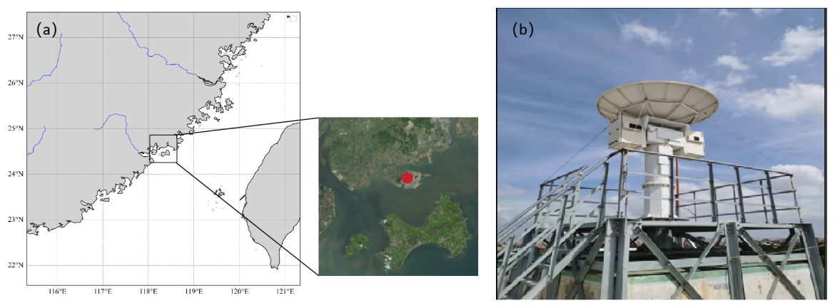
Figure 1 (a) Geographical location of DOB in Xiang'an District, Xiamen. The red mark denotes the observation station. The base map of the regional overview is provided by corresponding author Qiaoyi Lv; the inset satellite imagery is sourced from Baidu Maps, © Baidu Inc., used for academic research only. (b) The YLUKA2 MMCR installation at the observation site.

2.1 FM-120 processing and observational constraints

The FM-120 fog droplet spectrometer operated at the Datan Observation Base from 2019 through 2023. It measured droplets over a nominal diameter range of 2–50 µm in 30 non-equidistant channels at 1 Hz.

A new event was defined when the gap between consecutive valid minutes exceeded 30 min. After quality control, the spectral-regime dataset aggregates 236037 contributing 1 Hz records into 4234 valid 1 min spectra from 28 events by summing particle counts and dividing by the summed sampling volume. For channel i, the 1 min number concentration was $N_i=C_i/V_{\mathrm{s}}$, where C_i is the particle count and V_s is sampled volume. With D_i in metres, D_i in millimetres, N(D) in m⁻³ mm⁻¹, and N_T in m⁻³, the discrete calculations were

$$\begin{array}{}\text{(1)}& \begin{array}{rl}\mathrm{LWC}& ={\displaystyle \frac{{\mathrm{10}}^{\mathrm{3}}}{{\mathit{\rho }}_w}}\sum _i{N}_i{\displaystyle \frac{\mathrm{4}\mathit{\pi }}{\mathrm{3}}}{r}_i^{\mathrm{3}}[\mathrm{g}/{\mathrm{m}}^{\mathrm{3}}],\\ Z_{\mathrm{lin}}& =\sum _i{N}_i{D}_i^{\mathrm{6}}[{\mathrm{mm}}^{\mathrm{6}}/{\mathrm{m}}^{\mathrm{3}}],\\ {\mathit{\beta }}_{\mathrm{ext}}& =\sum _i{N}_i{Q}_{\mathrm{ext},i}\mathit{\pi }{r}_i^{\mathrm{2}}[/\mathrm{m}],\\ r_{\mathrm{e}}& ={\displaystyle \frac{{\sum }_i{N}_i{r}_i^{\mathrm{3}}}{{\sum }_i{N}_i{r}_i^{\mathrm{2}}}},\end{array}\end{array}$$

where Q_ext,i is the size-dependent Mie extinction efficiency evaluated at 550 nm. Total number concentration and the number-weighted radius summary were obtained from the same discrete spectrum. All of these quantities share the same DSD source and therefore provide sample-internal conditioning variables rather than independent visibility observations; no separate historical interpolation or concentration-residual processing chain is implied by Eq. (1).

3 Observation-constrained retrieval development

The classical Koschmieder law (Koschmieder, 1924; Horvath, 1971) expresses Vis as

$$\begin{array}{}\text{(2)}& \mathrm{Vis}=-{\displaystyle \frac{\ln \mathit{\epsilon }}{{\mathit{\beta }}_{\mathrm{ext}}}}=-{\displaystyle \frac{\ln \mathrm{0.02}}{{\mathit{\beta }}_{\mathrm{ext}}}}\end{array}$$

where ε is the brightness-contrast threshold, typically set to 0.02, and β_ext is the extinction coefficient (unit: m⁻¹) at 550 nm. According to Mie scattering theory,

$$\begin{array}{}\text{(3)}& {\mathit{\beta }}_{\mathrm{ext}}=\underset{\mathrm{0}}{\overset{\mathrm{\infty }}{\int }}{Q}_{\mathrm{ext}}(r,\mathit{\lambda })n\left(r\right)\mathit{\pi }{r}^{\mathrm{2}}\mathrm{d}r\end{array}$$

where Q_ext is the extinction efficiency for a droplet of radius r, and n(r) is the fog DSD (unit: m⁻⁴), which is commonly represented by a lognormal distribution (Bernardin et al., 2010; Podzimek, 1997):

$$\begin{array}{}\text{(4)}& n\left(r\right)={\displaystyle \frac{N_{\mathrm{T}}}{\sqrt{\mathrm{2}\mathit{\pi }}r\mathit{\sigma }}}\exp \left[{\displaystyle \frac{-{\ln }^{\mathrm{2}}(r/r_{\mathrm{m}})}{\mathrm{2}{\mathit{\sigma }}^{\mathrm{2}}}}\right]\end{array}$$

Here, N_T is total droplet number concentration, r_m is geometric median radius, and σ is logarithmic spectral width. For a lognormal distribution, the kth DSD moment can be written as

$$\begin{array}{}\text{(5)}& M_k=N_{\mathrm{T}}{r}_{\mathrm{m}}^k\exp \left({\displaystyle \frac{k^{\mathrm{2}}{\mathit{\sigma }}^{\mathrm{2}}}{\mathrm{2}}}\right)\end{array}$$

MMCR operates in the millimetre-wave band, where most fog droplets are in the Rayleigh regime. The attenuation-corrected radar reflectivity factor Z is proportional to the sixth DSD moment:

$$\begin{array}{}\text{(6)}& Z=\mathrm{64}{M}_{\mathrm{6}}=\mathrm{64}{N}_{\mathrm{T}}{r}_{\mathrm{m}}^{\mathrm{6}}\exp \left(\mathrm{18}{\mathit{\sigma }}^{\mathrm{2}}\right)\end{array}$$

Because Z and β_ext depend on different DSD moments, they cannot be linked uniquely without intermediate microphysical information. LWC and effective radius are defined by

$$\begin{array}{}\text{(7)}& {\displaystyle }\mathrm{LWC}={\displaystyle \frac{\mathrm{4}}{\mathrm{3}}}\mathit{\pi }{\mathit{\rho }}_{\mathrm{w}}{M}_{\mathrm{3}}={\displaystyle \frac{\mathrm{4}}{\mathrm{3}}}\mathit{\pi }{\mathit{\rho }}_{\mathrm{w}}{N}_{\mathrm{T}}{r}_{\mathrm{m}}^{\mathrm{3}}\exp \left({\displaystyle \frac{\mathrm{9}}{\mathrm{2}}}{\mathit{\sigma }}^{\mathrm{2}}\right)\text{(8)}& {\displaystyle }{r}_{\mathrm{e}}={\displaystyle \frac{M_{\mathrm{3}}}{M_{\mathrm{2}}}}=r_{\mathrm{m}}\exp \left({\displaystyle \frac{\mathrm{5}}{\mathrm{2}}}{\mathit{\sigma }}^{\mathrm{2}}\right)\end{array}$$

where ρ_w is water density. Eliminating N_T and σ from the moment relations gives (Du et al., 2024; Stephens, 1978)

$$\begin{array}{}\text{(9)}& r_{\mathrm{e}}=r_{\mathrm{m}}^{\frac{\mathrm{4}}{\mathrm{9}}}{\left({\displaystyle \frac{\mathit{\pi }{\mathit{\rho }}_{\mathrm{w}}Z}{\mathrm{48}\mathrm{LWC}}}\right)}^{\frac{\mathrm{5}}{\mathrm{27}}}\end{array}$$

In the visible band, the extinction efficiency of sufficiently large fog droplets approaches 2 (Mazoyer et al., 2022). Figure 2 shows its radius dependence at 550 nm.

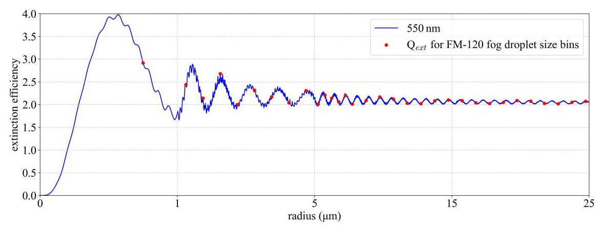
Figure 2 Size dependence of Q_ext at 550 nm. Red points mark radii associated with the FM-120 size bins. The constant value Q_ext=2 is an asymptotic approximation rather than an exact representation over the sampled small-droplet range.

For Q_ext≈2, extinction is $\mathrm{3}\mathrm{LWC}/\left(\mathrm{2}{\mathit{\rho }}_{\mathrm{w}}{r}_{\mathrm{e}}\right)$. Substitution of Eq. (9) gives

$$\begin{array}{}\text{(10)}& {\mathit{\beta }}_{\mathrm{ext}}={\displaystyle \frac{\mathrm{3}\mathrm{LWC}}{\mathrm{2}{\mathit{\rho }}_{\mathrm{w}}{r}_{\mathrm{e}}}}={\displaystyle \frac{\mathrm{3}}{\mathrm{2}{\mathit{\rho }}_{\mathrm{w}}}}{r}_{\mathrm{m}}^{-\frac{\mathrm{4}}{\mathrm{9}}}{\left({\displaystyle \frac{\mathit{\pi }{\mathit{\rho }}_{\mathrm{w}}Z}{\mathrm{48}}}\right)}^{-\frac{\mathrm{5}}{\mathrm{27}}}{\mathrm{LWC}}^{\frac{\mathrm{32}}{\mathrm{27}}}.\end{array}$$

All quantities are evaluated in consistent SI units, including ρ_w, LWC, radius, and the conventional mm⁶ m⁻³ reflectivity factor. Combining Eq. (10) with Koschmieder's relation yields

$$\begin{array}{}\text{(11)}& \mathrm{Vis}=\mathrm{3.91}{\displaystyle \frac{\mathrm{2}{\mathit{\rho }}_{\mathrm{w}}}{\mathrm{3}}}{r}_{\mathrm{m}}^{\frac{\mathrm{4}}{\mathrm{9}}}{\left({\displaystyle \frac{\mathit{\pi }{\mathit{\rho }}_{\mathrm{w}}Z}{\mathrm{48}}}\right)}^{\frac{\mathrm{5}}{\mathrm{27}}}{\mathrm{LWC}}^{-\frac{\mathrm{32}}{\mathrm{27}}}.\end{array}$$

Equation (10) requires both LWC and r_m, neither of which is uniquely determined by one MMCR reflectivity measurement. We therefore use two observation-constrained steps. The mass-absorption/TRR routine retrieves LWC and applies liquid-water attenuation correction, and the FM-120 development data provide the conditional radius–reflectivity relations.

3.1 FM-120-observed spectral regimes and retrieval context

This section characterizes the morphology of fog droplet size distributions (DSDs) and the variation of microphysical parameters across fog intensity grades, drawing on long-term FM-120 observations. The results provide observational constraints for the visibility-retrieval parameterization developed in subsequent sections and delineate the applicability boundary of the single-lognormal closure assumption.

3.1.1 Data processing and spectral shape classification

Following standard classification criteria for fog DSD morphology, each 1 min spectrum is assigned to one of four definite shape categories: narrow unimodal, broad unimodal, shoulder, and bimodal. An additional uncertain status is reserved for samples with indistinct morphological features: spectra with a stability score below 0.80 are labeled as uncertain. Among them, 584 samples exhibit a weak two-peak pattern but are not classified as bimodal due to insufficient peak separation.

Across the full dataset, shoulder and broad-unimodal spectra account for the largest proportions, at 41.83 % and 33.54 %, respectively. Bimodal spectra make up 6.38 %, and narrow-unimodal spectra account for 4.32 %. The remaining 13.93 % fall into the uncertain status. Median normalized spectra and interquartile ranges for each shape category are shown in Fig. 3a. Narrow-unimodal spectra have the smallest peak diameter and narrowest spectral width, while bimodal spectra exhibit a primary mode near 5 µm and a secondary mode near 25 µm, with an overall spectral width substantially larger than that of unimodal spectra.

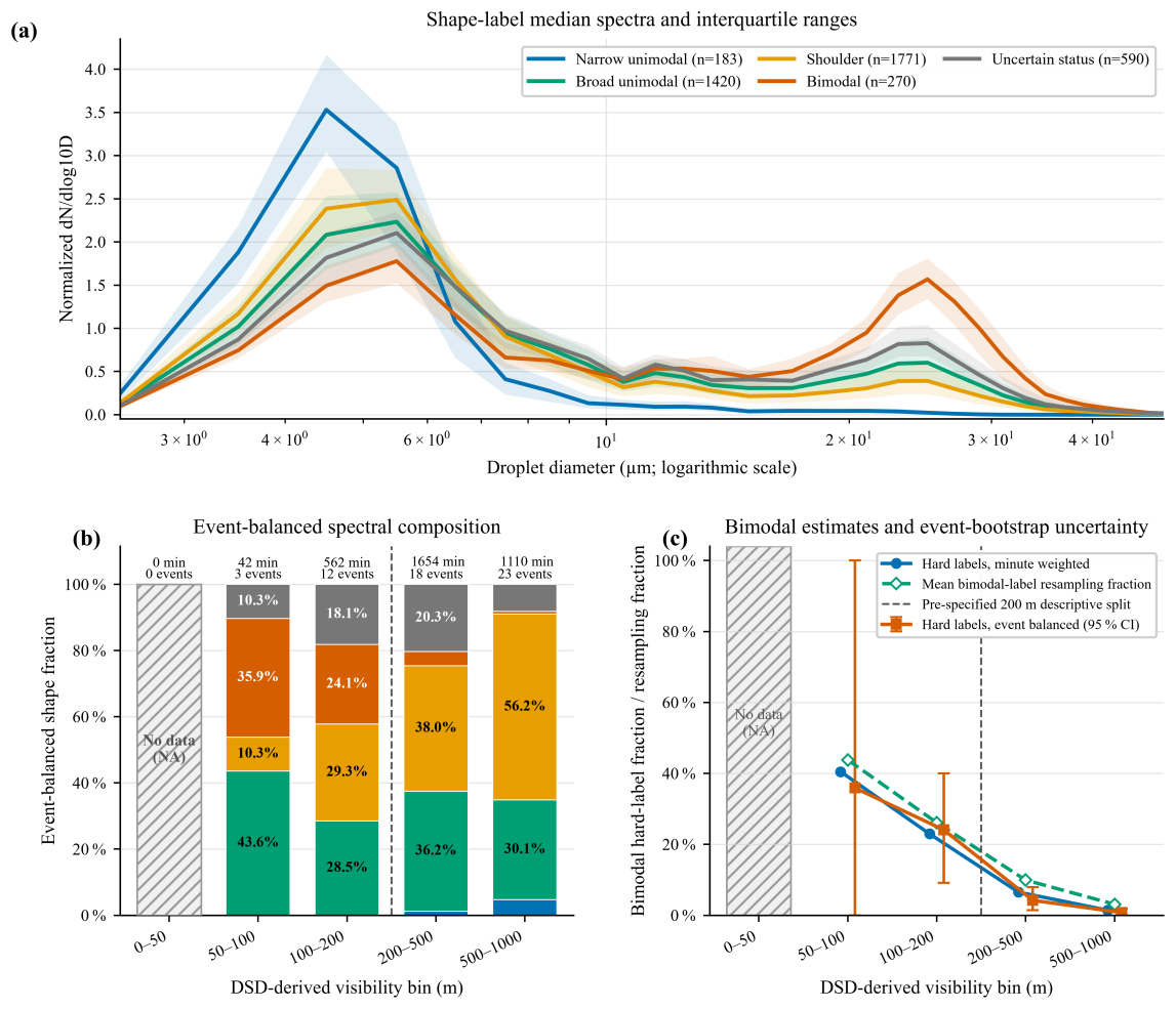
Figure 3 FM-120 spectral summaries from the spectral-regime dataset. (a) Median normalized spectra and interquartile ranges by fixed shape label. (b) Event-balanced hard-label composition in DSD-derived visibility bins; the dashed line marks the pre-specified 200 m split. (c) Minute-weighted, event-balanced, and label-resampling bimodal summaries.

3.1.2 Evolution of spectral shapes across visibility grades

To examine how DSD shapes vary with fog intensity, samples are grouped into four visibility grades according to meteorological fog classification standards, based on DSD-derived visibility: heavy fog (500 m $\le V<\mathrm{1000}$ m), dense fog (200 m $\le V<\mathrm{500}$ m), very dense fog (50 m $\le V<\mathrm{200}$ m), and extremely dense fog (V<50 m). An event-balanced statistical approach is applied: the fraction of each shape category within each visibility bin is first calculated per event, then averaged across all events with equal event weights. The spectral shape composition across visibility grades is presented in Fig. 3b.

Statistical results show that the proportion of bimodal spectra rises markedly as visibility decreases: Heavy fog (500–1000 m): bimodal spectra account for only 0.77 % (95 % confidence interval: 0.03 %–1.79 %), with unimodal and shoulder shapes dominating; Dense fog (200–500 m): the bimodal fraction increases to 4.22 % (95 % confidence interval: 1.45 %–7.96 %); Very dense fog (100–200 m): the bimodal fraction jumps to 24.07 % (95 % confidence interval: 9.11 %–40.04 %); The 50–100 m bin yields a point estimate of 35.90 % bimodal fraction, but only 3 events contribute to this interval with a confidence interval spanning 0 %–100 %, so it is not used for robust quantitative inference.

No DSD samples are available for the extremely dense fog (0–50 m) grade in this dataset. Overall, when visibility falls below 200 m, the deviation of fog DSD from a single lognormal distribution becomes pronounced, and bimodal structures emerge as a non-negligible spectral feature. Figure 3c also presents bimodal fractions under alternative statistical frameworks (minute-weighted, event resampling), all of which show consistent trends.

3.1.3 Comparison of microphysical parameters between two visibility strata

Building on the 200 m visibility threshold identified above, samples are further divided into a low-visibility stratum ($\mathrm{0}<V_{\mathrm{Mie}}\le \mathrm{200}$ m) and a high-visibility stratum (200 m $<V_{\mathrm{Mie}}\le \mathrm{1000}$ m). We compare the distribution of five microphysical parameters between the two strata: radar-equivalent reflectivity factor Z, total number concentration N_T, liquid water content (LWC), effective radius r_e, and geometric median radius r_m, as illustrated in Fig. 4.

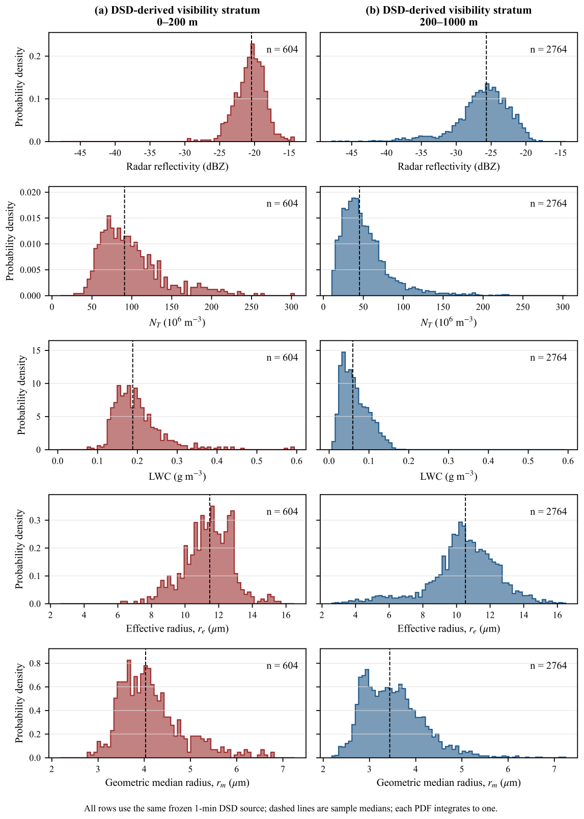
Figure 4 Timestamp-resolved FM-120 parameter distributions in the pre-specified strata (a) $\mathrm{0}<V_{\mathrm{Mie}}\le \mathrm{200}$ m and (b) 200 m $<V_{\mathrm{Mie}}\le \mathrm{1000}$ m. Rows show FM-120/DSD-derived radar-equivalent Z (dBZ), N_T (m⁻³), LWC (g m⁻³), r_e (µm), and the visibility-workflow geometric-median-radius proxy r_m (µm). Each histogram is normalized within its stratum; dashed lines denote sample medians.

Distinct microphysical differences are observed between the two strata. The median Z in the low-visibility stratum is −2.61 dBZ, 4.92 times the value of −9.53 dBZ in the high-visibility stratum, a difference of approximately 6.92 dBZ corresponding to a 4.92-fold increase.

The median N_T and LWC in the low-visibility stratum are 97.31×10⁶ m⁻³ and 0.21 g m⁻³, 2.19 times and 3.83 times the values in the high-visibility stratum (44.34×10⁶ m⁻³, 0.06 g m⁻³), respectively, also showing strong discriminative power.

Differences in radius parameters between the two strata are comparatively small. The geometric median radius r_m and effective radius r_e in the low-visibility stratum are 13.57 and 11.90 µm, only 0.83 and 1.55 µm larger than in the high-visibility stratum, with far weaker separability than reflectivity and LWC.

3.2 Mass-absorption-constrained LWC retrieval

In the visibility parameterization, accurate retrieval of liquid water content (LWC) and unattenuated radar reflectivity factor Z are essential. Therefore, we adopted the self-consistent LWC retrieval algorithm developed in Ge's research (Ge et al., 2023) to calculate LWC, and correct the absorption attenuation in the measured radar reflectivity Z_m.

The attenuation of millimeter-wave radar signals during propagation in fog is mainly caused by mass absorption of water droplets. Under the Rayleigh approximation, one-way liquid-water attenuation is proportional to LWC, $A=K^{*}\mathrm{LWC}$, independent of the droplet size distribution. Here, K^* is determined by the radar wavelength, temperature, and complex refractive index of cloud droplets, and can be treated as a constant for a millimeter-wave radar operating at a fixed wavelength. Based on this, a self-consistent LWC retrieval framework is adopted: the radar radiative transfer equation is transformed into a Bernoulli differential equation and integrated within the cloud layer to establish a constrained relationship among the measured reflectivity factor Z_m, the true reflectivity factor Z, and LWC. To obtain a closed-form solution, a segment-wise power-law relation is employed as a numerical closure. A bounded trust-region reflective (TRR) least-squares solver is used to optimize the parameter vector by minimizing the absolute dBZ residual between the measured and reconstructed reflectivity (Cartis et al., 2009). The reconstructed reflectivity is expressed as

$$\begin{array}{}\text{(12)}& Z_{\mathrm{mc},{\mathrm{r}}_i}=c{\mathrm{LWC}}_{{\mathrm{r}}_i}^{\frac{\mathrm{1}}{b}}\exp \left(-\mathrm{0.46}\underset{r_{\mathrm{0}}}{\overset{r_i}{\int }}{K}^{*}\mathrm{LWC}\left(s\right)\mathrm{d}s\right).\end{array}$$

where the effect of gaseous attenuation on radiative transfer is neglected. Once LWC is retrieved, the accumulated attenuation can be readily computed and applied to correct the measured reflectivity. Given the substantial variability in liquid water path (LWP) along fog profiles detected by radar – as noted in Sect. 3.1, bimodal fog events exhibit significant enhancements in both Z and LWC – a 10-bin segmentation approach is applied to partition the profile into segments such that the LWP of each segment falls within the bounds prescribed by the TRR method. The numerical branch is selected according to the maximum original reflectivity within each segment: for a maximum not exceeding −15 dBZ, the starting vector is $[\mathrm{0.5},\mathrm{0.01},\mathrm{1}]$; for a maximum greater than −15 dBZ, it is $[\mathrm{0.5},\mathrm{0.01},\mathrm{0.1}]$. Both branches use lower bounds $[\mathrm{0},\mathrm{0},\mathrm{0}]$ and upper bounds $[\mathrm{1},\mathrm{1},\mathrm{10}]$. Each segment is fitted independently, with the accumulated attenuation derived from the retrieved LWC applied to its reflectivity prior to fitting. This approach requires neither ancillary instruments nor empirical coefficients, achieving LWC retrieval and attenuation correction through the self-consistent interdependencies among cloud physical variables.

3.3 Extinction-oriented conditional parameterization of r_m

In addition to accurate LWC retrieval, determining r_m is a critical step. Although observational studies on r_m have been conducted previously, no empirical relationship between r_m and Z has been established for fog. Given that both r_m and Z are intimately linked to DSD, a strong power-law correlation is expected. Herein, we adopt the power-function form r_m=aZ^b to parameterize this relationship.

A single-frequency reflectivity measurement cannot determine r_m uniquely because total number concentration and spectral width also affect the sixth DSD moment. We therefore compare two sample-internal conditional parameterizations. The direct radius-space fit is used only as a comparison baseline. The selected extinction-oriented relation is fitted to extinction-matching pseudo-targets in the moment-closure development dataset; the pseudo-targets are constructed from reflectivity, LWC, and size-dependent Mie extinction co-derived from the same FM-120 DSD.

For each development row i, candidate radii from 1.00 to 20 µm at 0.01 µm spacing were inserted into Eq. (10). The row-wise extinction-matching pseudo-target was

$$\begin{array}{}\text{(13)}& r_{\mathit{\beta },i}^{\star }=\arg \underset{r\in \mathcal{G}}{min}{\displaystyle \frac{\left|{\mathit{\beta }}_{\mathrm{ext},\mathrm{closed}}\right(r;Z_{\mathrm{lin},i},{\mathrm{LWC}}_i)-{\mathit{\beta }}_{\mathrm{ext},\mathrm{FM}\mathrm{120},i}|}{{\mathit{\beta }}_{\mathrm{ext},\mathrm{FM}\mathrm{120},i}}},\end{array}$$

where 𝒢 is the finite candidate grid. Thus $r_{\mathit{\beta },i}^{\star }$ is a constructed radius pseudo-target, not an independently observed geometric median radius. A free power law was then fitted to these pseudo-targets by unweighted radius-space least squares:

$$\begin{array}{}\text{(14)}& {\displaystyle \frac{r_{\mathrm{m}}}{\mathit{\mu }\mathrm{m}}}=\mathrm{21.87}{\left[{\displaystyle \frac{Z_{\mathrm{lin}}}{{\mathrm{mm}}^{\mathrm{6}}/{\mathrm{m}}^{\mathrm{3}}}}\right]}^{\mathrm{0.20}}.\end{array}$$

Linear Z_lin is the predictor for both relations, whereas dBZ is used only as a plotting coordinate. Against their respective fit targets, the direct relation has same-sample Pearson R=0.74 and RMSE 0.86 µm, and the extinction-oriented relation has R=0.73 and pseudo-target RMSE 1.64 µm. Figure 5 displays the direct comparison baseline in panel (a) and the selected extinction-oriented relation in panel (b).

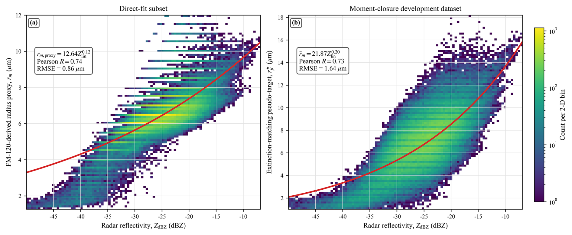
Figure 5 Sample-internal radius–reflectivity fits. (a) Direct-fit subset with the FM-120-derived radius proxy. (b) Moment-closure development dataset with row-wise extinction-matching pseudo-targets. Linear Z_lin is fitted, while dBZ is the display coordinate; equations, same-sample Pearson R, and radius RMSE are shown to two decimal places.

4 Evaluation of retrieval assumptions and uncertainties

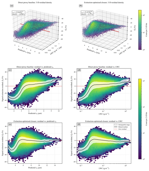
The retrieval framework constructed in Sect. 3 reduces reliance on direct visibility–reflectivity fitting, but its accuracy is ultimately governed by two algorithmic assumptions. The first is the constant extinction-efficiency approximation (Q_ext=2), which replaces the size-dependent Mie efficiency shown in Fig. 2 with its large-particle asymptote. The second is the single-lognormal closure, which constrains the droplet size distribution to a parametric form that links reflectivity, liquid water content, and effective radius through shared moments. Both assumptions introduce structural biases whose magnitude depends on droplet size and spectral modality. Section 4.1 attributes the extinction-residual patterns revealed in Fig. 6 to these two sources: the weak-reflectivity bias is traced to the Q_ext=2 approximation, while the broader residual reflects the lognormal closure and is partially mitigated by the extinction-oriented parameterization. Section 4.2 quantifies the analytical sensitivity of the retrieved extinction to perturbations in LWC and radius.

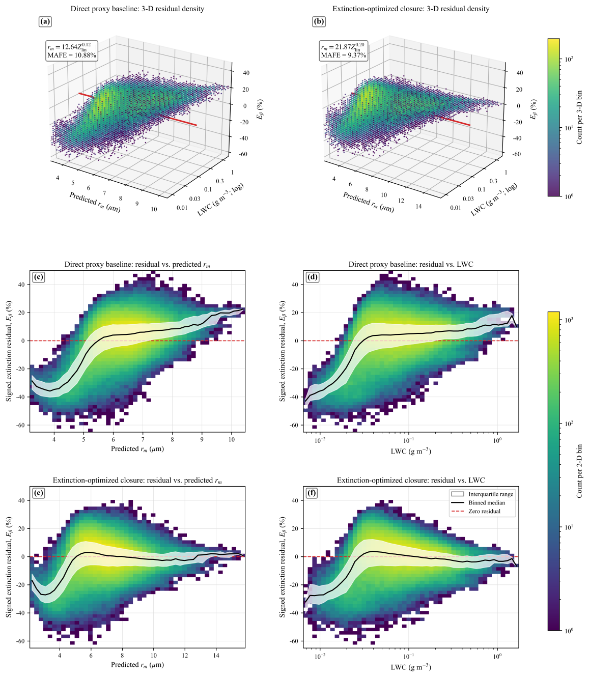
Figure 6 Same-sample extinction-residual distributions for the moment-closure development dataset. (a, b) Three-dimensional residual density for the direct and extinction-oriented relations. (c, d) Direct-relation residual versus predicted radius and LWC; (e, f) corresponding extinction-oriented views. In (c)–(f), colour denotes count per bin, white bands the interquartile range, and black curves the binned median; red references mark zero residual, and both methods share the residual scale.

4.1 DSD effects on the radius–reflectivity relation and extinction retrieval

The DSD primarily affects the retrieval through the radius term.

To quantify the response to this structural variability, the direct and extinction-oriented relations are evaluated on the moment-closure development dataset. For each relation, the predicted radius is inserted into Eq. (10) with the same row's Z_lin and LWC and compared with the same size-dependent Mie extinction reference. All quantities are same-sample and deterministic; there is no held-out subset or independent physical-radius observation. Accordingly, all R, RMSE, signed-residual, and MAFE values in Sects. 3.3 and 4.1 are resubstitution diagnostics that measure numerical consistency with the development targets. The signed fractional residual and mean absolute fractional error (MAFE) are

$$\begin{array}{}\text{(15)}& {\displaystyle }{E}_{\mathit{\beta },i}={\displaystyle \frac{{\widehat{\mathit{\beta }}}_{\mathrm{ext},i}-{\mathit{\beta }}_{\mathrm{ext},\mathrm{FM}\mathrm{120},i}}{{\mathit{\beta }}_{\mathrm{ext},\mathrm{FM}\mathrm{120},i}}}\times \mathrm{100}\mathit{\%},\text{(16)}& {\displaystyle }\mathrm{MAFE}={\displaystyle \frac{\mathrm{1}}{N}}\sum _{i=\mathrm{1}}^N\left|E_{\mathit{\beta },i}\right|.\end{array}$$

where N is the total number of rows in the moment-closure development dataset. For the $Z_{\mathrm{dBZ}}<-\mathrm{40}$ subset, the signed mean of E_β is −25.32 %. The negative sign means that the closed-form extinction is lower on average than the same-row FM-120/Mie extinction; because visibility is inversely proportional to extinction, the closed-form result therefore tends toward visibility overestimation in this subset. This same-row, same-source signed mean is not an independent error estimate and is distinct from the signed mean and 22.01 % MAFE for the broader $-\mathrm{50}\le Z_{\mathrm{dBZ}}<-\mathrm{35}$ interval. The bimodal error structure visible in Fig. 6 can be attributed to the two algorithmic assumptions identified above. For weak-reflectivity cases, the predicted radii fall predominantly below 5 µm, a range in which the actual Mie extinction efficiency at 550 nm deviates most strongly from the assumed constant value of 2 (Fig. 2). Because the constant-Q_ext approximation enters the analytical closure linking extinction to LWC and radius (Eq. 10), this deviation systematically biases the closed-form extinction downward relative to the size-dependent Mie reference in the small-radius regime. The resulting extinction underestimation is consistent with the pronounced negative signed residual and elevated MAFE (22.01 %) observed in the weak-reflectivity bin of Fig. 6. The residual that persists across the remaining reflectivity range arises primarily from the single-lognormal assumption: when the observed DSD departs from lognormality, as occurs increasingly at visibilities below 200 m where bimodal spectra become prevalent (Sect. 3.1), the moment-based closure relating reflectivity, LWC, and radius no longer holds exactly. The extinction-oriented parameterization was designed to reduce precisely this distribution-shape error: by calibrating the radius–reflectivity relation against extinction-matching pseudo-targets rather than direct geometric radius proxies, it absorbs part of the departure from lognormality into the empirical power-law coefficients. The reduction in overall MAFE from 10.88 % to 9.37 %, and most notably from 12.25 % to 4.96 % at intermediate reflectivities, confirms the effectiveness of this strategy. The weak-reflectivity residual, however, is dominated by the Q_ext approximation and is not substantially improved by the extinction-oriented fitting alone.

Across the moment-closure development dataset, the direct relation yields an extinction MAFE of 10.88 %, whereas the extinction-oriented relation yields 9.37 %. The largest decrease occurs for $-\mathrm{15}\le Z_{\mathrm{dBZ}}<\mathrm{0}$, from 12.25 % to 4.96 %.

4.2 Analytical sensitivity to LWC and r_m

In practical application of the algorithm, reliable retrievals of LWC, Z, and r_e are essential for accurate visibility calculation via Eq. (10). On one hand, the fog DSD does not strictly follow the lognormal distribution and may exhibit bimodal or multimodal characteristics, which introduces uncertainties into the calculation. On the other hand, both LWC and r_m are derived from Z – while Z is simultaneously corrected during LWC retrieval via the self-consistent algorithm, residual deviations between the retrieved LWC and its true value still exist. Additionally, the corrected Z is influenced by LWC, which further propagates uncertainties to r_m. Furthermore, r_m itself is an estimated parameter, with a RMSE of 1.64 µm as shown in the validation results (Fig. 5). To quantify the impact of these uncertainties on algorithm performance, we conducted perturbation simulations on both the retrieved LWC and empirically derived r_m, with a focus on analyzing the resulting characteristics of retrieval errors. We define a relative extinction response f that characterizes how retrieval extinction errors respond to perturbations in these two parameters. Let α and λ be multiplicative perturbations to r_m and LWC. From Eq. (10),

$$\begin{array}{}\text{(17)}& {\mathit{\beta }}_{\mathrm{ext},\mathrm{pert}}={\mathit{\beta }}_{\mathrm{ext}}{\mathit{\alpha }}^{-\frac{\mathrm{4}}{\mathrm{9}}}{\mathit{\lambda }}^{\frac{\mathrm{32}}{\mathrm{27}}},\end{array}$$

so the relative extinction response is

$$\begin{array}{}\text{(18)}& f={\displaystyle \frac{{\mathit{\beta }}_{\mathrm{ext},\mathrm{pert}}-{\mathit{\beta }}_{\mathrm{ext}}}{{\mathit{\beta }}_{\mathrm{ext}}}}={\mathit{\alpha }}^{-\frac{\mathrm{4}}{\mathrm{9}}}{\mathit{\lambda }}^{\frac{\mathrm{32}}{\mathrm{27}}}-\mathrm{1}.\end{array}$$

Ge et al. (2023) reported that retrieved LWC can deviate from its true value by 50 % to 200 % under the self-consistent mass-absorption algorithm. In this study, the same fractional range applies to the empirically derived r_m. Both multipliers (α and λ) are therefore varied from 0.50 to 2.00, spanning the physically plausible uncertainty range of these two parameters. Figure 7 displays the complete response range with a zero-centred normalization. The zero-response curve is $\mathit{\lambda }={\mathit{\alpha }}^{\mathrm{3}/\mathrm{8}}$; same-signed perturbations partly compensate because radius and LWC enter with opposite-signed exponents. The larger LWC exponent produces a stronger analytical response to LWC perturbations. The ratio of the exponent magnitudes is $(\mathrm{22}/\mathrm{27})/(\mathrm{4}/\mathrm{9})=\mathrm{11}/\mathrm{6}\approx \mathrm{1.83}$, meaning that for any given fractional perturbation, the extinction response to LWC is approximately twice that of r_m. For instance, a 10 % increase in LWC raises the extinction by 8.1 %, whereas a 10 % increase in r_m lowers it by only 4.1 %. In practice, drizzle-sized droplets (diameter >100 µm) may appear near the fog top or during the mature-to-dissipation stage. Because the mass-absorption retrieval of LWC depends on the integrated liquid water mass (third DSD moment) rather than the sixth-moment reflectivity, it is intrinsically less sensitive to sparse large droplets; the attenuation coefficient k remains closely tied to the bulk LWC, and no pronounced overestimation is expected. This is consistent with Fig. 7, which shows that LWC perturbations dominate the extinction response. By contrast, the extinction-oriented r_m–Z relation (Sect. 3.3) is calibrated against the FM-120 dataset, whose upper measurement limit is 50 µm. When drizzle droplets dominate the radar sampling volume, they disproportionately increase reflectivity while contributing modestly to the geometric median radius inferred from the FM-120-constrained power law. Consequently, the parameterized r_m may be systematically biased high. Because r_m enters the visibility retrieval with a negative exponent (Eq. 10), an overestimated r_m reduces the inferred extinction, partially offsetting the enhanced extinction from the larger droplets. The net retrieval error under drizzle contamination therefore depends on the competing effects of LWC (well constrained by mass absorption) and r_m (poorly constrained by the FM-120-limited closure). A rigorous quantification of this trade-off requires dedicated observations extending into the drizzle regime.

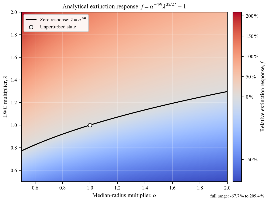
Figure 7 Analytical relative extinction response to r_m multiplier α and LWC multiplier λ. The black curve marks f=0, the open circle marks the unperturbed state, and the diverging colour scale spans the complete calculated range.

5 Application of the algorithm to visibility retrieval

Figures 8 and 9 illustrate the retrieved temporal and spatial evolution of fog microphysical parameters and visibility during a criterion-selected case on 2 March 2025. Influenced by a southern-branch trough, warm and humid southerly airflows advected over the observation site, producing a typical advection sea fog. The fog developed rapidly after 18:00 local standard time (LST) and reached maximum intensity around 21:00 LST. At the radar elevation angle of 2°, fog returns were detectable to a maximum range of approximately 10 km, and the fog-top height exceeded 350 m. Between 18:00 and 24:00 LST, the radar reflectivity factor Z generally decreased with increasing range, indicating a stable fog structure whose density decreased with altitude. During 20:00 to 22:00 LST, numerous range gates with Z exceeding −10 dBZ were observed, with peak values approaching 0 dBZ. As shown in Fig. 8, the polar scan at 20:29 LST reveals that high-Z regions were concentrated to the south and southwest of the observation site, where topographical undulations and man-made structures are distributed. The uneven underlying surface generates turbulence through surface friction, which promotes droplet coalescence and the formation of larger droplets, thereby enhancing Z.

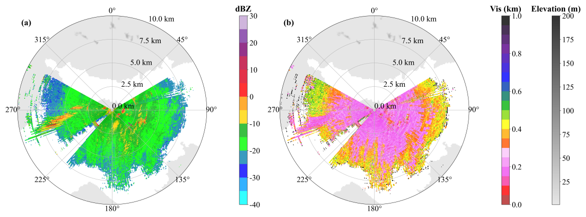
Figure 8 Polar radar scans at 20:29 LST on 2 March 2025: (a) measured radar reflectivity factor (dBZ) and (b) retrieved visibility (km). Range rings are in kilometres, and grey shading gives the displayed elevation context.

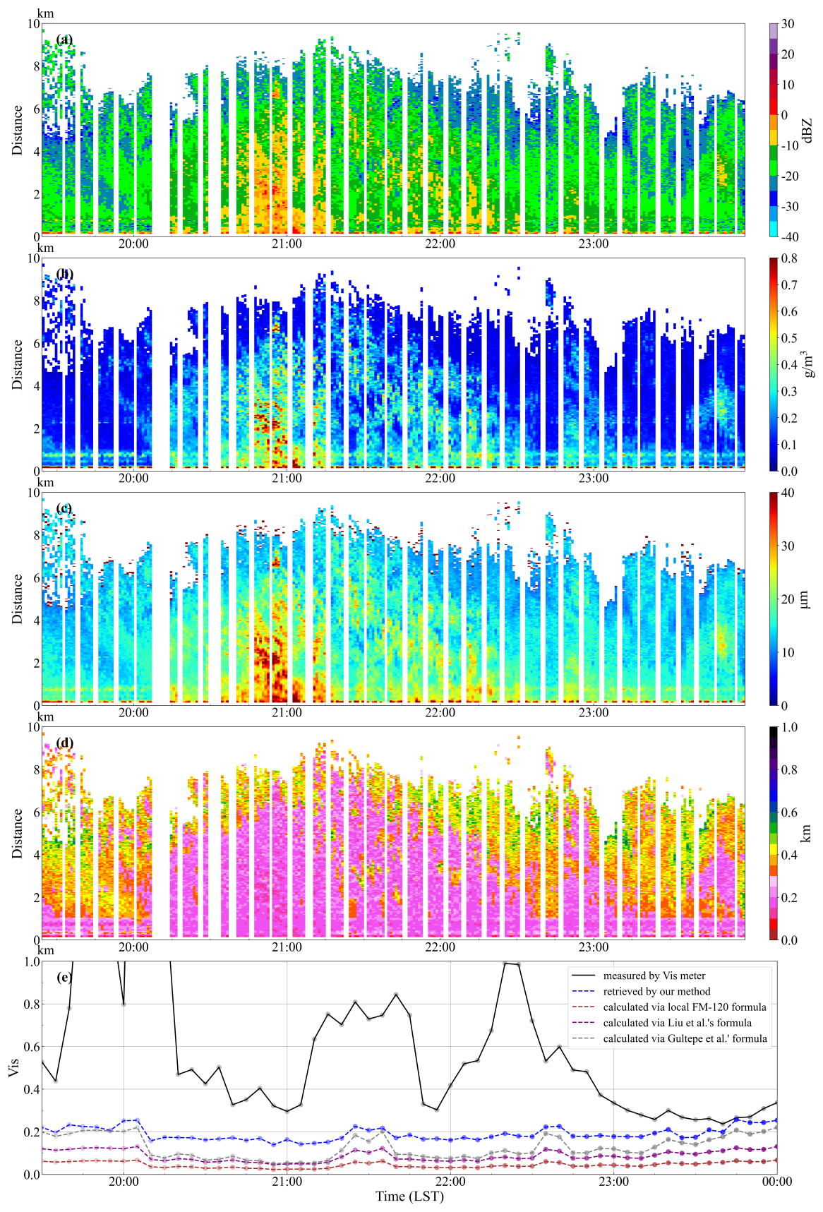
Figure 9 Application to the criterion-selected low-visibility case on 2 March 2025 (Local Standard Time, LST): (a) radar reflectivity (dBZ), (b) retrieved LWC (g m⁻³), (c) retrieved geometric median radius r_m (µm), and (d) retrieved visibility (km), shown versus LST and range (km); (e) visibility time series (km) comparing the DNQ3 visibility meter, the present retrieval, the local site-specific FM-120 relation, Liu et al. (2019, Eq. 7), and Gultepe et al. (2009, Fig. 10b), with provenance and equations in Table 1.

To assess retrieval performance, the present method was cross-validated against DNQ3 forward-scattering visibility-meter observations and three direct empirical visibility–reflectivity relations (Table 1). Near-range radar data are susceptible to ground-clutter contamination, and the minimum detection range is approximately 150 m; the comparison point was therefore selected at 300 m along the 150° azimuth, where the temporal variation correlated most closely with DNQ3. A systematic height difference exists between the DNQ3 sensor at 1.5  m a.g.l. and the radar detection altitude of approximately 30 m at this range, arising from the 25 m antenna height and the beam elevation geometry. Notably, at 21:30 and 22:30 LST, DNQ3 visibility increased markedly while the radar retrievals did not show a corresponding rise. The intense radar echo around 21:00 LST indicates vigorous fog processes that induced droplet sedimentation; the resulting larger particles reduced the total droplet number concentration and raised near-surface visibility as measured by DNQ3 at 1.5 m, while the radar, sampling at a higher altitude, was less affected. Furthermore, the present retrieval is based on backscatter whereas DNQ3 exploits forward scattering, so inherent principle-related differences also contribute to the observed discrepancies. Comparison of FM-120-derived Mie-scattering visibility against DNQ3 shows the same tendency: the retrieval is lower than DNQ3 during the early-to-mature fog stage and converges during dissipation. It should also be noted that the FM-120 fog spectrometer has a limited observation range for large droplets, so variations in the median radius cannot be fully captured in the fitting process when large fog droplets are present, leading to larger biases in the fitted median-radius values.

Table 1 Direct visibility–reflectivity relations used in Figs. 9e and 10.

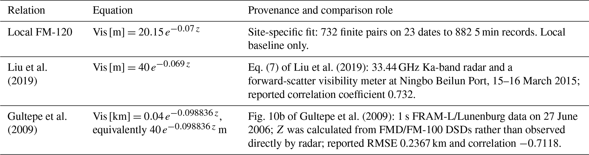
The local and Liu et al. (2019) prefactors are 0.02015 and 0.040 km, respectively, for the kilometre axes in Figs. 9e and 10. The local relation was derived by weighted nonlinear least-squares fitting of 5 min aggregated visibility–reflectivity pairs from FM-120 DSD observations, with elevated weight applied to the low-reflectivity regime where visibility sensitivity is highest (Table 1). Because the radar sampling volume and the DNQ3 point measurement differ in geometry and representativeness, and DNQ3 data also conditioned the event selection and range-gate matching, the comparison in Fig. 10 assesses local consistency and reasonable range rather than ranking methods.

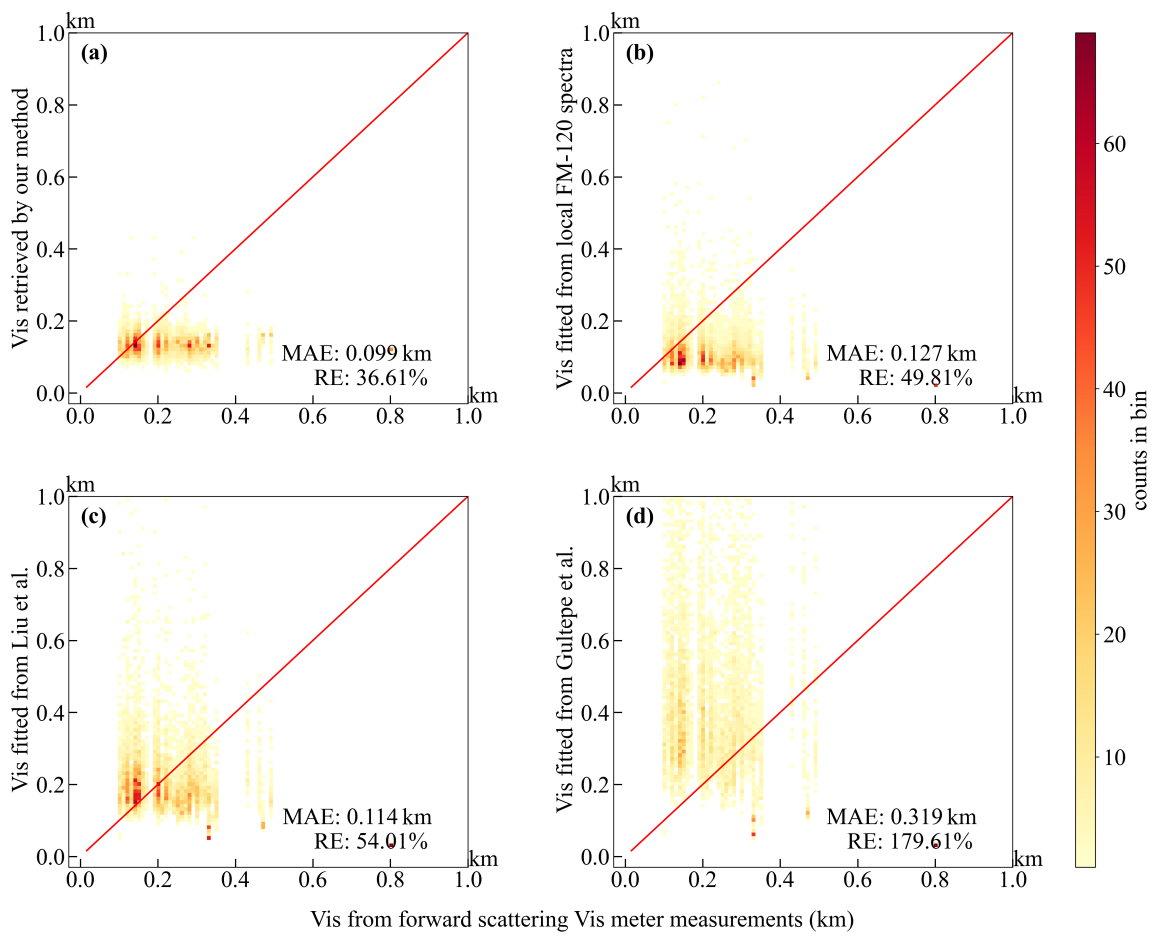
Figure 10 DNQ3-conditioned local-consistency comparison: DNQ3 visibility-meter observations versus (a) the present retrieval, (b) the local site-specific FM-120 relation, (c) Liu et al. (2019, Eq. 7), and (d) Gultepe et al. (2009, Fig. 10b); equations and provenance are given in Table 1. Axes are in kilometres; red lines show 1:1 agreement and colour denotes counts per displayed bin.

Taken together, Figs. 8–10 present the algorithm outputs used only for a DNQ3-conditioned reasonable-range and local-consistency comparison in the criterion-selected coastal low-visibility cases. Owing to systematic differences between the radar sampling volume and the DNQ3 point measurement, as well as the conditioning of event selection and range-gate matching on DNQ3 data, this evaluation reflects local consistency under conditioned samples rather than independent retrieval validation. A stricter quantitative evaluation requires more completely collocated observations over additional fog regimes and explicit characterization of inter-instrument systematic differences.

6 Conclusions

This study presents a physically constrained, observation-calibrated visibility retrieval algorithm for single-wavelength Ka-band millimeter-wave cloud radar. DSD moment analysis confirms that single-wavelength reflectivity cannot uniquely determine both droplet number concentration and geometric median radius, motivating the introduction of two intermediate microphysical constraints. The first is a segment-wise mass-absorption LWC power law that operates on contiguous 4–10-gate segments with reflectivity-dependent starting vectors, a strong-branch retry, and branch-specific attenuation accumulation. The second is an extinction-oriented radius–reflectivity parameterization calibrated against same-source FM-120 DSD observations, enabling closed-form calculation of the extinction coefficient and hence visibility. Compared with purely empirical visibility–reflectivity relations, the proposed method provides clearer physical underpinnings and better internal self-consistency. The main findings are summarized as follows.

During algorithm development, the dominant error sources are identified as the constant extinction efficiency (Q_ext=2) approximation and the single-lognormal DSD assumption. Multi-year FM-120 observations reveal high morphological diversity in coastal fog spectra: broad-unimodal spectra dominate, whereas bimodal spectra become increasingly prevalent below 200 m visibility. Both LWC and Z exhibit strong discriminability across fog-intensity regimes, and this contrast is exploited to optimize the mass-absorption retrieval framework following Ge et al. (2023).

The single-lognormal closure introduces inherent uncertainty into the radius–reflectivity relation. The extinction-oriented parameterization mitigates systematic extinction retrieval errors without additional observational inputs, with more pronounced improvement in dense fog characterized by relatively high reflectivity, achieving a mean absolute fractional extinction error of 9.37 % on the development dataset. Both intermediate quantities (r_m and LWC) carry retrieval uncertainties, and LWC perturbations exert a stronger influence on the final visibility estimate than median-radius perturbations. Within the perturbation range of 0.50–2.00 times the baseline values, the relative change in extinction spans from −67.7 % to +209.4 %. Nevertheless, the covariation of r_m and LWC can partly compensate for individual errors, as reflected in the analytical sensitivity response.

Evaluation on ten criterion-selected spring low-visibility fog events shows that the near-surface visibility retrieved by the proposed method achieves the lowest error statistics among the four compared relations, with a mean absolute error (MAE) of 0.092 km and a relative error (RE) of 42.86 %, followed by the local site-specific FM-120 relation (MAE = 0.123 km, RE = 50.53 %) and Liu et al. (2019) (MAE = 0.160 km, RE = 85.30 %), whereas the Gultepe et al. (2009) relation departs most strongly (MAE = 0.533 km, RE = 310.63 %). The present retrieval, the local FM-120 relation, and Liu et al. (2019) yield broadly comparable visibility ranges, consistent with their shared origin in Fujian Province coastal-fog observations, while the larger departure of Gultepe et al. (2009) reflects regional and latitudinal differences in fog microphysics. However, owing to the spatial mismatch between the radar sampling volume and the ground point measurement, as well as the conditioning of event selection and range-gate matching on DNQ3 data, this evaluation reflects local consistency under conditioned samples rather than independent retrieval validation.

Several limitations of this study must be acknowledged. First, independent in situ LWC measurements and standardized hydrometeor phase data are unavailable, so the retrieved microphysical parameters cannot be validated against reference truth. Second, near-range retrieval results may still be affected by residual ground clutter, as the full quantitative performance of the clutter-filtering algorithm cannot be completely verified. Third, the study samples are limited to spring warm fog at a single southeast coastal site, so the generalizability of the algorithm to other fog types (e.g., radiation fog, orographic fog) and other climate regions remains to be tested.

Future work will pursue three directions. First, dual-wavelength cloud radar observations will be incorporated to further constrain LWC retrieval using differential attenuation characteristics, reducing the non-uniqueness of microphysical parameter estimation. Second, a multi-source synergistic visibility retrieval scheme will be developed by combining lidar, microwave radiometer, and fog-spectrometer observations to add phase identification, vertical structure, and microphysical constraints. Third, observational samples from diverse climate zones and fog types will be accumulated to improve parameterization robustness and generalizability, and to carry out targeted error evaluation for transportation and civil aviation operational applications.