Performance validation of the GHGSat methane constellation via controlled releases

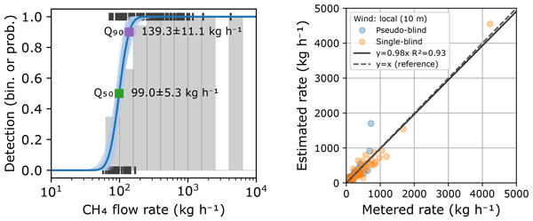
Satellite remote sensing has become an important tool for detecting, quantifying, and attributing methane emissions, yet a rigorous, condition-dependent characterization of point-source imager performance validated against controlled releases with known emission rates remains limited, despite being essential to support its use in regulatory and voluntary reporting frameworks. We present a comprehensive performance assessment of the GHGSat constellation of high-resolution methane-imaging satellites based on a multi-campaign controlled release dataset spanning 2021 to 2026 that combines self-organized campaigns with independent third-party experiments. We develop a probabilistic, environmental conditions-dependent detection model in which the probability of detection depends on the plume signal to noise ratio (SNR), which is in turn a function of emission rate, wind speed, retrieval noise, and spatial resolution. Comparing model variants over subsets of these predictors, we find that emission rate, wind speed, and retrieval noise are the dominant drivers of detection, while spatial resolution improves the fit only when combined with the others. We find that an SNR of 1.72 ± 0.39 is required to achieve a 50 % probability of detection, which translates to a detection limit Q₅₀ = 99.0 ± 5.3 kg h⁻¹ in median environmental conditions encountered in controlled releases (3 m s⁻¹ wind speed, 7 mmol m⁻² column density noise, 27 m resolution). Evaluated over global observing conditions, the same model gives a median Q₅₀= 159.7 kg h⁻¹. The estimated Q₅₀ is shown to converge stably as data accumulate and to remain consistent when blind validation samples are added to self-organized releases. Quantification accuracy is evaluated through parity analysis of estimated versus metered emission rates, yielding an ordinary least squares slope of 0.93 ± 0.03 and R² of 0.92 using reported model winds, improving to 0.98 ± 0.03 and R²= 0.93 with a co-located anemometer wind adjusted to a 10 m reference height. A comparison of emission rate estimates based on ERA5, IFS, and HRRR winds shows that quantification accuracy metrics derived from this dataset were largely insensitive to the choice of operationally available wind product, with a residual underestimation at low emission rates that correlates with wind model spatial resolution. We further demonstrate a bias correction combining a local concentration background correction with an empirically recalibrated effective wind speed, which recovers the low-rate sources that were previously underestimated and removes most of the residual bias without degrading accuracy at higher emission rates. These results establish a transparent, statistically grounded baseline for the GHGSat constellation's detection and quantification performance and provide a methodological framework that can be extended as additional controlled-release data become available.

1 Introduction

Methane (CH₄) is the second most important anthropogenic contributor to global warming after carbon dioxide, responsible for approximately 20 %–30 % of the total anthropogenic increase in radiative forcing since pre-industrial times (IPCC, 2021; Saunois et al., 2025). Its relatively short mean atmospheric lifespan (∼ 10 years) and strong global warming potential (80 times that of CO₂ over a 20-year period) make near-term reductions in methane emissions a critical lever for limiting the pace of climate change (IPCC, 2021, 2022). A growing body of sector-specific regulations and voluntary frameworks reinforces this commitment, with industrial actors across the energy and waste sectors increasingly required – or choosing – to monitor, report, and mitigate their methane footprints.

Satellite-borne remote sensing has become an important tool for methane monitoring, providing spatially extensive observations that complement ground-based, airborne, and facility-level measurement approaches. By detecting, quantifying, and localizing emissions over large areas and repeated observation campaigns, satellite observations can support emissions reporting and inventory development, advance scientific understanding of emission processes and magnitudes, and can inform targeted mitigation actions by pinpointing large, previously unidentified sources (Jacob et al., 2016). GHGSat was among the first organizations to demonstrate high-resolution methane sensing from space. Its first demonstration satellite, GHGSat-D “Claire”, was launched in June 2016, establishing the feasibility of facility-scale methane detection and quantification from orbit (Jervis et al., 2021). Since then, GHGSat has built and deployed a commercial constellation which currently comprises 16 satellites in low Earth orbit.

Methane point-source imagers – including GHGSat, other purpose-built instruments such as Tanager, and public satellites not originally intended for methane measurement such as EMIT, EnMAP, PRISMA, Sentinel-2, and Landsat-8 – are validated and compared on two end-user metrics: the probability of detection (PoD), which characterizes the ability of a system to detect emissions in a noisy background; and the quantification accuracy, which characterizes how faithfully the estimated emission rate reflects the true source rate. Both metrics are assessed through controlled releases, in which a precisely metered flow of methane is emitted at a known location and time while the sensor system attempts to detect and quantify the release. Because the source rate and observing geometry are independently known, controlled releases provide one of the most direct means of evaluating methane-imaging performance (Thorpe et al., 2016; Bell et al., 2022; Sherwin et al., 2023, 2024; El Abbadi et al., 2024; Chen et al., 2024; McManemin et al., 2026; Reuland et al., 2026).

This article presents an analysis of the GHGSat constellation performance based on a multi-campaign controlled release dataset spanning 2021 to 2026, combining both self-organized and third-party campaigns. We introduce a probabilistic, environmental conditions-dependent model based on the mass-balance heuristic from Jacob et al. (2016) to describe the detection performance of the GHGSat constellation as a function of the ratio of source rate (q) over retrieval noise (n), spatial resolution, and wind speed (u) with a linear offset parameter (u₀). Quantification accuracy is evaluated in parallel through a parity analysis of the estimated emission rates, including two approaches for bias correction and the influence of the wind product used. The article closes with a discussion of how these results transfer to operational monitoring beyond the controlled-release setting.

2 Controlled release methods and dataset

The results and analyses presented in this article draw on a compilation of controlled-release campaigns, summarized in Table 1. Measurement data from all methane-sensing satellites that use the current version of the GHGSat spectrometer (GHGSat-C2 and above) are included. Each acquisition is classified as one of four outcomes relative to the known release state: true positives (TP, releases correctly detected), false negatives (FN, releases missed), true negatives (TN, correctly reporting no emission when none was released), and false positives (FP, an emission reported when none was released). Table 1 reports the total number of samples in each classification per campaign and the total for the complete dataset.

Table 1 Summary of controlled release campaigns for the GHGSat constellation.

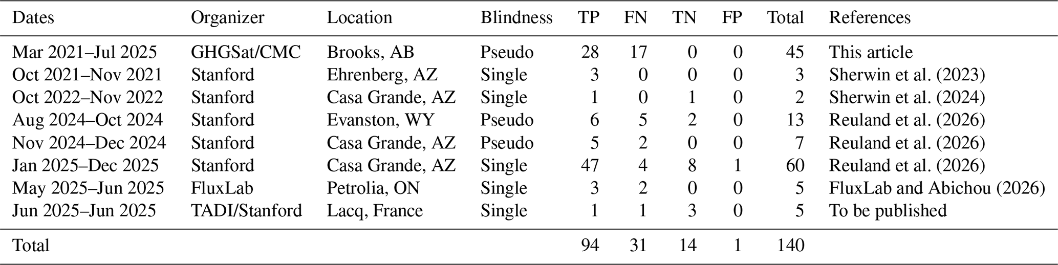
We distinguish two types of experiments: single-blind and pseudo-blind. In a single-blind experiment, an independent third party organizes the campaign and performs ground operations and reference measurements; the measurement provider (GHGSat) is kept unaware of the emission rate and the presence or absence of a release. GHGSat has participated in several such blind studies, including the campaigns organized by Stanford University (Sherwin et al., 2023, 2024; Reuland et al., 2026), FluxLab (Bourlon et al., 2026; FluxLab and Abichou, 2026), and the TotalEnergies Anomalies Detection Initiatives (McManemin et al., 2026). Before the large-scale ramp-up of blind samples in 2024–2025, the need for self-validation motivated a series of campaigns between 2021 and 2025, organized in partnership with Carbon Management Canada (CMC) and the University of Calgary at the Atmospheric Fugitive Emission (AFE) test facility near Brooks, Alberta (Blackmore et al., 2025; CMC, 2025; Wigle et al., 2024). These campaigns are not strictly blind – GHGSat co-organized them and participated in ground operations – but for performance analysis the measurements were processed in a pseudo-blind manner, using the same inspection and quantification methods as in a blind experiment or routine operations. The setup and methodology for those releases are described in Sect. S1 in the Supplement. We also label as pseudo-blind the “phase 0” of the Stanford study at the Wyoming and Arizona sites, since results from this preparatory phase were openly shared between the organizers and participating teams.

Figure 1 shows one representative observation from each of the six controlled-release sites included in this study. The upper row, panels (a–f), shows the retrieved albedo, which provides the surface context of each site. The lower row, panels (g–l), shows the corresponding retrieved methane column density enhancement together with the plume mask used for quantification (dotted white outline). Each methane panel is annotated with the metered emission rate q and the local wind speed u averaged over the 5 min window preceding the observation, and each albedo panel with the site and date of the acquisition. The six sites span a range of surface types: the open prairie of the Brooks facility, the arid and highly reflective terrain of the Arizona and Wyoming sites, and the more vegetated and structurally cluttered Petrolia and Lacq sites.

Two of the panels are shown together to illustrate the conditions-dependence of detection. Panel (k) is a false negative: no plume could be identified at the release location at a metered rate of 79 kg h⁻¹, in a wind of 1.9 m s⁻¹. Panel (l) is a true positive at a comparable metered rate of 72 kg h⁻¹, but in a lower wind of 0.6 m s⁻¹ and over a substantially less noisy CH₄ background. The pair illustrates the central premise of the detection model developed in Sect. 3: the emission rate alone does not determine whether a release is detected, and the same rate can fall on either side of the detection threshold depending on the wind speed and the retrieval noise of the scene.

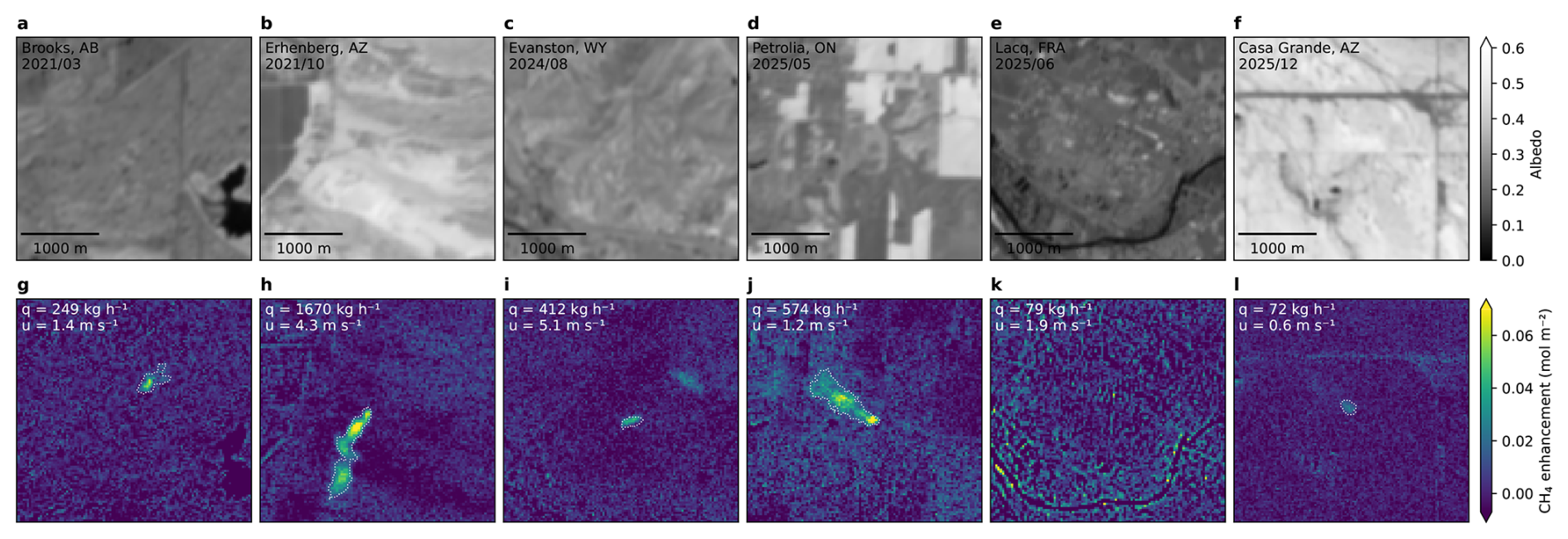
Figure 1 Example observations from each of the six controlled-release sites. (a–f) Retrieved albedo, labelled with the site and acquisition date. (g–l) Corresponding retrieved methane column density enhancement and plume mask boundary (dotted white line), labelled with the metered emission rate q and the local wind speed u. Panel (k) is a false negative and panel (l) a true positive at a comparable metered rate; the two differ in wind speed and retrieval noise.

2.1 Satellite data acquisition

GHGSat satellites measure the methane concentration in the atmosphere based on the general principle of absorption spectroscopy. The main optical payload is a wide-angle Fabry–Pérot (WAF-P) interferometer, which provides spectrally resolved measurements of backscattered sunlight in the shortwave infrared (SWIR), targeting methane-specific absorption lines around 1.6 µm (Jervis et al., 2021).

GHGSat satellites operate in target mode, collecting multiple partially overlapping camera frames over a 20 s acquisition window. During that time, the field of view is translated along the direction of satellite motion at a rate much slower than the orbital velocity, allowing optical signal to be collected over each ground point for a longer interval than nadir-pointing would permit. Target-pointing maneuvers and acquisition settings during controlled releases matched those of standard commercial operations.

Unlike global imagers, which survey the whole Earth periodically, GHGSat observations are tasked in advance for specific targets. Controlled-release opportunities were therefore coordinated between GHGSat mission planning and the partner ground team, balancing upcoming orbital overpasses, weather forecasts, commercial scheduling constraints, and the availability of ground staff at the release facility.

After each observation, the raw level 0 (L0) data are downlinked and processed by GHGSat's proprietary toolchain to produce the deliverable L2 products (spatially resolved albedo, methane enhancement, and uncertainty) and L4 products (emission identification and quantification).

2.2 Source identification and quantification

Emission plumes are identified based on methane enhancement, its associated uncertainty, and the albedo, in accordance with the GHGSat standard operating procedures. To distinguish true methane enhancements from noise and artifacts, the spatial structure of the plume (general morphology, alignment with the wind direction) is assessed, and the enhancement should not correlate with features present in the albedo layer. Inspection of the albedo field and publicly available imagery of the surveyed sites provides additional contextual information on the presence or absence of potential methane-emitting sources.

Once an emission plume is identified, the methane emission rate is estimated using the integrated mass enhancement (IME) method (Varon et al., 2018). We express the IME as the sum of column density enhancements over the visible extent of the plume:

$$\begin{array}{}\text{(1)}& \mathrm{IME}=\sum _{x,y\in M_{\mathrm{p}}}\mathrm{\Omega }\left(x,y\right)A_{\mathrm{pix}},\end{array}$$

where the sum is carried over pixels that are included in a plume mask M_p in which the enhancements are visible above the noise level, and A_pix is the area of a retrieval pixel in ground coordinates. The IME quantifies the local accumulation of methane and is driven by two factors: the actual emission rate q, and the rate at which the methane dissipates in the surrounding atmosphere, which in turn is driven by wind speed u. Those quantities are related mathematically through the equation

$$\begin{array}{}\text{(2)}& q={\displaystyle \frac{U_{\mathrm{eff}}\left(u_{\mathrm{10}}\right)}{L_{\mathrm{eff}}}}\mathrm{IME},\end{array}$$

where q is the emission rate, U_eff is the effective wind speed, and $L_{\mathrm{eff}}=\sqrt{A}$ is an effective plume length defined as the square root of the area of the plume mask. The effective wind speed is expressed as a function of the wind speed at 10 m above ground u₁₀, a quantity available from most global weather models, through an empirical relationship obtained from a large ensemble of simulations (Maasakkers et al., 2022; Varon et al., 2018):

$$\begin{array}{}\text{(3)}& U_{\mathrm{eff}}=\mathrm{0.34}{u}_{\mathrm{10}}+\mathrm{0.42}.\end{array}$$

Plume masks are generated in four steps: Gaussian filtering for noise suppression, thresholding against the local noise level, rejecting pixels that are not connected to the plume origin, and connecting disjoint “puffs” using binary dilation. The method is semi-automated: it provides reasonable default parameters at each step but allows GHGSat analysts to adjust them so that only real enhancements – not albedo-correlated artifacts – are included in the mask.

3 Detection performance

3.1 Conditions-dependent probability of detection

The detection capability of a remote-sensing system is commonly characterized by its probability of detection (PoD). High-level performance metrics such as Q₅₀ and Q₉₀ – detection limits at a probability of 50 % or 90 % respectively – can be useful for comparing systems. However, advanced quantitative applications such as building measurement-informed emission inventories (Chen et al., 2022; Johnson et al., 2023; Donahue et al., 2026; Jervis et al., 2026b) require a more rigorous description that incorporates two key features (McKeever and Jervis, 2025). First, the detection limit is conditions-dependent, varying with both environmental and operational factors. Second, detection is probabilistic: small emissions have a lower probability of being detected than large ones, but the transition is smooth rather than a hard cutoff.

Here we use a probabilistic formalism following (Conrad et al., 2023; Ayasse et al., 2024; Thorpe et al., 2024; Manninen et al., 2026), where we express the probability of detection as

$$\begin{array}{}\text{(4)}& \mathrm{PoD}=P\left(Z\left(\mathit{X};\mathit{\varphi }\right);\mathit{\theta }\right),\end{array}$$

which is the composition of two functions commonly referred to as the predictor function Z(X;ϕ) and the inverse-link probability function P(Z;θ). Conceptually, Z(X;ϕ) models how a vector X of observation-specific, environmental and operational variables (emission rate, wind speed, etc.) affect how detectable an emission is at processing level 2. On the other hand, the function P(Z;θ) smoothly maps the predictor to a normalized probability. Its parameters θ characterize the “inspection” process (level 4), and may be affected by the type of processing (automated vs. manual) and the quality of prior information (presence or absence of known potential emitter). The vectors ϕ and θ are model parameters which can be obtained by fitting to binary results of controlled releases, maximizing the likelihood ℒ – or equivalently minimizing the negative log-likelihood (NLL) – of a sequence of independent Bernoulli trials:

$$\begin{array}{}\text{(5)}& \mathrm{NLL}=-\ln \mathcal{L}=-\sum _{i\in \left\{\mathrm{TP},\mathrm{FN}\right\}}{d}_i\ln p_i+\left(\mathrm{1}-d_i\right)\ln \left(\mathrm{1}-p_i\right),\end{array}$$

where the summation is carried over the true positive (TP) and false negative (FN) controlled release results, d_i is the binary detection result, and $p_i=P\left(Z\left({\mathit{X}}_i;\mathit{\varphi }\right);\mathit{\theta }\right)$ is the probability of detection model evaluated at the set of environmental parameters for each specific release X_i. The choice of appropriate parameters and functional forms for the predictor and link functions requires consideration and is examined in the following sections.

As a note, the function P(Z;θ) used in this article represents the conditional probability of detection, given the existence of a true emission $\mathcal{P}\left(d=\mathrm{1}|q>\mathrm{0}\right)$. This is distinct from the marginal probability of a positive or negative detection outcome

$$\begin{array}{}\text{(6)}& \mathcal{P}\left(d\right)=\mathcal{P}\left(d|q>\mathrm{0}\right)\mathcal{P}\left(q>\mathrm{0}\right)+\mathcal{P}\left(d|q=\mathrm{0}\right)\mathcal{P}\left(q=\mathrm{0}\right),\end{array}$$

which includes a second term describing false positive (FP) and true negative (TN) outcomes. The marginal probability is not an intrinsic property of a sensor or observing system, as it depends on the population of emission sources being surveyed via the 𝒫(q>0) and 𝒫(q=0) priors. A complete description of the GHGSat constellation performance would in principle require both the $\mathrm{TP}/\mathrm{FN}$ and $\mathrm{FP}/\mathrm{TN}$ conditional probabilities listed in Eq. (6). However, while the number of samples available allows us to model and parameterize the $\mathrm{TP}/\mathrm{FN}$ case as described in the following sections, the small sample size for FP and TN does not allow a parallel approach, and we limit ourselves to reporting the number of outcomes in Table 1.

3.1.1 Predictor variables

Jacob et al. (2016) introduced a useful heuristic for the detection limit by estimating the peak methane enhancement from a point source in a uniform wind field, and imposing a minimum signal to noise ratio for the detection. With minor changes to the original publication in terms of units and variable rearrangement, this heuristic can be expressed in the following form:

$$\begin{array}{}\text{(7)}& Z={\displaystyle \frac{q}{una}},\end{array}$$

where q is the emission rate (mol s⁻¹), u is the wind speed (m s⁻¹), n is the noise on the measured methane column density (mol m⁻²), a is the spatial resolution of the instrument (m), and Z is a dimensionless quantity representing the signal to noise ratio of the highest plume enhancement, providing a measure of plume “detectability” (Bruno et al., 2024; Manninen et al., 2026).

Importantly, the Jacob heuristic identifies the set of parameters $\mathit{X}=\left\{q,u,n,a\right\}$ upon which the PoD should depend, excluding higher order effects. Other parameters commonly identified as drivers of detection performance – surface albedo, topography, solar and viewing angles, scan panning speed, sensor-to-ground distance, meteorological conditions, atmospheric composition, and camera settings – are intermediate variables that act through either the spatial resolution or the noise. This makes it possible to conceptualize a conditions-dependent model that is simple enough to constrain via controlled-release data, yet broadly applicable across operational conditions (Thorpe et al., 2024).

To assess the relative predictive strength of each variable, our analysis evaluates several subsets of the four core parameters: X={q} (a plain regression as a function of source rate); $\mathit{X}=\left\{q,u\right\}$ (a commonly assumed dependence on $q/u$); other possible 2- and 3-variables subsets; and the full set $\mathit{X}=\left\{q,u,n,a\right\}$.

In this study, the source rate q is defined as the time average of the flow rate reported by the flowmeter q_fm(t), over an integrating window starting T minutes before the observation and ending at the observation time t_obs:

$$\begin{array}{}\text{(8)}& q={\displaystyle \frac{\mathrm{1}}{T}}{\int }_{t_{\mathrm{obs}}-T}^{t_{\mathrm{obs}}}{q}_{\mathrm{fm}}\left(t\right)\mathrm{d}t.\end{array}$$

The wind speed u is obtained by applying the same averaging window to the magnitude of the local wind time series u_lw(t) measured by the anemometer. We used an integrating window length of 5 min, ensuring consistency with published datasets (Sherwin et al., 2023, 2024). Unless stated otherwise, u denotes the wind speed as measured at the anemometer height (z_ane), and this is the quantity used throughout the detection analysis of Sect. 3. Because the effective wind speed used in the IME method is calibrated for an input wind at z_ref= 10 m above ground, the quantification analysis of Sect. 4 additionally considers this wind adjusted to a 10 m reference height, assuming a logarithmic wind profile:

$$\begin{array}{}\text{(9)}& u\left(z_{\mathrm{ref}}\right)=u\left(z_{\mathrm{ane}}\right){\displaystyle \frac{\ln \left(\left(z_{\mathrm{ref}}-d\right)/z_{\mathrm{0}}\right)}{\ln \left(\left(z_{\mathrm{ane}}-d\right)/z_{\mathrm{0}}\right)}},\end{array}$$

where z₀ is the roughness length and d is the zero-plane displacement. Specific values of z_ane, z₀ and d for each campaign are tabulated in Table S1 in the Supplement.

The spatial resolution metric a sets how tightly a plume is imaged: the coarser the resolution, the more the plume signal is diluted within each pixel and the harder it is to distinguish from the background. Formally, we define a as the width of the optical point spread function (PSF) in ground coordinates, scaled to account for the stretching of pixels when a target is viewed away from nadir:

$$\begin{array}{}\text{(10)}& a={\mathit{\sigma }}_{\mathrm{psf}}{\displaystyle \frac{r_{\mathrm{s}}{p}_{\mathrm{pix}}}{f\cos {\mathit{\theta }}_z}},\end{array}$$

where σ_psf is the standard deviation of the optical PSF in pixels, r_s is the slant distance from satellite to ground target, p_pix is the pixel pitch, f is the focal length, and θ_z is the off-nadir viewing angle.

Finally, the retrieval noise n used in the PoD model is an estimate of the standard error of the methane column density, based on the residuals of the retrieval and averaged within a 500 m radius of the release point. This metric of retrieval noise is distinct from alternative definitions based on physical modelling or spatial statistics, and is formally defined in Sect. S3.

3.1.2 Predictor functions

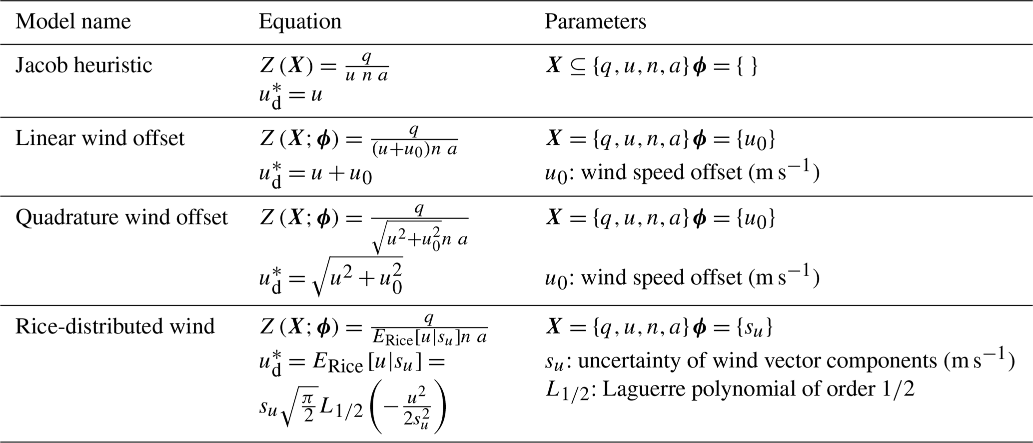
In addition to providing the set of key driving variables, we use the Jacob heuristic as a template to define candidates for the predictor function Z(X;ϕ), which are listed in Table 2 alongside the associated vector of fitted parameters ϕ. The candidates were constructed to address one key limitation of the heuristic, which is that even at an average wind speed of zero, there should still be some amount of methane dissipation due to diffusion and small-scale eddies. This implies that the concentration does not diverge to infinity and the PoD remains less than 1 as u approaches zero. We model this by replacing the plain wind speed u in the heuristic by a function $u_{\mathrm{d}}^{*}\left(u;\mathit{\varphi }\right)$, such that

$$\begin{array}{}\text{(11)}& Z\left(\mathit{X};\mathit{\varphi }\right)={\displaystyle \frac{q}{u_{\mathrm{d}}^{*}\left(u;\mathit{\varphi }\right)na}}.\end{array}$$

We further require the function $u_{\mathrm{d}}^{*}$ to have dimensions of a speed (length over time), which retains the interpretation of Z(X;ϕ) as a dimensionless SNR-like quantity. It follows that $u_{\mathrm{d}}^{*}$ can be interpreted as a “detection” effective wind speed, which is analogous but distinct from the “quantification” effective wind speed of the IME method (Eq. 3).

We evaluate four predictor functions that follow this general form: (1) the ordinary Jacob heuristic, (2) a linear wind offset, which is the simplest extension, (3) a wind offset added in quadrature, which recovers the ordinary heuristic in the limit of high wind speed, and (4) an effective wind function following the mean of a Rice-distributed variable. The Rice model is motivated by representing the estimated 2-D wind vector, $\widehat{\mathit{u}}=\left(\widehat{U},\widehat{V}\right)$, as

$$\begin{array}{}\text{(12)}& \begin{array}{l}\widehat{\mathit{u}}=\mathit{u}\mathbf{+}{\mathit{ϵ}}_u,\end{array}\end{array}$$

where $\mathit{u}=\left(U,V\right)$ is the effective wind vector experienced by the plume and ${\mathit{ϵ}}_u=\left({\mathit{ϵ}}_U,{\mathit{ϵ}}_V\right)$ represents measurement error. Under the assumption that ϵ_U and ϵ_V are independent and normally distributed with standard deviation s_u, the magnitude of the wind vector u follows a Rice distribution with parameters $\mathit{\nu }=\widehat{u}$ and σ=s_u. Its mean is positive even when the nominal wind vector is zero, capturing the expectation that unresolved vector variability produces non-zero effective transport at low reported wind speed.

Previous publications have considered predictors that further generalize the Jacob heuristic by allowing each variable an additive offset and a fitted exponent (Ayasse et al., 2024; Conrad et al., 2023; Thorpe et al., 2024). Enumerating those options exhaustively is not tractable at our sample size: an optional offset and an optional fitted exponent on each of the four variables, combined with the four inverse-link families used in those studies, already defines ${\mathrm{2}}^{\mathrm{8}}\times \mathrm{4}=\mathrm{1024}$ candidates carrying up to 10 fitted parameters, to be constrained by 125 binary outcomes of which only 31 are misses. Selecting the minimum-AICc member of a set of that size would largely reflect sampling noise. We instead restrict the candidate set on physical grounds. Provided that momentum and buoyancy at the release point are too small to change the plume's rise or near-field mixing with emission rate, the concentration enhancement in every pixel is directly proportional to the emission rate. Scaling the emission rate while scaling the noise by the same amount produces an observation that carries the same information about the presence of a plume, so the probability of detection must be unchanged. This is only the case if q and n enter Z through their ratio and without offset. The spatial resolution could in principle carry an offset or exponent, but varies too little to constrain additional parameters, as confirmed by the model comparison in Sect. 3.3. Wind speed is therefore the only variable for which the heuristic is both expected to be incomplete and testable with the available data, and the candidate predictors below differ only in the form of the effective wind speed $u_{\mathrm{d}}^{*}$.

This restriction is consistent with publications that investigated the more general form. The combined model of Thorpe et al. (2024) adopts a predictor with no offset on any variable and fits separate exponents to emission rate and noise, obtaining 1.95 and 2.08 respectively; their ratio of 1.07 indicates that q and n enter through their ratio to within 7 %, close to the linear dependence assumed here. Likewise, none of the optimized predictors reported by Conrad et al. (2023) retains an offset on emission rate. These studies find the heuristic incomplete in the wind term, which is where we concentrate the candidate forms.

Table 2 Predictor functions and associated parameters.

3.1.3 Inverse link functions

The inverse-link functions considered are defined in Table 3. Because the predictor Z(X;ϕ) is a positive, signal-to-noise-like quantity, we restrict the inverse-link functions to cumulative distribution functions with support on the positive real line (Conrad et al., 2023). This choice excludes consideration of models that would predict a non-zero PoD for negative source rates which are unphysical, such as the commonly used logistic and probit inverse link functions. We instead consider their logarithmic counterpart: the log-normal and log-logistic cumulative distribution functions (CDF), as well as the Weibull and Fréchet CDF. Table 3 also expresses alternative parameterizations of the distributions such that they are expressed consistently as an offset and scale, in terms of the logarithm of Z.

Table 3 Inverse-link functions and associated parameters.

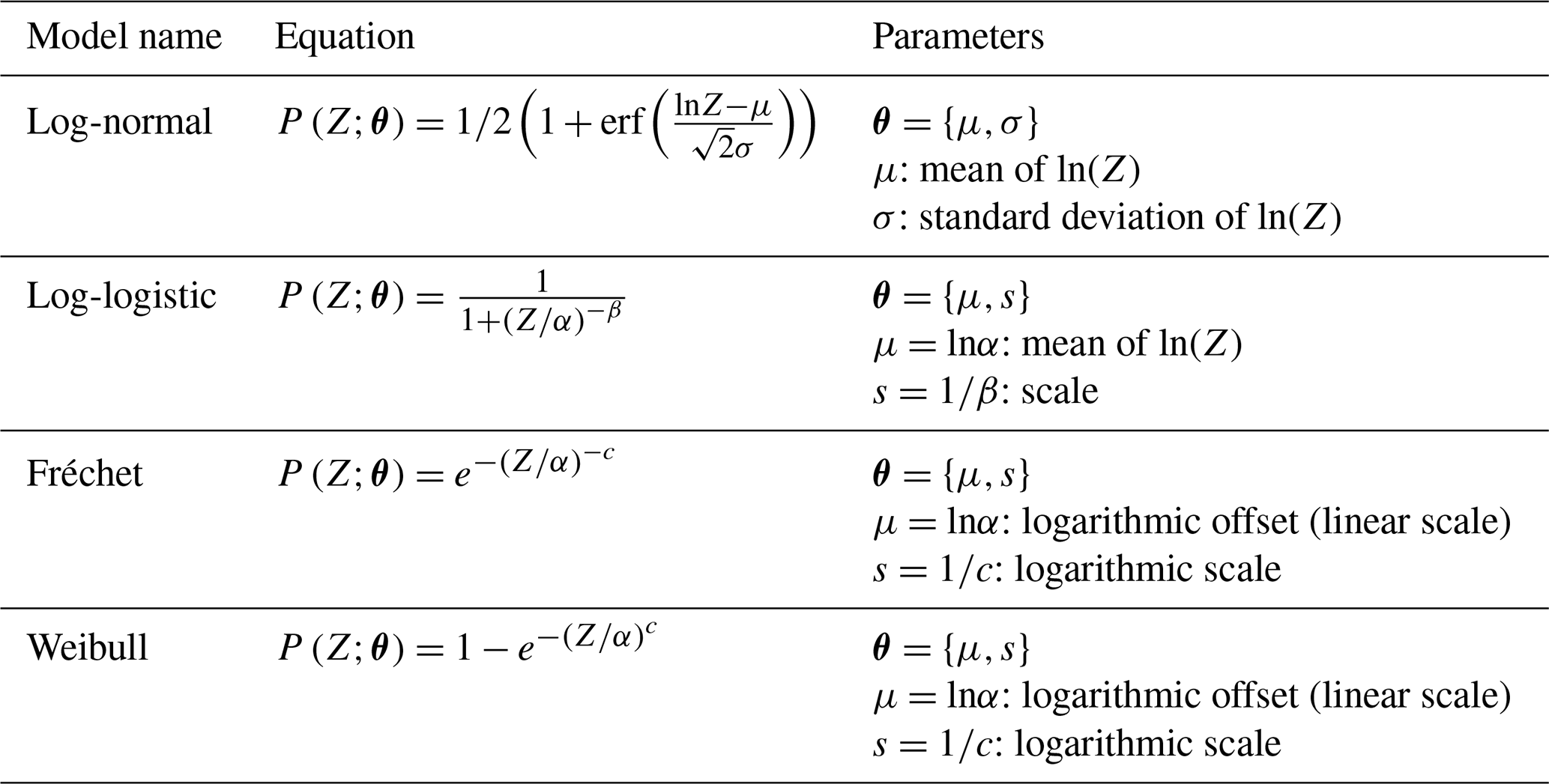
3.2 Experimental results and model regression

The dataset used to analyze detection capability includes 125 samples: 94 TP (detections) and 31 FN (misses), about equally split between single-blind (62) and pseudo-blind (63). Experimental results and fitted regressions are presented graphically in Fig. 2 as functions of the metered methane emission rate (1st column of subplots), the value of the SNR-like predictor function (2nd column), and in a 2-D space with emission rate on the y axis and wind speed on the x axis (3rd column). Due to the large number of possible combinations of link functions, predictor functions, and environmental variable subsets, we selected two models for plotting: the heuristic predictor (first row), and linear wind offset (second row), both using the full set of environmental variables $\left\{q,u,n,a\right\}$ and a log-normal inverse link function. Derived detection limits for an extended list of models are provided in Table 4. Additionally, an analysis comparing the quality of model candidates in terms of the Akaike and Bayesian information criteria will be presented in Sects. 3.3 and S4, supporting the choice of the log-normal linear-offset PoD function as primary model.

Table 4 Detection limits and goodness of fit metrics for the predictor functions and inverse-link functions considered. Values are the results of maximum likelihood optimization and uncertainties are the standard deviation of the bootstrap ensemble. Detection limits are evaluated at u= 3 m s⁻¹, n= 7.0 mmol m⁻², a= 27.0 m.

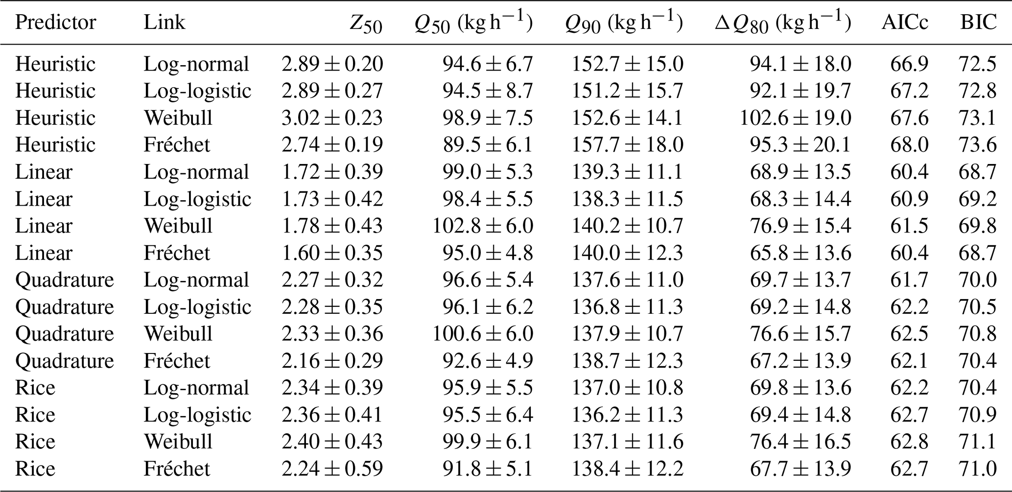
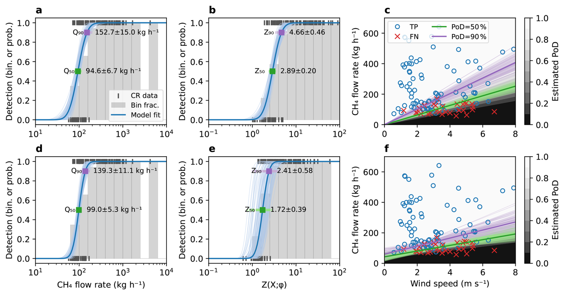
Figure 2 Detection results and fitted probability of detection for two candidate models: (a–c) heuristic, (d–f) linear wind offset. The detections and PoD are plotted as a function of the emission rate (1st column), the SNR predictor value (2nd column), and as a 2D function of emission rate and wind speed (3rd column). Binary results of controlled releases are shown as discrete markers: black vertical ticks, and blue (TP) or red (FN) markers. Histogram bars represent the detection fraction in each corresponding bin. Continuous curves represent the fitted PoD model – thick ones for the maximum likelihood solution and thin ones for the bootstrap uncertainty evaluation. The detection limit at specific PoD of 50 % and 90 % are highlighted in green and purple respectively, with associated text labels providing the maximum likelihood estimate and standard error derived from bootstrapping.

The detection limit at specified PoD corresponds to contours of $P\left(Z\left(\mathit{X};\widehat{\mathit{\varphi }}\right);\widehat{\mathit{\theta }}\right)$ and can be expressed explicitly by solving Eq. (4) for the emission rate:

$$\begin{array}{}\text{(13)}& Q_p=Z_p\left(p;\widehat{\mathit{\mu }},\widehat{\mathit{\sigma }}\right)u_{\mathrm{d}}^{*}\left(u;{\widehat{u}}_{\mathrm{0}}\right)na,\end{array}$$

where Q_p is the emission rate detected with probability p (typically 50 % or 90 %), $Z_p\left(p;\widehat{\mathit{\mu }},\widehat{\mathit{\sigma }}\right)$ is the quantile function of the log-normal SNR predictor, and the circumflex indicates best-fit estimates of the model parameters $\left\{\widehat{\mathit{\mu }},\widehat{\mathit{\sigma }},{\widehat{u}}_{\mathrm{0}}\right\}$. We evaluate the uncertainty of the fitted detection models and all derived parameters using the bootstrapping method. We randomly draw, with replacement, 1000 subsets from the full set of 125 TP and FN controlled release results. For each sample subset and each candidate model (predictor and inverse-link pair), we find the maximum-likelihood solution and retain the associated parameters. This method is used to derive uncertainty bounds on fitted model coefficients ($\mathit{\mu },\mathit{\sigma },u_{\mathrm{0}}$), as well as other derived quantities such as detection limits.

The detection limits Q₅₀ and Q₉₀ are shown in Fig. 2 as square markers (1D subplots) and continuous contour lines (2D subplots of q and u). In particular, specifying PoD = 50 % and median conditions as reference (wind speed u = 3 m s⁻¹, noise n= 7.0 mmol m⁻², and spatial resolution a = 27.0 m), we find the value of Q₅₀ to be highly consistent between the models listed in Table 4, ranging between 89.5 ± 6.1 kg h⁻¹ (heuristic, Fréchet) and 102.8 ± 6.0 kg h⁻¹ (linear wind offset, Weibull). A higher variability between models is observed for Q₉₀, which reflects a difference in transition width. Specifically, models using the heuristic predictor have Q₉₀∼ 150 kg h⁻¹, while other models which include a wind offset cluster around 135–140 kg h⁻¹. This difference is expected if the wind offset parameter (included in all predictors except the heuristic) captures real physics, as any effect unmodeled in the predictor is effectively convolved into the link function.

The detection limit can also be expressed directly in terms of the SNR predictor, with values of Z₅₀ ranging between 1.60 (linear wind offset, Fréchet) and 3.02 (heuristic, Weibull). Note that we observe more jitter of the bootstrap curves when plotting the PoD against Z_p compared to Q_p. This is because the predictor includes a fitted parameter u₀ which has some level of degeneracy with parameters of the inverse-link functions, particularly the offset term μ. In Q space, errors on u₀ are compensated by errors on μ while maintaining a similar derived Q_p, while Z_p does not have that compensation. Because the heuristic model does not have any free predictor function parameters, the jitter on Z_p curves is the same as that of Q_p. Still, in every case, the numerical values are physically realistic considering the interpretation as a SNR, which suggests that a Z_p value around 2 is needed to achieve 50 % PoD, and around 3–4 for 90 % PoD.

3.3 Comparison of detection model variants

The preceding analysis used representative model configurations to illustrate the estimated probability-of-detection behaviour. Here, we expand the analysis to compare alternative choices of predictor variables, predictor functions, and inverse-link functions. We first examine the impact of the driving variables $\left\{q,u,n,a\right\}$ in Fig. 3a–d by varying the subset of variables while fixing the predictor and inverse-link functions to heuristic and log-normal, respectively. The second row of subfigures, Fig. 3e–h, examines all 16 combinations of the four predictor functions and the four inverse-link functions. Fitted parameters and goodness-of-fit metrics for every model variant shown here, including the variable subsets, are tabulated in supplementary Tables S2 and S3. For each case we evaluate Q₅₀ to provide an indication of its consistency and robustness to choice of model, as well as the corresponding transition width ΔQ₈₀=Q₉₀–Q₁₀. Following (Conrad et al., 2023; Thorpe et al., 2024), we use the Akaike information criterion with small-sample correction (AICc) as a metric of fit quality that penalizes overfitting due to excessive parametrization:

$$\begin{array}{}\text{(14)}& \mathrm{AICc}=-\mathrm{2}\ln \widehat{\mathcal{L}}+\mathrm{2}k+{\displaystyle \frac{\mathrm{2}k\left(k+\mathrm{1}\right)}{N-k-\mathrm{1}}},\end{array}$$

where k is the number of fitted model parameters, N is the number of samples, and $\widehat{\mathcal{L}}$ is the value of the likelihood function at the solution (maximum likelihood). We also compute the Bayesian information criterion (BIC):

$$\begin{array}{}\text{(15)}& \mathrm{BIC}=-\mathrm{2}\ln \widehat{\mathcal{L}}+k\ln N,\end{array}$$

as an alternative measure of goodness of fit.

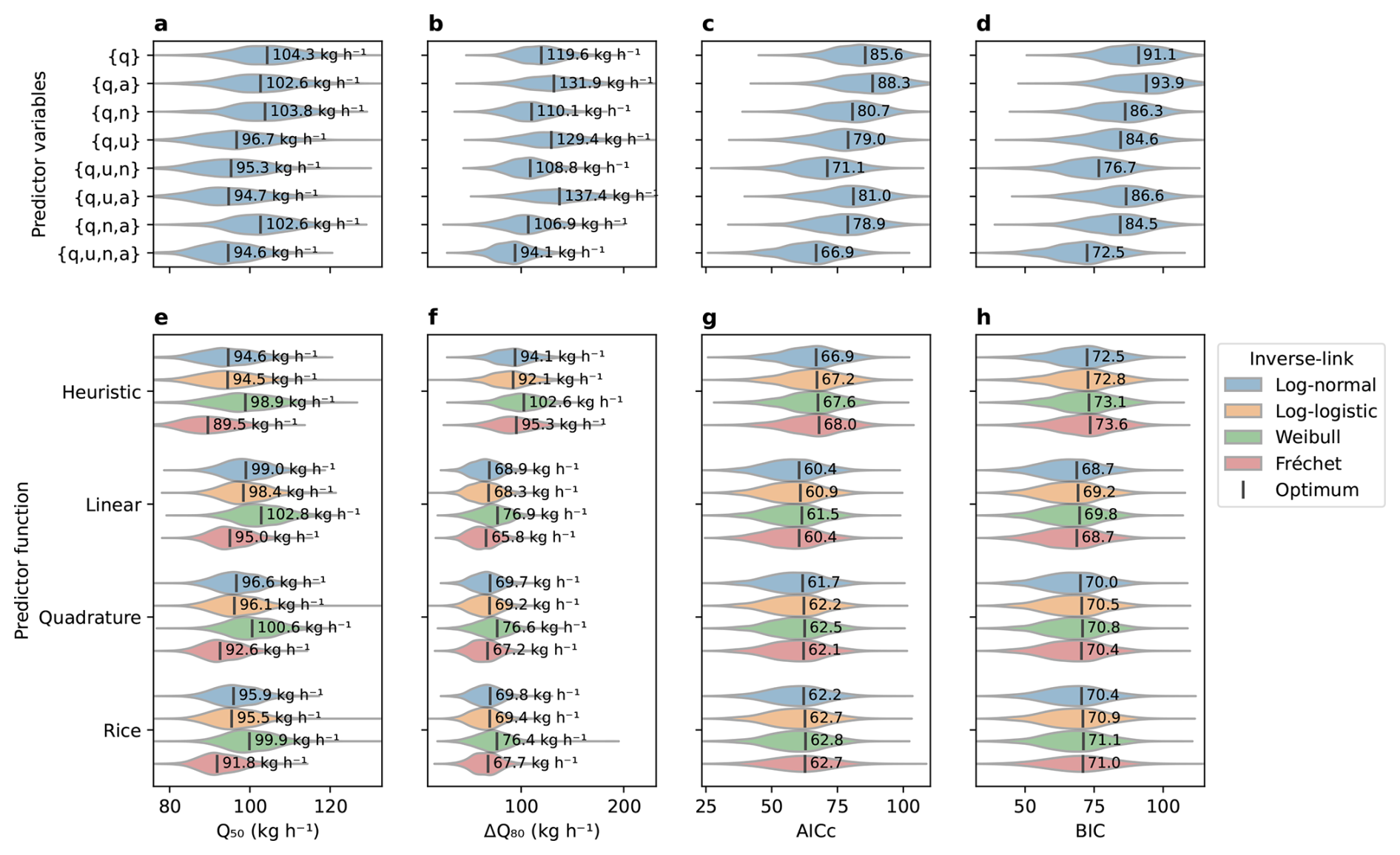
Figure 3 Evaluation and comparison of detection model candidates in terms of (a, e) 50 % detection limit, (b, f) 10 % to 90 % transition width, (c, g) Akaike information criterion, and (d, h) Bayesian information criterion. Top panels (a–d) compare subsets of the driving variables {q, u, n, a} with the predictor and link functions set to Jacob heuristic and log-normal. Bottom panels (e–h) compare all 16 combinations of the four predictor functions (grouped along the y axis) and the four inverse-link functions (log-normal in blue, log-logistic in orange, Weibull in green, Fréchet in red), using the full set of driving variables. Values for the maximum likelihood solution using all samples are labelled textually and noted by a vertical bar, while coloured envelopes represent the distribution of values across the 1000 bootstrap subsets.

Comparing choices of predictor variables, we observe clear variability in model quality, the best models (lowest AICc and BIC) being ones that use all four parameters. Examining the 2- and 3-variables subsets provide interesting insights to their relative influence: there is a clear reduction of AICc and BIC when adding the wind speed (u) or noise (n). Adding spatial resolution (a) by itself does not help as the {q,a}, $\left\{q,n,a\right\}$ and $\left\{q,u,a\right\}$ combinations perform worse than their resolution-free counterparts. However, including the resolution along with the other variables (such as $\mathit{\{}q,u,n,a\mathit{\}}$ vs. $\mathit{\{}q,u,n\mathit{\}}$) improves the model quality, supporting that a should be included in the PoD model. Overall, our analysis of parameters suggests that over the range of operational conditions, q, u and n are the main drivers, while resolution varies little across nominal operating conditions and thus has a less pronounced effect.

Examining the various combinations of predictor and inverse-link functions in Fig. 3e–h, we first note that all of these models perform similarly, with differences between them that fall within the bootstrap uncertainty ranges. Had the analysis been repeated with a somewhat different collection of releases, the models could well have appeared in a different order. We expect the ranking to become better constrained as more releases are added in the coming years. One conclusion is that the plain Jacob heuristic has the highest transition width, AICc, and BIC, supporting the introduction of a wind offset parameter in one form or another. This conclusion can be further assessed by a likelihood-ratio test against the Jacob heuristic (null hypothesis). For the linear model, the test statistic $\mathrm{\Lambda }=\mathrm{2}\left(\ln {\mathcal{L}}_{\mathrm{lin}}-\ln {\mathcal{L}}_{\mathrm{heur}}\right)=\mathrm{8.58}$, evaluated against a χ² distribution with one degree of freedom, yields p=0.003, meaning the improvement in fit is larger than the addition of one free parameter alone would produce. Of the three remaining predictor forms, the linear wind offset results in the lowest information scores, albeit by a small margin compared with quadrature and Rice models. Regarding the choice of inverse-link function, the four candidates fall within 1.1 AICc units of one another at fixed predictor, so the data do not meaningfully discriminate between them. The log-normal link is the best-scoring of the four for the heuristic, quadrature and Rice predictors, and is tied with the Fréchet link for the linear predictor (AICc = 60.4 and BIC = 68.7 for both). The links differ more visibly in the derived detection limits than in the information criteria: at fixed predictor the Fréchet link systematically returns the lowest Q₅₀ and the Weibull link the highest, with the log-normal and log-logistic falling between them and within 1 kg h⁻¹ of each other.

Based on those results, we adopt the log-normal inverse-link function with the linear wind offset predictor, driven by all four variables ($q,u,n,a$), as the primary model for the remainder of this paper. While the information criteria do not discriminate between the log-normal and Fréchet links with the linear predictor, we prefer the log-normal because predictor Z is formed as a product and ratio of positive quantities, each carrying its uncertainty, so a log-normal is the expected distribution. The Fréchet distribution, by contrast, is an extreme-value law applicable to the maxima rather than products. We highlight that the detection limits and transition widths derived from various models in Fig. 3e, f are highly consistent, supporting the robustness of derived performance metrics to the choice of model.

3.4 Convergence and applicability of the detection performance

The analysis presented in Fig. 4 examines the evolution and applicability of the detection model between 2021 and 2026 as the GHGSat constellation grew with new instruments, as the data processing toolchain was upgraded, and as more single-blind samples from the Stanford study became available. The total number of controlled release events prior to a given date is shown in Fig. 4a, which highlights TP (blue) and FN (red), as well as the self-organized or blind attribute of the experiments. The larger increases are mainly driven by the GHGSat/CMC campaigns of 2022 and 2023, as well as the Stanford year-long 2025 study (Reuland et al., 2026).

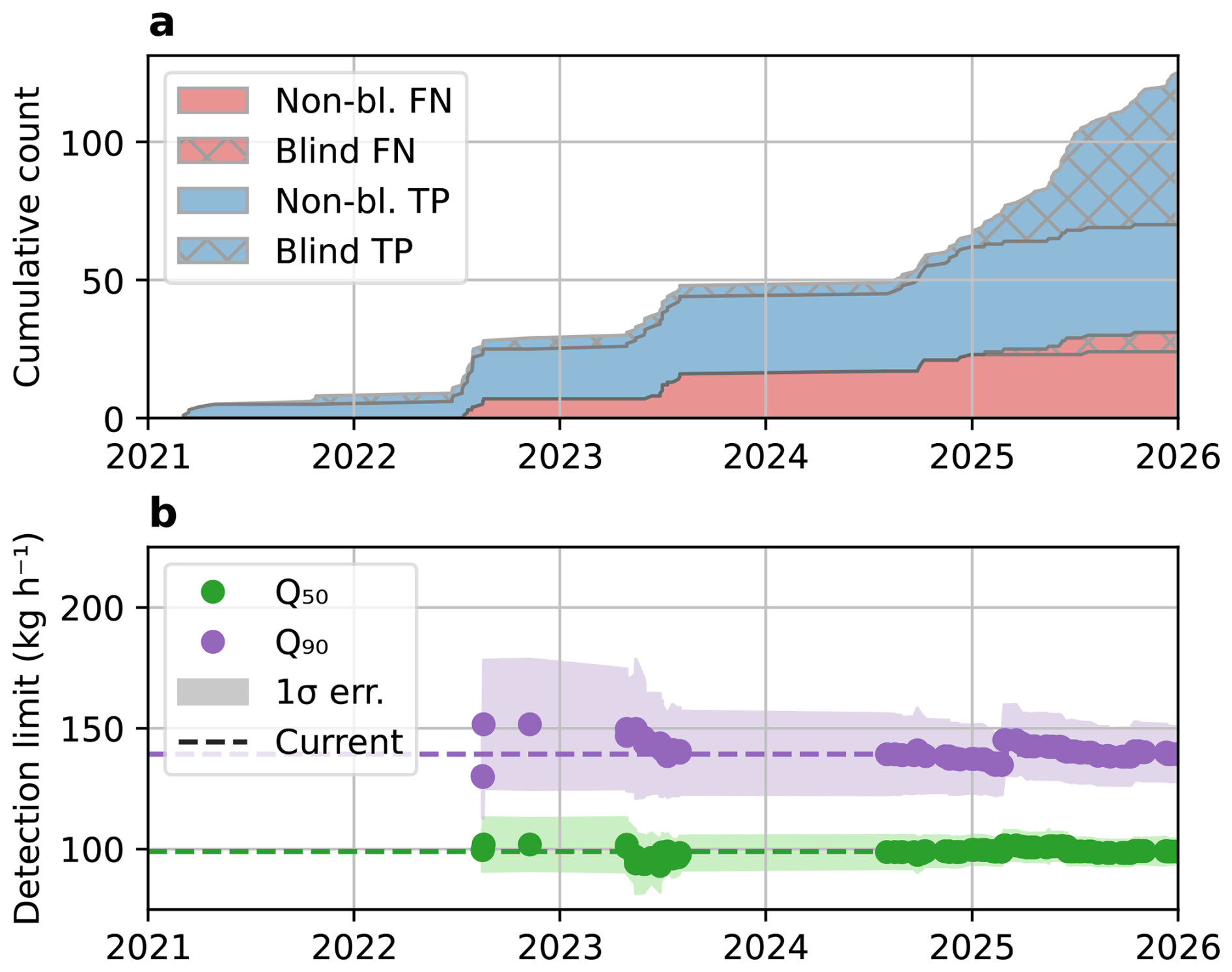
Figure 4 Convergence of the detection limits with the increase of the number of samples between 2021 and 2026. (a) Number of controlled release events accumulated over time, classified as true positive (TP, blue) or false negative (FN, red) and as self-organized (flat) or single-blind (patterned). (b) Detection limits (markers) and associated uncertainties (shaded regions) at PoD = 50 % and 90 %, based on prior controlled release events. Dashed lines represent the current estimate based on all available samples as of May 2026.

Figure 4b shows the corresponding evolution of the detection limit (evaluated at 50 % and 90 % PoD and u = 3 m s⁻¹, using the linear wind offset predictor) based on samples available up to the date on the x-axis. Note that the detection limits are only evaluated starting mid-2022 as the first missed detections (FN) make the analysis possible. After some initial fluctuations, the series converges to the current values Q₅₀= 99.0 ± 5.3 and $Q_{\mathrm{90}}=\mathrm{139.3}\pm \mathrm{11.1}$ kg h⁻¹ as the number of samples increases. The associated uncertainties, shown as shaded regions, also reduce over time, as expected from the increasing sample size. The addition of a large set of single-blind samples in 2025 did not affect the estimated performance metrics significantly, providing stable convergence of Q₅₀ and a modest improvement of Q₉₀. This supports the assumption that the pseudo-blind GHGSat-organized releases, while not truly independent, were treated in a consistent way and are valid inclusions for this analysis.

4 Quantification accuracy

Controlled releases allow us to assess the accuracy of GHGSat's estimated emission rates by comparing them against a precise measurement from a flowmeter on the ground. We base our analysis on the same multi-campaign dataset described in Table 1 and used in the detection limit analysis, restricted to emissions that were successfully detected (true positives) – no rate estimate is performed for undetected plumes. A minor difference from the detection analysis is that the quantification dataset excludes two observations submitted as “detected but not quantified” – one from phase 3 of the Stanford 2025 study and one from the GHGSat/CMC subset – in which the concentration retrieval field was significantly corrupted at the plume location by retrieval artifacts or high cirrus cloud coverage, yet an emission could still be discerned. The quantification analysis is therefore based on a set of 92 true positive samples out of the 94.

The comparison between the metered and estimated source rates is shown in Fig. 5 using three different scales and/or variables: (a, d, g) parity charts in linear scale, (b, e, h) parity charts comparing the logarithm of the metered and estimated rates, and (c, f, i) the log of the estimated/metered error ratio as a function of the metered rate. In all panels, markers indicating individual TP samples are coloured depending on the type of blinding of the experiment (pseudo-blind in blue or single-blind in orange), and ordinary least squares (OLS) regression lines are included for each type as well as for the full dataset (black). A dashed grey line indicates the ideal outcome (estimated equals metered) for visual reference. The first row of subplots (a–c) shows the “reported” rates based on model wind; the second row (d–f) shows the corresponding estimates using wind from a local anemometer; and the third row (g–i) shows the estimates obtained after adjusting the anemometer wind to a 10 m reference height with a logarithmic wind profile. The wind product used is indicated at the top of the legend in each panel. Note that model wind speeds for reported source rates were drawn from GEOS-FP until June 2024, and from OpenWeather for more recent retrievals. Using reported winds, whichever model supplied them, preserves strict blindness of third-party experiments and ensures consistency with published datasets. For multi-phase campaigns in which a source-rate estimate was delivered to the third party both before and after local wind speeds were revealed (Stanford 2021 and 2022), we report the estimates made without local wind information, which are representative of standard commercial processing.

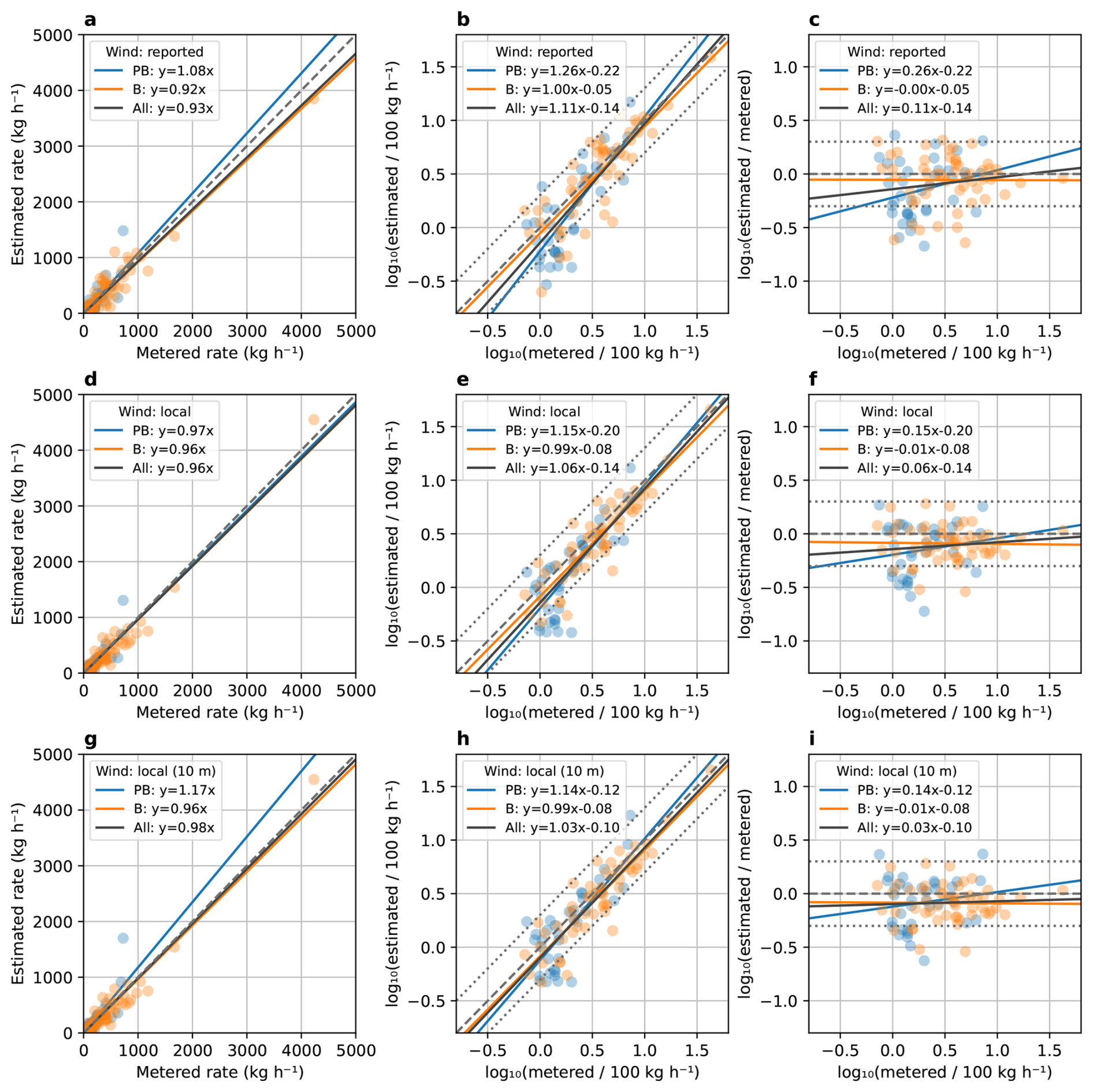
Figure 5 Accuracy of the estimated flow rates (using weather model, local anemometer, and 10 m adjusted anemometer wind speed) compared with ground measurements, represented as (a, d, g) linear scale parity chart, (b, e, h) logarithmic scale parity chart, and (c, f, i) logarithmic error ratio as a function of the logarithm of the metered rate. Rates on the top row (a, b, c) are derived using model wind speed (GEOS-FP or OpenWeather), the middle row (d, e, f) uses local anemometer wind speed, and the bottom row (g, h, i) uses the anemometer wind adjusted to a 10 m reference height with a logarithmic wind profile. The wind product used is also indicated at the top of the legend in each panel. Data samples and ordinary least squares regressions are shown from pseudo-blind tests (PB, blue), single-blind tests (B, orange), and all samples combined (All, black). The dashed grey line represents the parity (1:1) line and the dotted grey lines are the margins for 2× under or overestimation.

Estimated and metered rates agree well overall. With as-reported rates across all true positives, the linear OLS regression has a slope of 0.93 ± 0.03 (standard error on the slope) and a coefficient of determination R²= 0.92. Substituting a local anemometer wind yields a modest improvement in the regression (slope = 0.96 ± 0.02, R²= 0.95) and a reduction in scatter around the parity line. Adjusting the anemometer wind to a 10 m reference height with a logarithmic wind profile (Sect. 3.1.1) brings the slope closer still to unity (slope $=\mathrm{0.98}\pm \mathrm{0.03}$), at a marginally lower R² of 0.93. Those improvements are small relative to the uncertainty of a single source rate estimate (typically on the order of tens of percents) but are in line with the intuitive understanding that more accurate wind measurements result in better emission rate estimates.

One limitation of using a linear scale to assess quantification accuracy is that the linear regression slope is largely determined by the samples with high emission rates. The pseudo-blind subset in Fig. 5g illustrates this: the largest release (metered rate ∼ 725 kg h⁻¹) is an outlier overestimated at 1480 kg h⁻¹, and on its own drives the fitted slope for that subset to 1.17. The logarithmic parity charts (b, e, h) and error-ratio plots (c, f, i) provide clearer visualization at small emission rates. These visualizations reveal a broader scatter and a tendency to underestimate the true rate for the small plumes (relative to the ∼ 100 kg h⁻¹ detection limit), whereas errors for large plumes are more narrowly distributed and more symmetric around the parity line. The following section further investigates this finding and proposes correction strategies to obtain unbiased estimates independently of the emission rate.

4.1 Approaches for emission-rate estimate bias correction

The controlled-release results presented in Fig. 5h–i showed that a subset of emission-rate estimates, concentrated among the smaller sources, were biased low. Because the concentration enhancement from plumes in the ∼ 100 kg h⁻¹ range becomes small relative not only to random noise but also to any systematic bias (e.g., correlated artifacts), a bias in the L2 retrieval is therefore likely to affect small plumes disproportionately. To mitigate this effect while providing evidence to support the L2 bias hypothesis, we implement a local background correction (BGC) that estimates the baseline concentration in the immediate vicinity of each plume by averaging the retrieved concentration over pixels lying more than 3 and fewer than 13 px away from any pixel in the plume mask (implemented using morphological dilations with a square structuring element), forming a 10 px (∼ 300 m) wide annular region around the plume (Fig. 6a). The 3 px buffer region between the plume and background masks avoids the inclusion of diffuse CH₄ enhancements below the masking threshold. A sensitivity analysis of the background region parameters (width and buffer distance) is provided in Sect. S5, showing only minor deviations of the global calibration slope – around ± 2 % over a wide range of widths and buffer distance – supporting the robustness of this approach to specific user configuration.

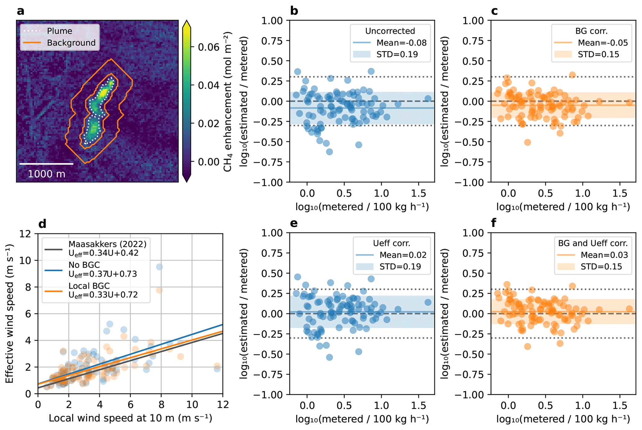
Figure 6 Emission rate bias correction. (a) Illustration of the method for local background correction (BGC) by expanding the plume mask (dotted white line) to generate a padded perimeter (orange line) within which the background concentration is calculated. (b, c, e, f) Logarithmic quantification error ratio for (b) No local BGC, original U_eff; (c) Local BGC, original U_eff; (e) No local BGC, updated U_eff; (f) Local BGC, updated U_eff. (d) Empirical calibration of the effective wind speed against the height-adjusted local wind speed, fitted separately for the uncorrected and background-corrected IME.

The correction is applied to the column density enhancements Ω contained within plume mask M_P, by subtracting the mean column density enhancement within the background mask M_BG:

$$\begin{array}{}\text{(16)}& \mathrm{IME}=A_{\mathrm{pix}}\sum _{i\in M_{\mathrm{P}}}\left({\mathrm{\Omega }}_i-{\stackrel{\mathrm{‾}}{\mathrm{\Omega }}}_{\mathrm{BG}}\right)\end{array}$$

$$\begin{array}{}\text{(17)}& {\stackrel{\mathrm{‾}}{\mathrm{\Omega }}}_{\mathrm{BG}}={\displaystyle \frac{\mathrm{1}}{N_{\mathrm{BG}}}}\sum _{i\in M_{\mathrm{BG}}}{\mathrm{\Omega }}_i,\end{array}$$

where A_pix is the area of a retrieval pixel and N_BG is the number of pixels in the background mask. The effect of this correction on the logarithmic error ratio is shown in Fig. 6b (no BGC applied) and Fig. 6c (local BGC applied). The local background subtraction reduced both the overall scatter (standard deviation of the logarithmic error ratio from 0.19 to 0.15) and the global bias (mean of the logarithmic error ratio from −0.08 to −0.05). Note that in this analysis, source rates were estimated using the height-adjusted local wind speed from anemometers to better highlight the effects of the corrections from the high uncertainty of model wind speed.

The small bias that remains after BGC can always be further compensated by applying a global scaling to the estimated source rates. A natural way to implement this correction when using the IME method is to update the effective wind speed calibration. This calibration was originally tuned from numerical simulation (Maasakkers et al., 2022; Varon et al., 2018), but it can instead be derived empirically from the controlled-release results. For each release we define a “true” effective wind speed as the value of U_eff that would reproduce the metered source rate q from the measured integrated mass enhancement (IME) and plume length:

$$\begin{array}{}\text{(18)}& U_{\mathrm{eff},\mathrm{true}}={\displaystyle \frac{q{L}_{\mathrm{eff}}}{\mathrm{IME}}}.\end{array}$$

We then plot U_eff,true against the height-adjusted local wind speed and fit an ordinary-least-squares linear regression (Fig. 6d). The resulting linear equation U_eff= 0.37 u₁₀+0.73 is obtained when the regression is performed on the IME computed without the local background correction; repeating the fit on the background-corrected IME yields U_eff=  0.33 u₁₀+0.72. Either calibration can then be used as an empirical effective wind speed in the IME method, in place of the numerically calibrated model expressed in Eq. (3); the updated U_eff results shown in Fig. 6e and f use the former and the latter, respectively. Both are equivalently effective at removing the global bias (means of +0.02 and +0.03 respectively), but the standalone version does not address the small rate outliers or reduce the magnitude of the scatter, which stays unchanged from the uncorrected case at 0.19. Combining both corrections – local BGC and U_eff – removes most of the residual global bias: the mean of the logarithmic error ratio rises from −0.08 (Fig. 6b) to +0.03 (Fig. 6f), while the scatter is held at the reduced level of 0.15 (standard deviation of the logarithmic error ratio).

Taken together, the local background correction and the empirically recalibrated effective wind speed constitute a straightforward refinement of the quantification chain that improves accuracy across a wider range of emission rates, recovering the low-rate sources that were previously underestimated without degrading performance at higher rates. Although demonstrated here on GHGSat retrievals, both are transferable with minor adjustments (background segmentation pipeline relative to resolution, wind product) to other point-source imaging systems facing similar biases.

4.2 Comparison of wind sources

Wind speed is a key parameter in source rate estimation and a major contributor to its uncertainty budget (Varon et al., 2018). Many weather forecast and reanalysis models are available as potential wind data sources, but their coverage may be restricted to certain geographic areas, and the latency before data become available can also constrain the choice for a measurement provider with operational delivery requirements. GHGSat currently uses OpenWeather, a third-party aggregator that combines data from multiple weather models, as its primary wind source. While the majority of the releases included in this study were performed in North America, the input models available to the aggregator may vary regionally. To evaluate the robustness of quantification to the choice of wind data, we compare in Fig. 7 the emission-rate estimates from three widely used models: ECMWF reanalysis fifth generation (ERA5, a global reanalysis), ECMWF Integrated Forecasting System (IFS, a global forecast), and NOAA High-Resolution Rapid Refresh (HRRR, a regional forecast covering the continental United States and a portion of Canada that includes the Brooks release site). We also include estimates from a co-located anemometer as a reference. Note that results presented in Fig. 7 do not include the bias correction scheme proposed in the previous section, since the effective wind recalibration would be applied individually for each wind source and result in unbiased estimates for all cases.

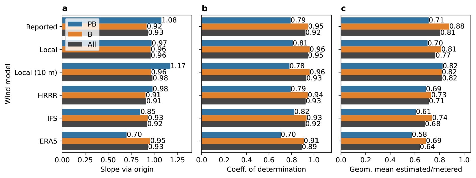
Figure 7 Regression statistics for estimated versus metered source rates under six wind data sources (as-reported, local anemometer, height-adjusted local anemometer, HRRR, IFS, and ERA5): (a) OLS slope through the origin, (b) coefficient of determination R², and (c) geometric mean of the estimated-to-metered ratio. Bar colours distinguish all true positives (black), pseudo-blind (blue), and single-blind (orange) subsets. Values nearer 1 indicate closer agreement with the metered rate.

When aggregated across all true positives, the four model-derived wind sources yield broadly comparable performance: OLS slopes through the origin fall in a narrow 0.91–0.93 range and R² values lie between 0.89 (ERA5) and 0.93 (HRRR), essentially indistinguishable from the as-reported baseline (slope = 0.93, R²=0.92). This insensitivity to the choice of reanalysis or forecast model is a desirable robustness property for operational quantification, since it indicates that emission rate estimates do not depend strongly on the specific wind product available at a given location or latency. As previously discussed, substituting the local anemometer wind raises the slope to 0.96 and R² to 0.95, and adjusting that wind to a 10 m reference height raises the slope further to 0.98, at an R² of 0.93.

The geometric mean of the estimated-to-metered ratio (Fig. 7c) provides a complementary view that is less sensitive to a few high-rate samples than the linear OLS slope. All six wind sources produce geometric means below unity (0.64–0.82 without bias correction across the full dataset). The height-adjusted anemometer wind is the least biased (0.82), ahead of the as-reported baseline (0.81) and the unadjusted anemometer (0.77), while ERA5 shows the largest negative bias (0.64). The magnitude of the bias appears correlated with the spatial resolution of the weather model: 3 km HRRR is least biased, followed by 9 km IFS, while ERA5 (∼ 30 km, 0.25°) shows the largest negative bias. We attribute this trend to spatiotemporal averaging of the wind transport: sub-grid wind speeds resemble a random walk in which instantaneous local speeds exceed the average drift of the centre of mass. This averaging effect being dependent on the grid size, coarser resolution models lead to more underestimation of the local wind.

In summary, this analysis supports that GHGSat's quantification accuracy is robust to the choice among major operationally available wind products – an important property for global deployment, where HRRR-class regional models are not available. A co-located anemometer, if available, measurably improves the regression slope, and more so once its wind is adjusted to a 10 m reference height, but the aggregate gain over global model winds is small. Finally, small differences between models may be driven by their different spatial resolution (grid size). This effect is correctible for any wind model by recalibrating the effective wind speed as described in Sect. 4.1.

5 Conclusions and discussion

This study presents a comprehensive controlled-release assessment of the GHGSat constellation's detection and quantification performance, drawing on a multi-campaign dataset spanning 2021 to 2026 that combines self-organized releases with independent third-party experiments. Framing detection as a probabilistic, conditions-dependent process and grounding the predictor in the Jacob heuristic yields a model that is simple enough to be constrained by the available sample size yet retains physical interpretability across the operational range of the constellation.

The analysis supports several conclusions. First, source rate, wind speed, and retrieval noise are the dominant drivers of detection probability over the operational range examined, while spatial resolution varies too little within nominal viewing conditions to register as an independent predictor once the other three are included. Second, the detection performance is highly consistent across model variants, with Q₅₀ ranging from 89.5 to 102.8 kg h⁻¹ depending on the predictor and link functions. The linear wind offset predictor combined with a log-normal inverse-link had the best fit with the experimental data, in terms of Akaike and Bayesian information criteria. Third, this estimate has converged stably as the sample size has grown, and the addition of a large set of single-blind Stanford samples in 2025 did not significantly shift Q₅₀ or Q₉₀, supporting the validity of pooling self-organized and independently blinded releases.

Because the detection model is explicitly conditions-dependent, the detection limit quoted at controlled-release median conditions should not be read as a single operational figure of merit. The reference conditions used throughout this work (u= 3 m s⁻¹, n= 7.0 mmol m⁻², a= 27.0 m) reflect the distribution of conditions sampled by the controlled-release campaigns, which are on average somewhat more favourable than those encountered across the constellation's global operations. Evaluating the same fitted model over GHGSat's global catalogue and taking the median of the resulting detection limits yields Q₅₀= 159.7 kg h⁻¹, approximately 1.6 times the controlled-release value. The global distribution of conditions is less favourable, with a higher median wind speed (u= 3.2 m s⁻¹) and noise (n= 9.9 mmol m⁻²), while the resolution factor remained similar (a= 27.7 m).

The link function parameters derived here from controlled releases and the associated Q₅₀∼ 100 kg h⁻¹ differs from the survey-mode detection limit reported by the same group of authors (Jervis et al., 2026a), who estimated Q₅₀ ∼460 kg h⁻¹ by fitting a joint model of the emission rate distribution and detection probability to a large ensemble of detected O&G plumes from 2024–2025. The approximately 4.6-fold difference decomposes into the two factors made explicit by the model structure. The first is the difference in observation conditions described above, which accounts for a factor of ∼ 1.6 and is described explicitly by the predictor variables $\mathit{X}=\mathit{\{}q,u,n,a\mathit{\}}$. The second, accounting for the remaining ∼2.9, is the difference in inspection conditions, which are described by link functions parameters $\mathit{\theta }=\left\{\mathit{\mu },\mathit{\sigma }\right\}$. GHGSat distinguishes two modes of data processing. Target-mode applies to commercially contracted observations, where target site locations are known a priori from customers and visually inspected by GHGSat analysts. Survey-mode applies to other regions of the world surveyed by the constellation where both the existence and location of emitting sites may be unknown. They are pre-screened by artificial intelligence (AI), and the detected emissions are validated by human analysts. This mode is relevant for building global measurement-informed inventories based on the full observation capacity of the constellation. Controlled releases provide an estimate most relevant to target-mode detection performance, as they were both processed directly by GHGSat analysts with approximate knowledge of potential release locations. In contrast, the performance estimated by Jervis et al. (2026a) was derived from – and applies to – GHGSat's global catalogue of observations processed in survey-mode.

In summary, the two estimates are not in contradiction but characterize complementary aspects of constellation performance: the controlled-release Q₅₀ reported here quantifies the sensitivity achievable under favourable conditions with known source location, while the survey-mode Q₅₀ of Jervis et al. (2026a) describes the effective detection threshold encountered across the full operational envelope.

On the quantification side, parity analysis across 92 true-positive samples yields an OLS slope of 0.93 and R²= 0.92 with reported model winds, improving to 0.96, R²= 0.95 when a co-located anemometer is substituted, and 0.98, R² = 0.93 with the local wind adjusted to a 10 m reference height. Quantification accuracy is largely insensitive to the choice among the major operationally available wind products (ERA5, IFS, HRRR, and the OpenWeather aggregator) – an important robustness property for global deployment, where regional high-resolution models are not always available. The residual low-rate underestimation is common to all wind sources and correlates with wind-model spatial resolution, pointing to spatiotemporal averaging of sub-grid wind variability as a likely contributor. As a step toward addressing this, we demonstrated a bias correction that combines a local background correction with an empirically recalibrated effective wind speed, reducing both the scatter and the global bias of the quantification and recovering the previously underestimated low-rate sources.

Several limitations qualify the scope of these results and define directions for follow-up work. The controlled releases used here were conducted predominantly at flat, arid, or prairie sites that are representative of many oil and gas production basins but not of typical landfills, coal mines, or urban environments, where topography, land cover, and meteorological conditions differ substantially. Similarly, controlled release experiments included in this study were all point-source in nature, and extension to area sources such as landfills and open-pit mines will require dedicated methodology and validation campaigns (Hossain et al., 2026). These caveats also apply to correction methods, such as effective wind speed recalibration, as wind patterns aggregated into the U_eff function may differ over more complex terrain. However, we note that the same limitation also affects the original numerical calibration (Maasakkers et al., 2022; Varon et al., 2018) that this correction replaces, as it too was derived from WRF-LES simulations that did not include topographic effects. Follow-up investigations are also planned to ensure the annular background correction method applies robustly over the wide variety of scenes encountered in global operations.

Additionally, while the dataset robustly constrains constellation-level detection and quantification models, the per instrument sample size is not sufficient to constrain independent models that would isolate any manufacturing variability between individual payloads. However, we do not consider this a major limitation. Results should indeed be interpreted as representative of the full GHGSat constellation, and this remains a practical and useful outcome since satellites are tasked indistinctively to any targets in nominal operations. Moreover, instrument-to-instrument variability of the PoD is already accounted for to a large extent, through the noise and resolution predictor variables which are inherently instrument- and observation-specific. The fit parameters u₀, μ and σ, which would be derived from hypothetical per-instrument fits, should in contrast be driven mainly by the data analysis pipeline (inspection conditions) and therefore mostly instrument-independent.

In conclusion, these results establish a transparent, statistically grounded baseline for the detection and quantification performance of the GHGSat constellation. The probabilistic, conditions-dependent formulation may be updated as new controlled releases become available and provides a template and methodology for comparing performance across the broader population of methane point-source imagers.