Survival-analysis methods for droplet-freezing data: Kaplan–Meier confidence intervals and non-parametric curve comparison

Droplet-freezing assays underpin immersion-mode ice-nucleation research yet approaches to uncertainty quantification for fraction-frozen curves and derived active-site densities (n_s(T)) are inconsistent. Further, there is currently no rigorous method for significance testing the difference between fraction-frozen curves. To address these issues, we recast droplet-freezing measurements as survival data and apply analysis techniques typically used in medical statistics. Using the Kaplan–Meier estimator, we derive nonparametric pointwise confidence intervals for droplet fraction-frozen without binning or model assumptions. These intervals can also be propagated to cumulative ice-nucleation activity spectra such as  K(T), n_s(T) or n_m(T). Simulations based on fitted literature freezing curves show that Kaplan–Meier intervals have close to nominal coverage over the central portion of fraction-frozen curves, but coverage deteriorates near the ends of the curve where finite experiments contain little information. We also compare several statistical tests for distinguishing between droplet-freezing curves. These tests quantify whether the observed separation between two finite-droplet curves is larger than expected from sampling variability alone. The log-rank test, often used alongside Kaplan–Meier confidence intervals in medical statistics, can be useful for approximately proportional-hazards-like alternatives, but can have low power when curves differ in shape or reflect multiple ice-active populations. We therefore introduce an integrated squared fraction-frozen distance permutation test, which we refer to as the Integrated Squared Difference (ISD) test. This test compares the accumulated squared separation between two empirical fraction-frozen curves directly and does not require proportional hazards. Simulations comparing the ISD test, log-rank and several standard empirical-distribution-function tests show that no single test is most powerful in all situations: performance depends on droplet number, curve shape, and the form of the difference being tested. We recommend reporting fraction-frozen curves with Kaplan–Meier pointwise confidence intervals and droplet numbers, and using the ISD test for general curve comparison. We note finally that a significant global test indicates that two curves differ somewhere over the analysed temperature interval, but does not identify where they differ or why; this still requires inspection of the curves and potentially of normalised spectra.

1 Introduction

Droplet freezing experiments are widely used for the study of immersion mode ice nucleation e.g. (Whale et al., 2015; Bigg, 1953; Vali, 1971; Vali et al., 2015; Polen et al., 2018), a process of critical importance for the glaciation of mixed-phase clouds (Knopf and Alpert, 2023; Herbert et al., 2025). A droplet freezing experiment cools multiple samples of water, usually prepared in a physically identical manner, and measures the temperatures at which they freeze. The unprocessed data produced by these experiments are typically referred to as “fraction-frozen curves” or similar. Experiments of this type have been employed since at least the 1950s (Kuhns, 1966; Bigg, 1953) with droplets ranging in size from picolitres to millilitres (Miller et al., 2021). Many droplet-freezing datasets contain tens to hundreds of droplets per measurement, although the number varies widely with instrument type. Microlitre-scale assays typically freeze on the order of 40–100 droplets per experiment (Whale et al., 2015; Budke and Koop, 2015). High-throughput plate systems can use several hundred wells (Miller et al., 2021; Kunert et al., 2018) and microfluidic systems can generate hundreds to thousands of droplets (Stan et al., 2009; Tarn et al., 2025). On occasion, measurements with fewer than 10 freezing events in larger water volumes are reported e.g. (Kobayashi et al., 2016).

Despite a long period of extensive usage, there is no consensus on how the data produced by droplet freezing assays should be analysed. A particular problem is the calculation of confidence intervals or bands for fraction-frozen curves, and for quantities derived from fraction-frozen curves, such as nucleation rates and deterministic nucleus spectra (Fahy et al., 2022). The purpose of calculating such confidence intervals is to indicate how confident we should be in the value of a calculated datapoint. For instance, a 95 % confidence interval indicates that if we repeated the measurement many times, about 95 % of the intervals we compute would capture the true value.

Fahy et al. (2022) produced a thorough discussion of the various approaches which have been employed to calculate confidence intervals for ice nucleation data. The following briefly summarises this discussion. Where multiple identical experiments have been performed, means and standard deviations of the repeated experiments can be calculated. It is unclear how many experiments would be needed for the central limit theorem to become valid in these cases. Binomial confidence intervals have been calculated by treating fraction-frozen values as binomial ratios and using an adjusted Wald interval (Agresti and Coull, 1998), however most ice nucleation data are not normally distributed, meaning this approach may not always be applicable. Poisson fiducial limits have been used (Koop et al., 1997), which assume that variability in droplet freezing is described by the Poisson distribution. Fahy et al. (2022) state that this approach may not account for all the variables involved in ice nucleation processes. The final approach uses Monte Carlo simulations to simulate experiments based on underlying assumptions about the nature of the ice nucleation process. For instance, Harrison et al. (2016) used ice-active site densities calculated from the original experiments to simulate number distributions. Under the assumption that a droplet freezes when it contains at least one active site, they were able to construct simulated experiments based on the experimental data. An alternative approach suggested by Vali (2019) and applied in various subsequent papers assumes that the number of freezing events in a given temperature interval is Poisson distributed, and generates Poisson distributed random numbers taking the experimentally observed number as the expectation value for the temperature, thereby generating simulated spectra. In both cases, confidence intervals can be calculated by generating hundreds or thousands of simulated experiments and finding quantiles of the simulated data. Fahy et al. (2022) refer to these approaches as `parametric bootstrapping' because they require that ice nucleation measurements be parameterised before Monte Carlo simulations are performed. This necessitates assumptions about the nature of ice nucleation related to distribution of active sites on surfaces and stochasticity or otherwise of the process, or else requires reliance on coarse binning of data in a manner that conflicts with the exponential increase in ice nucleation rate with temperature. To avoid these difficulties Fahy et al. (2022) proposed an “empirical bootstrapping” method for calculating confidence intervals resulting in “studentized” confidence intervals. This method uses the observed list of droplet freezing temperatures with replacement to generate many synthetic experiments, then uses the ensemble to quantify uncertainty (e.g., confidence intervals) without assuming a physical model or a specific error distribution.

Although droplet-freezing datasets can be analysed in several defensible ways, the field lacks a widely adopted statistical framework for reporting uncertainty and quantitatively comparing fraction-frozen curves. Such comparisons are particularly useful for evaluating experimental treatments, such as heat tests (Daily et al., 2022), where the aim is to determine whether treatment produces a statistically detectable change in the freezing behaviour of a sample. Decisions about whether two curves represent meaningfully different freezing behaviour are often based on visual inspection or informal criteria. Visual comparison of fraction-frozen curves remains essential, because it shows where curves differ and suggests possible physical interpretations. However, visual comparison alone can be ambiguous when droplet numbers are small, curves are broad, or confidence intervals overlap over part of the temperature range. It also does not provide a pre-specified false-positive rate or an estimate of statistical power. Formal tests are therefore useful as a complement to graphical interpretation, indicating whether the observed separation between two finite-droplet curves is larger than expected from sampling variability alone.

We recast droplet-freezing measurements as survival data and use this framing in two ways: to calculate Kaplan–Meier pointwise confidence intervals for fraction-frozen and derived cumulative ice-nucleation activity spectra, and to assess non-parametric methods for comparing fraction-frozen curves. In doing so, we suggest the well-established log-rank test as a useful comparison tool in some contexts and introduce an integrated squared fraction-frozen distance permutation test, which we refer to as the Integrated Squared Difference (ISD) test, for cases where a more general curve-based comparison is required. To assess these methods, we use synthetic droplet-freezing experiments generated from fitted representations of literature freezing curves. This allows us to test Kaplan–Meier interval coverage, false-positive rates, and false-negative rates for realistic curve shapes while retaining known underlying generating distributions.

2 Statistical Background

2.1 The Kaplan–Meier estimator applied to droplet freezing data

In a typical set of droplet freezing experiments, multiple aliquots of water are exposed to a systematically decreasing temperature, allowing observation (typically visual) of the onset and distribution of freezing events across the sample set. The fraction-frozen is calculated as:

$$\begin{array}{}\text{(1)}& f\left(T\right)={\displaystyle \frac{N_{\mathrm{F}}\left(T\right)}{N_{\mathrm{0}}}}\end{array}$$

where N_F(T) is the number of droplets frozen at temperature T and N₀ is the total number of droplets, frozen or unfrozen, present in the experiment (Vali et al., 2015). A typical dataset where a survival curve might be employed would have n(t_j) subjects at risk of failure at time t_j and d(t_j) failures at time t_j (Kalbfleisch and Prentice, 2002). The nonparametric likelihood estimate of the survivor function, the probability that a sample survives longer than time t, is then

$$\begin{array}{}\text{(2)}& \widehat{S}\left(t\right)={\prod }_{t_j\le t}\left({\displaystyle \frac{n\left(t_j\right)-d\left(t_j\right)}{n\left(t_j\right)}}\right).\end{array}$$

The derivation of this equation may be found in Kalbfleisch and Prentice (2002) and also the original paper on the Kaplan–Meier estimator (Kaplan and Meier, 1958). For continuously and steadily cooled droplet freezing experiments T is directly proportional to t. As such, the survivor function for droplet freezing data as a function of temperature is

$$\begin{array}{}\text{(3)}& \widehat{S}\left(T\right)={\prod }_{T_j\ge T}\left({\displaystyle \frac{N_{\mathrm{U}}\left(T_j\right)-N_{\mathrm{F}}\left(T_j\right)}{N_{\mathrm{U}}\left(T_j\right)}}\right).\end{array}$$

where N_U(T) is the number of unfrozen droplets at temperature T and N_F(T) is the number of droplets that freeze at temperature T. Note that f(T) is equal to $\mathrm{1}-\widehat{S}\left(T\right)$. Equation (3) has the advantage that it is valid for “censored” data, so can be used for datasets where it is not known whether droplets freeze or not. In principle, droplets can also be added part-way through an experiment. Censoring could arise if an experiment ended before all droplets had frozen, for example because the instrument reached its minimum temperature, although good experimental design should normally avoid such situations.

2.2 Confidence intervals of the Kaplan–Meier Estimator

As discussed above, confidence intervals are useful for visualising the likely values which fraction-frozen may take. Standard approaches for the calculation of the variance of $\widehat{S}\left(t\right)$ may yield values outside the possible range of 0 to 1. As such the confidence intervals for the Kaplan–Meier estimator are usually calculated by applying the asymptotic normal distribution to a transformation of $\widehat{S}\left(t\right)$ for which the range is unrestricted. The same approach may be adopted for calculation of confidence intervals for $\widehat{S}\left(T\right)$ and therefore f(T). Assuming that the probability of freezing is reasonably approximated by $N_{\mathrm{F}}/N_{\mathrm{U}}$ and the probability of freezing at each timestep is independent, the asymptotic variance of $\text{ln}[-\text{ln}\widehat{S}(T\left)\right]$ may be calculated as

$$\begin{array}{}\text{(4)}& {\widehat{\mathit{\sigma }}}^{\mathrm{2}}\left(T\right)={\displaystyle \frac{{\sum }_{T_j}\frac{N_{\mathrm{F}}\left(T_j\right)}{N_{\mathrm{U}}\left(T_j\right)\left(N_{\mathrm{U}}\right(T_j)-N_{\mathrm{F}}(T_j\left)\right)}}{{\left\{{\sum }_{T_j}\text{ln}\left(\frac{N_{\mathrm{U}}\left(T_j\right)-N_{\mathrm{F}}\left(T_j\right)}{N_{\mathrm{U}}\left(T_j\right)}\right)\right\}}^{\mathrm{2}}}}\end{array}$$

where the sums are calculated between T and the first value of T at which a freezing event occurs (Kalbfleisch and Prentice, 2002). In cases where there is no censorship, as there won't be for most ice nucleation measurements, Eq. (4) reduces to

$$\begin{array}{}\text{(5)}& {\widehat{\mathit{\sigma }}}^{\mathrm{2}}\left(T\right)={\displaystyle \frac{\mathrm{1}-\widehat{S}\left(T\right)}{N_{\mathrm{0}}\widehat{S}\left(T\right)\left(\text{ln}\widehat{S}\right(T){)}^{\mathrm{2}}}}.\end{array}$$

The confidence intervals for $\widehat{S}\left(T\right)$ are then given by $\left[\widehat{S}\right(T{)}^{\text{exp}(+z_{\mathit{\alpha }/\mathrm{2}}\widehat{\mathit{\sigma }}(T\left)\right)}$, $\widehat{S}\left(T{)}^{\text{exp}(-z_{\mathit{\alpha }/\mathrm{2}}\widehat{\mathit{\sigma }}(T\left)\right)}\right]$ where $z_{\mathit{\alpha }/\mathrm{2}}$ is the inverse of the standard normal cumulative distribution, which takes values of 1.96 for a 95 % confidence interval and 1.64 for a 90 % confidence interval. The confidence interval for f(T) may be found as $[\mathrm{1}-\widehat{S}(T{)}^{\text{exp}(+z_{\mathit{\alpha }/\mathrm{2}}\widehat{\mathit{\sigma }}(T\left)\right)},\mathrm{1}-\widehat{S}\left(T{)}^{\text{exp}(-z_{\mathit{\alpha }/\mathrm{2}}\widehat{\mathit{\sigma }}(T\left)\right)}\right]$. A difficulty with this approach is that no confidence interval can be calculated when f(T)=1 because the logarithm is undefined at $\widehat{S}\left(T\right)=\mathrm{0}$. For plotting purposes, we assign the final point the same interval as the penultimate point. This is a pragmatic plotting convention rather than a formally derived confidence interval at f(T)=1. It affects only the final plotted point and does not alter the curve-comparison tests or any conclusions, because these tests are calculated from the observed freezing temperatures and empirical fraction-frozen curves rather than from the confidence intervals. The final point should therefore not be interpreted as having a formally calibrated confidence interval. We calculated confidence intervals for f(T) in the manner described here in Kinney et al. (2024). We note that the shaded regions shown in the figures later in this paper connect the calculated pointwise confidence intervals for visual clarity and should not be interpreted as simultaneous confidence bands over the full temperature range (Sachs et al., 2022).

Droplet fraction-frozen data are often used to calculate surface density of sites active above temperature T, n_s(T) to allow comparison of measurements conducted on different instruments or in different concentration regimes. This can be calculated as

$$\begin{array}{}\text{(6)}& n_{\mathrm{s}}\left(T\right)={\displaystyle \frac{-\text{ln}(\mathrm{1}-f(T\left)\right)}{A}}\end{array}$$

Where A is the total surface area of INPs in a sample unit, usually given in cm² (Vali et al., 2015). Other quantities, for instance mass, can be used to normalise instead of A. The equivalent normalised to the droplet volume is usually referred to as K(T), the cumulative nucleus spectrum, while equivalent normalised to mass per sample unit is referred to as n_m(T). To calculate the confidence interval for n_s(T) or other monotonic equivalents equation 6 may be applied, replacing f(T) with its confidence interval. It is worth noting that the abovementioned difficulty with the confidence interval of the final freezing droplet is avoided as n_s(T) and equivalents also cannot be calculated when f(T)=1. Kaplan–Meier confidence intervals propagate naturally to cumulative spectra because these are direct transformations of f(T). Differential spectra are less straightforward because they require an additional differencing, binning, smoothing, or fitting step, and their interpretation depends on how the freezing-temperature data are represented, as discussed by Vali (2023) in relation to Fahy et al. (2022). For this reason, we focus here on fraction-frozen curves and cumulative spectra, where the transformation from the Kaplan–Meier estimator is direct.

The approach to calculating confidence intervals is non-parametric in nature, meaning no assumption is made about the distribution of freezing temperatures. It shares this feature with the bootstrapping approach of Fahy et al. (2022) but is simpler to implement and understand, requiring no generation of synthetic experiments or other choices regarding data handling.

2.3 The log-rank test

A common question in the analysis of ice nucleation data is “are these two fraction-frozen curves different?”. For instance, an investigator may wish to establish whether a chemical treatment changes the nucleation temperature of a specific ice nucleator significantly or determine whether a measurement conducted in the presence of an ice nucleator is distinct from the background ice nucleation induced by the instrument. To date, such comparison has typically been conducted visually or by use of ad-hoc statistical comparison of curves. Here, we apply a standard approach for comparing survival curves (Kalbfleisch and Prentice, 2002) to the comparison of fraction-frozen curves, potentially constituting a more rigorous method for establishing whether the population of ice nucleators generating fraction-frozen curves are different in nature. As with the Kaplan–Meier estimator, the log-rank test breaks down the experiment into distinct events and looks at the set of droplets at risk immediately before a given event occurs. In the case of the Kaplan–Meier method, this set is used to calculate the conditional probability of a droplet surviving beyond temperature T. In contrast, the log-rank test estimates the expected number of events at temperature T under the null hypothesis that two freezing curves are identical. It then compares the expected number of freezing events with the observed number to assess whether curves differ significantly.

Suppose that we want to test the null hypothesis that droplet freezing experiments represented by survivor functions ${\widehat{S}}_{\mathrm{0}}\left(T\right)$ and ${\widehat{S}}_{\mathrm{1}}\left(T\right)$ have identical underlying freezing probabilities. At each freezing temperature we first compute how many unfrozen droplets there are at that temperature as

$$\begin{array}{}\text{(7)}& N_{\mathrm{U},\text{tot}}\left(T\right)=N_{\mathrm{U},\mathrm{0}}\left(T\right)+N_{\mathrm{U},\mathrm{1}}\left(T\right).\end{array}$$

We then compute the total number of freezing events as

$$\begin{array}{}\text{(8)}& N_{\mathrm{F},\text{tot}}\left(T\right)=N_{\mathrm{F},\mathrm{0}}\left(T\right)+N_{\mathrm{F},\mathrm{1}}\left(T\right).\end{array}$$

Under the null hypothesis, the expected number of freezing events in experiment 1 at temperature T is

$$\begin{array}{}\text{(9)}& E_{\mathrm{1}}\left(T\right)=N_{\mathrm{U},\mathrm{1}}\left(T\right){\displaystyle \frac{N_{\mathrm{F},\text{tot}}\left(T\right)}{N_{U{,}_{\text{tot}}}\left(T\right)}}\end{array}$$

and the variance of the expected number of events at temperature T is

$$\begin{array}{}\text{(10)}& V_i\left(T\right)={\displaystyle \frac{N_{\mathrm{U},\mathrm{0}}\left(T\right)N_{\mathrm{U},\mathrm{1}}\left(T\right)N_{\mathrm{F},\text{tot}}\left(N_{\mathrm{U},\text{tot}}\right(T)-N_{\mathrm{F},\text{tot}}(T\left)\right)}{N_{\mathrm{U},\text{tot}}\left(T{)}^{\mathrm{2}}\right(N_{\mathrm{U},\text{tot}}\left(T\right)-\mathrm{1})}}.\end{array}$$

The log-rank score is the signed sum of observed-minus-expected events across all event temperatures. The test statistic is the square of this total score divided by the sum of the variance contributions (Kalbfleisch and Prentice, 2002).

$$\begin{array}{}\text{(11)}& {\mathit{\chi }}^{\mathrm{2}}={\displaystyle \frac{(\sum N_{\mathrm{F},\mathrm{1}}-E_{\mathrm{1}}{)}^{\mathrm{2}}}{\sum V_i}}\end{array}$$

The χ² statistic with one degree of freedom is used to calculate the p-value (Kalbfleisch and Prentice, 2002). This may be done using statistical tables or (for example) the scipy function scipy.stats.chi2.sf. The resulting p-value quantifies the probability of observing differences between two freezing curves at least as large as those measured, assuming the null hypothesis. The use of the χ² distribution relies on the asymptotic result that the sum of differences in the numerator in the test statistic is normally distributed. Hence, a sufficiently large number of droplets are required in the experiment to assume this consequence of the central limit theorem applies.

2.4 Limitations of the log-rank test

The ordinary log-rank test is a standard non-parametric test for comparing two survival curves. It is commonly used because it is simple, well understood, and does not require a parametric model for the event-time distribution. However, it is not a general-purpose test for all possible differences between two curves. The log-rank test is most powerful when the two groups have approximately proportional hazards, meaning that the ratio of the conditional event rates is roughly constant over the analysis variable (Kalbfleisch and Prentice, 2002). In the present context, this would mean that the ratio of conditional freezing probabilities for two droplet-freezing experiments is approximately constant across the temperature range.

This assumption is unlikely to be true for ice-nucleation data. Many droplet-freezing curves are likely to reflect more than one ice-nucleation active population. In addition, background freezing may dominate one part of the temperature range, while the nucleating material of interest dominates another. A treatment may also change the high-temperature part of a freezing curve without changing the low-temperature part, or vice versa. In such situations, the relative conditional freezing probability of two samples can vary strongly with temperature. The proportional-hazards assumption will, therefore, almost certainly fail even when the two plotted fraction-frozen curves do not obviously cross. Crossing curves are only a clear visual example of a broader difficulty.

The practical consequence is that the ordinary log-rank test has reduced power in most applications to fraction-frozen data. This issue is well known in the survival-analysis literature, particularly for crossing survival curves and for cases where differences are concentrated in only part of the event distribution (Dormuth et al., 2022). The reason is that the ordinary log-rank statistic is based on a signed sum of observed-minus-expected event counts. If one sample has more freezing events than expected at relatively high temperatures but fewer than expected at lower temperatures, these positive and negative contributions can partly cancel. In such cases, a non-significant log-rank result should not be interpreted as strong evidence that two fraction-frozen curves are the same.

It is also important to be clear about the question being asked. The log-rank test gives a global and non-directional test of whether two droplet-level datasets are consistent with the same underlying freezing-temperature distribution. It does not say where the curves differ, which sample is more active over a particular temperature interval, or what physical mechanism is responsible. These questions require inspection of the curves themselves and, where appropriate, comparison of derived quantities such as K(T), n_s(T) or n_m(T). Pointwise confidence intervals and confidence bands are also useful for visual interpretation, although visual overlap or non-overlap of intervals is not the same as a pre-specified global hypothesis test (Sachs et al., 2022; Cumming, 2009).

We therefore treat the ordinary log-rank test as one useful comparison, rather than as a universal method for comparing droplet-freezing datasets. It is a poor choice when the curves cross, nearly cross, or when there is clear evidence that different ice-active populations dominate in different parts of the temperature range.

2.5 Alternative tests considered

Because the ordinary log-rank test is not expected to perform equally well for all possible differences between freezing curves, we compared it with several other two-sample tests. Mathematical details of the tests are given in the SI. We chose tests that are well established and easy to implement in Python, because a useful method for droplet-freezing analysis should be straightforward to apply. The tests considered here are non-parametric, but they emphasise different aspects of the data.

The Kolmogorov–Smirnov test compares the maximum vertical separation between two empirical distribution functions (Conover, 1999). Since the fraction-frozen curve is directly related to the empirical distribution of freezing temperatures, the Kolmogorov–Smirnov statistic can also be interpreted as the largest pointwise separation between two empirical fraction-frozen curves. This makes it sensitive to localised differences. However, because it uses only the maximum separation, it may be less sensitive to smaller differences that are spread over a wide temperature interval (Conover, 1999).

The Cramér–von Mises test measures an integrated squared difference between empirical distribution functions (Anderson, 1962). It therefore accumulates differences across the full freezing-temperature distribution rather than focusing only on the single largest separation like the Kolmogorov–Smirnov test (Anderson, 1962). This makes it a useful comparator for cases where two fraction-frozen curves are moderately separated over a broad temperature range. The Anderson–Darling k-sample test is related to the Cramér–von Mises test, but gives relatively greater weight to differences in the tails of the pooled distribution (Scholz and Stephens, 1987).

We also considered a Fleming–Harrington weighted log-rank test (Fleming and Harrington, 2013). Weighted log-rank tests generalise the ordinary log-rank test by applying a weight to each observed-minus-expected contribution. For Fleming–Harrington weights,

$$\begin{array}{}\text{(12)}& w_j={\widehat{S}}_{\text{pool}}{\left(t_j^{-}\right)}^p{\left[\mathrm{1}-{\widehat{S}}_{\text{pool}}\left(t_j^{-}\right)\right]}^q,\end{array}$$

where ${\widehat{S}}_{\text{pool}}\left(t_j^{-}\right)$ is the pooled Kaplan–Meier survival estimate immediately before event time t_j. In this work we focus on FH(1,0), which places greater weight on early events in survival time. Since we analyse freezing temperatures using the survival-style transformation $t=-T$, early event times correspond to higher-temperature freezing events.

In principle, weighted log-rank tests are attractive because they allow one part of the freezing spectrum to be emphasised. For example, one might choose a weighting that gives greater importance to higher-temperature freezing events if there were a clear prior reason to expect a difference specifically in the warmest part of the spectrum. However, this is also the main difficulty with applying weighted log-rank tests to droplet-freezing data. In most cases we do not have a sufficiently specific theory to say in advance what the weighting should be. Choosing a weighting after inspecting the curves would make the resulting test difficult to interpret, because the hypothesis being tested would no longer be clearly pre-specified. For this reason, we include FH(1,0) in the simulations as a useful comparator and as an illustration of how changing the log-rank weighting can affect power but do not suggest weighted log-rank tests as a general solution for comparing droplet-freezing curves. Where there is no clear prior reason to emphasise a particular temperature region, a direct curve-distance test or a standard empirical-distribution test is easier to interpret.

2.6 The Integrated Squared Difference (ISD) test

In the case of non-proportional hazards and most significantly when curves cross, the ordinary log-rank test can have low power because the test statistic includes sums over oppositely-signed observed-minus-expected contributions. The Kolmogorov–Smirnov test, by contrast, uses only the largest pointwise separation and so does not fully use the fact that the curves may be separated over a broad interval. The Cramér–von Mises and Anderson–Darling tests are closer to what we want, because they accumulate differences across the empirical distributions. However, they do this on the empirical-distribution, or rank, scale rather than directly over temperature. Anderson–Darling also gives additional weight to the tails, which may or may not be where the physically important difference lies. For droplet-freezing data, where the fraction-frozen curve as a function of temperature is usually the object being interpreted, it is useful to have a test that measures the accumulated separation between those curves directly.

We therefore introduce a simple additional test based directly on the distance between two fraction-frozen curves. The test statistic measures the integrated squared separation between the two fraction-frozen curves over the temperature range being compared. As such, differences at different temperatures all contribute positively to the test statistic. This is conceptually similar to the Cramér–von Mises construction, though it operates on the fraction-frozen curve as a function of temperature, rather than on ranked data. Consequently, the test statistic has units of temperature. In contrast to the previously mentioned tests, which were developed under the constraint that analytical, asymptotic null distributions could be derived, it uses permutation statistics to estimate the null distribution numerically and compute a p-value for the global null hypothesis that the two droplet-freezing datasets are exchangeable samples from the same underlying freezing-temperature distribution. This facilitates the use of this simple and intuitive test statistic, specifically developed to avoid the dependence of the log-rank test on the assumption of proportional hazards. The aim is not to replace all other tests, but to provide a comparison that is closely matched to the way droplet-freezing data are usually displayed and interpreted.

Consider two droplet-freezing experiments indexed by

$$\begin{array}{}\text{(13)}& g\in \mathit{\{}\mathrm{0},\mathrm{1}\mathit{\}},\end{array}$$

with n_g droplets and observed freezing temperatures

$$\begin{array}{}\text{(14)}& X_{g\mathrm{1}},X_{g\mathrm{2}},\mathrm{\dots },X_{g{n}_g}.\end{array}$$

For a temperature T, define the empirical fraction-frozen curve as

$$\begin{array}{}\text{(15)}& {\widehat{f}}_g\left(T\right)={\displaystyle \frac{N_g\left(T\right)}{n_g}}.\end{array}$$

Equivalently, N_g(T) is the number of observed freezing temperatures in experiment g satisfying X_gk≥T. If one instead plots the survivor function (or fraction unfrozen), ${\widehat{S}}_g\left(T\right)=\mathrm{1}-{\widehat{f}}_g\left(T\right)$, the squared difference statistic defined below is unchanged because

$$\begin{array}{}\text{(16)}& {\widehat{f}}_{\mathrm{0}}\left(T\right)-{\widehat{f}}_{\mathrm{1}}\left(T\right)=-\left[{\widehat{S}}_{\mathrm{0}}\left(T\right)-{\widehat{S}}_{\mathrm{1}}\left(T\right)\right].\end{array}$$

Let $\mathcal{T}=[T_{\text{min}},T_{\text{max}}]$ denote the common temperature interval over which the two curves are compared. We define the ISD statistic as

$$\begin{array}{}\text{(17)}& Q_{\mathrm{f}}=\underset{\mathcal{T}}{\int }{\left[{\widehat{f}}_{\mathrm{0}}\left(T\right)-{\widehat{f}}_{\mathrm{1}}\left(T\right)\right]}^{\mathrm{2}}\mathrm{d}T.\end{array}$$

Large values of Q_f indicate that the two fraction-frozen curves are separated over a substantial part of the temperature interval.

In practice, Eq. (17) is evaluated numerically on a regular temperature grid,

$$\begin{array}{}\text{(18)}& T_{\mathrm{1}},T_{\mathrm{2}},\mathrm{\dots },T_M,\end{array}$$

with grid spacing ΔT. In the Jupyter notebook implementing the test we use

$$\begin{array}{}\text{(19)}& Q_{\mathrm{f}}\approx {\sum }_{m=\mathrm{1}}^{M-\mathrm{1}}{\left[{\widehat{f}}_{\mathrm{0}}\left(T_m\right)-{\widehat{f}}_{\mathrm{1}}\left(T_m\right)\right]}^{\mathrm{2}}\mathrm{\Delta }T.\end{array}$$

The same grid and temperature interval are used for the observed data and for all permutations. The absolute value of Q_f depends on the selected temperature interval because the statistic has units of temperature. The interval defines the portion of the curves being compared and should therefore be specified before testing and applied identically to the observed data and all permutations.

The temperature grid is used only for numerical evaluation of the integral and does not divide the data into independently tested bins. Consequently, reducing ΔT does not inherently increase the likelihood of obtaining a significant result: as the grid is refined, the larger number of evaluation points is offset by the factor ΔT, and the sum converges towards the integral in Eq. (17). The same temperature interval and grid are also used for the observed statistic and for every permutation. Conversely, an excessively coarse grid could fail to resolve differences between the curves. The implementation supplied with this work uses ΔT = 0.01 °C, which is small relative to the temperature scale over which typical droplet-freezing curves vary. For alternative implementations, we recommend choosing sufficiently small ΔT relative to the narrowest curve feature of interest. Numerical convergence can readily be checked by repeating the calculation using a finer grid.

The null hypothesis is

$$\begin{array}{}\text{(20)}& H_{\mathrm{0}}:f_{\mathrm{0}}\left(T\right)=f_{\mathrm{1}}\left(T\right)\text{ for\hspace{0.17em}\hspace{0.17em}all }T\in \mathcal{T},\end{array}$$

or equivalently that the two droplet sets are exchangeable samples from the same freezing-temperature distribution over the analysed interval. To obtain a p value, the observed freezing temperatures are pooled,

$$\begin{array}{}\text{(21)}& \mathcal{X}=\mathit{\{}{X}_{\mathrm{01}},\mathrm{\dots },X_{\mathrm{0}{n}_{\mathrm{0}}},X_{\mathrm{11}},\mathrm{\dots },X_{\mathrm{1}{n}_{\mathrm{1}}}\mathit{\}},\end{array}$$

then randomly relabelled into two groups of sizes n₀ and n₁. For each permutation $b=\mathrm{1},\mathrm{\dots },B$, the empirical curves and integrated squared distance $Q_{\mathrm{f}}^{\left(b\right)}$ are recalculated. The Monte-Carlo permutation p value is then

$$\begin{array}{}\text{(22)}& p_{\text{perm}}={\displaystyle \frac{\mathrm{1}+{\sum }_{b=\mathrm{1}}^B\mathrm{1}\left\{Q_{\mathrm{f}}^{\left(b\right)}\ge Q_{\mathrm{f}}^{\text{obs}}\right\}}{B+\mathrm{1}}}.\end{array}$$

The addition of 1 to the numerator and denominator prevents a p-value of exactly zero when a finite number of random permutations is used (Phipson and Smyth, 2010). Note that the estimation of the null distribution via permutation statistics means that the test should be used with caution at very low droplet number. At very low droplet numbers, the number of distinct label permutations is small, resulting in a discrete null distribution and coarse attainable p-values. Power is also necessarily limited because the empirical curves contain little information. For equal group sizes, rejection at α=0.05 is impossible when n≤3 droplets per curve and is possible but highly discrete at n=4. Results obtained with five or fewer droplets per curve should therefore be interpreted very cautiously.

The ISD test is a global test, meaning a significant result indicates that the two fraction-frozen curves differ somewhere over the analysed temperature interval. It does not, by itself, identify the temperature region responsible for the difference or explain the physical origin of the difference. Those questions still require inspection of the curves and, where appropriate, comparison of K(T), n_s(T), or n_m(T) or other physically normalised quantities. The main reason for including this test is therefore pragmatic. It tests the quantity that is most commonly plotted, its power does not depend on the assumption of proportional hazards, and it avoids the cancellation problem that can affect the ordinary log-rank test. We use it here as a general-purpose global comparison of two directly comparable droplet-freezing experiments when no more specific directional or temperature-localised alternative is assumed.

3 Results and discussion

3.1 Simulation strategy

To assess the Kaplan–Meier confidence intervals and the curve-comparison tests in a controlled way, we used synthetic droplet-freezing experiments generated from smooth fitted representations of real droplet-freezing datasets. This approach has the advantage that the underlying freezing-temperature distribution is known, while the simulated experiments still resemble datasets encountered in practice.

We fitted dual-Gaussian mixture functions to three published microlitre-scale droplet-freezing datasets: a background freezing curve (Whale, 2024), Betula pendula pollen washing water (Kinney et al., 2024) and BCS375 feldspar (Harrison et al., 2016) These datasets were chosen because they cover a useful range of fraction-frozen curve shapes. The Betula pendula pollen washing water curve is very steep, the background curve is broader, and the BCS375 feldspar curve is spread over a still wider temperature interval. The fitted functions and parameters are shown in Fig. S1 in the Supplement. The dual-Gaussian functions are not intended as mechanistic models of ice nucleation but are flexible empirical descriptions of realistic freezing curves from which repeated synthetic experiments can be generated.

We used these fitted distributions in two ways. First, we assessed the Kaplan–Meier pointwise confidence intervals by repeatedly sampling synthetic droplet-freezing experiments from each fitted distribution. For each simulated experiment, we calculated Kaplan–Meier confidence intervals for f(T). We also propagated these intervals to the volume-normalised cumulative nucleus spectrum, K(T), by applying the standard transformation to the upper and lower confidence limits of f(T). Because the fitted generating distribution is known, the simulated intervals can be compared directly with the underlying curve. This allows us to estimate empirical coverage: the fraction of repeated experiments in which the nominal 95 % interval contains the underlying value.

Second, we used the same fitted distributions to compare statistical tests for differences between two fraction-frozen curves. Under null scenarios, both synthetic experiments were sampled from the same fitted distribution, allowing us to estimate false-positive rates. Under alternative scenarios, the two experiments were sampled from different distributions, or from shifted or mixture-modified versions of the fitted distributions, allowing us to estimate power and false-negative rates. In all cases, the aim was not to reproduce every possible droplet-freezing dataset, but to test the methods against curve shapes and sample sizes that are realistic for ice-nucleation experiments.

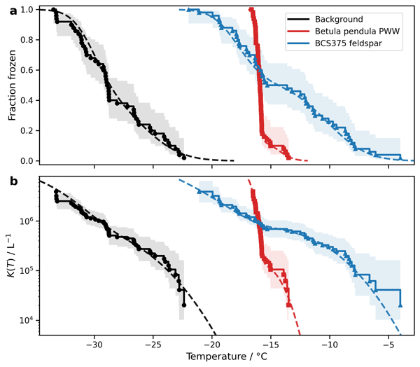
Figure 1 Example 50-droplet synthetic droplet-freezing experiments generated from known underlying freezing curves resembling a microlitre droplet freezing assay instrument background, Betula pendula pollen washing water, and BCS375 feldspar. (a) Fraction-frozen, f(T) with 95 % pointwise Kaplan–Meier confidence intervals. (b) Corresponding cumulative ice-nucleation activity, K(T), obtained by transforming f(T). Solid symbols and step curves show example simulated experiments; dashed curves show the known underlying functions. Shaded regions connect the 95 % pointwise Kaplan–Meier confidence intervals for visual clarity and should not be interpreted as simultaneous confidence bands.

3.2 Empirical coverage assessment of Kaplan–Meier confidence intervals

Figure 1 shows example synthetic experiments generated from the fitted freezing-temperature distributions described above.

The solid symbols and step curves show one 50-droplet simulated droplet-freezing experiment for each underlying distribution, while the dashed curves show the known underlying functions from which the simulated freezing temperatures were generated. The shaded regions show the corresponding 95 % pointwise Kaplan–Meier confidence intervals. In Fig. 1a, the intervals are shown for fraction-frozen. In Fig. 1b, the same intervals have been transformed to K(T). The examples illustrate two useful features of the method. First, the intervals behave sensibly for curves of very different steepness and temperature range. Second, the transformation to K(T) naturally magnifies uncertainty in regions where f(T) approaches 0 or 1, reflecting the well-known sensitivity of logarithmic ice-nucleation spectra to the ends of fraction-frozen curves. Figure S2 in the Supplement shows pointwise Kaplan–Meier confidence intervals for 5 and 100 droplets for the three experiments, to illustrate how the confidence intervals vary with both slope of the fraction-frozen curve and droplet number.

Figure 2 Average empirical pointwise coverage of nominal 95 % Kaplan–Meier confidence intervals as a function of droplet number for synthetic droplet-freezing experiments based on the three underlying curves shown in Fig. 1. Coverage was calculated from repeated synthetic experiments as the fraction of intervals containing the known underlying value.

To quantify the interval performance, we generated repeated synthetic experiments for each underlying curve and droplet number. At each temperature grid point, we calculated the fraction of repeated experiments for which the nominal 95 % Kaplan–Meier interval contained the known underlying value. This fraction is the empirical pointwise coverage. Figure 2 shows the average empirical coverage as a function of droplet number for the three underlying freezing curves. For very small droplet numbers, the average coverage is below the nominal 0.95 level and the curves are necessarily coarse because each individual freezing event represents a large fraction of the experiment. However, the empirical coverage approaches the nominal level as droplet number increases. For these examples, coverage is already close to 0.95 for typical droplet numbers used in many droplet-freezing experiments, and continues to improve gradually as the number of droplets increases.

Figure 3 Temperature-dependent empirical coverage for the background-freezing example with 50 droplets. (a) Coverage of nominal 95 % pointwise Kaplan–Meier confidence intervals for f(T), compared with the known underlying fraction-frozen curve. (b) Coverage after transformation to K(T), compared with the known underlying K(T). Coverage is close to nominal over the central part of the fraction-frozen curve but deteriorates near the extremes, where finite experiments provide little information and where the transformation to K(T) is especially sensitive.

We find also that the coverage is not uniform across the entire temperature range. Figure 3 shows the coverage as a function of temperature for the background-freezing example. For f(T), the intervals have close to nominal coverage over most of the central part of the curve. Coverage deteriorates near the ends of the curve, where the true fraction-frozen is close to either 0 or 1 and where finite experiments contain little information about the exact tail behaviour. This is expected for pointwise intervals on an empirical survival curve. The same issue is more pronounced after transformation to K(T), because the logarithmic transformation is particularly sensitive to values of f(T), close to 0 or 1. In addition, K(T), is undefined at f(T)=0, and singular as f(T) approaches 1. These edge effects are therefore not specific to the Kaplan–Meier estimator, but reflect the limited information content of finite droplet-freezing experiments at the extremes of the freezing spectrum.

These simulations support the use of Kaplan–Meier intervals as a practical and well-calibrated uncertainty estimate for droplet-freezing data, provided they are interpreted as pointwise confidence intervals and not as simultaneous confidence bands. They also clarify the role of droplet number. There is no universal threshold at which a droplet-freezing experiment becomes statistically acceptable. Instead, the usefulness of the intervals depends on the number of droplets, the steepness and shape of the freezing curve, and the temperature region of interest. As shown in Fig. S2, very small experiments produce broad and discretised intervals and should be treated cautiously. For the representative curves considered here, experiments with tens of droplets provide useful uncertainty estimates over the central part of the fraction-frozen curve while larger droplet numbers give more stable coverage and better-resolved tails. Broad, long-tailed, or multi-population freezing curves will generally require more droplets than steep single-population curves to achieve the same practical precision.

3.3 Comparison of tests for differences between fraction-frozen curves

We first tested the behaviour of the comparison methods under the null hypothesis to compare the type I error rates of each test. For this analysis, both synthetic experiments in each pair were generated from the same fitted freezing-temperature distribution. We used the fitted BCS375, Betula pendula pollen washing water, and background curves described above, giving examples of broad, steep, and intermediate freezing behaviour. Droplet numbers of n = 5, 20, 50, 100 and 500 per curve were considered. For each fitted curve and droplet number, 1000 pairs of synthetic experiments were generated, and each test was applied at a nominal significance level of α = 0.05. Since the two curves in each pair were sampled from the same underlying distribution, any rejection of the null hypothesis is a false positive.

Figure 4 Empirical false-positive rates for six two-sample tests applied to synthetic droplet-freezing experiments generated under the null hypothesis, using fitted fraction-frozen curves for (a) Betula pendula pollen washing water, (b) background freezing, and (c) BCS375 feldspar. For each fitted freezing-temperature distribution, pairs of synthetic experiments were generated by sampling both curves from the same underlying distribution. Droplet numbers of n = 5, 20, 50, 100, and 500 per curve were considered, with 1000 replicate experiment pairs for each case. All tests were applied at a nominal significance level of α = 0.05.

Figure 4 shows the resulting false-positive rates. For most tests and most droplet numbers, the false-positive rate is close to the expected 5 % level. This is reassuring, because it suggests that the methods considered here are not generally prone to finding significant differences when two droplet-freezing experiments are simply independent samples from the same distribution. The clearest deviations occur at the smallest droplet number. With only five droplets per curve, the ordinary log-rank test gives false-positive rates a little above 7 % for all three fitted curve types. The FH(1,0) log-rank test is also somewhat above the nominal level at n = 5, although less strongly. This is not very surprising. With so few droplets, each individual freezing event represents 20 % of the experiment, and the asymptotic approximations used by the log-rank statistic are being applied in a very sparse-data regime. By n = 20, and especially by n = 50, both log-rank-type tests are much closer to the nominal 5 % level.

The Kolmogorov–Smirnov test shows the opposite behaviour. It has the lowest false-positive rate at small droplet numbers, with values below 1 % at n = 5 for all three curve types. It remains somewhat conservative at n = 20, and only approaches the nominal 5 % level at larger droplet numbers. This likely reflects the discrete nature of the empirical curves when very few droplets are present. With only five or twenty droplets, the possible values of the maximum separation between two empirical curves are quite coarse. The Kolmogorov–Smirnov test therefore tends to require a relatively large apparent separation before rejecting the null hypothesis. This conservatism is useful in the sense that it avoids false positives, but it also suggests that the test may have relatively low power for small droplet populations. The ISD, Cramér–von Mises, and Anderson–Darling tests are generally close to the nominal level across the simulations. The ISD test is slightly below 5 % at n = 5, but is close to nominal for n = 20 and above. The Cramér–von Mises and Anderson–Darling tests also remain close to 5 %, with only small deviations between curve types and droplet numbers. Given that each point is estimated from 1000 simulations, small differences from exactly 5 % should not be over-interpreted. The main point from Fig. 4 is therefore that the tests are reasonably well calibrated under the null hypothesis for droplet numbers likely to be useful in practice. Very small experiments remain problematic, as expected, because the fraction-frozen curves are necessarily coarse and individual events have a large influence. For n≥20, and particularly for n≥50, the false-positive rates are close enough to 5 % that differences between tests in the alternative scenarios below can mainly be interpreted as differences in power, rather than as one test being more liberal than another.

3.4 Power for detecting temperature shifts in fitted freezing curves

With acceptable false-positive rates established for all tests, we next tested how the comparison methods behave when two curves with similar shapes differ by a known temperature shift. This is a relatively simple kind of alternative, but it is an important one for droplet-freezing work. For example, a treatment may shift the freezing spectrum to higher or lower temperature without greatly changing the overall shape of the curve. In this case, the scientific question is whether the experiment has enough droplets, and whether the test has enough power, to detect a specified shift in freezing behaviour.

Figure 5 Example shifted-curve simulation and test-power calculation. The example shown uses the fitted background freezing curve and the same curve shifted by 1 °C. (a) shows one pair of synthetic fraction-frozen curves generated with 100 droplets per curve. Smooth lines show the underlying fitted curves and step curves show the empirical f(T) curves for one simulated experiment pair. (b) shows empirical power of each test at n = 100, calculated from 1000 repeated experiment pairs using α = 0.05. Power is the percentage of repeated simulations in which the test rejected the null hypothesis.

To examine this, we generated pairs of synthetic experiments from the fitted freezing-temperature distributions described above. In each pair, one experiment was sampled from the fitted distribution and the other was sampled from the same distribution shifted by ΔT. We considered shifts of 0.5, 1, 2 and 3 °C and droplet numbers of n = 5, 20, 50, 100 and 500 per curve. For each scenario, 1000 pairs of synthetic experiments were generated and each test was applied at α = 0.05. The false-negative (type II error) rate is the fraction of simulations in which the test did not reject the null hypothesis, despite the two curves being generated from different underlying distributions. The power of the test is 1 minus the false-negative rate.

Figure 5 illustrates how the shifted-curve simulations were performed, using the fitted background freezing curve shifted by 1 °C as an example. Figure 5a shows one representative pair of synthetic experiments with n = 100 droplets per curve. The dashed lines show the two underlying fitted fraction-frozen curves, while the step curves show the empirical fraction-frozen curves from one randomly sampled pair of experiments. With a 1 °C shift, the finite-sample curves are still somewhat noisy, and overlap in places. This illustrates why visual inspection of a single experiment can be misleading, even when the underlying curves are different.

Figure 6 False-negative rates for detecting a 1 °C shift in the fitted (a) Betula pendula pollen washing water, (b) background-freezing and (c) BCS375 feldspar curves as a function of droplet number. For each fitted curve and droplet number, 1000 pairs of synthetic experiments were generated and each test was applied at α = 0.05. The false-negative rate is the percentage of simulations in which a test failed to reject the null hypothesis despite the underlying curves differing by 1 °C; lower values therefore indicate greater power. The n = 100 background results in panel (b) correspond to the test powers shown in Fig. 5. Full results for shifts of ΔT = 0.5, 1, 2 and 3 °C are shown for the background, Betula pendula and BCS375 curves in Figs. S3–S5, respectively.

Figure 5b shows the corresponding empirical power for each test, calculated from 1000 repeated pairs of experiments at α = 0.05. In this example, the ordinary log-rank test has the highest power, detecting the shift in 81.5 % of simulations. The Anderson–Darling k-sample test also performs well, with a power of 73.4 %, followed by the FH(1,0) log-rank test at 69.6 %, Cramér–von Mises at 68.7 %, the ISD test at 66.3 %, and Kolmogorov–Smirnov at 57.6 %. This is a useful result because it shows that the ordinary log-rank test can perform well when the difference between curves is close to a simple shift, despite this not representing an example of proportional hazards. This remains true even when temperature shifts are as high as 3 °C (Fig. S3 in the Supplement). The fact that the power of the log-rank test remains high under this type of comparison perhaps suggests an applicability of the test to cases in which, though not constant, the variation in hazard ratio over the central portion of the curve (where most of the datapoints lie) remains relatively smooth.

Figure 6 shows how the corresponding false-negative rates vary with droplet number for a 1 °C shift in the three fitted freezing curves. The strongest feature is the dependence on the steepness and width of the underlying freezing-temperature distribution.

The fitted Betula pendula pollen washing water curve provides the easiest comparison (Fig. 6a). Because the fitted curve is very steep, a 1 °C shift produces a large separation over the central part of the fraction-frozen curve. At n = 5, the tests differ substantially: the ordinary log-rank test has a false-negative rate of approximately 11 %, whereas the Kolmogorov–Smirnov test fails to detect the shift in almost half of the simulations. By n = 20, however, all six tests detect the difference in almost every simulation. The full Betula pendula results are shown in Fig. S4 in the Supplement. These show that the 0.5 °C shift is more difficult to detect, but that shifts of 2 and 3 °C are reliably detected by nearly all tests once 20 droplets are included in each curve.

The fitted background curve gives an intermediate case (Fig. 6b). False-negative rates are high for all tests at n = 5 and remain between approximately 75 % and 90 % at n = 20. They decrease substantially at n = 50, with the ordinary log-rank test giving the lowest false-negative rate, but remain appreciable for all tests. At n = 100, the ordinary log-rank false-negative rate is below 20 %, whereas the other tests fail to detect the shift in approximately 25 %–40 % of simulations. These values correspond to the powers shown in Fig. 5. By n = 500, all six tests detect the shift in almost every simulation. The full background results in Fig. S3 show the same dependence on effect size: a shift of 0.5 °C remains difficult to detect even with relatively large droplet populations, whereas shifts of 2 and 3 °C become reliably detectable with substantially fewer droplets.

The fitted BCS375 curve provides the most difficult comparison (Fig. 6c). Because this curve extends over a much wider temperature interval, a 1 °C shift is small relative to the overall width of the freezing distribution. False-negative rates remain above approximately 65 % for all tests at n = 50 and are still between approximately 45 % and 75 % at n = 100. Even with 100 droplets per curve, therefore, all tests fail to detect the known shift in a substantial fraction of experiments. False-negative rates only become very low when the droplet number reaches n = 500. The full BCS375 results in Fig. S5 in the Supplement show that a 0.5 °C shift remains difficult to detect across most of the droplet-number range. Shifts of 2 and 3 °C are much easier to detect, although the broad curve still requires many more droplets than the equivalent Betula pendula pollen washing water or background comparisons.

Figures S3–S5 therefore show that the results in Fig. 6 are part of a broader dependence on effect size. Increasing the magnitude of the temperature shift reduces the number of droplets required to detect a difference, but the relationship remains strongly dependent on the shape and width of the underlying freezing curve. A shift that is easily detectable for a steep curve may remain difficult to identify for a broad curve using the same droplet number.

These results illustrate two points. First, and in common with all null-hypothesis significance tests, a non-significant result should be interpreted cautiously when droplet numbers are small or the expected difference is modest relative to the width of the freezing transition. Failure to reject the null hypothesis does not necessarily imply that two curves are identical; it may simply indicate that the experiment has low power for the difference of interest. Second, the relative performance of the tests depends on the form of the difference being tested. For the 1 °C shifts shown in Fig. 6, the ordinary log-rank test generally has the lowest false-negative rate, particularly for the background and BCS375 curves at intermediate droplet numbers, suggesting that it performs well for broadly persistent, shift-like differences.

Overall, these shifted-curve simulations reinforce that there is no single droplet number that guarantees a useful comparison, for any given test. The power of a test depends on the number of droplets, the magnitude of the difference, the shape of the freezing curve, and the statistical test used. For steep curves, relatively small shifts may be detectable with tens of droplets. For broad or multi-component curves, much larger droplet numbers may be needed to achieve comparable power. This is why reporting droplet number, confidence intervals, and the result of a clearly specified comparison test is more informative than relying on visual separation alone.

3.5 Comparing steep and broad freezing curves

The shifted-curve simulations above test a relatively simple difference between curves of the same shape. We also wanted to test a more difficult class of comparison, where two curves differ in shape as well as position. This is important for droplet-freezing data because different samples may contain different ice-active populations, or a single sample may contain a mixture of populations active over different temperature ranges. In such cases, two fraction-frozen curves may cross, nearly cross, or differ in opposite directions in different parts of the freezing spectrum.

Figure 7 Power for distinguishing fitted Betula pendula pollen washing water and BCS375 feldspar freezing curves. The comparison is used as a non-proportional curve-shape example, rather than as a physically specific comparison between the two materials. (a) One pair of synthetic fraction-frozen curves generated with 100 droplets per curve. Smooth lines show the fitted underlying curves and step curves show the empirical curves for one simulated experiment pair. (b) Empirical power for each test at n = 100, calculated from 1000 repeated experiment pairs using α = 0.05. The ISD, Kolmogorov–Smirnov, Cramér–von Mises and Anderson–Darling tests detect the difference in all simulations, whereas the ordinary and FH(1,0) log-rank tests have substantially lower power.

Figure 7 shows an example comparison between the fitted Betula pendula pollen washing water curve and the fitted BCS375 feldspar curve. This is not intended as a physically meaningful comparison between these two materials, but is a useful statistical example because the fitted curves have very different shapes. The Betula pendula curve is very steep, whereas the BCS375 curve is much broader; as a result, the BCS375-like curve begins freezing over a warmer and wider temperature interval, while the Betula pendula-like curve freezes much more abruptly over a narrow interval. Figure 7a shows one simulated pair of experiments with 100 droplets per curve. The curves are clearly different by eye, but the nature of the difference changes across the temperature range, giving the two fraction-frozen curves a strongly non-proportional relationship. This is the type of situation in which the ordinary log-rank test may lose power, because its signed observed-minus-expected contributions can partly cancel.

This behaviour is seen clearly in Fig. 7b. The ISD test, Kolmogorov–Smirnov test, Cramér–von Mises test, and Anderson–Darling k-sample test all reject the null hypothesis in 100 % of the 1000 repeated simulations at n = 100. In contrast, the ordinary log-rank test rejects in only 69.5 % of simulations, and the FH(1,0) weighted log-rank test rejects in only 54.1 %. Other Fleming–Harrington weightings might perform better for this particular example if they happened to emphasise the temperature region where the curves differ most strongly. However, this illustrates the difficulty of using weighted log-rank tests in practice: unless the weighting is chosen for a clear reason before looking at the data, the result is hard to interpret. Thus, in this case, the log-rank-type tests often fail to detect a difference that is large and visually obvious.

Figure 8 False-negative rates for distinguishing fitted Betula pendula pollen washing water and BCS375 feldspar freezing curves as a function of droplet number. For each droplet number, 1000 pairs of synthetic experiments were generated and each test was applied at α = 0.05. The empirical-distribution tests and the ISD test rapidly reach low false-negative rates as droplet number increases. In contrast, the ordinary log-rank and FH(1,0) weighted log-rank tests retain high false-negative rates at small and moderate droplet numbers, illustrating their loss of power for this strongly non-proportional curve-shape difference.

Figure 9 Power for a two-component mixture-population comparison. Both curves were generated from the same two Gaussian freezing-temperature components: a colder component with mean −26.375 °C and standard deviation 2.853 °C and a second component with mean −17.5 °C and standard deviation 3 °C. Curve 1 contained 10 % of the warmer component, while Curve 2 contained 30 %. (a) shows one pair of synthetic fraction-frozen curves generated with n = 100 droplets per curve. Smooth lines show the underlying mixture curves and step curves show the empirical Kaplan–Meier fraction-frozen curves for one simulated experiment pair. (b) shows empirical power for each test at n = 100, calculated from 1000 repeated experiment pairs using α = 0.05. The ISD test has the highest power in this curve-shape comparison, while the ordinary log-rank test has substantially lower power.

Figure 8 shows how this behaviour changes with droplet number. The empirical-distribution tests and the ISD test improve rapidly. By n = 20, the ISD, Cramér–von Mises and Anderson–Darling tests have very low false-negative rates, and by n = 50 they essentially always detect the difference. The Kolmogorov–Smirnov test is slightly less sensitive at n = 20, but also reaches a false-negative rate close to zero by n = 50.

This example reinforces the main caution about the ordinary log-rank test. It is a useful test for some alternatives, possibly including shift-like differences, but it is mercurial and should not be considered as a general test for all differences between droplet-freezing curves, especially as its efficacy can be difficult to judge a priori. Where curves have different shapes, cross, or appear to reflect multiple active populations, tests based on unsigned distances between empirical distribution functions are more appropriate. In this case, the ISD test performs well because it measures the accumulated squared separation between the curves directly, rather than summing signed event residuals.

3.6 A mixture-population case motivating the ISD test

The previous example shows that the log-rank test can have low power when two curves have very different shapes. We next considered an example of a similar issue. This example was designed to represent a situation in which two samples contain the same freezing populations, but in different proportions. This is a plausible situation for droplet-freezing experiments. For example, a sample may contain a dominant lower-temperature freezing population and a smaller population of more active material. A treatment, ageing process, or change in sample preparation might then change the relative importance of these populations, rather than shifting the whole freezing curve to higher or lower temperature.

Figure 10 False-negative rates for the two-component mixture-population comparison. The two curves contain the same Gaussian freezing-temperature components, but different proportions of the warmer-freezing component: 10 % for Curve 1 and 30 % for Curve 2. For each droplet number, 1000 synthetic experiment pairs were generated and each test was applied at α = 0.05.

To test this, we constructed two synthetic curves from the same two Gaussian freezing-temperature components. Figure 9a shows the underlying distributions and example synthetic experiments. The colder component had a mean of −26.375 °C and a standard deviation of 2.853 °C with both values taken directly from the fitted background-freezing distribution. The warmer component was constructed to represent a plausible additional warmer-freezing population and was assigned a mean of −17.5 °C and a standard deviation of 3 °C. The differing numerical precision therefore reflects the origins of the parameter values: the colder-component values were obtained from a fit, whereas the warmer-component values were specified as rounded illustrative values. For each individual Gaussian component, the mean is also the temperature at which that component reaches a fraction frozen of 0.5, although this is not generally true of the combined mixture distribution. The two curves differed only in the mixing ratio of the warmer component. Curve 1 contained 10 % of the warmer component, whereas Curve 2 contained 30 %. The two curves therefore contained the same underlying freezing components but different relative contributions from those components.

Figure 9b shows the empirical power of the tests at n = 100. The ISD test has the highest power, rejecting the null hypothesis in 82.4 % of simulations. The Anderson–Darling k-sample test also performs well, with a power of 74.6 %, followed by the Cramér–von Mises test at 69.0 %. The Kolmogorov–Smirnov test and FH(1,0) weighted log-rank test have similar powers, 64.5 % and 64.6 %, respectively. In contrast, the ordinary log-rank test rejects the null hypothesis in only 35.3 % of simulations.

This example shows how non-proportional behaviour does not require an extreme or artificial crossing of two curves. It can arise naturally when two samples contain similar freezing populations in different proportions. In such cases, the physically interesting difference is a difference in curve shape. A test based directly on the separation between fraction-frozen curves is therefore a useful complement to the ordinary log-rank test.

Figure 10 shows the same mixture-population comparison as a function of droplet number. With very small droplet numbers, all tests have high false-negative rates. This is expected, because the empirical curves are coarse and the difference in mixture proportions is poorly resolved. As droplet number increases, the tests separate quite strongly. The ISD test has the lowest false-negative rate over most of the droplet-number range. The empirical-distribution tests also improve substantially with droplet number. The ordinary log-rank test remains much less sensitive, missing the difference in a large fraction of simulations even at n = 100. The FH(1,0) weighted log-rank test does better than the ordinary log-rank test in this example, especially around n = 100. This makes sense because FH(1,0) gives greater weight to earlier events in survival time, which correspond to higher-temperature freezing events in our formulation. The difference between the two mixture curves is partly driven by the larger contribution of the warmer-freezing component, so this weighting happens to be helpful. The difficulty is that this would not generally be known in advance. For most ice-nucleation datasets there is no obvious reason to choose FH(1,0), FH(0,1), or any other particular weighting before looking at the curves. Choosing the weighting afterwards would make the test hard to interpret. We therefore include FH(1,0) as a useful comparator, but do not regard weighted log-rank tests as a general solution for droplet-freezing curve comparison.

The relatively strong performance of the ISD test in this example is expected from the way the test is constructed. The two curves differ through a change in mixture proportion, which produces a sustained separation between the fraction-frozen curves over a broad temperature interval. The Kolmogorov–Smirnov test uses only the maximum pointwise separation and therefore does not fully use the fact that the curves remain separated over several degrees. The Cramér–von Mises and Anderson–Darling tests quantify differences between the empirical cumulative distributions of the samples, effectively integrating discrepancies over cumulative-probability space; Anderson–Darling further emphasises differences in the tails. By contrast, the ISD test integrates the squared vertical separation between the fraction-frozen curves over temperature. Consequently, it is particularly sensitive to broad shifts or shape differences that extend across a wide temperature range.

This does not mean that the ISD test will always be the most powerful test. Its good performance here reflects the match between the statistic and the alternative: a broad difference in the fraction-frozen curve over temperature. For a simple shift-like alternative, the ordinary log-rank test can perform well, while for a highly localised difference the Kolmogorov–Smirnov or Anderson–Darling tests may be competitive or preferable.

4 Conclusions

Droplet-freezing experiments naturally produce event data: each droplet freezes at a particular temperature. Treating these measurements as survival data provides a useful non-parametric framework for analysing fraction-frozen curves and derived ice-nucleation spectra. The Kaplan–Meier estimator provides a simple way to calculate pointwise confidence intervals for fraction-frozen, f(T), without binning the freezing events or assuming a particular parametric form for the freezing-temperature distribution. These intervals can also be propagated to cumulative quantities such as K(T), n_s(T) or n_m(T). This is useful because these quantities are often more useful than fraction-frozen alone, especially when comparing measurements made at different sample concentrations, masses, surface areas, or droplet volumes.

To assess these intervals, we generated synthetic droplet-freezing experiments from freezing-temperature distributions fitted to data from the literature, allowing us to assess directly how often the nominal 95 % Kaplan–Meier intervals contain the value they are intended to estimate. These simulations show that Kaplan–Meier pointwise confidence intervals behave sensibly over the great majority of fraction-frozen curves with a range of experimentally realistic shapes. Coverage deteriorates near the ends of the curve, where finite experiments contain little information about the exact tail behaviour, and this issue is amplified when intervals are transformed to logarithmic integrated nucleus spectra.

The simulations also show that there is no sharp droplet-number threshold at which a droplet-freezing experiment becomes statistically reliable. Very small experiments produce coarse curves and broad intervals. Experiments with tens of droplets can provide useful uncertainty estimates over the main part of fraction-frozen curves, especially for steep curves, whereas broad, long-tailed, or multi-population curves generally require more droplets for comparable precision. Droplet number should therefore always be reported alongside fraction-frozen curves and confidence intervals.

For comparing two fraction-frozen curves, the main conclusion is that the choice of test matters. The ordinary log-rank test is useful when the expected difference is a change in conditional freezing probability by a roughly constant factor. We have also shown it to be of use in the case of small temperature shifts between probability distributions underlying different fraction-frozen curves. However, it should not be treated as a universal comparison for droplet-freezing data because most ice-nucleation datasets are unlikely to satisfy almost-proportional hazards.

We therefore introduced the Integrated Squared Difference (ISD) test. This test compares two empirical fraction-frozen curves by integrating the squared separation between them over a specified temperature interval, and uses permutation to obtain a p-value. The motivation for developing this test was pragmatic: it applies directly to the fraction-frozen curve, which is usually the primary experimental object being plotted and discussed, it does not require proportional hazards, and differences in different parts of the temperature range cannot cancel simply because they occur in opposite directions.

We also considered a range of standard empirical-distribution-function tests – the Kolmogorov–Smirnov, Cramér–von Mises and Anderson–Darling tests – together with the ISD test. All provide potentially useful alternatives when proportional hazards cannot be assumed. Which test is most appropriate depends on the expected form of the difference: the Kolmogorov–Smirnov test emphasises the largest pointwise separation, the Cramér–von Mises test accumulates differences across the empirical distributions, and the Anderson–Darling test gives greater weight to differences in their tails. It is therefore difficult to recommend a single test for every application, and one of these established empirical-distribution tests may be more appropriate where there is a clear reason to prioritise a particular type of difference. The experiments discussed here should not be interpreted as providing a universal ranking of the tests. Nevertheless, given that it performs well in the broad curve shape and mixture population comparisons considered here, we think the ISD test is likely to be a natural choice for droplet freezing data.

The ISD test is a global test: a significant result indicates that two curves differ somewhere over the analysed temperature interval, but does not identify where they differ or why. Those questions still require inspection of the curves and, where appropriate, comparison of physically normalised quantities such as K(T), n_s(T) or n_m(T). In practice, we recommend reporting fraction-frozen curves and derived normalised quantities with Kaplan–Meier pointwise confidence intervals and the number of droplets analysed. For a general comparison of two directly comparable fraction-frozen curves, the ISD permutation test is a useful first choice. The ordinary log-rank test may be useful when proportional hazards are expected or when fraction-frozen curves differ by a small shift, but it should not be the default for droplet-freezing data. We do not recommend weighted log-rank tests generally because there is usually no clear basis for choosing the weighting in advance.