Ultra-lightweight mid-IR methane sensor for in-situ UAV-based measurements: Design and demonstration

Uncrewed aerial vehicles (UAVs) offer versatile platforms for low-altitude (1 to 120 m) trace-gas measurements that can fill spatio-temporal measurement gaps between ground-based mobile platforms and conventional aircraft measurements. Small UAVs (under 25 kg) are easier to transport and typically face fewer regulatory restrictions than larger ones. However, they have significant payload limitations, underscoring the importance of developing lightweight, high-performance gas sensors for UAV deployment. In this work, we developed an ultra-lightweight methane sensor based on mid-infrared spectroscopy for precise, rapid in-situ measurements aboard small UAVs. Weighing just 1.2 kg, including the dedicated battery, the stand-alone, power efficient instrument is 75 % lighter than our previous design, making it one of the lightest methane sensors reported to date. The design is simple and compact, featuring a Herriott-type multi-pass cell in an open-path configuration. We report the sensor performance in detail in both laboratory experiments and field deployments, including the response to variable environmental conditions. The measurement precision for a 1 s averaging time is 3.7 ppb in the laboratory and 6.7 ppb in-flight. The 0.1 s in-flight precision, which is more suitable for monitoring rapidly varying methane from a fast-moving platform, is 27 ppb. We deployed the sensor in a controlled-release experiment with a methane point source emitting 0.48 kg h⁻¹. Using a direct mass balance flux quantification approach and wind measurements recorded by an on-board anemometer, estimated emissions were within 9 % of the true emission rate. The results demonstrate the instrument's potential for in-situ measurement of fugitive emissions from anthropogenic and natural point sources. Further systematic controlled-release studies are needed to fully assess the detection probability and quantification accuracy of this UAV-based measurement system.

1 Introduction

Methane emissions to the atmosphere, from both anthropogenic and natural sources, typically originate at or near the Earth’s surface. Until recently, technologies for in-situ mobile measurement surveys of surface-based emissions were primarily limited to ground-level approaches via motor vehicles (Caulton et al., 2018; Kumar et al., 2021; Tettenborn et al., 2025), bicycles (MacKay et al., 2021; Vogel et al., 2024), ships (Berchet et al., 2020), or on foot (Maazallahi et al., 2023), as well as airborne surveys using crewed aircraft (Han et al., 2024; Khaleghi et al., 2024; Tyner and Johnson, 2021; Gordon et al., 2015).

Vehicle-based mobile surveys are generally restricted to the route of travel (e.g., roadways, pathways, water channels, etc.) and provide information about a gaseous plume only at a single height, typically <3 m above the ground (Caulton et al., 2018; Kumar et al., 2021; Tettenborn et al., 2025). Meanwhile, emission plumes often extend well above the measurement platform, necessitating the use of plume models, including the well-known Gaussian plume model, that depend on numerous simplifying assumptions to estimate emission fluxes (Blackmore et al., 2024; Kumar et al., 2022, 2021; Zhou et al., 2019; Caulton et al., 2018). In practice, complex terrain effects, recirculation zones, and vertical wind shear can produce inhomogeneous wind fields and less predictable plume behavior (Fish et al., 2025; Wharton et al., 2023), which often lead to substantial uncertainties when calculating emission fluxes. The reliance on atmospheric models can be removed through the use of a tracer gas release (Roscioli et al., 2015; Mønster et al., 2015, 2014; Scheutz et al., 2011); however, this requires direct access to the source location to release the tracer gas and instrumentation that responds to and distinguishes the source and tracer gases.

Conversely, crewed aircraft have minimum safe flight altitudes that are typically >100 m above ground level and depend on a number of factors, including the terrain, aircraft, and specific flight conditions. For reference, in Canada the minimum flight altitude is 500 feet (152 m) above the highest obstacle in rural environments, or 1000 feet (305 m) in built-up areas (Canadian Aviation Regulations, SOR96/433, s602.14, Government of Canada, 2026). As such, crewed aircraft surveys often do not capture the full vertical extent of a plume close to the surface, requiring extrapolation over hundreds of meters between the lowest flight altitude and the ground. This extrapolation requires assumptions about plume behavior and local meteorological conditions, potentially resulting in inaccuracies when deriving plume emission rates (Khaleghi et al., 2024; Gordon et al., 2015; Conley et al., 2017). Consequently, crewed aircraft measurements must be performed at much greater distances from the emission source than is required for ground-based measurements to capture as much of the plume as possible (Conley et al., 2017). Dispersion and dilution over these distances result in lower methane mole fractions at the detection location and a lower probability of detection. For this reason, extremely stable and sensitive instruments are required to distinguish changes in gas mole fractions from instrument drift (Röder et al., 2024). As a result, aircraft-based methane surveys are generally best suited to characterizing sources with emission rates >10 kg h⁻¹ (El Abbadi et al., 2024; Duren et al., 2019), though 90 % probability of detection thresholds have been demonstrated for emission rates as low as 1 kg h⁻¹ in column-integrated detection systems that capture the full extent of the plume (Donahue et al., 2026).

Unlike crewed aircraft, uncrewed aerial vehicles (UAVs), also known as remotely piloted aircraft systems (RPAS) or drones, may operate with minimum flight altitudes as low as 1 m above the ground. UAVs offer a maneuverable and flexible platform that fills in the measurement gap between ground-based and crewed aircraft surveys. UAVs also provide the capability to acquire near-surface measurements in regions that are difficult or dangerous to access by ground-based platforms, such as wetlands, permafrost terrains, or geologically unstable areas, as well as industrial or contaminated environments where human exposure would pose risks to health and safety. In the past two decades, a combination of technological advances and new policies and regulations have contributed to the widespread availability and practical use of small (<25 kg) consumer- and enterprise-grade UAVs. However, the limited availability of compact, lightweight, and high-precision gas sensors suitable for UAV deployment has, until recently, impeded the widespread adoption of UAV technology for surveying methane emissions.

Advances in methane sensing technologies are contributing to a new generation of compact spectroscopic methane sensors. Instruments that have been reported specifically for UAV-based detection of methane generally fall into two measurement categories: in-situ and remote sensing. For in-situ measurements – also called point measurements – the geo-tagged gas concentration is measured at the location of the sensor (Nathan et al., 2015; Golston et al., 2017; Tuzson et al., 2020; Shah et al., 2020; Shaw et al., 2021; Bonne et al., 2024; Smith et al., 2023). In remote sensing, column-integrated gas concentrations are usually inferred from surface-scattered light or thermal emissions detected from the aerial platform (Thorpe et al., 2017; Yang et al., 2018), though measurements have also been conducted using ground-based instrumentation coupled with a UAV-mounted retroreflector (Soskind et al., 2023; Cossel et al., 2023). Remote sensing offers broad spatial coverage and rapid plume mapping, ideal for large-scale surveys and locating emission hot spots, but detection limits depend on flight altitude and ground surface properties, as well as meteorological conditions. In contrast, in-situ instruments measure gas within a specified sampling cell, detecting small concentration enhancements that would be undetectable by remote sensing methods. In-situ methods are well-suited to ground truthing, targeted detection of small methane enhancements, and deployment over surfaces that are challenging or unsuitable for instruments that rely on surface-scattered light, such as water or wetlands.

Among in-situ gas analyzers, closed-path and open-path sampling systems have been developed (Detto et al., 2011). Closed-path configurations use a sampling pump to move ambient air through an enclosed sampling cell. The sampling cell is protected from the environment, but exchange rates and mixing within the cell cause a delayed response and can change the shape of the plume recorded from a mobile platform, leading to potential underestimation of the true gas enhancements (Takriti et al., 2021; Tettenborn et al., 2025; Maazallahi et al., 2023). When concentration values are geo-tagged, these effects can introduce an error that must be accounted for, adding to efforts during data processing. In contrast, open-path instruments measure ambient air directly, offering near-instantaneous response times. With no sampling pumps, they are lighter and consume less power than closed-cell instruments. However, optical elements exposed to the environment require more frequent maintenance. This adds to the complexity and challenge of long-unattended deployments of open-path systems (McDermitt et al., 2011), but does not cause operational limitations when deploying on UAVs with short flight times. Open-path instruments are also directly exposed to environmental conditions including variable temperature and pressure, which can affect the sensor behavior, though the variability of conditions is less drastic for a UAV-borne sensor than for sensors deployed on aircraft flying hundreds of meters above the ground (D’Amato et al., 2025).

Several methane sensing instruments based on tunable diode laser absorption spectroscopy (TDLAS) have been developed for UAVs. Nathan et al. (2015) developed an open-path sensor employing a near-infrared (1651 nm) diode laser light source in wavelength modulation spectroscopy (WMS) mode and deployed it on an electric fixed-wing model aircraft with a wing span of 3 m. The sensor weighed 3.1 kg with a 1 Hz precision of 100 ppb and a power consumption of 25 W. Another near-infrared open-path methane sensor developed for UAV deployment uses the cavity ring-down spectroscopy (CRDS) technique (Martinez et al., 2020). This instrument weighs 4 kg with a 1 Hz precision in the range of 10–30 ppb and a power consumption of 12 W. Golston et al. (2017) used a mid-IR diode laser (3270 nm) in WMS mode for their open-path TDLAS instruments. Two versions of the sensor were reported for fixed-wing and rotary-wing UAVs weighing 4.7 and 1.6 kg, inclusive of batteries, with reported precisions of 5 and 10 ppb at 1 Hz, respectively. The sensor power consumption was reported to be 30 W. Bonne et al. (2024) also used mid-IR open-path TDLAS for their combined CH₄ and CO₂ sensor. The sensor employed direct absorption spectroscopy (DAS), weighed 1.4 kg (not including dedicated batteries), had a 1 Hz precision of 10 ppb for CH₄ detection, and consumed 8 to 15 W of power. Smith et al. (2023) report open- and closed-path TDLAS instruments that were developed for fixed-wing and rotary-wing UAVs. The sensors weigh 0.6 and 0.85 kg with reported 1 Hz precisions of 40 and 164 ppb, respectively. Shah et al. (2020) developed a closed-path near-IR TDLAS instrument that employs the off-axis integrated cavity output spectroscopy (ICOS) sensing technique. The sensor weighs 3.4 kg, has a 1 Hz precision of 2.2 ppb, and a power consumption of 32 W. Commercially available MIRA Pico and MIRA Strato mid-IR sensors from Aeris Technologies (USA) have also been deployed on UAVs (Dooley et al., 2024; Bolek et al., 2024, 2026). These sensors employ DAS, weigh 3 and 2 kg, respectively, and have reported 1 Hz precisions of <1 and <2 ppb. Their steady state power consumption is in the range of 15–18 W.

Gas sensors based on quantum cascade laser absorption spectroscopy (QCLAS) have also been developed for aerial platforms (D’Amato et al., 2025; Tuzson et al., 2020). Quantum cascade lasers (QCLs) extend further into the mid-infrared wavelength range than tunable diode lasers (TDLs), which is advantageous for gas spectroscopy, where many gases exhibit the strongest absorbance in the mid-infrared (3 to 20 µm) (D’Amato et al., 2025). For methane, however, the strongest absorbance is found in the ν₃ fundamental C-H stretching mode near 3.3 µm (Dang-Nhu et al., 1979), which is accessible to both QCLs and TDLs. QCLs are typically more expensive than TDLs and have much higher power consumption when operating in continuous-wave mode (D’Amato et al., 2025). As such, TDLs are a more popular choice for methane gas spectroscopy than QCLs. One notable lightweight QCLAS methane sensor that was designed for UAV applications was developed by Tuzson et al. (2020). This instrument targeted methane's mid-infrared absorption line at 7.83 µm. The sensor weighed 2.1 kg (including the battery) and had a reported 1 Hz precision of 1.1 ppb. Its power consumption was 18 W, enabled using an intermittent continuous-wave laser driving approach.

In this paper, we present an ultra-lightweight open-path laser spectroscopic methane sensor that we developed for deployment on small UAVs. Similar to an earlier prototype (Norooz Oliaee et al., 2022), the sensor is based on mid-infrared (mid-IR) TDLAS. The laser wavelength is tuned across methane's strong ν₃ fundamental absorption mode, enabling high-precision measurements. Compared to its predecessor, the new instrument is substantially smaller, lighter, and more power efficient, achieving a unique combination of high performance with an ultra-lightweight, compact design. This improvement could facilitate the widespread adoption and deployment of rapid-response laser-based gas sensors on small UAVs and other suitable platforms.

The methane mole fraction is inferred using WMS (Reid and Labrie, 1981). Unlike DAS, in which the gas mole fraction is determined directly from the transmission spectrum, in WMS the laser wavelength is swept across the molecular absorption line and modulated sinusoidally. Detection of the filtered and demodulated signal at harmonics of the modulation frequency enhances the signal-to-noise ratio and the measurement sensitivity as compared to DAS (Norooz Oliaee et al., 2022). The gas mole fraction is retrieved from the amplitude of the corresponding peak in the second harmonic spectrum. Beyond improved signal-to-noise, the implementation of WMS is simpler than DAS and more easily adapted to the ultra-lightweight embedded platform with its onboard single board computer (SBC). Conversely, the more complicated DAS fitting algorithms require more computational resources than WMS, which may necessitate a more powerful SBC or the use of a ground station to process the spectral data (Tuzson et al., 2020).

Here we report the sensor architecture, including the compact and simple optical assembly, integrated electronics, SBC, and custom data acquisition board that have been instrumental in achieving a lightweight, power-efficient, and high-precision sensor with onboard data processing. We present the instrument’s laboratory and field performance when deployed on a small enterprise-grade UAV, and evaluate the impact of variable environmental conditions. We also present a complete system for UAV mass-balance flux estimation including an on-board anemometer for wind measurements. The system's capacity to estimate emission rates from a methane point source is demonstrated in a controlled release experiment.

2 Methods

2.1 Optical assembly

Figure 1a shows a representative schematic of the sensor’s optical head. We use a collimated GaSb-based distributed feedback (DFB) diode laser (NL3270-TL, Norcada, Canada) with a specified operating temperature range from −20 to 40 °C. The laser wavelength is 3270.4 nm at 7 °C when the injection current is 130 mA. During operation, the tuning rate is approximately 20 pm mA⁻¹, as discussed in Sect. 2.3. The laser light is launched into an open-path multi-pass spot-ring Herriott cell (Herriott et al., 1964), chosen for its simplicity and compatibility with commercial off-the-shelf mirrors. We used a custom ray-tracing script, based on analytical solutions of the optical cavity geometry without invoking the paraxial approximation, to guide the optomechanical design, similar to Cui et al. (2019); Engel and Moyer (2007). The cell is composed of two 25.4 mm-diameter gold-coated concave spherical mirrors (CM254-100EH3-M02, Thorlabs, USA) with focal lengths of 100 mm and an off-axis hole 7 mm from the center of each mirror for passing the laser beam. The reflectivity of the mirrors at 3270.4 nm is reported by the manufacturer to be 98.6 % for a 10° angle of incidence. The on-axis mirror separation distance in the cell is 131.4 mm. The laser beam is oriented to produce precessing circular patterns on the two mirrors, resulting in 35 passes and an effective path length of 4.6 m, as shown in Fig. 1a.

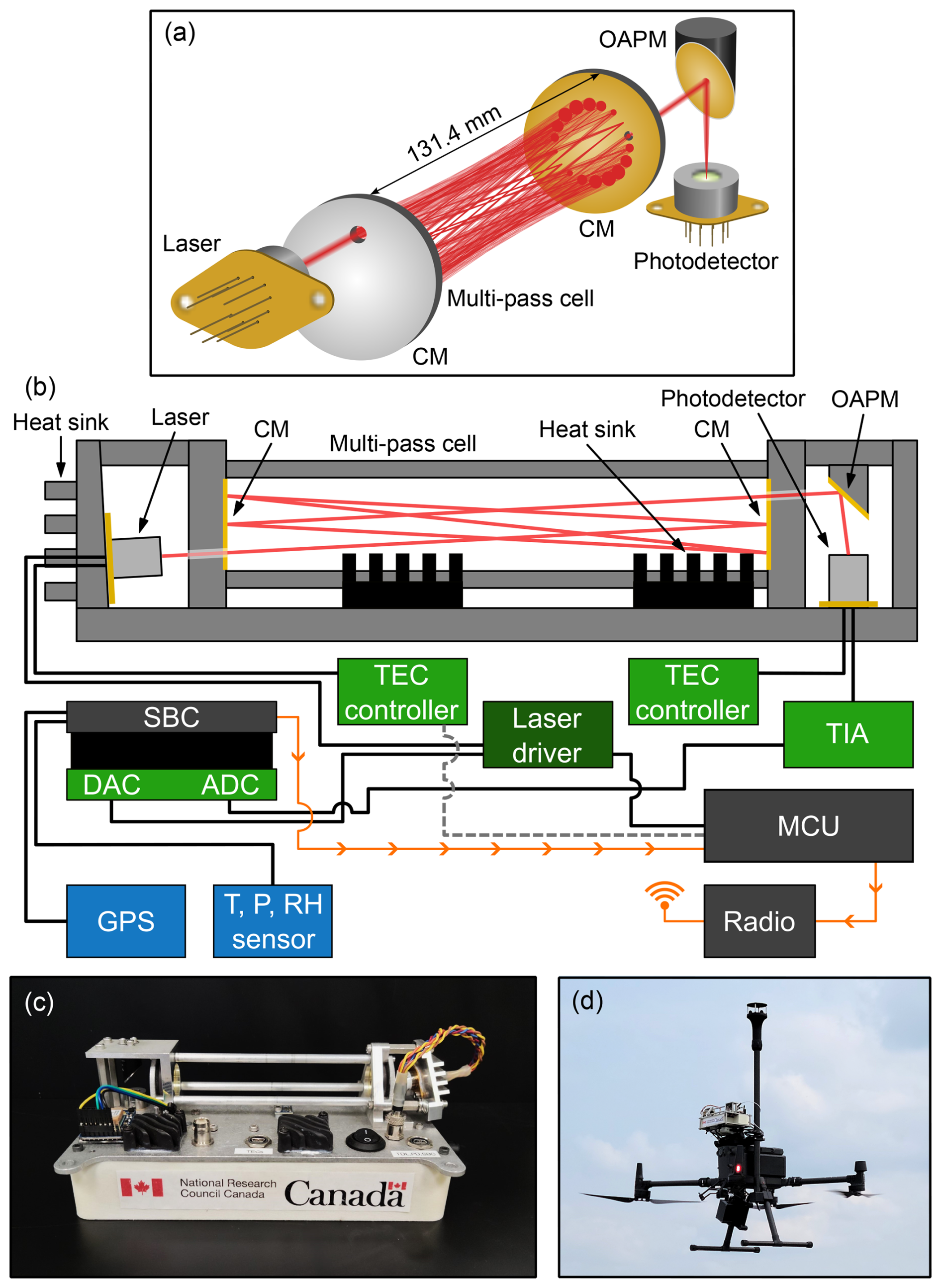
Figure 1 (a) Schematic of methane sensor optical head showing laser beam trajectory. (b) Schematic showing sensor components and electrical connections. For clarity, the power supply is not shown. CM: concave mirror; OAPM: off-axis parabolic mirror; SBC: single board computer; DAC: digital-to-analog converter; ADC: analog-to-digital converter; TEC: thermoelectric cooler; TIA: transimpedance amplifier; MCU: microcontroller unit. (c) Close up of the ultra-lightweight methane sensor. (d) Sensor and Gill WindUltra anemometer deployed on a DJI Matrice 300 RTK UAV.

The laser beam exiting the multi-pass cell is directed and focused onto an optically-immersed HgCdTe photovoltaic detector (PVI-2TE-4-0.1x0.1-TO66-wAl2O3-70, Vigo Photonics, Poland) using an off-axis parabolic mirror (OAPM) (MPD01M9-M01, Thorlabs, USA).

The laser, its heat sink, both mirrors of the multi-pass cell, and the OAPM are integrated into a rigid, cage-like assembly that reduces the effects of mechanical vibrations during UAV flight deployments (see Fig. 1c). Laser pre-alignment is achieved using a mounting plate machined at the desired injection angle. The optical alignment is fine-tuned during the assembly procedure using shims and split lock washers to correct deviations in the laser pointing angle. The split lock washers provide small angular adjustment capability, while slightly over-sized mounting holes for the laser heat sink and OAPM allow limited translational freedom. Final alignment was achieved by measuring the laser pointing angle, applying the required corrections, and making small translational and angular adjustments to maximize the detector signal observed on an oscilloscope. The number and approximate positions of the reflected spots are confirmed by systematically blocking the laser beam at the face of one mirror and monitoring the detector response.

2.2 Temperature control and power consumption

Both the laser and the photodetector are temperature-stabilized via integrated thermoelectric coolers (TECs), controlled by ultra-stable TEC controllers (WTC32ND, Wavelength Electronics, USA). The laser is mounted on a custom aluminum heatsink affixed to the multi-pass optical cell. The photodetector is mounted directly to the sensor's aluminum baseplate, which also dissipates heat. The TEC controllers are mounted on custom-designed printed circuit boards (PCBs), which were adapted from the manufacturer’s evaluation board (WTC32ND-EV, Wavelength Electronics, USA) with added fail-safe protection circuitry to prevent accidental thermal runaway events. Heatsinks affixed to the aluminum baseplate directly opposite the TEC controllers dissipate heat generated by the TEC drive currents. The laser temperature is regulated to an average of 7.3 °C, while the detector is cooled to −42.7 °C. Under active airflow, the temperatures of both laser and detector typically stabilize within 10 min. A similar stabilization period is required after rapid, substantial changes in ambient temperature. During UAV flight, the laser temperature is maintained to within ±0.1 °C, which corresponds to a wavelength stability of ±0.028 nm (±0.026 cm⁻¹).

The sensor is powered by a 5 VDC supply delivered through two mini type-B USB ports, which can be conveniently driven by a standard power pack with dual type-A USB outputs that each provide a minimum 2 A current output to sustain the TEC operation on startup. At room temperatures and in steady-state, the sensor package (including the SBC) consumes around 11 W of electrical power. For comparison, the previous version of this TDLAS methane sensor had a steady state power draw of around 18 W (Norooz Oliaee et al., 2022). More than half of the power draw is attributed to the two TECs and their controllers, with the photodetector TEC being the dominant consumer. At colder air temperatures, the overall power consumption decreases due to the reduced load on the photodetector TEC.

2.3 Onboard signal generation, acquisition, and processing

A schematic of the electrical interconnections is shown in Fig. 1b. Signal generation and processing is handled onboard and in real time using a low-cost BeagleBone Black SBC (BeagleBoard.org, USA). The SBC is furnished with a custom PCB that houses a 12-bit digital-to-analog converter (DAC; AD5621, Analog Devices, USA) and a 16-bit analog-to-digital converter (ADC; MCP33131D-10, Microchip, USA). For reference, the DAC and ADC have simple passive RC filters at their input and output with 3 dB bandwidths of 32.8 and 48.2 kHz, respectively. The DAC and ADC are interfaced with the SBC via two 32-bit 200 MHz on-chip programmable real-time units (PRUs) and a memory buffer, which enables data transfer rates to be independent of the Linux operating system processes.

The DAC translates digital modulation patterns computed numerically by the SBC to analog voltages at a sampling rate of 400 kHz. This analog signal is fed to a low noise laser diode driver (DRV200-A-200, Koheron, France) as modulation input. The driver simultaneously provides a constant DC offset current, enabling the central laser wavelength to be tuned to the methane absorption line at 3270.4 nm (Dang-Nhu et al., 1979; Gordon et al., 2026). The laser injection current is swept from 110 to 200 mA in a sawtooth pattern with a frequency of 100 Hz, producing a corresponding wavelength sweep rate of approximately 20 pm mA⁻¹ near the target wavelength. A sinusoidal modulation with a frequency of 10 kHz and a peak amplitude of 15 mA is added to the current ramp for the purpose of noise rejection by wavelength modulation and subsequent lock-in detection. The amplitude of the modulation signal was chosen empirically to increase the second harmonic signal amplitude while avoiding excessive over-modulation and does not reflect the well-known optimum modulation index (m≈2.2) (Rieker et al., 2009; Reid and Labrie, 1981).

The photocurrent signal from the photodetector is converted to a voltage using a custom two-stage transimpedance amplifier (TIA) with a 3 dB bandwidth of 141 kHz. The analog voltage signal from the TIA is acquired by the ADC at a sampling rate of 312.5 kHz. The SBC computes the second harmonic (2f) spectrum, X_2f(t), from the raw time-dependent detector signal, I_t(t), by applying a digital lock-in amplifier:

$$\begin{array}{}\text{(1)}& X_{\mathrm{2}f}\left(t\right)=\mathrm{LP}\mathit{\left\{}{I}_t\right(t)\times \cos (\mathrm{2}\mathit{\pi }t\cdot \mathrm{2}f+\mathit{\varphi }\left)\mathit{\right\}}\end{array}$$

where t is time, f is the modulation frequency, ϕ is the detection phase, and LP is a digital low-pass filter. For the latter, a numerical fourth-order low-pass filter with a −3 dB cutoff frequency of 561 Hz is applied, implemented as two cascaded second-order biquad sections, each with a cutoff frequency of 700 Hz. The detection phase is selected empirically to maximize the magnitude of the methane peak in the second harmonic spectrum, X_2f. The amplitude of the methane peak is computed using a simple search algorithm to find the methane peak and left-side trough in the 2f spectrum by looking for the minimum and maximum values within predefined bounds. The peak-to-peak amplitude is used to compute the methane mole fraction by calibrating to reference gas mole fractions, as described in Sect. 3.1.

The SBC records the computed methane mole fraction as a function of time at a rate of 100 Hz along with ambient temperature, pressure, and relative humidity data, which are measured by an onboard sensor (BME280, Bosch Sensortec, Germany). A GPS module (Ultimate GPS, Adafruit, USA) is used to timestamp the data relative to coordinated universal time (UTC). The SBC saves all timestamped data to a microSD card. Optionally, raw data files containing the detector signal and the 2f spectrum can also be saved.

In addition to the data saved locally at 100 Hz, a down-sampled and averaged data stream with a rate of 5 Hz is passed over a universal asynchronous receiver-transmitter (UART) connection to a microcontroller unit (MCU; Metro Mini, Adafruit Industries, USA), which acts as a data hub. The MCU board also monitors the laser temperature, acting as a digital interlock that shuts off the laser driver if the laser temperature is not within pre-defined bounds. The MCU optionally feeds the down-sampled methane mole fraction, laser temperature, and ambient conditions data into a high-powered radio modem (RFD900x, RF Design, Australia), enabling long-distance real-time monitoring of the data stream while the sensor is deployed on a UAV. Although the data transmitted over the wireless link is not used for processing or analysis, real-time monitoring of mole fraction data is invaluable for guiding flight missions in the field and also for system health monitoring.

2.4 Mechanical assembly

The optical assembly, photodetector, and electronic components are affixed to an aluminum baseplate. The sensor package is compact and easily portable, with outer dimensions of 23.5 cm (L) × 12.5 cm (W) × 9.5 cm (H), approximately 84 % smaller than the prior instrument (Norooz Oliaee et al., 2022). Including all electronics, batteries, and peripheral devices such as ambient condition (pressure, temperature, and relative humidity) sensors and a GPS receiver, the mass of the sensor package is just 1.2 kg, roughly one quarter that of its 5 kg predecessor (Norooz Oliaee et al., 2022). As one of the lightest methane gas spectrometers developed to date, the instrument is well within the payload limits of many small consumer- or enterprise-grade UAVs such as the DJI Matrice 300 RTK used in this study, allowing for simultaneous deployment of an on-board anemometer system on a highly portable measurement platform, as described in Sect. 2.5.

2.5 UAV integration

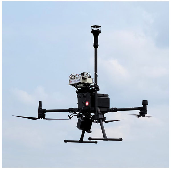
We deploy the 1.2 kg sensor system on a DJI Matrice 300 RTK UAV (DJI, China) that has a mass of 6.3 kg (including batteries) and a maximum payload of 2.7 kg, as shown in Fig. 1d. The instrument is secured to the top of the UAV using a modified DJI upward gimbal connector, providing vibration isolation. With the sensor onboard, we have achieved UAV flight times up to 28 min, limited by the UAV batteries. The methane sensor itself is powered independently from the UAV using a 10 000 mAh power bank (Adafruit, USA), enabling continuous operation for over 2 h and allowing multiple sequential UAV flights without shutting down the sensor.

Flight mission trajectories are pre-programmed and transferred to the flight controller before starting each mission to achieve systematic flight patterns. During flight, the UAV travels at a constant speed in the range of 5 to 8 m s⁻¹ along each horizontal transect and comes to a stop before changing altitude or direction.

We have deployed the sensor and UAV system at altitudes from approximately 0.5 to 40 m above takeoff, and we expect that higher flight altitudes would be achievable. In Canada, the maximum legal flight altitude is 122 m above ground level, for most UAV operations (Canadian Aviation Regulations, SOR96/433, s901.25, Government of Canada, 2026).

2.6 Onboard wind measurements

The requirement for onboard wind measurements is determined by the mission goals and data analysis methods. For emission flux quantification missions, onboard wind data is highly beneficial. For hot spot and leak detection applications, an onboard anemometer may be unnecessary if the general wind direction is known from local weather stations or models.

When measuring onboard wind, a 2D anemometer (WindUltra, Gill Instruments, UK) is affixed to the UAV, enabling simultaneous measurement of methane mole fraction and wind information. The anemometer is mounted on a carbon fiber mast approximately 37 cm above the sensor’s optical head and 75 cm above the UAV rotors, reducing the effect of rotor wash on the recorded wind measurements. Custom 3D-printed components secure the mast and a data logger for the anemometer to the UAV landing gear. The entire anemometer assembly including the anemometer head, mast, data logger, and battery add an additional 1.2 kg to the payload. Together, the methane sensor and anemometer systems make up a total UAV payload of 2.4 kg. With the entire payload, including the methane sensor and anemometer components, the DJI Matrice 300 RTK UAV can achieve flight times of approximately 20 min.

The anemometer is mounted with the “north” direction pointing to the front of the UAV and the front of the aircraft is always oriented in the direction of flight, such that onboard wind is recorded relative to the direction of travel. To recover the true wind speed and direction (u,θ) from those measured by the onboard anemometer (u_anem,θ_anem), we must account for the movement of the UAV, including its horizontal ground speed v_gnd, pitch angle Θ_pitch, and roll angle Φ_roll. The corrected wind speed components parallel, u_∥, and perpendicular, u_⟂, to the UAV flight direction are given by:

$$\begin{array}{}\text{(2)}& u_{\parallel }={\displaystyle \frac{u_{\mathrm{anem}}\cos \left({\mathit{\theta }}_{\mathrm{anem}}\right)}{\cos \left({\mathrm{\Theta }}_{\mathrm{pitch}}\right)}}-v_{\mathrm{gnd}},u_{⟂}={\displaystyle \frac{u_{\mathrm{anem}}\sin \left({\mathit{\theta }}_{\mathrm{anem}}\right)}{\cos \left({\mathrm{\Phi }}_{\mathrm{roll}}\right)}}\end{array}$$

The pitch and roll angle corrections compensate for the 2D anemometer’s measurement axes being tilted from horizontal when the UAV is in flight. We apply a cosine correction and assume that the vertical wind speed is negligible compared to the horizontal wind. The corrected wind speed and direction are given by:

$$\begin{array}{}\text{(3)}& u=\sqrt{u_{\parallel }^{\mathrm{2}}+u_{⟂}^{\mathrm{2}}},\mathit{\theta }=\mathrm{atan}\mathrm{2}(u_{⟂},u_{\parallel })+\mathit{\psi }\end{array}$$

where atan2 is the four-quadrant inverse tangent and ψ is the UAV heading relative to north.

2.7 Emission flux quantification

To quantify methane emission flux, we apply a direct flux quantification method that relies on the principle of mass balance (Scheutz et al., 2025; Dooley et al., 2024; Bonne et al., 2024). In this method, the UAV flies a pattern known as a “flux curtain” downwind of the methane source, consisting of stacked horizontal transects that form a vertical plane (Scheutz et al., 2025; Dooley et al., 2024; Bonne et al., 2024; Morales et al., 2022; Andersen et al., 2021; Shah et al., 2020). The lateral extent of the flux curtain is chosen to ensure that the UAV traverses the entire width of the plume in each transect. The curtain height is also dictated by the size and shape of the plume, such that elevated methane mole fractions are not observed in the upper two to three transects. The vertical spacing between successive transects is minimized to give the best possible vertical resolution within the constraints of limited flight duration. The result is a two-dimensional map of the methane plume over a vertical plane downwind of the source.

Methane mole fractions ${\mathit{\chi }}_{{\mathrm{CH}}_{\mathrm{4}}}$ are recorded by the sensor at a rate of 100 Hz throughout the flight. They are converted to dry mole fractions using the relation ${\mathit{\chi }}_{{\mathrm{CH}}_{\mathrm{4}}}^{\mathrm{dry}}={\mathit{\chi }}_{{\mathrm{CH}}_{\mathrm{4}}}/(\mathrm{1}-{\mathit{\chi }}_{{\mathrm{H}}_{\mathrm{2}}\mathrm{O}})$, where ${\mathit{\chi }}_{{\mathrm{H}}_{\mathrm{2}}\mathrm{O}}$ is the water vapor mole fraction. In post-processing, a 0.1 s moving average is applied and the data is down-sampled to match the 10 Hz positional data stream from the UAV flight logs. The wind speed and direction are also recorded at a rate of 10 Hz. For each measurement point in the y-z flux curtain, the methane flux density is given by:

$$\begin{array}{}\text{(4)}& \begin{array}{rl}q(y,z)& =\left({\mathit{\chi }}_{{\mathrm{CH}}_{\mathrm{4}}}^{\mathrm{dry}}(y,z)-{\mathit{\chi }}_{{\mathrm{CH}}_{\mathrm{4}}}^{\mathrm{bkg},\mathrm{dry}}(y,z)\right)(\mathrm{1}-{\mathit{\chi }}_{{\mathrm{H}}_{\mathrm{2}}\mathrm{O}}(y,z\left)\right)\\ & \cdot u_x(y,z)\cdot p\left(z\right){\displaystyle \frac{M_{{\mathrm{CH}}_{\mathrm{4}}}}{RT}}\end{array}\end{array}$$

where ${\mathit{\chi }}_{{\mathrm{CH}}_{\mathrm{4}}}^{\mathrm{bkg},\mathrm{dry}}$ is the background methane dry mole fraction, u_x is the wind speed component orthogonal to the y-z flux curtain, p(z) is the pressure at altitude z, $M_{{\mathrm{CH}}_{\mathrm{4}}}=\mathrm{16.04}$ g mol⁻¹ is the molar mass of methane, R is the gas constant, and T is the average temperature. The pressure p(z) is estimated by applying a linear fit to the data recorded by the onboard pressure sensor throughout the flight. In this work, equivalent ${\mathit{\chi }}_{{\mathrm{H}}_{\mathrm{2}}\mathrm{O}}$ values were used for both the measured and background dry mole fractions ${\mathit{\chi }}_{{\mathrm{CH}}_{\mathrm{4}}}^{\mathrm{dry}}$ and ${\mathit{\chi }}_{{\mathrm{CH}}_{\mathrm{4}}}^{\mathrm{bkg},\mathrm{dry}}$ such that Eq. (4) simplifies to:

$$\begin{array}{}\text{(5)}& q(y,z)=\left({\mathit{\chi }}_{{\mathrm{CH}}_{\mathrm{4}}}\right(y,z)-{\mathit{\chi }}_{{\mathrm{CH}}_{\mathrm{4}}}^{\mathrm{bkg}}(y,z\left)\right)\cdot u_x(y,z)\cdot p\left(z\right){\displaystyle \frac{M_{{\mathrm{CH}}_{\mathrm{4}}}}{RT}}\end{array}$$

For each horizontal transect, a transect-integrated flux density ${\int }_{\mathrm{tr}.}q\mathrm{d}y$ is calculated using the trapezoid rule for numerical integration. The total flux Q is determined by integrating over the transect-integrated flux density in the vertical direction from ground level (z=0) to the top of the flux curtain.

$$\begin{array}{}\text{(6)}& Q=\underset{\mathrm{0}}{\overset{z_{\max }}{\int }}\underset{\mathrm{tr}.}{\int }q(y,z)\mathrm{d}y\mathrm{d}z\end{array}$$

where z_max is the altitude of the highest transect in the flux curtain, which should ideally exceed the vertical extent of the emission plume such that the transect-integrated flux density of the uppermost transect is zero. As such, no extrapolation is required above the flux curtain. On the other hand, plume dynamics and operational constraints often lead to non-zero flux densities in the lowest measured transect, necessitating extrapolation from the lowest transect to the ground. In this work, we define “extrapolated” transects below the measured flux curtain and predict corresponding transect-integrated flux densities using a logarithmic wind model to generate extrapolated wind speeds and assuming a constant transect-integrated methane mole fraction ${\int }_{\mathrm{tr}.}{\mathit{\chi }}_{{\mathrm{CH}}_{\mathrm{4}}}\mathrm{d}y$ from the lowest transect to the ground. We assigned a relatively large uncertainty bound to the quantity ${\int }_{\mathrm{tr}.}{\mathit{\chi }}_{{\mathrm{CH}}_{\mathrm{4}}}\mathrm{d}y$ for the extrapolated transects, following a normal distribution for which the probability that ${\int }_{\mathrm{tr}.}{\mathit{\chi }}_{{\mathrm{CH}}_{\mathrm{4}}}\mathrm{d}y>\mathrm{0}$ ppm m is 99 %. The logarithmic wind model is given by

$$\begin{array}{}\text{(7)}& u\left(z\right)={\displaystyle \frac{u^{*}}{\mathit{\kappa }}}\ln \left({\displaystyle \frac{z}{z_{\mathrm{0}}}}\right)\end{array}$$

where u^* is the friction velocity, z₀ is the surface roughness, and κ=0.4 (Visscher, 2014; Bolek et al., 2024, 2026). The model is fit to altitude-dependent wind data recorded from the UAV. The corresponding 1σ prediction interval is included in the uncertainty estimates for the transect-integrated flux density for the extrapolated transects.

Following the trapezoid rule, linear interpolation is used when integrating between transects – both measured and extrapolated – in Eq. (6). This direct interpolation approach is suited to datasets characterized by dense sampling across the measurement plane (Bonne et al., 2024; Bolek et al., 2026; Scheutz et al., 2025; Dooley et al., 2024). More complex statistical interpolation approaches such as Kriging have also been proposed (Morales et al., 2022; Andersen et al., 2021), and may be more suitable than direct interpolation for sparse datasets.

Uncertainties in methane mole fraction, wind speed, and methane density are propagated when evaluating the uncertainty on total flux Q. We also estimate the extrapolation uncertainty, as described above, and the interpolation uncertainty using leave-one-out cross-validation. Details regarding the error propagation can be found in the Appendix.

3 Results and discussion

3.1 Sensor calibration and performance

The laser injection current over time is shown in Fig. 2a and the resultant detector signal is shown in Fig. 2b, for ambient air with a methane mole fraction near 2 ppm. The corresponding second harmonic spectrum is shown in Fig. 2c. The 3270.4 nm absorption feature for methane is indicated, along with a nearby water absorption line centered at 3271.0 nm. At the time of measurement, the ambient temperature was 22.6 °C and the relative humidity was 51.5 %, yielding a water vapor mole fraction of approximately 1.4 %. The feature contained within the shaded region of Fig. 2c is produced by the response of the filtering function to the abrupt change in the photodetector signal from the previous laser sweep and is not indicative of light absorption.

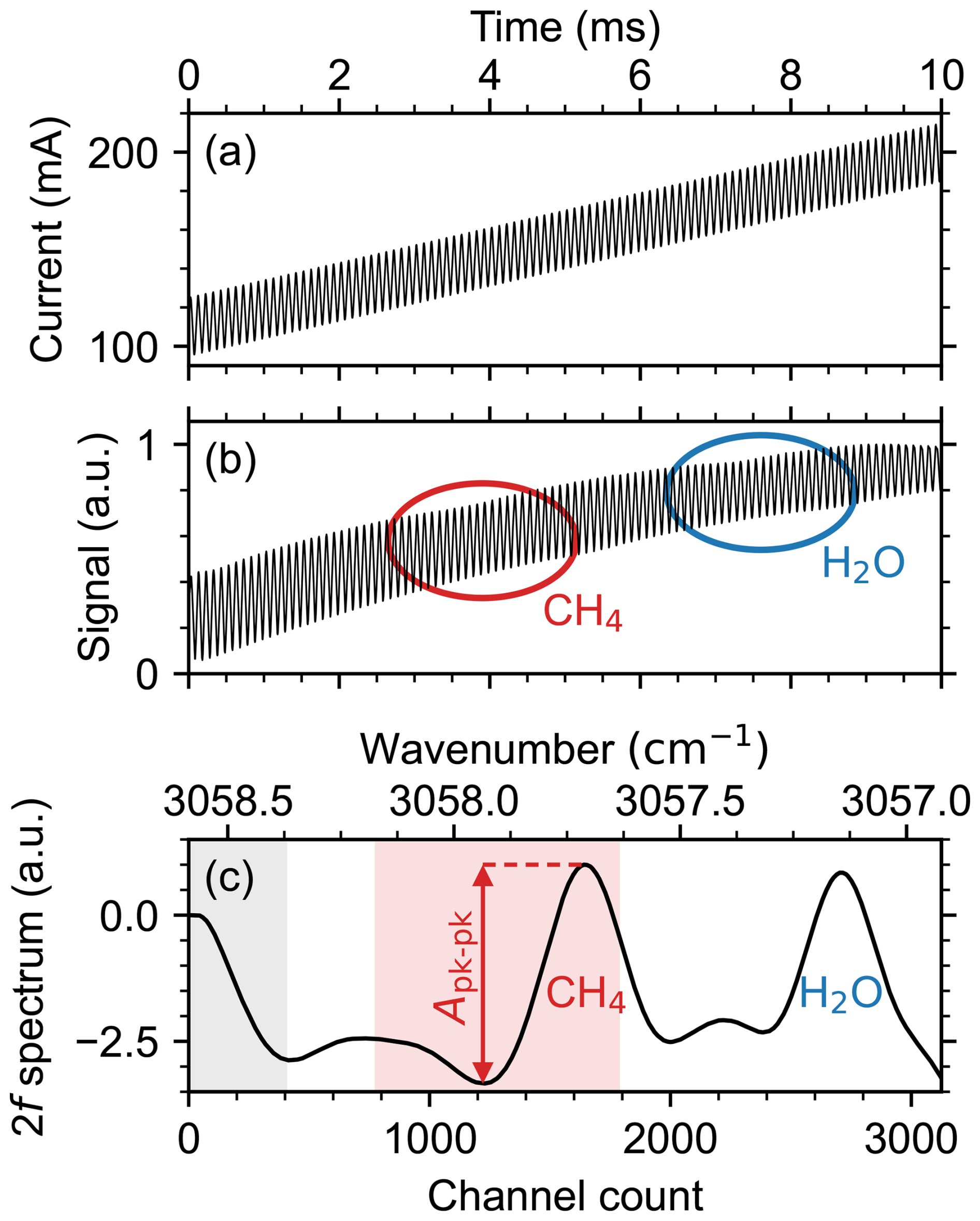
Figure 2 (a) Laser injection current ramp and 10 kHz modulation over one sawtooth period. (b) Corresponding normalized detector signal observed under ambient measurement conditions. (c) Demodulated second harmonic spectrum, normalized. Absorption features due to CH₄ and H₂O are indicated in (b, c). The gray shaded region in (c) spanning channels 0 to 400 contains the initial response of the low pass filter and does not indicate absorption. The red shaded region covering the CH₄ peak indicates the predefined bounds used to identify the peak-to-peak amplitude.

We calibrated the sensor in an enclosed chamber with a volume of approximately 50 L under controlled gas flow conditions with a known mole fraction. The temperature within the enclosure was maintained at 21 °C using a heat exchanger. Calibration gas mixtures with mole fractions ranging from 2 to 50 ppm were generated using in-line mass flow controllers (MFCs) to combine pre-mixed methane-in-air gas cylinders (AirLiquide, Canada) with synthetic air. The calibration gas flow was maintained near 10 L min⁻¹. A LI-7810 trace gas analyzer (LI-COR Environmental, USA) was used as a reference instrument to benchmark the methane mole fraction. We assign a 1 % uncertainty to the mole fractions recorded by the LI-7810.

For each calibration step, the flow was established and the mole fraction was allowed to stabilize before progressing to the next step. The peak-to-peak amplitude of the methane feature in the WMS 2f spectrum is used for mole fraction calibration. The response of the sensor as a function of methane mole fraction is shown in Fig. 3. The response of the sensor to increasing methane mole fraction is nearly linear up to 10 ppm; however, further increase in the calibration gas mole fraction can be described by a higher order polynomial, as previously reported in Norooz Oliaee et al. (2022). Here, the non-linear calibration curve corresponds to a fourth order polynomial such that

$$\begin{array}{}\text{(8)}& \begin{array}{rl}{\mathit{\chi }}_{{\mathrm{CH}}_{\mathrm{4}}}^{\mathrm{dry}}\left(A_{\mathrm{pk}-\mathrm{pk}}\right)& =a_{\mathrm{4}}{A}_{\mathrm{pk}-\mathrm{pk}}^{\mathrm{4}}+a_{\mathrm{3}}{A}_{\mathrm{pk}-\mathrm{pk}}^{\mathrm{3}}+a_{\mathrm{2}}{A}_{\mathrm{pk}-\mathrm{pk}}^{\mathrm{2}}\\ & +a_{\mathrm{1}}{A}_{\mathrm{pk}-\mathrm{pk}}+a_{\mathrm{0}}\end{array}\end{array}$$

where A_pk−pk is the WMS 2f peak-to-peak amplitude and the variables a_i are fitting parameters. The fit parameters are obtained by orthogonal distance regression. The resultant calibration parameters for the curve shown in Fig. 3a are $a_{\mathrm{4}}=\mathrm{1540}\pm \mathrm{170}$ ppm, $a_{\mathrm{3}}=-\mathrm{717}\pm \mathrm{114}$ ppm, $a_{\mathrm{2}}=\mathrm{163}\pm \mathrm{22}$ ppm, $a_{\mathrm{1}}=\mathrm{88.9}\pm \mathrm{1.4}$ ppm, $a_{\mathrm{0}}=-\mathrm{0.095}\pm \mathrm{0.024}$ ppm, where the uncertainties are reported to one standard deviation. Figure 3b shows the relative residuals together with the 1σ standard error on the fit and the 95 % confidence interval. Over the range of 1.8 to 55 ppm, the 1σ bounds lie within 1.5 % of the fit.

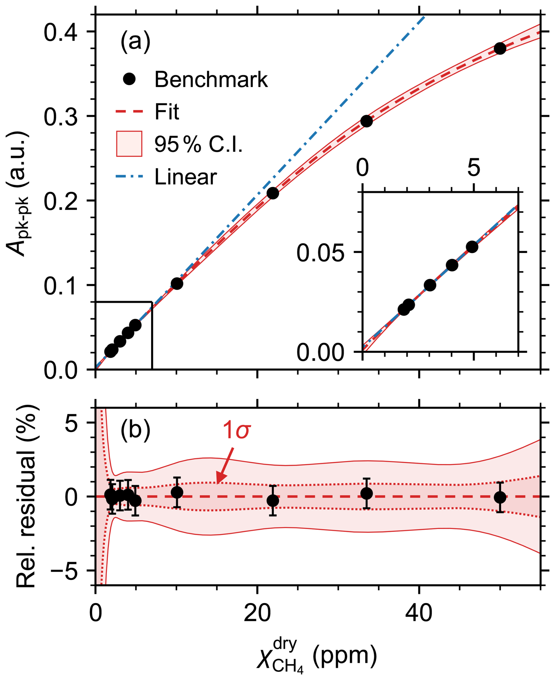
Figure 3 (a) WMS 2f peak-to-peak amplitude as a function of methane mole fraction measured by benchmark instrument (LI-7810). Fit to Eq. (8) is shown with 95 % confidence interval. For reference, a linear fit to the data points below 10 ppm is also shown. Inset shows expanded view of data points up to 5 ppm. (b) Relative residuals $({\mathit{\chi }}_{{\mathrm{CH}}_{\mathrm{4}}}^{\mathrm{dry}}-{\mathit{\chi }}_{{\mathrm{CH}}_{\mathrm{4}}}^{\mathrm{fit}})/{\mathit{\chi }}_{{\mathrm{CH}}_{\mathrm{4}}}^{\mathrm{fit}}$, where error bars indicate 1 % uncertainties on the methane mole fraction. The 1σ standard error on the fit is also shown.

We performed a measurement of the Allan-Werle variance in the calibration enclosure for a duration of 2 h using the 2.00 ppm methane-in-air calibration gas to determine the stability and precision of the sensor (Fig. 4). For comparison, we generated a second Allan-Werle deviation plot using in-flight data from a period when the sensor was measuring background methane concentrations during a controlled-release experiment. The UAV flew a “curtain-type” flight pattern with horizontal transects at altitudes ranging from 0 to 30 m above ground level. The average wind speed during the flight period was 2.5 m s⁻¹ with a standard deviation of 0.7 m s⁻¹. The temperature was around 22.5 °C, the pressure at ground level was 1005 hPa, and the relative humidity was 65 %. The in-flight dataset only extends up to an integration time of approximately 300 s due to the limited flight duration.

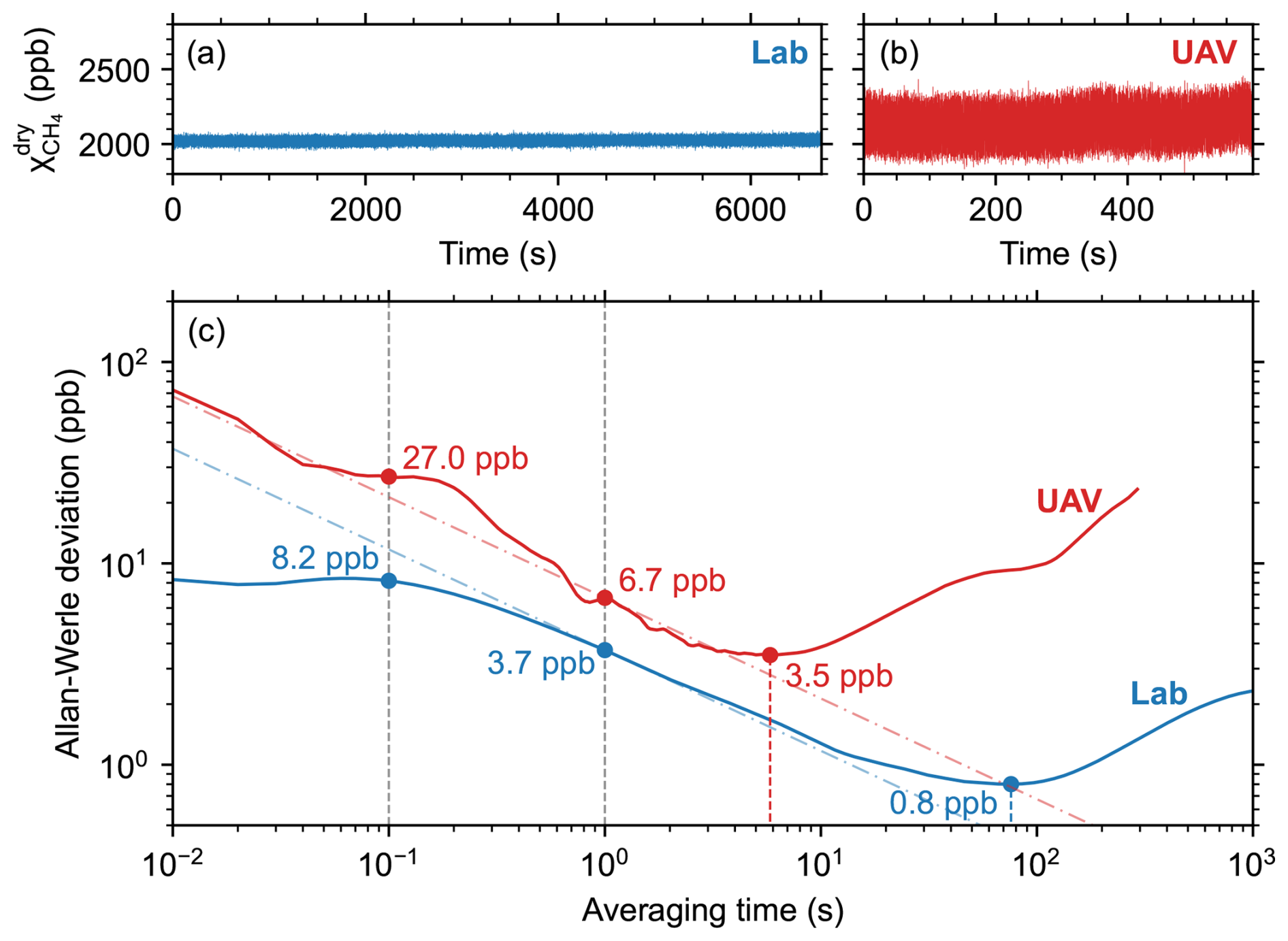
Figure 4 (a, b) Methane dry mole fraction 100 Hz timeseries (a) in laboratory enclosure and (b) during UAV flight. (c) Overlapping Allan-Werle deviation plots generated from the laboratory and in-flight timeseries. Dash-dot lines indicate $\sqrt{\mathrm{1}/\mathit{\tau }}$ white noise behavior where τ is the averaging time (Werle, 2011).

For reference, $\sqrt{\mathrm{1}/\mathit{\tau }}$ white noise behavior (Werle, 2011) is indicated by the dash-dot lines in Fig. 4. Additional noise observed in-flight is primarily caused by inductive noise from the high-powered radio module used for real-time monitoring of mole fraction and telemetry data during flight. Though not required in all scenarios, real-time monitoring is frequently used to enable on-the-fly modification of the mission plan based on the observed methane mole fractions. It may be possible to reduce this noise component by implementing design modifications such as a Faraday cage to mitigate electromagnetic interferences.

The in-lab Allan-Werle deviation below 0.1 s averaging time is affected by a quasi-periodic noise signature for which averaging does not initially improve the measurement precision, appearing as random-walk or correlated noise in the Allan-Werle plot. Though the root cause is still under investigation, the effect is likely induced by correlated mechanical or electrical noise (Röder et al., 2024; Gan et al., 2026). For the in-flight data, there is a deviation from the $\sqrt{\mathrm{1}/\mathit{\tau }}$ white noise behavior observed for averaging times between 0.1 and 1 s that may be due to optical fringe effects that are not observed in the laboratory data (Werle, 2011).

The Allan-Werle plot demonstrates that, by averaging the sensor’s in-flight and laboratory mole fraction data up to 5.8 and 75.9 s, respectively, corresponding optimum precisions of 3.5 and 0.8 ppb are achieved. In both cases, sensor drift dominates precision beyond the optimal averaging times. In the laboratory, the test was performed in a temperature-controlled calibration enclosure, but gradual changes in pressure likely contributed to the drift. For the in-flight test, environmental conditions were not controlled and the sensor experienced rapid changes in air flow as the UAV changed directions. As a result, drift dominates the sensor behavior at shorter averaging times during flight compared with laboratory conditions.

The 1 s averaging times (in-flight precision: 6.7 ppb; laboratory precision: 3.7 ppb) represent a useful metric for comparison to other lightweight UAV sensors. Though other instruments offer slightly smaller 1 s precisions in the range of 1–5 ppb, to our knowledge the ultra-lightweight sensor presented here offers the best 1 s precision for a sub-2 kg methane sensor reported to date. For an open-path system on a mobile platform moving at 5 to 8 m s⁻¹, longer averaging times (>1 s) can result in smearing and loss of information. The averaging time that we use in this study is 0.1 s, corresponding to an in-flight precision of 27 ppb.

3.2 Sensitivity to changing environmental conditions

Due to its open-path design, the sensor is subject to changes in ambient temperature, pressure, and relative humidity, which directly impact the measured absorption spectrum. Ideally, the sensor should be calibrated under laboratory conditions that are similar to deployment conditions, and the effects of variation in those conditions should be considered in the measurement uncertainty budget.

The ambient air temperature affects the sensor response in several different ways. First, there is the impact of temperature on optical absorbance, wherein the absorbance will decrease with increasing temperature, for the absorption lines employed in this study. Thermal expansion and contraction in the mechanical assembly may impact the effective path length and optical alignment of the multi-pass cell. Rapid temperature changes can also disrupt the thermal stability of the laser and photodetector.

The relative change in methane mole fraction recorded by the sensor at different temperatures in the range of 21 to 29 °C is shown in Fig. 5. At each temperature, the methane mole fraction was varied in the range of 2 to 50 ppm, using the LI-7810 trace gas analyzer as a reference instrument. At each temperature setpoint, the sensor was allowed to stabilize under active airflow, and temperature stability within the enclosure was maintained to within 0.3 °C. The mole fractions recorded by the reference sensor, which was connected to the calibration chamber by a gas line but was not itself contained within the enclosure, were stable to within 0.6 %. Compared to the mole fractions recorded by the ultra-lightweight sensor at the calibration temperature (20.9 °C), the average recorded mole fraction drops by 3.5 % at 24.6 °C, and by 4.8 % at 28.7 °C. For comparison, the expected change in peak methane absorbance when the temperature increases by 7.8 °C is −4.6 %, or a change in optical absorption of −4.5 % at 2 ppm and −2.3 % at 50 ppm (Goldenstein et al., 2017; Gordon et al., 2026). The impact of temperature-dependent absorbance could potentially be mitigated by selecting a different methane absorption line (Li et al., 2020), though there may be associated trade-offs such as reduced line strength and more limited commercial availability of lasers.

In this work, we have accounted for the sensor's temperature dependence primarily within the measurement uncertainty. Further study into the sensor's non-linear temperature-dependent response is needed to facilitate the implementation of a robust correction protocol. Modifications to the sensor optical head using materials with a lower coefficient of thermal expansion may help to mitigate temperature-dependent effects that are mechanical in nature. The implementation of a $\mathrm{2}f/\mathrm{1}f$ normalization routine (Rieker et al., 2009) may also improve tolerance to misalignments and reduce associated temperature-effects. Though $\mathrm{2}f/\mathrm{1}f$ normalization is more computationally demanding than the 2f calculation used in this work, we expect that it could be implemented with the same hardware by optimizing resource allocations on the single board computer.

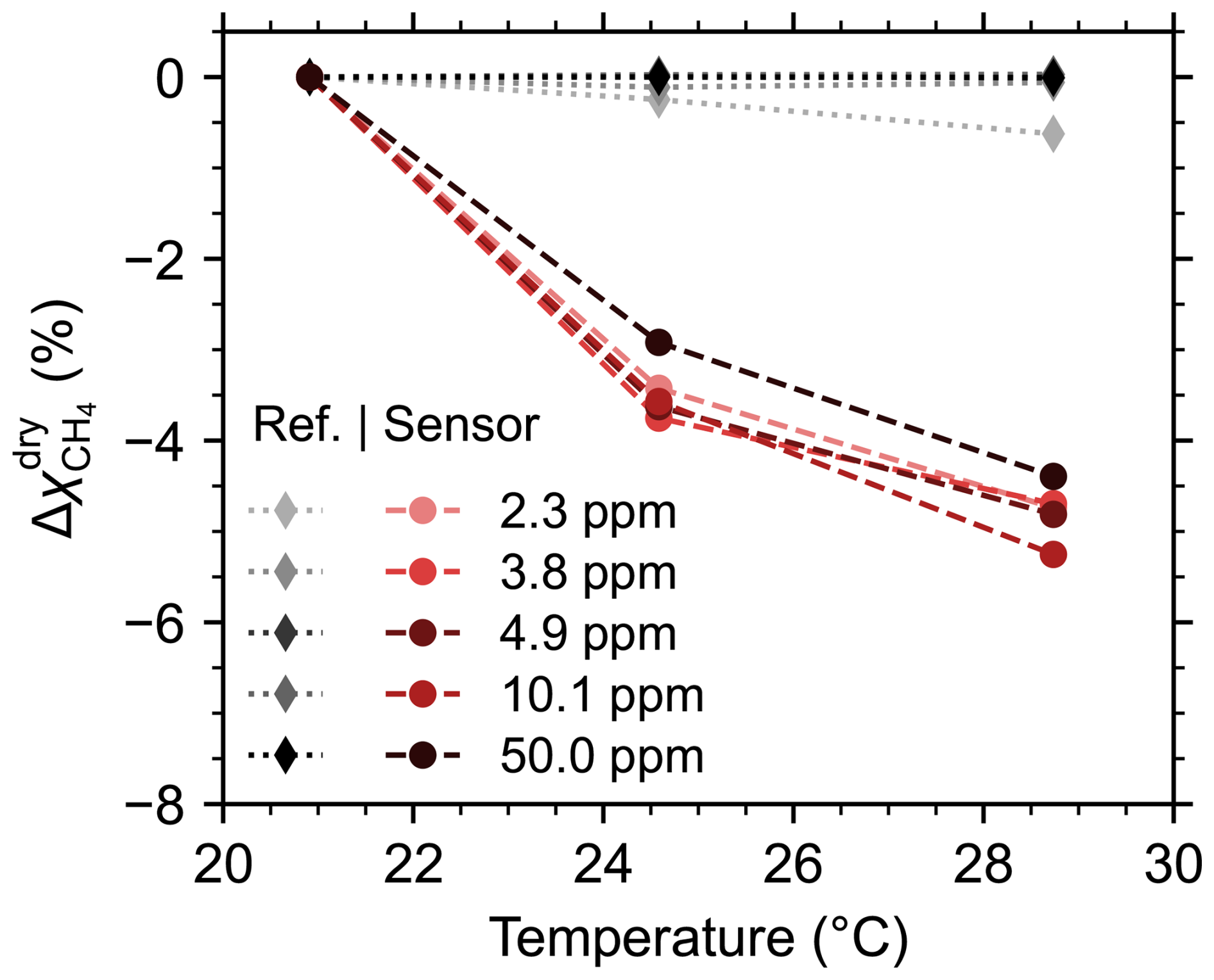
Figure 5 Relative change in the methane dry mole fraction recorded by the sensor versus temperature. The response of the reference instrument is shown for comparison.

Although the TECs that control the temperatures of the laser and photodetector can adapt to gradual variations in ambient temperature and maintain stable performance across a wide temperature range, sudden shifts in ambient temperature may cause temporary instability. The impact of rapid changes in temperature in the range of 19.7 to 27.5 °C is shown in Fig. 6. The timeseries data corresponds to the native 100 Hz sensor output. To clearly illustrate the effect of the rapid temperature variation, the 60 s moving average is also shown, indicated by the black dashed line. Oscillatory behavior is observed in the sensor signal immediately after each abrupt temperature change. Over the entire experiment, the 60 s moving average varies by 4.1 %.

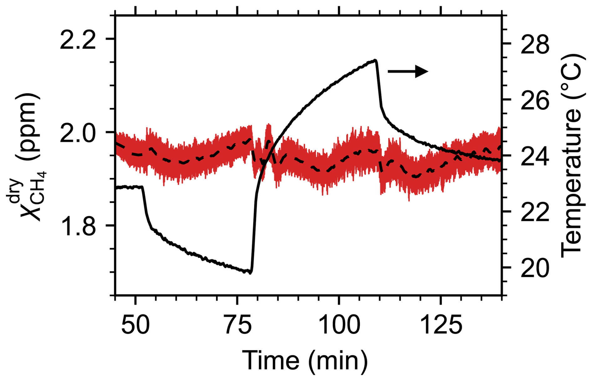
Figure 6 100 Hz time series for the recorded methane dry mole fraction while the temperature of the calibration enclosure was rapidly varied (red). The dashed line indicates the 60 s moving average. Temperature is shown on the right-hand axis.

Methane absorbance at 3270.4 nm changes with pressure at a rate of about 0.033 % per hPa (Goldenstein et al., 2017; Gordon et al., 2026). When deployed on a UAV up to an altitude of 100 m above takeoff, the ambient pressure is expected to decrease by about 12 hPa, with an associated reduction in methane absorbance of roughly 0.4 %, which may contribute to measurement drift over the course of a flight. Over the same altitude range, temperature generally declines by around 1 °C (Visscher, 2014). Taken together, the variations in temperature and pressure with altitude are expected to cause only a small net increase of about 0.18 % in methane absorbance for a 100 m ascent. For this reason, we expect that the dominant source of pressure-related uncertainty arises from the mismatch between the pressure conditions during calibration and those experienced in the field. In Ottawa, Canada, ambient pressure typically ranges from 970 to 1030 hPa (Environment and Climate Change Canada, 2026) corresponding to a maximum variation of <2 % in methane absorbance. However, pressure changes over a 24 h period are typically much smaller (<10 hPa), and so calibrations should be performed close to deployment whenever possible. Experiments performed in a pressure-controlled environmental chamber are needed to thoroughly quantify how variations in pressure affect the sensor’s response and to detect any response changes that are not related to spectral effects.

Water absorption lines near the 3270.4 nm methane lines have an effect on the recorded methane mole fractions. This is especially important considering that the sensor is typically calibrated using dry gas, and yet there is always water vapor present in the air under field measurement conditions. We used a controlled evaporator mixer (Bronkhorst, Netherlands) to generate humid synthetic air, which we mixed in line using MFCs to create gas mixtures with up to 5 ppm methane. The experiments were performed in the calibration enclosure at a constant temperature of 21 °C. For each methane setpoint, the relative humidity in the enclosure was varied in the range of 0 % to 80 %, corresponding to water vapor mole fractions up to 1.9 %. The methane and water mole fractions were monitored throughout the experiment using the LI-7810 trace gas analyzer. Across four tests, the LI-7810 measured average methane dry mole fractions of 2.34, 3.84, 3.97, and 5.04 ppm, with standard deviations below 3 ppb in each case. Figure 7a shows the relative change in the methane dry mole fraction measured by the ultra-lightweight methane sensor at 100 Hz, where the water vapor mole fraction ${\mathit{\chi }}_{{\mathrm{H}}_{\mathrm{2}}\mathrm{O}}$ is recorded by the LI-7810. The datasets from all four tests are plotted together. The dashed black line is a linear fit, indicating that the average change in ${\mathit{\chi }}_{{\mathrm{CH}}_{\mathrm{4}}}^{\mathrm{dry}}$ is −1.9 % for each 1 % increase in water vapor content. For context, a water vapor mole fraction of 1 % corresponds to a relative humidity of 41 % at 21 °C or 32 % at 25 °C at atmospheric pressure.

The 2f spectra for ${\mathit{\chi }}_{{\mathrm{CH}}_{\mathrm{4}}}^{\mathrm{dry}}=\mathrm{2.34}$ ppm dry methane and ${\mathit{\chi }}_{{\mathrm{H}}_{\mathrm{2}}\mathrm{O}}$ values of 0.03 %, 0.5 %, 1 %, 1.75 % are plotted in Fig. 7b. As the water content increases, there is a small change in the 2f baseline, which affects the magnitude of A_pk−pk. The changing spectra also illustrate the importance of selecting the left-hand trough rather than the right-hand trough, when evaluating A_pk−pk, because the right-hand trough is more strongly affected by the water absorption line.

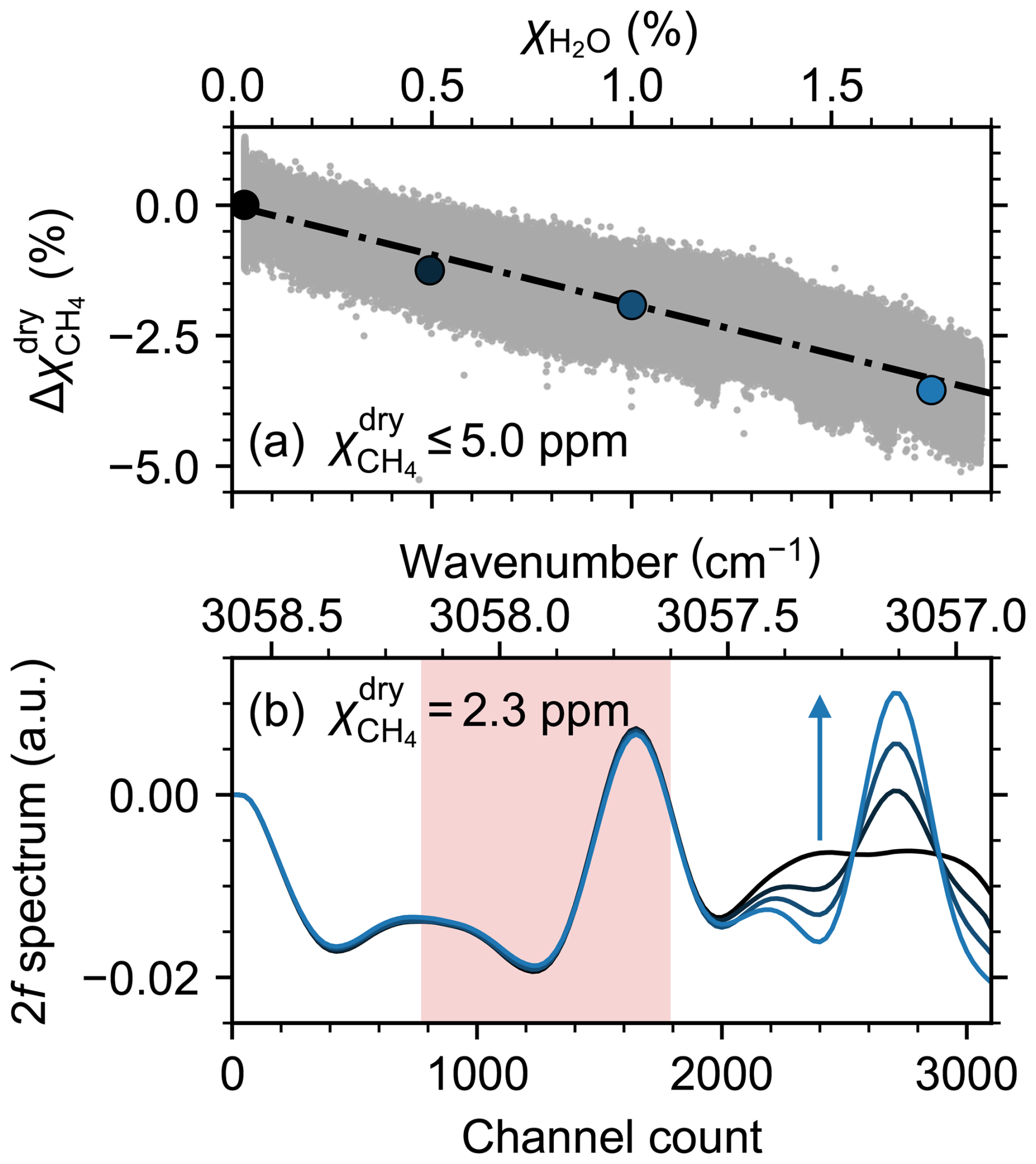
Figure 7 (a) Relative change in the measured methane dry mole fraction as a function of water vapor mole fraction (approximately 0 % to 80 % RH), for methane dry mole fractions below 5 ppm. The dashed black line is a fit to the measured data. (b) 2f spectra for 2.3 ppm methane with water vapor mole fractions 0.03 %, 0.5 %, 1 %, and 1.75 %, corresponding to the large data points in (a). The arrow indicates increasing water vapor content. The shaded region indicates the bounds used to determine the peak-to-peak amplitude for methane.

3.3 Controlled-release experiments

We deployed the ultra-lightweight methane sensor on the DJI Matrice 300 RTK UAV during a controlled-release experiment to evaluate the sensor's capacity to detect methane emissions in the field. To simulate a methane leak, we released methane from a methane gas cylinder (99.5 % purity, AirLiquide, Canada) at a pre-determined flow rate regulated by an MFC. The MFC-regulated methane flow was released through a gas diffuser at the top of a mast. A stationary anemometer was positioned adjacent to the release point to record the wind speed and direction at the source location throughout the experiment.

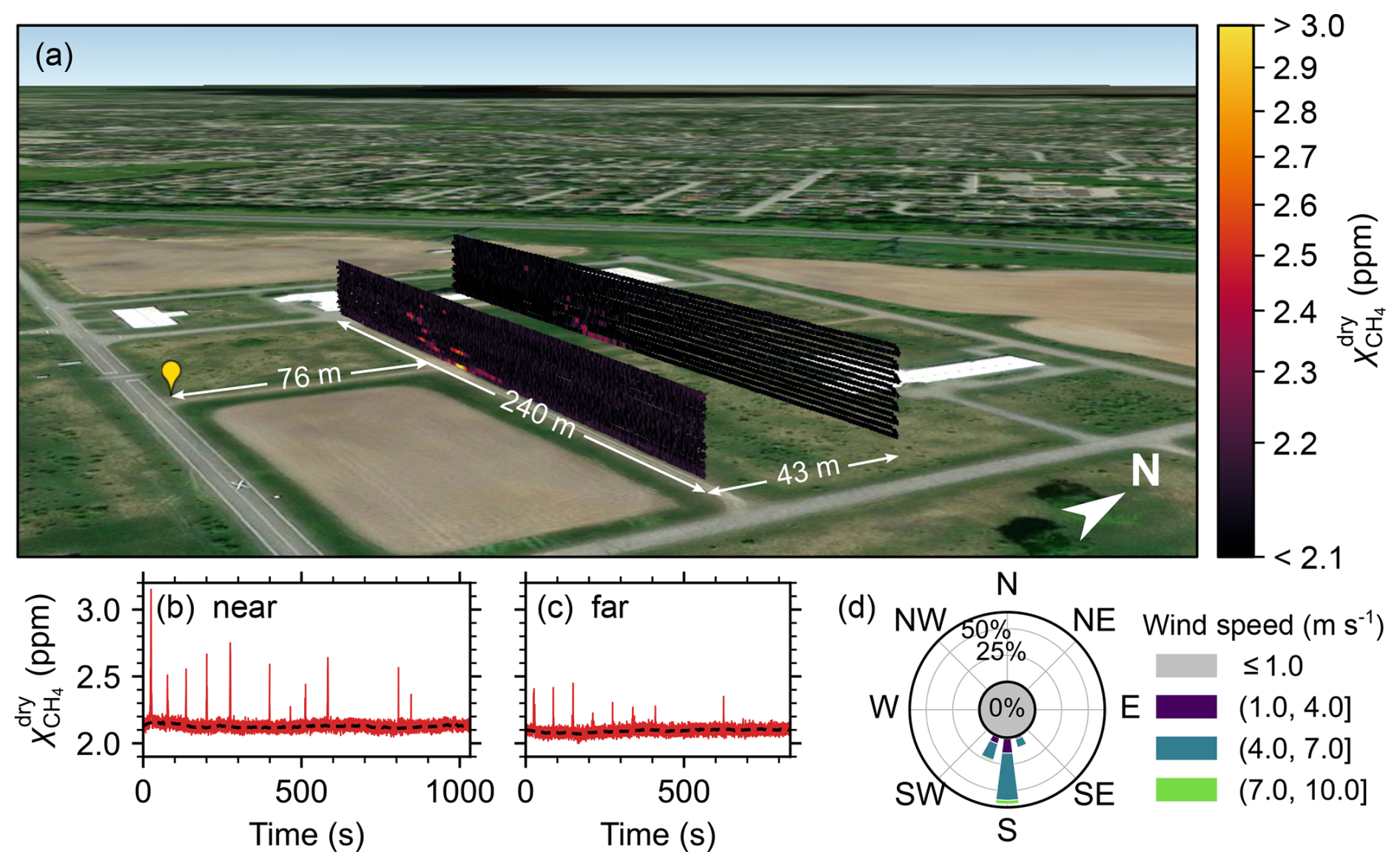
Figure 8 (a) Heat map showing methane dry mole fraction along the UAV flight path for controlled-release experiment. The yellow marker indicates the release point. (b, c) Timeseries datasets corresponding to near and far curtains. The dashed black line indicates the background methane mole fraction. (d) Prevailing wind direction and speed measured at the methane release point. (Maps Data: © Google Earth, Landsat / Copernicus, © 2026 Airbus, © 2026 Vexcel Imaging US, Inc.).

The controlled-release experiment is shown in Fig. 8a. The methane flow rate was 12 standard L min⁻¹ (20 °C and 1013.25 hPa) or 0.48 kg h⁻¹ and the release point was 4.2 m above the ground. To account for adiabatic cooling of the gas upon decompression, we first passed it through a heat exchanger submersed in a thermal bath with an average temperature of 17.5 °C to achieve approximate thermal equilibrium with the ambient temperature. We performed the experiment in a relatively open field on a day when the mean wind speed was 5.3 m s⁻¹ at the release point. The UAV flew two vertical flux curtains at downwind distances of 76 m (near curtain) and 119 m (far curtain) from the emission point. Each horizontal transect spanned a lateral distance of ∼240 m. Transect elevations for the near curtain, which was flown along a dirt road, ranged from 2.5 to 19.5 m above takeoff with transect spacing of 1 m. For the far curtain, uneven terrain and vegetation near the ground prevented the UAV from flying transects below 6.5 m. Transects for the far curtain were spaced at 1.5 m intervals up to a maximum altitude of 26 m above takeoff.

A nearby weather station recorded an average ambient temperature of T=24.2 °C ±1 °C and an average pressure of 1004.6 hPa during the measurement period. The average humidity was 36.7 %, corresponding to an average water vapor mole fraction of 1.1 %.

A uniform +2.1 % correction was applied to the recorded mole fraction data to compensate for relative humidity that differed from dry gas calibration, based on the test results shown in Fig. 7. The temperature during calibration was similar to the average air temperature in the field, therefore temperature correction was not required in this case. After correction, the average value of the background methane dry mole fraction was 2.10±0.10 ppm. The sensor successfully detected enhancements in methane mole fraction above background levels, demonstrating detection at a methane emission rate <0.5 kg h⁻¹, which is below the limit of detection for most conventional aircraft surveys (El Abbadi et al., 2024; Duren et al., 2019; Donahue et al., 2026). Elevated dry mole fractions were detected in the middle of both flux curtains, with the highest values (near: 3.13±0.19 ppm, and far: 2.44±0.15 ppm) observed in the lowest transect. The corresponding timeseries data from the methane sensor is shown in Fig. 8b, c. The flight durations were 17 and 14 min for the near and far curtains, respectively. The prevailing wind speed and direction at the methane release point is shown in Fig. 8d, recorded using a sonic anemometer (WindUltra, Gill Instruments, UK) at a data rate of 2 Hz.

3.3.1 Onboard wind measurements

During the controlled-release experiment, the UAV was equipped with a 2D anemometer for onboard wind measurements. The wind speed and direction recorded by the anemometer at a data rate of 2 Hz were interpolated onto the 10 Hz UAV data stream and corrected using the procedure described in Sect. 2.6. The raw and corrected onboard wind measurements for the near curtain are shown in Fig. 9 along with measurements recorded by the stationary ground anemometer at the release point.

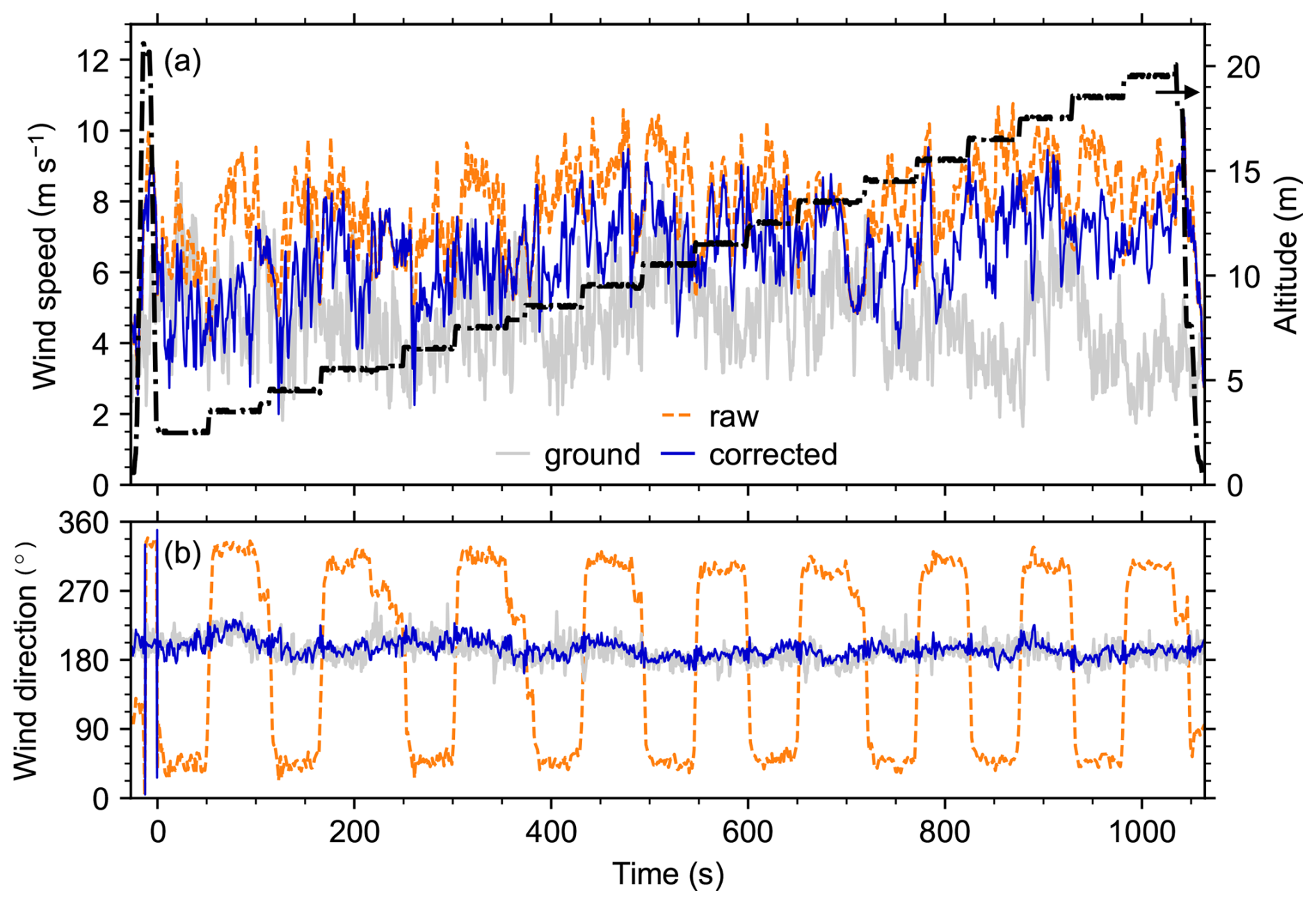
Figure 9 Raw and corrected measurements of (a) wind speed (b) direction recorded by the onboard anemometer for the near curtain. Measurements from the stationary ground anemometer are shown for comparison. UAV height above takeoff is also shown in (a).

After correction, the mean wind direction was 194.3° with a standard deviation of 11.6°. For comparison, the mean wind direction recorded by the stationary anemometer at the release point was 191.3° with a standard deviation of 13.9°. The small discrepancy in the mean direction between the ground and UAV wind measurements is most likely the result of imperfect anemometer north alignment.

As expected, the corrected wind speed increases slightly with altitude. Over the entire flight, the standard deviation in the wind speed is 1.20 m s⁻¹. The standard deviation in the wind speed recorded by the stationary anemometer was 1.26 m s⁻¹. During the flight transect measured at 4.5 m above ground, the average wind speed was 5.48 m s⁻¹, with a standard deviation of 1.13 m s⁻¹. For the same time period, the stationary anemometer, positioned at a height of approximately 4.6 m, recorded an average wind speed of 4.70 m s⁻¹ with a standard deviation of 1.27 m s⁻¹. The difference of 0.7 m s⁻¹ between th e mean values, which is larger than the stated 0.1 m s⁻¹ accuracy of the Gill WindUltra anemometer, is primarily attributed to the spatial separation of the anemometers.

Brief instabilities in the wind speed and direction recorded by the onboard anemometer at takeoff and landing are attributed primarily to interpolation of the 2 Hz wind data, as the data rate was slow compared to the rapid movements of the UAV. We expect that a faster data rate of at least 10 Hz would improve the wind measurement stability during takeoff and landing and improve measurement accuracy by removing the requirement to interpolate. When estimating the uncertainty in the wind speed u, we account for the instrument accuracy, defined as the larger of 2 % or 0.1 m s⁻¹, and the 1σ_u measurement noise. For the wind direction θ, uncertainty includes 1° for instrument accuracy, 5° for anemometer alignment, and the 1σ_θ measurement noise.

3.3.2 Background subtraction

For UAV-based measurements conducted within a few hundred meters of a known point source, the point source does not contribute to the slowly varying background (Morales et al., 2022; Dooley et al., 2024; Shah et al., 2020). Therefore, background methane mole fractions can be found either by flying transects upwind of the known source (Gordon et al., 2015) or using downwind data collected from outside of the plume (Morales et al., 2022). In some cases, where sensor drift or change is known to occur over the course of a measurement, averaging or fitting may be required to accurately define the baseline (Dooley et al., 2024). In this work, we use an averaging approach to extract the baseline from downwind transects. The approach is illustrated in Fig. 10. First, a peak-finding algorithm is used to identify peaks in the recorded methane timeseries data. A mask is defined around each peak such that the signal returns to the baseline on either side. By masking the peaks, we extract the raw background data. A 5.8 s moving average is applied to the background, where the 5.8 s window is chosen because it offers nearly optimal in-flight measurement precision, as determined from the Allan-Werle deviation (see Fig. 4). Linear interpolation is used to estimate the background across each of the peaks, where raw background data is not available. Finally, the elevated methane signal ${\mathit{\chi }}_{{\mathrm{CH}}_{\mathrm{4}}}^{\mathrm{elev}}$ is calculated by subtracting the averaged and interpolated background ${\mathit{\chi }}_{{\mathrm{CH}}_{\mathrm{4}}}^{\mathrm{bkg}}$ from the original measured methane data.

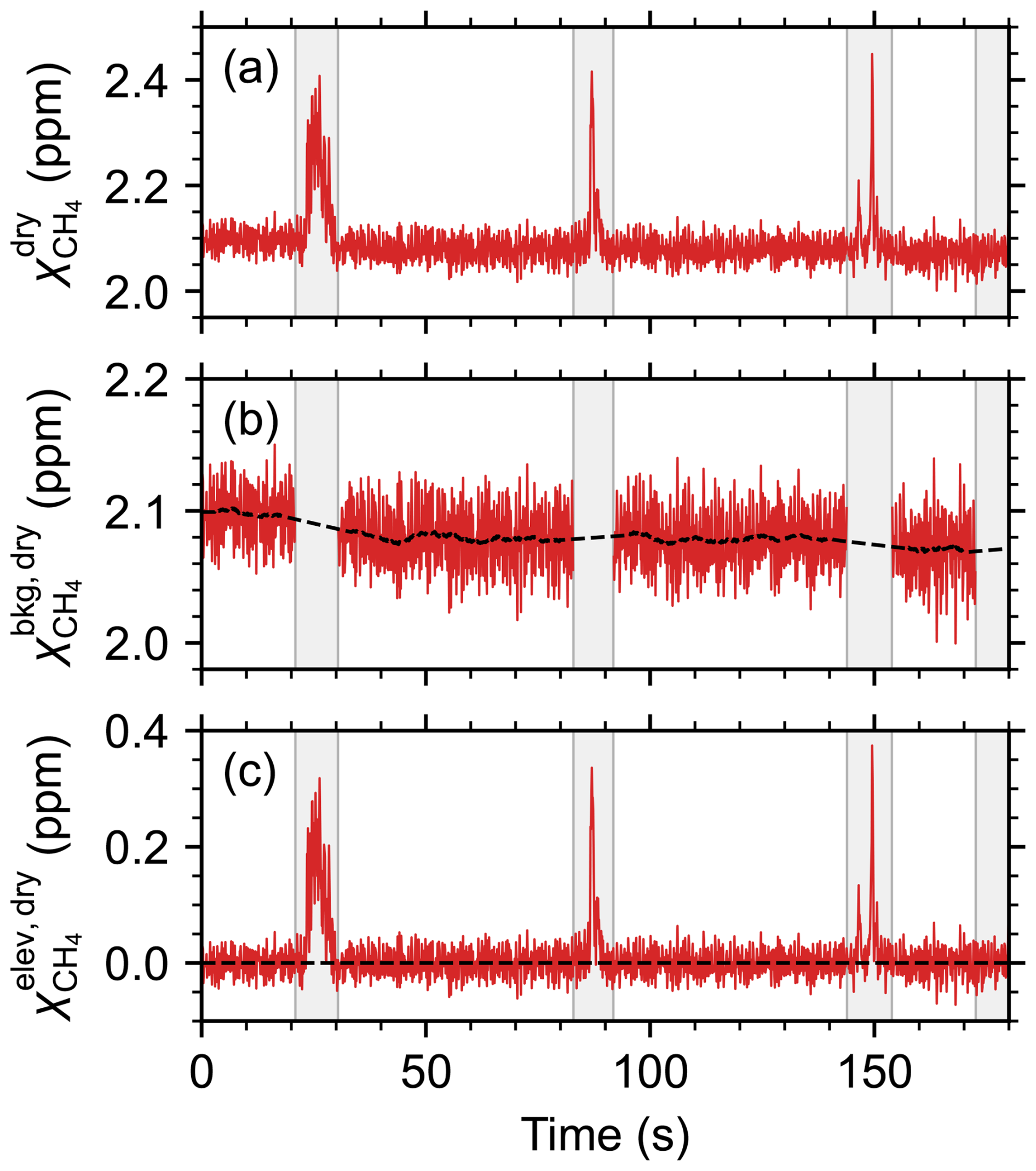
Figure 10 Procedure for extracting the background methane mole fraction, illustrated for the far transect in the controlled-release experiment. (a) Methane dry mole fraction timeseries at 10 Hz. Gray bars represent masks applied to each detected peak. (b) Background methane dry mole fraction with the peaks removed. The black dashed line is the 5.8 s moving average, with linear interpolation over the masked regions. (c) Elevated methane dry mole fraction.

To confirm that no unidentified point sources were contributing to the observed methane enhancements, several transects were flown directly upwind of the release location. The timeseries data from the upwind flight showed no evidence of additional point sources.

3.3.3 In-flight stability and performance

As discussed in Sect. 3.2, the open-path methane sensor is sensitive to changing environmental conditions. To asses the instrument's stability and performance when deployed on a UAV, we compare the timeseries datasets from the controlled-release for a collection of instrument, environmental, and flight parameters, shown in Fig. 11. We have included 60 s of data immediately before takeoff and after landing. The gray shaded regions at the beginning and end of each timeseries indicate data that falls outside of the defined flux curtain flightpath–this data is discarded when calculating the emission flux. The methane mole fraction, shown at the top, is scaled to emphasize the slowly varying background. Over the segments of data that are used for flux quantification, ${\mathit{\chi }}_{{\mathrm{CH}}_{\mathrm{4}}}^{\mathrm{bkg},\mathrm{dry}}$, indicated by the black dashed line in the top panels of Fig. 11, has a maximum drift of 2.5 % for the near curtain and 2.1 % for the far curtain. More significant drift, up to 5 % (∼100 ppb), is observed outside of the flux curtains, notably during takeoff and landing, however these effects appear to be self-limiting as the signal stabilizes quickly. The 2f peak and trough channel positions are generally stable and remain well within the search bounds defined in Fig. 2, indicating that spectral drift over the measurement period is minimal. Drift is known to affect other UAV-borne sensors including commercial instruments such as the Aeris MIRA Pico and Strato sensors (Dooley et al., 2024; Bolek et al., 2026). Notably, Dooley et al. (2024) showed a systematic drift of roughly 250 ppb over a 20 min UAV flight for a MIRA Pico sensor.

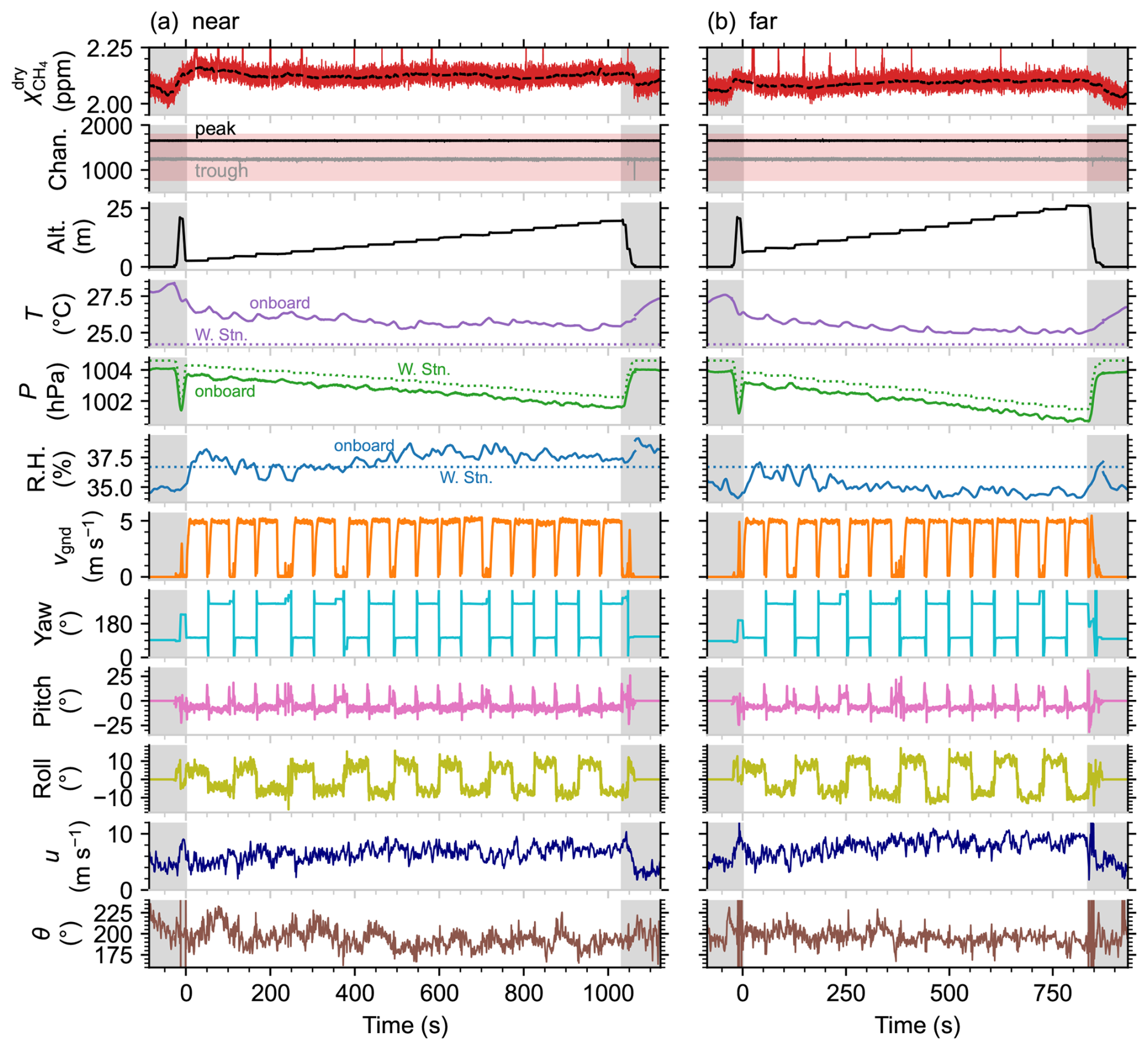
Figure 11 Collection of parameters recorded over time for controlled-release (a) near and (b) far curtain flights. In order from top to bottom, the parameters are: methane dry mole fraction, 2f peak and trough channel numbers (Chan.), altitude (Alt.), temperature (T), pressure (P), relative humidity (RH), ground speed (v_gnd), heading (yaw), pitch, roll, wind speed (u), and wind direction (θ). The gray shaded bars at the beginning and end of each timeseries indicate data that falls outside of the defined flux curtain, including UAV takeoff and landing. The methane mole fraction scale is adjusted to emphasize the slowly varying baseline, displaying both the 10 Hz time series and the 5.8 s moving average of the background (black dashed line). The red shaded region in the peak and trough channel plot indicates the search bounds defined in Fig. 2. T, P, and RH measurements are shown for both the onboard sensor (10 s moving average) and average values from a local weather station (W. Stn.). Wind speed and direction were from the onboard anemometer.

Temperature, pressure, and relative humidity were continuously measured throughout each flight using the onboard BME280 sensor, which was affixed to the methane sensor baseplate. For comparison, data from a nearby local weather station are also shown in Fig. 11. Because only hourly data was available from the weather station, its data were linearly interpolated over the entire flight period and averaged. The station pressure was corrected to account for the altitude difference between the station and the UAV throughout each flight. Analysis of the in-flight timeseries reveals significant temperature fluctuations recorded by the onboard sensor that appear to be correlated with rapid changes in the UAV ground speed (v_gnd). Similar variability is also observed in the onboard relative humidity data. These observations are consistent with laboratory measurements, which have indicated that the onboard BME280 sensor is influenced by changes in airflow. Furthermore, the onboard sensor reports higher temperatures than the local weather station. This is consistent with laboratory observations showing that the onboard sensor typically reports temperatures several degrees higher than those measured by independent sensors, likely because the sensor baseplate is warmer than surrounding air during operation. Given these limitations, average temperature and relative humidity values from the weather station were used in the emission flux calculations described in Sect. 3.3.4. Nonetheless, the onboard measurements offer a rough sense of how temperature may have varied during the flight, even though the absolute values and rapid variations are not considered reliable. Despite the challenges with onboard temperature and relative humidity, onboard pressure measurements show good agreement with the expected values derived from the weather station data, deviating by a maximum of 1 hPa.

When comparing variations in the background methane mole fraction to the other timeseries datasets shown in Fig. 11, no apparent correlations are observed. Though other airborne spectroscopic gas analyzers have been shown to be strongly influenced by rapid changes in the movement of the aircraft (Ort et al., 2024), the open-path instrument does not appear to be affected by rapid in-flight variations in the UAV ground speed, yaw, pitch, or roll. Likewise, change in wind speed and direction do not appear to influence the instrument response. The observed drift is therefore attributed primarily to changes in temperature, pressure, relative humidity, and air flow (during takeoff and landing), which are known to affect the recorded mole fractions. More accurate and comprehensive onboard measurements of environmental conditions are needed to discern and mitigate the effects that impact the sensor's reading.

The in-flight measurements are used in tandem with results from laboratory experiments to estimate uncertainty on the methane mole fraction. The statistical component of the methane calibration error is set to 3 %. This is a conservative estimate that accounts for the 1σ calibration uncertainty (<1.5 %) and in-flight measurement drift (<2.5 %) added in quadrature. Measurement precision is also considered in the statistical error analysis, contributing 27 ppb for a 0.1 s averaging time and 3.5 ppb for the optimal 5.8 s averaging time used when analyzing the slowly varying background signal. Additionally, though the measured data was corrected to compensate for the difference in relative humidity compared to calibration, uncertainty in the correction factor and in the environmental conditions remains. For this reason, we apply a conservative systematic uncertainty of 5 % in addition to the statistical uncertainty. This 5 % is intended to account for variability in the signal strength observed with changing temperature and humidity, as discussed in Sect. 3.2, as well as potential pressure-related effects.

3.3.4 Emission flux quantification

The emission flux rate was estimated from the curtain flights conducted during the controlled-release experiment, using the procedure described in Sect. 2.7. Figure 12a and b show heat maps of the measured flux density q for the far and near flux curtains, calculated per Eq. (5) from the elevated methane mole fraction, the orthogonal wind field (measured by the anemometer mounted on the UAV), the average temperature (recorded by the weather station), and the on-board pressure data, which varied with altitude according to the relation $P\left(z\right)=-\mathrm{0.121}z+\mathrm{1003.9}$ hPa.

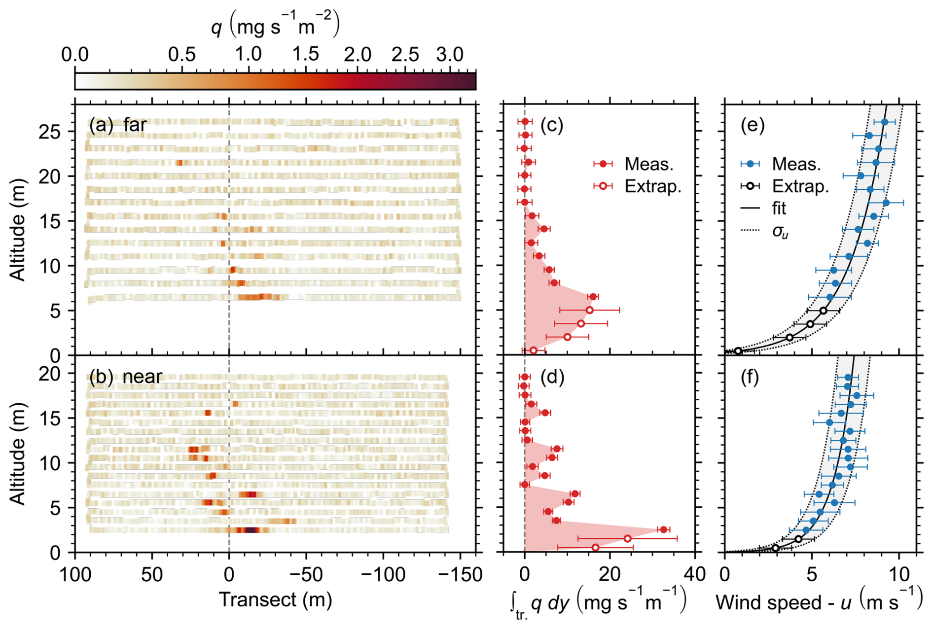
Figure 12 (a, b) Heat maps showing methane flux density along the UAV flight path for the far and near curtains. (c, d) Corresponding transect-integrated flux density for each horizontal transect. The shaded regions correspond to the estimated total emission flux and error bars indicate 1σ uncertainties. (e, f) Average wind speed and standard deviation along each horizontal transect and fit to logarithmic wind model including 1σ_u prediction interval. Extrapolated transects are indicated by the open markers.

The corresponding transect-integrated flux densities, ${\int }_{\mathrm{tr}.}q\mathrm{d}y$, are shown in Fig. 12c and d, with error bars indicating the propagated 1σ uncertainties attributed to random (statistical) error in the calibration, in-flight precision, and the standard deviation in the measured wind speed and direction. Estimated statistical and systematic uncertainties are summarized in Table A2. The position of the DJI Matrice 300 RTK UAV is recorded to a precision of 1 cm in the horizontal direction and 1.5 cm in the vertical direction. These small uncertainties are treated as negligible given that the flux planes span tens of meters vertically and hundreds of meters horizontally.

A constant transect-integrated methane mole fraction was defined from the lowest transect to the ground, where ${\int }_{\mathrm{tr}.}{\mathit{\chi }}_{{\mathrm{CH}}_{\mathrm{4}}}\mathrm{d}y=\mathrm{4.1}\pm \mathrm{1.8}\mathrm{ppm}\mathrm{m}$ for the far curtain and 8.8±3.8 ppm m for the near curtain. Fitting the logarithmic wind model (Eq. 7) to the wind data recorded from the UAV, friction velocity and surface roughness parameters $u^{*}=\mathrm{0.842}\pm \mathrm{0.024}$ m s⁻¹ and $z_{\mathrm{0}}=\mathrm{0.340}\pm \mathrm{0.029}$ m, respectively, were obtained for the far flux curtain. For the near curtain, the parameters were found to be $u^{*}=\mathrm{0.475}\pm \mathrm{0.014}$ m s⁻¹ and $z_{\mathrm{0}}=\mathrm{0.042}\pm \mathrm{0.005}$ m. The differences in the logarithmic wind fields are attributed to the rougher terrain beneath the far flux curtain and to changing wind conditions over time, as the total experiment took 54 min, including a 23 min logistical delay between completing the near curtain and beginning to fly the far curtain.

The shaded regions in Fig. 12c, d correspond to the estimates for total methane emission flux, $Q=\mathrm{0.44}\pm \mathrm{0.18}$ kg h⁻¹ and $Q=\mathrm{0.47}\pm \mathrm{0.22}$ kg h⁻¹ for the far and near flux curtains, respectively. The reported 2σ error bounds correspond to relative uncertainties of 40 % (far) and 47 % (near). The true methane release rate, 0.48 kg h⁻¹, falls well within uncertainty for both estimated flux rates, differing by 8.7 % for the far curtain and 1.1 % for the near. For comparison, Bonne et al. (2024) applied a similar quantification method and demonstrated a prediction error ranging from −69 % to 150 % over 45 flights, and from −50 % to 100 % for 80 % of the flights, relative to the actual release rate. Scheutz et al. (2025) published results from 12 controlled release flights and demonstrated predictions with a relative error in the range of −35.4 % to 33.4 % compared to the true rate.

A detailed explanation of the error propagation, including estimated uncertainties for vertical extrapolation and interpolation, can be found in the Appendix. Relative 1σ uncertainty contributions are listed by error source in Table A2. The largest sources of error in the estimated flux rate are the interpolation between horizontal transects and the extrapolation between the lowest measured transect and the ground. Furthermore, if the lowest measured transect is neglected from the flux calculation and extrapolation is carried out from the next-lowest transect, the computed flux rates would be $Q=\mathrm{0.26}\pm \mathrm{0.10}$ kg h⁻¹ (far) and $Q=\mathrm{0.30}\pm \mathrm{0.12}$ kg h⁻¹ (near), far from the true release rate. This underscores the importance of flying transects as close to the ground as possible when mapping low-lying plumes in the near-field.

Though we aimed to include as many sources of error as possible in the uncertainty estimation, one uncertainty element that is not fully accounted for is due to atmospheric turbulence and the non-stationary nature of the measured plume. When considering a single curtain flight recorded over a period of approximately 15 min, atmospheric turbulence causes variation between the horizontal transects that is not reflected in the mass-balance flux estimation. The associated uncertainty contribution is therefore partially accounted for in the interpolation and extrapolation error estimates, which evaluate the impact of individual transects on the estimated emission flux (see Appendix A). However, a statistical analysis over many curtain flights would be required for rigorous accounting of the atmospheric turbulence effect, which is beyond the scope of this demonstration. A detailed discussion of how turbulent atmospheric conditions affect emission flux estimation can be found in Conley et al. (2017).

4 Summary and conclusions

In this work, we developed a compact, ultra-lightweight methane sensor platform for in-situ measurements and deployed it on a small enterprise-grade UAV in a controlled-release experiment to evaluate its potential to quantify fugitive methane emissions. The sensor is based on tunable diode laser absorption spectroscopy and targets methane gas in the mid-IR using a HgCdTe photodetector and a GaSb-based DFB laser centered at 3270.4 nm. The instrument employs an open-path multi-pass absorption cell for fast response times (up to 100 Hz) and wavelength modulation spectroscopy for improved signal-to-noise. A small single board computer and custom data acquisition PCB facilitated the miniaturization of a complete data acquisition and control system with real-time onboard WMS data processing and local data storage capabilities. Compared with its predecessor, the new instrument is 84 % smaller, 75 % lighter, and consumes 40 % less power. Where possible, commercially available off-the-shelf components were used in the sensor design to facilitate the adoption and widespread use of this measurement technique. A lower-cost system could be achieved using silver or aluminum mirrors in place of gold and by replacing the mid-IR light source and photodetector with near-IR alternatives for applications where the enhanced resolution provided by mid-IR sources is not required. Although our research demonstrates the sensor’s application for methane, the same platform could be adapted to other gaseous species by substituting the laser and photodetector to target absorption features specific to the molecule of interest. Differences in atmospheric abundance or absorption cross section may require further optomechanical or electronics adaptations; however, the core design principles remain broadly transferable.

Weighing just 1.2 kg, including the dedicated battery, this is one of the lightest spectroscopic methane gas sensors reported to date. It is also extremely power efficient, consuming approximately 11 W of electrical power when the ambient temperature is around 20 °C, enabling continuous operation for more than 2 h. When the sensor is installed together with the anemometer assembly on a DJI Matrice 300 RTK UAV, several consecutive flights of approximately 20 min each can be carried out sequentially without needing to power off the sensor.

The sensor achieves an in-flight precision of 6.7 ppb at 1 Hz which, to our knowledge, is the best 1 Hz precision for a UAV-borne methane sensor weighing less than 2 kg reported to date. The in-flight precision could be further improved by mitigating inductive noise produced by the sensor's on-board radio, used for real-time data streaming. Laboratory measurements without real-time data streaming show a 1 Hz precision of 3.7 ppb. When deployed on a fast-moving UAV platform traveling at 5–8 m s⁻¹, a 10 Hz time resolution is used for signal averaging, corresponding to an in-flight measurement precision of 27 ppb. In-flight drifts of up to 100 ppb were observed in the background methane signal over the course of a 20 min flight, with the largest drifts seen at takeoff and landing. Drifts are attributed primarily to changes in ambient conditions and airflow. Laboratory experiments revealed a non-linear dependence on ambient air temperature and a linear dependence on water vapor mole fraction. Detailed characterization of these effects and improved on-board temperature and relative humidity measurements could facilitate the implementation of robust on-line corrections, which would enable more accurate quantification of background methane levels. However, sensor drift is not expected to be a dominant source of error when quantifying emissions from a near-by point source.

The system was deployed in a controlled-release experiment with a methane release rate of 0.48 kg h⁻¹, below the detection limit for most conventional aircraft methane sensing systems. Using a direct mass balance flux quantification approach, the true emission rate was obtained to within 9 % under steady winds and at downwind distances of <120 m from the release point. In this demonstration for which the methane source was positioned just a few meters above the ground, the accuracy of the retrieved emission rate was found to depend heavily on the lowest measured transects, which contained the highest methane content. To fully evaluate this UAV-based emission rate quantification approach, further systematic and statistical studies are needed to assess how variables such as meteorological conditions, source parameters, flight patterns, and terrain topography influence the probability of detection and quantification accuracy.

Overall, we have developed a high-precision ultra-lightweight gas sensor optimized for deployment on small UAVs. We have demonstrated that this is a promising method for targeted detection and quantification of emission sources near the ground and over terrain that is inaccessible to or cannot be measured by alternative measurement platforms. The platform is well suited for characterizing anthropogenic emissions from sources such as oil and gas facilities (well sites, compressor stations, gas processing plants), wastewater treatment facilities, and small landfills, and has also been used to quantify emissions from naturally occurring geologic gas seeps (Bolek et al., 2026). We have demonstrated promising detection and quantification capability at emission rates near 0.5 kg h⁻¹ and expect that even smaller sources could be characterized using this instrument by mitigating inductive noise or adapting flight strategies to accommodate longer averaging times, which would enhance the measurement precision. These results highlight the ultra-lightweight methane sensor's potential as a flexible and scalable solution for monitoring methane emissions across a wide range of environments.

Appendix A: Uncertainty analysis for emission flux quantification

This section describes the procedure used to propagate uncertainty in the emission flux quantification. The uncertainties assigned to parameters used in the calculation of methane flux density (q) are summarized in Table A1.

Table A1 Estimated uncertainty on parameters used in flux quantification.

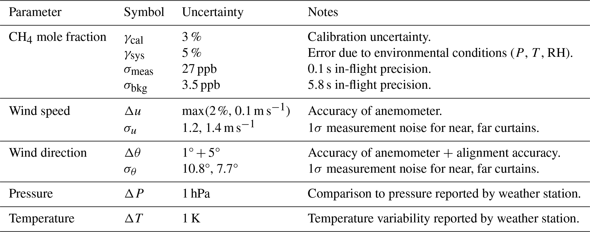
Uncertainty on the methane mole fraction is broken down into several components. The calibration uncertainty γ_cal accounts for both error and drift in the instrument calibration. The value of 3 % is a conservative estimate that accounts for the 1σ calibration uncertainty and residuals for the calibration performed immediately prior to the controlled-release experiment. γ_cal is treated as a random error component. The instrument precision is also included in the analysis as random error. We assign a systematic error component γ_sys, which accounts for error introduced by variations in temperature, pressure, and relative humidity. Systematic error is treated separately from random error.

The elevated methane mole fraction is given by ${\mathit{\chi }}_{{\mathrm{CH}}_{\mathrm{4}}}^{\mathrm{elev}}={\mathit{\chi }}_{{\mathrm{CH}}_{\mathrm{4}}}^{\mathrm{meas}}-{\mathit{\chi }}_{{\mathrm{CH}}_{\mathrm{4}}}^{\mathrm{bkg}}$, where ${\mathit{\chi }}_{{\mathrm{CH}}_{\mathrm{4}}}^{\mathrm{bkg}}$ is computed by removing the peaks from ${\mathit{\chi }}_{{\mathrm{CH}}_{\mathrm{4}}}^{\mathrm{meas}}$ and applying a 60 s rolling average. The calibration uncertainties for ${\mathit{\chi }}_{{\mathrm{CH}}_{\mathrm{4}}}^{\mathrm{meas}}$ and ${\mathit{\chi }}_{{\mathrm{CH}}_{\mathrm{4}}}^{\mathrm{bkg}}$ are highly correlated because they share the same calibration and are measured in close spatial and temporal proximity. Conversely, the uncertainty contributions derived from the measurement precision (σ_meas and σ_bkg) are not correlated. The estimated random error on the elevated methane mole fraction is therefore:

$$\begin{array}{}\text{(A1)}& \mathit{\delta }{\mathit{\chi }}_{{\mathrm{CH}}_{\mathrm{4}}}^{\mathrm{elev}}=\sqrt{{\left({\mathit{\gamma }}_{\mathrm{cal}}{\mathit{\chi }}_{{\mathrm{CH}}_{\mathrm{4}}}^{\mathrm{meas}}-{\mathit{\gamma }}_{\mathrm{cal}}{\mathit{\chi }}_{{\mathrm{CH}}_{\mathrm{4}}}^{\mathrm{bkg}}\right)}^{\mathrm{2}}+{\mathit{\sigma }}_{\mathrm{meas}}^{\mathrm{2}}+{\mathit{\sigma }}_{\mathrm{bkg}}^{\mathrm{2}}}\end{array}$$

The orthogonal wind speed is given by u_x=ucos (θ). The random error on u_x=ucos (θ) is therefore:

$$\begin{array}{}\text{(A2)}& \mathit{\delta }{u}_x=\sqrt{(\cos \mathit{\theta }{\mathit{\sigma }}_u{)}^{\mathrm{2}}+(u\sin \mathit{\theta }{\mathit{\sigma }}_{\mathit{\theta }}{)}^{\mathrm{2}}}\end{array}$$

The methane flux density is given by $q={\mathit{\chi }}_{{\mathrm{CH}}_{\mathrm{4}}}^{\mathrm{elev}}{u}_x\mathit{\rho }$, and so its propagated uncertainty due to random error contributions is:

$$\begin{array}{}\text{(A3)}& \mathit{\delta }q=q\sqrt{{\left({\displaystyle \frac{\mathit{\delta }{\mathit{\chi }}_{{\mathrm{CH}}_{\mathrm{4}}}^{\mathrm{elev}}}{{\mathit{\chi }}_{{\mathrm{CH}}_{\mathrm{4}}}^{\mathrm{elev}}}}\right)}^{\mathrm{2}}+{\left({\displaystyle \frac{\mathit{\delta }{u}_x}{u_x}}\right)}^{\mathrm{2}}}\end{array}$$

The transect-integrated flux density is computed numerically using the trapezoid rule:

$$\begin{array}{}\text{(A4)}& f_{\mathrm{tr}.}\left(z\right)=\underset{\mathrm{tr}.}{\int }q(y,z)\mathrm{d}y=\sum _{i=\mathrm{0}}^{n-\mathrm{2}}{\displaystyle \frac{(q_i+q_{i+\mathrm{1}})}{\mathrm{2}}}(y_{i+\mathrm{1}}-y_i)\end{array}$$

where y is the horizontal position of the UAV and n is the number of elements in the transect. The random uncertainty in ${\int }_{\mathrm{tr}.}q\mathrm{d}y$ is then:

$$\begin{array}{}\text{(A5)}& \begin{array}{rl}& \mathit{\delta }{f}_{\mathrm{tr}.}\left(z\right)=\sqrt{\sum _{i=\mathrm{0}}^{n-\mathrm{2}}(\mathit{\delta }{q}_i{w}_i{)}^{\mathrm{2}}},\\ & w_i=\left\{\begin{array}{ll}\frac{\mathrm{1}}{\mathrm{2}}(y_{\mathrm{1}}-y_{\mathrm{0}}),& i=\mathrm{0}\\ \frac{\mathrm{1}}{\mathrm{2}}(y_{i+\mathrm{1}}-y_{i-\mathrm{1}}),& \mathrm{0}<i<n-\mathrm{2}\\ \frac{\mathrm{1}}{\mathrm{2}}(y_{n-\mathrm{1}}-y_{n-\mathrm{2}}),& i=n-\mathrm{2}\end{array}\right.\end{array}\end{array}$$

Due to the close spatial and temporal proximity of the data points along each transect, we assume that the uncertainty contribution of the linear interpolation along horizontal transects is negligible.

The estimated transect-integrated flux density for the extrapolated transects (tr. exp.) between the lowest measured transect and the ground (z=0) is given by:

$$\begin{array}{}\text{(A6)}& f_{\mathrm{tr}.\mathrm{ext}.}\left(z\right)=\underset{\mathrm{tr}.\mathrm{ext}.}{\int }q(y,z)\mathrm{d}y=\stackrel{\mathrm{‾}}{{\mathit{\chi }}_{{\mathrm{CH}}_{\mathrm{4}}}^{\mathrm{ext}.}}{u}_{\mathrm{ext}.}\left(z\right)\mathit{\rho }\left(z\right)\end{array}$$

where $\stackrel{\mathrm{‾}}{{\mathit{\chi }}_{{\mathrm{CH}}_{\mathrm{4}}}^{\mathrm{ext}.}}={\int }_{\mathrm{tr}.\mathrm{low}.}{\mathit{\chi }}_{{\mathrm{CH}}_{\mathrm{4}}}^{\mathrm{elev}}\mathrm{d}y$ is the transect-integrated methane mole fraction for the lowest measured transect, computed using the trapezoid rule, and u_ext.(z) is the extrapolated wind speed obtained from the logarithmic wind model (Eq. 7). The estimated uncertainty on $f_{\mathrm{tr}.\mathrm{ext}.}\left(z\right)$ is given by:

$$\begin{array}{}\text{(A7)}& \mathit{\delta }{f}_{\mathrm{tr}.\mathrm{ext}.}=f_{\mathrm{tr}.\mathrm{ext}.}\sqrt{{\left({\displaystyle \frac{\mathrm{0.43}\stackrel{\mathrm{‾}}{{\mathit{\chi }}_{{\mathrm{CH}}_{\mathrm{4}}}^{\mathrm{ext}.}}}{\stackrel{\mathrm{‾}}{{\mathit{\chi }}_{{\mathrm{CH}}_{\mathrm{4}}}^{\mathrm{ext}.}}}}\right)}^{\mathrm{2}}+{\left({\displaystyle \frac{\mathit{\delta }{u}_{\mathrm{ext}.}}{u_{\mathrm{ext}.}}}\right)}^{\mathrm{2}}}\end{array}$$

$\mathrm{0.43}\stackrel{\mathrm{‾}}{{\mathit{\chi }}_{{\mathrm{CH}}_{\mathrm{4}}}^{\mathrm{ext}.}}$ is the standard deviation for a normal distribution centered at $\stackrel{\mathrm{‾}}{{\mathit{\chi }}_{{\mathrm{CH}}_{\mathrm{4}}}^{\mathrm{ext}.}}$ for which the probability that the transect-integrated methane mole fraction $\stackrel{\mathrm{‾}}{{\mathit{\chi }}_{{\mathrm{CH}}_{\mathrm{4}}}}>\mathrm{0}\mathrm{ppm}\cdot \mathrm{m}$ is 99 %. This is to say that the transect-integrated methane mole fraction for the extrapolated transect is likely similar to $\stackrel{\mathrm{‾}}{{\mathit{\chi }}_{{\mathrm{CH}}_{\mathrm{4}}}^{\mathrm{ext}.}}$, and unlikely to be zero–a plausible assumption for a methane source located just a few meters above the ground. δu_ext. corresponds to the 1σ prediction interval from the logarithmic wind model.

The total estimated flux is found by integrating over the transect-integrated flux densities between z=0 and the top measurement transect using the trapezoid rule:

$$\begin{array}{}\text{(A8)}& Q=\underset{\mathrm{0}}{\overset{z_{\max }}{\int }}{f}_{\mathrm{tr}.}\left(z\right)\mathrm{d}z=\sum _{i=\mathrm{0}}^{m-\mathrm{2}}{\displaystyle \frac{\left(f_{\mathrm{tr}.,i}+f_{\mathrm{tr}.,i+\mathrm{1}}\right)}{\mathrm{2}}}\left(z_{i+\mathrm{1}}-z_i\right)\end{array}$$

where m is the number of transects (both measured and extrapolated). The uncertainty on Q due to the statistical components δf_tr. and the extrapolation uncertainties $\mathit{\delta }{f}_{\mathrm{tr}.\mathrm{ext}.}$ is given by:

$$\begin{array}{}\text{(A9)}& \begin{array}{rl}& \sqrt{\mathit{\delta }{Q}_{\mathrm{stat}.}^{\mathrm{2}}+\mathit{\delta }{Q}_{\mathrm{extrap}.}^{\mathrm{2}}}=\sqrt{\sum _{i=\mathrm{0}}^{m-\mathrm{2}}(\mathit{\delta }{f}_{\mathrm{tr}.,i}{h}_i{)}^{\mathrm{2}}},\\ & h_i=\left\{\begin{array}{ll}\frac{\mathrm{1}}{\mathrm{2}}(z_{\mathrm{1}}-z_{\mathrm{0}}),& i=\mathrm{0}\\ \frac{\mathrm{1}}{\mathrm{2}}(z_{i+\mathrm{1}}-z_{i-\mathrm{1}}),& \mathrm{0}<i<m-\mathrm{2}\\ \frac{\mathrm{1}}{\mathrm{2}}\left(z_{m-\mathrm{1}}-z_{m-\mathrm{2}}\right),& i=m-\mathrm{2}\end{array}\right.\end{array}\end{array}$$

Table A2 Summary of relative 1σ error contributions for controlled-release experiment flux estimates. Statistical (stat.) and systemic (syst.) error sources are indicated.

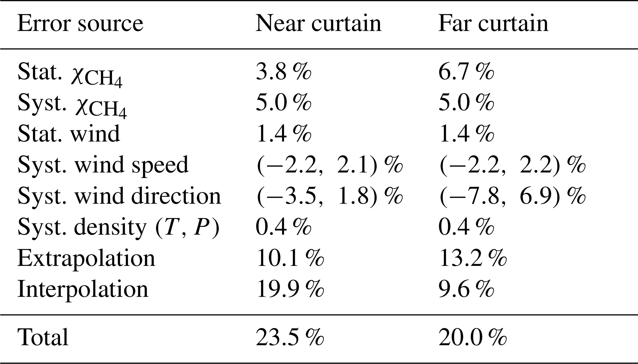
The spatial and temporal separation of the transects results in a significant uncertainty when interpolating in z. We estimate the uncertainty in the linear interpolation by implementing a leave one out cross validation protocol. For each $f_{\mathrm{tr}.,i}$ from i=1 to m−2, we remove the transect and predict its value by interpolating linearly between $f_{\mathrm{tr}.,i-\mathrm{1}}$ and $f_{\mathrm{tr}.,i+\mathrm{1}}$. We then use the residuals to estimate the root mean square error:

$$\begin{array}{}\text{(A10)}& \mathit{\delta }{f}_{\mathrm{interp}.}=\sqrt{\frac{\mathrm{1}}{m-\mathrm{2}}\sum _{i=\mathrm{1}}^{m-\mathrm{2}}(f_{\mathrm{tr}.,i}-f_{\mathrm{pred}.,i}{)}^{\mathrm{2}}}\end{array}$$

The estimated interpolation error for each transect is then propagated to compute the cumulative interpolation uncertainty:

$$\begin{array}{}\text{(A11)}& \begin{array}{rl}& \mathit{\delta }{Q}_{\mathrm{interp}.}=\sqrt{\sum _{i=\mathrm{0}}^{m-\mathrm{2}}(\mathit{\delta }{f}_{\mathrm{interp}.}{h}_i{)}^{\mathrm{2}}},\\ & h_i=\left\{\begin{array}{ll}\frac{\mathrm{1}}{\mathrm{2}}(z_{\mathrm{1}}-z_{\mathrm{0}}),& i=\mathrm{0}\\ \frac{\mathrm{1}}{\mathrm{2}}(z_{i+\mathrm{1}}-z_{i-\mathrm{1}}),& \mathrm{0}<i<m-\mathrm{2}\\ \frac{\mathrm{1}}{\mathrm{2}}(z_{m-\mathrm{1}}-z_{m-\mathrm{2}}),& i=m-\mathrm{2}\end{array}\right.\end{array}\end{array}$$

The remaining uncertainty contributions come from systematic errors in the methane mole fraction, wind speed and direction, and methane density (computed from temperature and pressure). The relevant contributions are summarized in Table A1. These uncertainties are treated by calculating the emission flux Q at the upper and lower bounds for each parameter. The total uncertainty on Q is calculated using the dimidiated Gaussian model to propagate asymmetric errors (Barlow et al., 2026). The relative error contributions for the two curtain flights are summarized in Table A2.