A self-supervised and distillation-guided framework for robust cloud-layer identification in multi-channel Raman lidar networks

Cloud-layer identification is a key prerequisite for automated ground-based lidar processing, but remains challenging in Raman lidar networks because of incomplete near-range overlap, weak high-level cloud echoes, day-night signal-to-noise ratio (SNR) contrasts, energy fluctuations, and aerosol-cloud ambiguity. Leveraging the China Aerosol Raman Lidar Network (CARLNET), we propose a multi-channel cloud-layer identification framework that operates on 355/532/1064 nm elastic signals and 355/532 nm volume depolarization ratios, reducing dependence on absolute calibration and retrieved optical products. The framework combines an anisotropic encoder-decoder architecture with a three-stage training strategy, including self-supervised pretraining, traditional-algorithm-guided probabilistic distillation, and fine-tuning with limited expert refinement. Strict cross-site and cross-time evaluation on held-out sites shows that, without using any test-site observations during pretraining or test-site annotations during fine-tuning, the framework achieves an F1 score of 0.937. Compared with direct supervised training, the pretrained model yields comparable cloud-base accuracy (MAE: 59.1 versus 55.3 m) while reducing the detectable cloud-top MAE from 94.0 to 82.2 m. It also substantially outperforms the conventional VDE baseline in both cloud-base and cloud-top estimation. Independent evaluation based on a total of 47 matched lidar–radiosonde cases aggregated across the three held-out sites yields a structural consistency rate of 38.3 % with radiosonde-derived moist layers, compared with 34.0 % for VDE, providing an independent structural-consistency assessment across the two observing systems. These results demonstrate a cloud-layer identification technique that is transferable across held-out CARLNET sites and reduces dependence on absolute calibration, supporting network-scale Raman lidar processing.

1 Introduction

Ground-based lidar systems provide vertically resolved observations of atmospheric aerosols and clouds with high spatial resolution and continuous temporal sampling, making them important instruments for automated atmospheric profiling and long-term network observations (Campbell et al., 2002; Illingworth et al., 2007; Baars et al., 2016; Yin et al., 2020; He et al., 2024; Jing et al., 2025). Multi-wavelength Raman-polarization lidars further provide complementary information from elastic backscatter, Raman signals, and depolarization measurements, which can support aerosol-cloud discrimination, optical retrieval, and cloud-structure characterization (Sassen, 1991; Zhao et al., 2012; Thorsen et al., 2015; Alizadeh-Choobari and Gharaylou, 2017; Baars et al., 2017). However, the information content of lidar observations is strongly height-dependent. In the near range, incomplete overlap and the instrument blind zone can make low-level clouds and cloud bases difficult to detect reliably. At higher altitudes, weak backscatter signals, solar background, and increasing molecular-noise contributions make optically thin clouds, especially high-level cirrus, vulnerable to missed detections and uncertain boundary placement. These characteristics make robust cloud-layer identification a necessary but non-trivial step in automated lidar processing.

Cloud-layer identification is not merely a binary classification problem. In an operational lidar processing chain, cloud masks and cloud boundaries provide essential constraints for quality control, reference-layer selection, absolute calibration, attenuation correction, and subsequent aerosol-cloud optical retrievals (Klett, 1981; Fernald, 1984; Wang and Sassen, 2001; Illingworth et al., 2007; Thorsen et al., 2015; Baars et al., 2016, 2017; Yin et al., 2020). If low clouds are missed or poorly characterized in the near-overlap region, the valid retrieval range and attenuation conditions may be misinterpreted. If thin high clouds or subtle multilayer structures remain undetected, the reference region used for calibration may be contaminated, introducing systematic biases into calibrated backscatter and extinction products. Conversely, aerosol layers or noise fluctuations misclassified as clouds can unnecessarily interrupt retrievals and reduce data availability. Therefore, a practical cloud-layer identification method should provide stable boundary delineation across both low-level and high-level cloud conditions, while maintaining robustness to noise, attenuation, and aerosol-cloud ambiguity.

These requirements become more demanding for multi-channel lidar networks. Compared with single-site observations, network operations involve stronger heterogeneity in instrument configuration, laser energy, receiver response, maintenance status, background light, aerosol environment, and data completeness. Such factors can alter signal-to-noise ratio (SNR), relative channel scaling, and the apparent contrast among clouds, aerosols, and clear air (Illingworth et al., 2007; Baars et al., 2016; Yin et al., 2020). As a result, methods that perform well at one site or under one observing condition may not transfer directly to other sites without retuning. A network-scale cloud-layer identification algorithm should therefore operate on observables available before fine-grained optical inversion, reduce dependence on absolute calibration, and maintain consistent behavior under cross-site and cross-time changes.

High, optically thin cirrus clouds are a representative example of these challenges. Cirrus predominantly occur in the upper troposphere and usually have low optical thickness, yet they exert a strong influence on the Earth-atmosphere radiative budget and high-cloud feedback (Hartmann et al., 1992; Pruppacher and Klett, 1997). Their occurrence and vertical structure also show pronounced diurnal, seasonal, and regional variability (Rossow and Schiffer, 1999; Sassen et al., 2008; Noel et al., 2018; Wang et al., 2022; Cordeiro et al., 2025). From the perspective of lidar cloud-layer identification, cirrus are challenging because their weak echoes, diffuse upper boundaries, and frequent occurrence in multilayer scenes require high sensitivity and stable boundary delineation. Therefore, cirrus and other weak high-altitude layers provide useful test cases for evaluating whether an identification method can preserve tenuous cloud structures under realistic operational perturbations.

A large body of prior work has developed rule-based and signal-processing approaches for lidar cloud-layer identification (Pal et al., 1992; Wang et al., 2018). Conventional thresholding methods are physically intuitive and computationally efficient, but their decisions are often coupled to signal amplitude, calibration constants, overlap conditions, and atmospheric background. These limitations become particularly important for low-level clouds in the near-range overlap region and for scenes in which strong or humidified aerosol layers coexist with clouds, because aerosol-enhanced echoes can approach the intensity of weak cloud returns and make cloud-aerosol separation ambiguous. Gradient- or change-point-based methods can capture layer transitions to some extent, but they remain sensitive to noise, attenuation, and short-term energy variability. The Value Distribution Equalization (VDE) method, inspired by image histogram equalization, enhances the contrast of elastic lidar echo distributions and identifies cloud and aerosol layers based on the equalized signal structure (Zhao et al., 2014). Nevertheless, because such methods primarily rely on single-channel or empirically transformed signal characteristics, they may still underestimate cloud tops, miss weak high-level clouds, produce unstable boundaries in multilayer scenes, or generate false detections under strong aerosol loading and low-SNR conditions.

Recent advances in machine learning and deep learning have opened new possibilities for lidar cloud-layer identification (Cromwell and Flynn, 2019; Chisari et al., 2024, 2025). However, several limitations remain for operational deployment. First, many existing studies treat lidar time-height observations as generic two-dimensional images, without explicitly considering the physical asymmetry between the temporal and vertical dimensions (Cromwell and Flynn, 2019; Wijnands et al., 2024). Second, some approaches use retrieved backscatter or extinction coefficients as model inputs (Vainiger et al., 2022). Because these retrieved quantities themselves depend on calibration assumptions, reference-layer selection, and inversion settings, using them as inputs may introduce an implicit coupling between cloud detection and downstream optical retrieval. Third, many models are trained and validated on limited sites, single regions, or within-site random splits, so the training and testing distributions remain highly similar in both site and instrument domains (Cromwell and Flynn, 2019; Fu et al., 2025). Consequently, their true cross-site transferability and deployment robustness under network-scale operations are difficult to assess objectively.

At network scale, the central task is therefore to infer stable cloud-layer structures from multi-channel time–height observations under cross-site variations in instrument response and background conditions, while avoiding site-specific tuning and reducing reliance on dense manual annotations. To address this need, we propose a self-supervised and distillation-guided cloud-layer identification framework for multi-channel Raman lidar observations. Here, self-supervised learning is used to learn transferable structural representations from unlabeled lidar observations, while knowledge distillation introduces probabilistic guidance from a conventional cloud-detection method as weak supervision. The method operates directly on non-absolutely calibrated elastic signals at 355, 532, and 1064 nm, together with volume depolarization ratios at 355 and 532 nm. Retrieved optical products are not used as direct model inputs, but only as auxiliary information for expert annotation and physical interpretation. This design aims to decouple cloud-layer identification from fine-grained optical inversion and to improve robustness in automated processing chains.

The proposed framework combines a lidar-specific anisotropic encoder-decoder network with a three-stage training strategy. The network applies vertical downsampling while preserving the temporal dimension to account for the different physical roles of height and time. Training proceeds through self-supervised reconstruction pretraining, VDE-guided probabilistic distillation, and supervised fine-tuning with limited expert-refined labels. This design aims to improve annotation efficiency, reduce aerosol-induced false positives, and enhance robustness to SNR variations, energy fluctuations, and cross-site differences.

The methodological contribution of this study lies in the lidar-network-specific integration of self-supervised representation learning, empirical VDE-based probabilistic guidance, and limited expert supervision into a unified workflow for cross-site Raman lidar observations.

We evaluate the framework using observations from the China Aerosol Raman Lidar Network (CARLNET) under strict cross-site and cross-time settings (Shao et al., 2025). Three environmentally distinct sites are used as independent test sites. The evaluation includes pixel-level segmentation metrics, cloud-boundary errors, qualitative analyses under complex echo conditions, and independent consistency checks with co-located radiosonde observations. These experiments assess the model in terms of detection accuracy, boundary stability, multilayer preservation, and applicability to lidar-network processing.

2 Lidar observations and dataset

2.1 Ground-based lidar network and site selection

The data used in this study were collected from the China Aerosol Raman Lidar Network (CARLNET), an operational ground-based lidar network operated by the China Meteorological Administration. During the study period, CARLNET included 49 deployed multi-wavelength Raman-polarization lidar systems, of which 47 sites provided observations that satisfied the data-quality and completeness requirements of this study. These sites span different climatic and environmental regimes across China, including arid inland regions, monsoon-influenced regions, high-elevation areas, and humid coastal regions (Shao et al., 2025). As a regional dense-observation network, CARLNET is intended to provide vertically resolved aerosol and cloud observations for regional atmospheric monitoring and to support model evaluation and satellite-based remote-sensing applications. Its spatial coverage also provides diverse observing conditions in terms of aerosol loading, humidity background, solar radiation, cloud occurrence, and instrument operating state, making the dataset suitable for evaluating the robustness and transferability of cloud-layer identification methods under realistic network operations.

In this study, the CARLNET observations are used primarily for method development and cross-site validation rather than for climatological statistics. Observations from 2024 are used as the main data source for self-supervised representation learning, VDE-guided probabilistic distillation, and sampling of expert-refined labels. This design allows the model to learn from a wide range of operational conditions, including day-night background differences, signal-to-noise ratio variations, laser-energy fluctuations, aerosol-cloud coexistence, and intermittent data-quality changes. All data used for model training and validation are processed under the same preprocessing protocol described below.

To assess cross-site and cross-time generalization, three sites representing contrasting environmental conditions were selected as independent test sites, with their traditional five-digit World Meteorological Organization (WMO) station index numbers given in parentheses: 51628 (Aksu), located in a temperate continental arid region; 53845 (Yan'an), located in a temperate monsoon-influenced region; and 58847 (Fuzhou), located in a subtropical humid coastal region. These sites differ substantially in aerosol environment, moisture conditions, background radiation, and cloud characteristics, and therefore provide a high-contrast benchmark for network-scale deployment. The three sites are excluded from both the self-supervised/distillation stages and the supervised fine-tuning stage. Unless otherwise specified, evaluation uses continuous observations from these held-out sites in January 2025. A continuous fixed-period test set was chosen to provide an event-independent operational evaluation while preserving natural variations in cloud conditions, aerosol background, daytime–nighttime SNR, and instrument status. Using the same period at all three sites also enables a consistent cross-site comparison. The remaining 44 sites are used as training and validation sources. This split is designed to evaluate whether the proposed framework can learn transferable cloud-layer representations from heterogeneous network observations and apply them to unseen sites without site-specific retuning. Figure 1 shows the spatial distribution of the CARLNET sites and the train-test split used in this study.

Figure 1 Spatial distribution of CARLNET sites and the schematic train-test split used in this study. Blue circles denote training/validation sites (n=44), and red triangles denote the three independent test sites (n=3): 51628 (Aksu), 53845 (Yan'an), and 58847 (Fuzhou). The background shows topographic elevation (km). Country borders and the South China Sea inset, including its dashed boundary line, are base-map elements only and have no additional analytical meaning in this study. They are not used for site selection, dataset partitioning, or result analysis.

2.2 Lidar instrumentation and observation configuration

Ground-based lidar systems deployed in CARLNET mainly come from two vendors. Despite vendor differences, all systems are designed and integrated under unified operational technical specifications, and each site performs routine maintenance and periodic calibration following operational protocols.

The lidar used in this study is a three-wavelength polarization Raman lidar system emitting at 355 nm (pulse energy ≥ 0.6 mJ), 532 nm (≥ 1.5 mJ), and 1064 nm (≥ 1.0 mJ), with a repetition rate of 1000 Hz. The eight receiving channels comprise the parallel- and cross-polarized elastic channels at 355 nm, the 387 nm nitrogen Raman channel, the 407 nm water-vapor Raman channel, the parallel- and cross-polarized elastic channels at 532 nm, the 607 nm nitrogen Raman channel, and the parallel-polarized elastic channel at 1064 nm. Each channel incorporates a photon-counting digitizer to convert received photons into digital signals. The system has a vertical resolution of 15 m, with a complete overlap height starting from approximately 500 m. For operational processing, raw observations are resampled to a 5 min temporal resolution to balance temporal continuity, signal stability, and computational efficiency for automated cloud-layer identification. Routine maintenance and periodic calibration are conducted according to unified CARLNET operational protocols, including polarization-gain calibration. Further details are provided by Shao et al. (2025).

Since cloud-layer identification is a prerequisite for subsequent instrument calibration and optical retrieval, we mainly use non-absolutely-calibrated observables as model input features, including parallel-polarized elastic signals at 355, 532, and 1064 nm, together with linear volume depolarization ratios (VDR) at 355 and 532 nm.

The volume depolarization ratio is defined as

$$\begin{array}{}\text{(1)}& \mathrm{VDR}=\mathrm{PGR}\times {\displaystyle \frac{P_{\mathrm{s}}}{P_{\mathrm{p}}}},\end{array}$$

where P_s and P_p denote the elastic echo signals measured in the cross-polarized and co-polarized channels, respectively, and PGR is the polarization gain ratio provided by each site after calibration.

Figure 2 Example of multi-wavelength lidar observations, retrieved optical properties, and cloud-layer identification at Site 52203 on 13 September 2024 (12:00–24:00 UTC). Panels (a)–(c) show the range-corrected elastic signals at 355, 532, and 1064 nm (displayed in logarithmic scale). Panels (d)–(e) show the volume depolarization ratio (VDR) at 355 and 532 nm. Panels (f)–(h) present the retrieved particle backscatter coefficients (β_p) at 355, 532, and 1064 nm, and panels (i)–(j) present the retrieved particle extinction coefficients (α_p) at 355 and 532 nm. Panels (k)–(l) show the retrieved particle depolarization ratio (PDR) at 355 and 532 nm. These retrieved optical products provide auxiliary physical information for aerosol–cloud discrimination and expert annotation. Panel (m) shows the manually refined cloud/aerosol/clear-sky mask, and panel (n) shows the discretized cloud probability derived from the VDE method, which is used as the distillation reference.

2.3 Auxiliary optical products for annotation and physical interpretation

Although the proposed model is designed to operate directly on observation-level elastic and polarization quantities, expert annotation of cloud, aerosol, and clear-sky regions benefits from additional physical information. Elastic echo intensity alone can be ambiguous: strong aerosol layers may produce echoes comparable to weak clouds, low-level liquid or mixed-phase clouds may cause strong attenuation above the cloud, and high-level optically thin clouds may only appear as weak and diffuse structures. Therefore, in addition to the model input channels, we generate auxiliary optical products to support manual interpretation and to provide a physically consistent context for evaluating cloud-aerosol discrimination.

The auxiliary products include multi-wavelength particle backscatter coefficients (β), particle extinction coefficients (α), and particle depolarization ratio (PDR). When the Raman channels have sufficient signal-to-noise ratios, particle backscatter and extinction coefficients are retrieved using Raman lidar methods (Ansmann et al., 1990). Raman extinction is derived from the Raman signal profile without assuming a lidar ratio, whereas Raman backscatter is obtained from the elastic-to-Raman signal ratio using molecular normalization. PDR is derived from the polarization measurements together with the corresponding molecular and particle backscatter separation. However, Raman-based retrievals can become unstable under low-SNR conditions, particularly during daytime observations. When reliable Raman retrievals are unavailable, the Fernald method is applied to estimate particle backscatter and extinction using an assumed lidar ratio (Fernald, 1984). For the Fernald retrieval, a clear-sky reference region is manually selected, typically within 6–10 km, where molecular scattering dominates and cloud contamination is absent. The resulting elastic-signal-based estimates remain sensitive to the assumed lidar ratio and reference-region selection (Klett, 1981; Fernald, 1984) and are therefore used only as auxiliary information for expert interpretation rather than as deterministic annotation criteria.

It is important to emphasize that these retrieved optical products are not used as input channels during any training or inference stage of the deep learning model. They are used only for expert annotation, sample inspection, qualitative analysis, and physical interpretation. This separation ensures that cloud-layer identification can be performed before fine-grained optical inversion in the automated processing chain, rather than depending on inversion products that themselves require cloud screening, reference-layer selection, and calibration assumptions.

Figure 2 illustrates the complementary roles of observation-level inputs and auxiliary optical products under a typical cloud-aerosol coexistence case. Elastic signals indicate scattering structures but may be ambiguous under strong aerosol loading or weak-cloud conditions. VDR and PDR provide information on particle nonsphericity and are particularly useful for identifying ice clouds and dust-like aerosol layers. Retrieved β and α further help characterize optical thickness, attenuation, and wavelength dependence. Together, these quantities provide a multi-physics background for expert annotation and for interpreting model behavior, while the actual model inputs remain limited to elastic signals and VDR.

Although polarization measurements require gain-ratio calibration, VDR is generally less affected by absolute energy fluctuations than elastic intensity. Together with multi-wavelength observations, the proposed multi-channel representation reduces sensitivity to instrument-specific amplitude variations and improves robustness under heterogeneous operational conditions.

2.4 Manual annotation and label construction

Manual annotations are produced based on a joint interpretation of multi-channel lidar observations and retrieved optical products. We stress that cloud-aerosol discrimination is not purely an “intensity saliency” problem: strong aerosol layers can in some cases yield echo intensities comparable to thin clouds, while strong attenuation in low-level water clouds or mixed-phase clouds can suppress returns above the cloud, making cloud boundaries and multilayer structures more difficult to identify (Mylonaki et al., 2021; Floutsi et al., 2023). This motivates the use of multi-channel information and representation learning strategies to improve robustness.

During annotation, auxiliary optical products are used as supporting physical references rather than deterministic criteria. The final labels are not generated by thresholding retrieved optical quantities, but by joint interpretation of multi-channel elastic signals, polarization information, temporal continuity, and auxiliary retrieval products. Therefore, uncertainties associated with individual retrieval methods, including Fernald-based estimates under low Raman signal-to-noise conditions, are mitigated through multi-source interpretation.

During annotation, clouds, aerosols, and clear sky are distinguished mainly according to the following criteria:

• i.

  High-level cirrus: clear layered structures in elastic signals, with typically higher VDR and PDR (e.g., >0.1) (Voudouri et al., 2020). For example, the cirrus layer in Fig. 2m at 6–8 km exhibits both enhanced backscatter and elevated particle depolarization.

• ii.

  Low-level water clouds/mixed-phase clouds: often accompanied by pronounced signal attenuation and high backscatter levels; retrieved backscatter coefficients can approach or exceed 0.01 ${\mathrm{km}}^{-\mathrm{1}}{\mathrm{sr}}^{-\mathrm{1}}$, with weak wavelength dependence (Kalesse-Los et al., 2022).

• iii.

  Strong aerosol layers (humid haze/urban pollution): typically characterized by lower depolarization ratios (e.g., Fig. 2d–e at 0–2 km), evident spectral differences (color ratio deviating from 1), stronger wavelength dependence, and often larger lidar ratios (Floutsi et al., 2023).

• iv.

  Dust aerosols: usually show higher depolarization ratios but relatively lower backscatter coefficients. Their polarization signatures can partially resemble high-level cirrus, which may cause confusion if relying on volume depolarization ratio alone. Compared with cirrus, dust layers often exhibit stronger spatial coherence and more stable layered structures, with slower temporal variation in layer altitude; these properties provide auxiliary cues (Mona et al., 2012).

Manual annotation was performed by multiple experts with experience in lidar operations and research. Approximately 10 % of the annotated samples were independently re-examined by multiple experts for consistency assessment, and discrepancies were resolved through expert discussion and consensus. For a representative subset of 15 site-days, the pixel-wise agreement between expert annotations reached an IoU of 95.8 %, indicating high consistency of the manual labels.

The dataset covers year-long observations from 47 sites in 2024, totaling approximately 15 000 site-days, with substantial spatial coverage and temporal continuity. Training data are obtained via sampling: approximately 150 site-days are sampled from 2024 observations of training sites, excluding the independent test sites. Test data consist of continuous observations from the three independent test sites in January 2025, totaling about 88 d, for strict cross-site and cross-time evaluation.

2.5 Radiosonde observations and cloud identification

To provide independent observational validation of cloud-layer identification results, we incorporate co-located radiosonde measurements. Radiosondes are launched daily at 00:00 and 12:00 UTC. The radiosonde station is within 100 m of the lidar site and is thus considered co-located. The radiosonde provides profiles of temperature, relative humidity, and pressure from the surface up to about 16 km, with an average ascent rate of approximately 400 m min⁻¹. The radiosonde measurements are recorded at a temporal resolution of 1 s. The corresponding vertical sampling distance depends on the instantaneous ascent velocity of the radiosonde and therefore varies with height.

Table 1 Relative-humidity thresholds used for radiosonde-based cloud identification following Zhang et al. (2016).

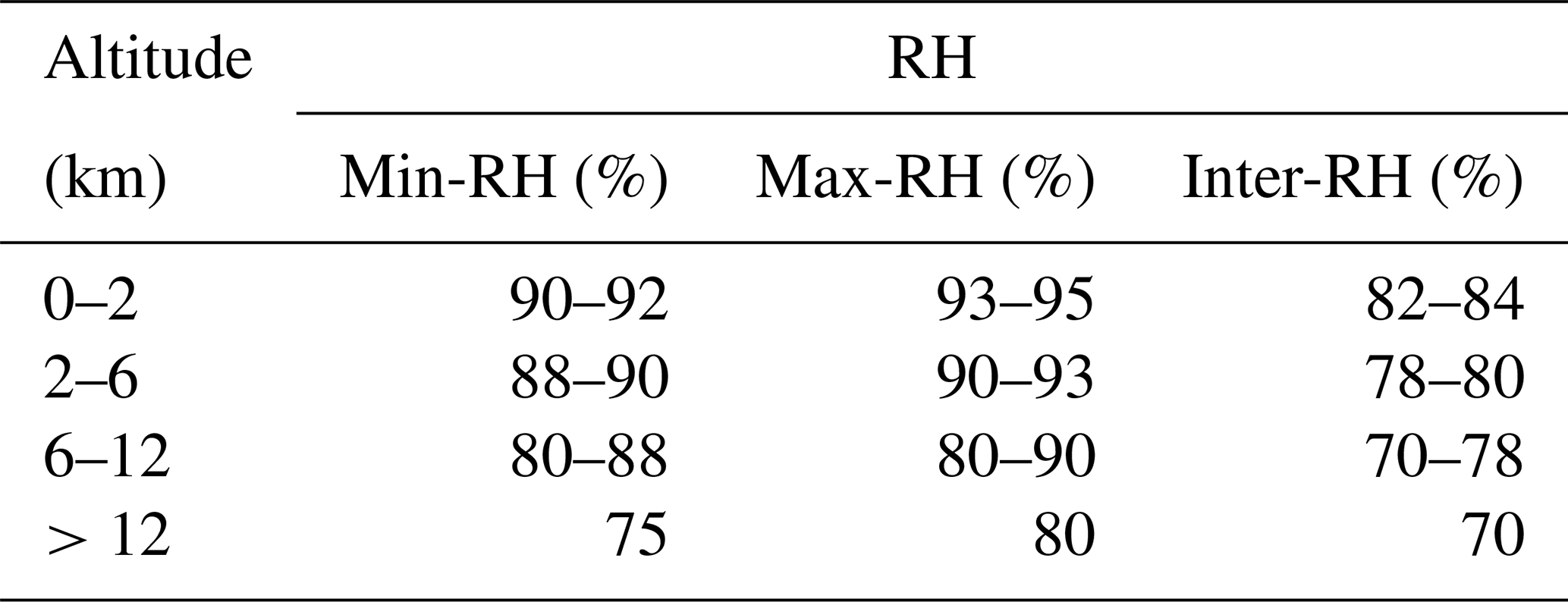
We apply an altitude-dependent relative-humidity thresholding method to identify humidity-defined moist layers associated with cloud structures. Specifically, following the altitude-dependent RH threshold scheme proposed by Zhang et al. (2016), different minimum, maximum, and intermediate RH thresholds are used for different altitude ranges (Table 1). Based on this scheme, we adjust the order of moist-layer identification and merging steps to avoid prematurely discarding thin layers before merging. The processing steps include:

• i.

  remove moist layers with base height < 120 m and cloud geometrical thickness (CGT) < 400 m;

• ii.

  identify moist layers using the altitude-dependent minimum RH threshold;

• iii.

  merge adjacent moist layers when their separation is < 300 m;

• iv.

  remove moist layers with CGT < 30 m.

Radiosondes may drift horizontally by up to approximately 30 km during ascent and therefore cannot be regarded as instantaneous single-column observations. Consequently, radiosonde-derived moist layers are used only as an independent consistency reference rather than as direct supervision or absolute ground truth.

2.6 VDE-based cloud-layer identification product

To improve model generalization across sites and observing conditions, we introduce a conventional cloud-layer identification approach based on elastic lidar echoes – the VDE algorithm (Zhao et al., 2014) – to construct the teacher labels required for the distillation stage. This can be viewed as a single-source, experience-based information stream.

VDE is a physics-informed, rule-based method for cloud-aerosol discrimination, originally developed for cloud-layer identification from single-channel elastic lidar observations. It operates directly on elastic echoes without range-squared correction. Rather than applying a fixed intensity threshold, VDE performs a histogram equalization-like transformation on the vertical distribution of echo intensity, enhancing structural differences and highlighting potential feature layers, as shown in Fig. 2n.

Based on the equalized signal, VDE analyzes salient layers and combines (i) local peak characteristics and (ii) height-dependent attenuation behavior to distinguish clouds from aerosols. Typically, clouds manifest as prominent intensity peaks accompanied by rapid signal decay, especially for optically thick water clouds or low-level clouds. In contrast, aerosol layers tend to show smoother intensity variations and often lack the combined signature of strong peaks and sharp attenuation.

Accordingly, VDE classifies salient layers in each vertical profile: layers with distinct peaks and rapid attenuation are treated as positive samples (cloud), whereas layers with smooth variations and lacking pronounced attenuation are treated as negative samples (aerosol or clear sky). This procedure provides an empirical discrimination mechanism with clear physical intuition.

Building on the conventional binary VDE output, Zou et al. (2024) further extended the decision from hard classification to a discretized cloud-probability representation, where different probability levels are assigned according to peak saliency and attenuation characteristics. This representation partially preserves the uncertainty of cloud/non-cloud decisions and provides a suitable form of weak supervisory information.

As shown in Fig. 2n, VDE identifies the major cloud structures but may produce elevated cloud-probability levels in the lower-middle troposphere under strong aerosol loading, reflecting the limitations of empirical cloud–aerosol discrimination under complex conditions. In this study, the VDE-derived cloud-probability product is not used as the final cloud-layer identification result; instead, it is used only as weak supervision during the distillation stage.

Specifically, VDE is independently applied to the total elastic signals at 355, 532, and 1064 nm, and the cloud-probability outputs from the three wavelengths are averaged to generate the final soft supervisory target. This target provides physically informed guidance for the deep learning model after self-supervised pretraining, encouraging consistency with traditional lidar-based decision logic. We emphasize that VDE is used only during the distillation stage. It is not used in final inference or performance evaluation. Its role is to provide an auxiliary constraint rooted in physical experience, rather than to replace manual annotations or the deep learning model itself.

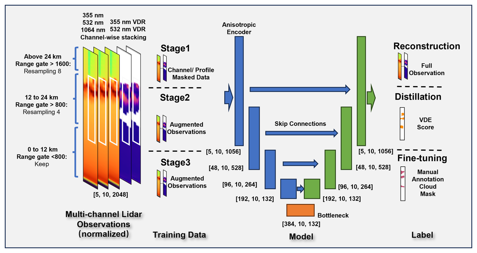
Figure 3 Schematic of the cloud-layer identification network based on multi-channel lidar observations and the three-stage training framework. The three dimensions of [5, 10, 1056] and other vectors correspond to observation channels, temporal profiles, and resampled vertical bins, respectively.

3 Methodology

This section presents the proposed cloud-layer identification method and its training strategy. Motivated by (i) the continuous structural patterns of ground-based lidar observations in the time-height domain and (ii) the pronounced observation shifts across sites and instruments, we model multi-channel lidar measurements as a multi-channel 2D time-height array. We then develop an anisotropic encoder-decoder network together with a three-stage training framework to enable stable identification of cloud-layer structures and to improve cross-site generalization. The overall pipeline is illustrated in Fig. 3. Using multi-channel time-height observations as input, the model is trained under a unified architecture in three consecutive phases: self-supervised reconstruction pretraining, distillation with VDE teacher signals, and fine-tuning with manually refined labels.

This section focuses on problem formulation, network design, and the stage-wise training strategy. Implementation details, hyperparameter settings, and additional experiments are deferred to the Appendix to ensure reproducibility.

3.1 Problem formulation and input representation

Ground-based lidar actively probes the atmosphere in a time-height profiling manner, featuring high vertical resolution and strong temporal continuity. Unlike conventional 2D remote-sensing imagery, the time and height axes are physically asymmetric: the height dimension corresponds to the true vertical atmospheric structure, whereas the time dimension reflects the temporal evolution of atmospheric processes. Therefore, simply treating lidar measurements as an isotropic 2D image and modeling them uniformly is insufficient to capture the underlying physical characteristics.

In this study, multi-wavelength parallel-polarized elastic signals at 355, 532, and 1064 nm and VDR at 355 and 532 nm are stacked along the channel dimension to form a multi-channel time–height input tensor. The model outputs a corresponding binary cloud-layer mask, which marks echo regions associated with cloud processes.

Along the time dimension, the model does not make decisions from a single profile in isolation. Instead, each sample consists of 10 consecutive lidar profiles with a temporal resolution of 5 min, corresponding to a 50 min local observation window, which is comparable to the timescale of many cloud-layer structural variations while remaining robust to operational interruptions and missing observations.

The resulting cloud-layer masks are further converted into operation-relevant geometric products, including cloud-base and cloud-top heights, for the validation analyses in Sect. 4.

3.2 Anisotropic encoder-decoder network architecture

To account for the intrinsic physical asymmetry between the temporal and vertical dimensions of ground-based lidar observations, we design an anisotropic encoder–decoder network based on a U-Net architecture (Fig. 3). In this framework, the encoder extracts hierarchical representations from the time–height input, while the decoder progressively restores spatial resolution to generate pixel-level cloud-layer masks. Unlike conventional image segmentation networks that treat two spatial dimensions equivalently, the proposed architecture explicitly distinguishes temporal continuity from vertical atmospheric structure.

Before entering the network, vertical resampling is applied to adapt the representation scale to the altitude-dependent characteristics of lidar observations. The original lidar profiles contain 2048 vertical range gates with a vertical resolution of 15 m. The vertical dimension is divided into three regions: the lower atmosphere (range gate < 800, approximately 0–12 km), the middle atmosphere (800 ≤ range gate < 1600, approximately 12–24 km), and the upper observation range (range gate ≥ 1600, approximately 24–30.7 km). The lower region retains relatively fine vertical sampling to preserve sharp cloud boundaries and aerosol–cloud transition structures, whereas stronger resampling is applied to the middle and upper regions with factors of 4 and 8, respectively, to reduce redundant vertical information and enlarge the effective representation scale for weaker high-altitude structures. After vertical resampling, the input tensor is transformed from the original [5, 10, 2048] representation to the network input size of [5, 10, 1056], where the three dimensions correspond to observation channels, temporal profiles, and resampled vertical bins, respectively.

The anisotropic feature extraction is further achieved through direction-specific convolutional operations. Kernel sizes are defined as temporal dimension × vertical dimension. Temporal continuity features are extracted using 3 × 1 convolutional kernels, which integrate information along the time axis while preserving vertical resolution. In contrast, vertical atmospheric structures are modeled using height-oriented kernels. Specifically, the initial feature-extraction layer (stem) and the final decoder stage employ 1 × 3 convolutional kernels to preserve fine vertical details. The other encoder and decoder layers, together with the bottleneck block, use 1 × 5 convolutional kernels to increase the vertical receptive field and capture multilayer cloud structures. The bottleneck is the central network block that connects the encoder to the decoder at the coarsest vertical resolution. This factorized anisotropic convolution design enables the network to emphasize vertically coherent atmospheric structures while maintaining local temporal continuity.

No pooling is applied along the temporal dimension throughout the network. The temporal dimension is therefore preserved during feature extraction, allowing the model to utilize short-term continuity information from the 10 consecutive lidar profiles without relying on long temporal sequences. This design improves robustness under operational conditions where missing observations, precipitation interference, strong background radiation, or instrument-state variations may interrupt continuous lidar measurements.

Between the encoder and decoder, skip connections perform joint fusion across scales and channels, transferring multi-scale wavelength- and polarization-dependent features from the encoder to the decoder for recovering fine-grained cloud boundaries (Ronneberger et al., 2015). In addition, gated skip connections are introduced (Oktay et al., 2018; Jiang et al., 2021) to adaptively regulate the transferred features, thereby controlling the contribution of multi-scale and multi-channel information under varying signal-to-noise ratios (SNRs) and cloud–aerosol ambiguity conditions. Specifically, the three gated skip connections employ 1 × 5 height-oriented kernels to selectively weight vertical feature information passed from the encoder to the decoder. This mechanism enables the network to retain informative atmospheric structures while reducing the influence of less reliable features under weak-signal conditions or complex aerosol–cloud coexistence scenarios.

This design preserves the multi-scale representation capability of the U-Net architecture while explicitly supporting multi-channel feature fusion tailored for network-scale lidar observations. By integrating vertical structural information, local temporal continuity, and adaptive feature selection, the proposed architecture is designed to improve the robustness of cloud-layer identification under heterogeneous operational lidar conditions.

3.3 Three-stage training strategy

To improve stability and generalization under limited manual annotations, we adopt a three-stage training strategy (Fig. 3). The first two stages constitute a label-efficient representation learning phase, whereas the final stage performs supervised adaptation using expert-refined annotations. In this study, the term “pretraining” refers to the first two stages, including self-supervised representation learning (Stage 1) and VDE-guided probabilistic distillation (Stage 2). Together, these two stages constitute a physics-guided pretraining phase before supervised fine-tuning with expert annotations (Stage 3).

Stage 1 employs a self-supervised reconstruction task based on channel-wise and profile-wise masking, guiding the model to learn spatiotemporally coherent structures and cross-channel consistency from lidar echoes without requiring manual cloud labels (Vincent et al., 2008; He et al., 2022).

Stage 2 performs VDE-guided probabilistic distillation to further regularize the cloud/non-cloud decision boundary learned from the self-supervised representation. Specifically, discretized cloud-probability levels generated by the conventional VDE algorithm (Zhao et al., 2014; Zou et al., 2024) are used as probabilistic supervisory information rather than absolute ground truth labels, and the segmentation head is optimized on top of the Stage-1 representation. Compared with binary decisions, probability-based guidance provides an uncertainty-aware signal that stabilizes learning under ambiguous conditions, including weak echoes, strong background noise, and aerosol–cloud overlap. In addition, aerosol-labeled regions are explicitly included as non-cloud constraints to penalize aerosol-induced false positives and prevent overly permissive cloud decisions. Overall, Stage 2 introduces physically informed guidance while limiting dependence on dense manual annotations.

Because the VDE-derived probabilities are used as weak supervision during Stage 2, systematic errors in the empirical teacher, such as elevated cloud probabilities under strong aerosol loading, may be partially inherited by the student model. At each time–height pixel, the VDE-derived cloud-probability scores from the 355, 532, and 1064 nm elastic channels are averaged to form the soft supervisory target. The use of these soft targets, explicit aerosol-suppression constraints, and subsequent fine-tuning with expert annotations is intended to reduce the influence of systematic teacher errors, but cannot eliminate it. Stage 3 fine-tunes the model using a small set of manually refined cloud-layer masks. This stage further improves boundary delineation accuracy and cross-site generalization while preserving the stable structural representations learned in the previous stages.

It should be noted that the multi-vendor and multi-site observation configurations in CARLNET inevitably introduce instrument-parameter differences and energy fluctuations in real operations. Rather than treating this heterogeneity as noise to be avoided, we leverage it as a realistic condition for evaluating robustness under varying instrument settings. By incorporating cross-site and cross-time data in the self-supervised and distillation stages, the model is encouraged to learn structural representations that are insensitive to instrument-dependent signal variations and operational fluctuations, thereby improving generalization to unseen sites and different instrument conditions.

3.4 Data augmentation and robustness design

In real-world operations, ground-based lidar observations are inevitably affected by non-ideal factors, including cross-vendor instrument differences, laser energy fluctuations, background-noise variations, and signal perturbations under complex environmental conditions. These factors frequently occur in operational network-scale observations and constitute major sources that limit the cross-site generalization of deep learning models.

In this study, raw lidar signals are resampled to a 5 min temporal resolution in operational processing to balance temporal continuity, signal stability, and computational efficiency for automated cloud-layer identification.

However, the effective time resolution may still differ across sites due to observing conditions, quality control, or missing data. To address this, we introduce a set of lidar-oriented data augmentation strategies during training. Through explicit sampling and perturbation mechanisms, these augmentations cover variations in time scales and observing conditions, thereby improving robustness to time-resolution shifts.

The adopted augmentations operate primarily at the input-observation level, aiming to emulate realistic conditions such as energy-scale variations, noise perturbations, local temporal gaps, and incomplete channel information (Xie et al., 2020). The selected perturbation ranges are determined based on typical variability in operational lidar measurements, including laser-energy fluctuations, photon-counting noise characteristics, and signal-quality variations. These operations encourage the model to focus on structural patterns in the time–height domain rather than relying on specific signal amplitudes or fixed temporal completeness patterns, thereby reducing sensitivity to observation-condition differences.

These augmentation strategies are applied across the three training stages and play important roles during the representation learning and VDE-guided distillation stages. The former facilitates the learning of stable time–height structural representations, whereas the latter further reduces uncertainty in cloud/non-cloud discrimination under noisy and variable observation conditions with physically informed guidance.

All augmentations are applied only during training and are not used during inference or evaluation. Moreover, the augmentation operations are designed to remain physically plausible for lidar observations and do not introduce additional label information. The augmentation types, parameter ranges, and stage-wise usage are summarized in the Appendix.

Once trained and validated, the model can be applied with the same preprocessing and inference protocol to generate consistent cloud-layer masks, cloud-base heights, and cloud-top heights for automated CARLNET processing. These products provide a basis for downstream calibration, quality control, and future long-term cloud-structure analyses, but the present study focuses on method validation and cross-site transferability.

4 Experiments and validation

This section evaluates the proposed framework as an automated cloud-layer identification technique for network-scale Raman lidar processing. The validation is designed to test whether the method can maintain stable performance under cross-site differences in instrument response, background conditions, aerosol environment, and cloud structure. We assess the framework progressively in terms of annotation efficiency, pixel-level identification accuracy, operation-relevant geometric products including cloud-base and cloud-top heights, and external consistency with independent radiosonde observations.

Unless otherwise specified, all evaluations are conducted using continuous observations from three held-out CARLNET sites (51628, 53845, and 58847) in January 2025. These sites are excluded from both the pretraining phase (including Stage 1 self-supervised representation learning and Stage 2 VDE-guided probabilistic distillation) and the supervised fine-tuning stage. Any experiment introducing a small amount of test-site annotations is treated separately as a test-site adaptation experiment and is not included in the main validation protocol. The VDE method is used as the conventional physics-based baseline throughout this section.

The results reported in Figs. 4–6 and Tables 2–3 were obtained from a single training run using the fixed experimental configuration described in Appendix A. They are therefore interpreted as deterministic performance estimates for the specified data split rather than as statistical estimates of variability across model initializations.

4.1 Data-size test-site adaptation experiment

To evaluate the performance of different training strategies under limited manual annotations, we conducted a test-site adaptation experiment using varying amounts of labeled training data. Figure 4 compares four strategies: direct supervised training, Stage 1 only (self-supervised representation learning), Stage 2 only (VDE-guided probabilistic distillation), and Stage 1 + Stage 2 (physics-guided pretraining). The x-axis indicates the number of consecutive observation days used for training, while the y-axis reports the F1 score evaluated on the fixed independent test set. The definition and computation of the F1 score are provided in Appendix A. The test set comprises continuous observations collected in January 2025 from the three test sites, ensuring independence between the training and test data in both time and site.

As shown in Fig. 4, under the small-sample setting of 10 labeled training days, both Stage 1 and Stage 2 improve performance relative to direct supervised training, while the complete Stage 1 + Stage 2 strategy provides the largest gain. Specifically, the F1 score increases from approximately 0.75 for direct supervised training to approximately 0.91 with the complete physics-guided pretraining strategy, indicating a substantial reduction in segmentation error. As the amount of labeled training data increases, all four strategies show improved performance but diminishing marginal gains, with their F1 scores approaching a plateau at approximately 40 labeled days.

This experiment demonstrates that the combination of self-supervised representation learning and VDE-guided probabilistic distillation improves annotation efficiency by enabling competitive performance with fewer manually annotated observations. Considering the trade-off between annotation effort and marginal performance improvement, approximately 40 training days are selected for subsequent experiments. While F1 score provides an overall assessment of pixel-level cloud-layer identification capability, the practical advantages of improved representation learning are further reflected in cloud-boundary localization and robustness under complex observation conditions. Therefore, the impact of different training strategies on operationally relevant cloud-base and cloud-top height estimation is evaluated in Sect. 4.2.2, while qualitative analyses under challenging cloud–aerosol conditions are presented in Sect. 4.2.3.

Figure 4 Comparison of cloud-layer identification performance (F1 score) under different training-data scales. Colours, line styles, and marker shapes distinguish the training strategies. The grey dashed vertical line marks the selected 40 d training size, beyond which additional annotations yield limited marginal improvement in F1 score.

Overall, the results suggest that pretraining not only reduces reliance on large-scale manual annotations for cloud-layer identification, but also reduces reliance on extensive manual annotations for cross-site deployment.

4.2 Cross-site overall performance

4.2.1 Overall performance and clarification of test-site usage

Table 2 reports the overall performance under different training strategies and different usages of the test-site data. Metrics include intersection over union (IoU), F1 score, precision, and recall. All results are computed over the full test set. Early stopping was applied using the validation criterion described in Appendix A5.

In Table 2, “Test-site observations used in pretraining” indicates whether observations without expert annotations from the three held-out test sites were included in Stage 1 and Stage 2, whereas “Test-site annotations used in fine-tuning” indicates whether a limited amount of manually annotated data from each test site was introduced during Stage 3. Specifically, the test-site adaptation setting uses 2 annotated days per site sampled from 2024, which are temporally independent of the January 2025 test period. The configuration excluding both test-site observations from pretraining and test-site annotations from fine-tuning represents the primary strict cross-site and cross-time evaluation.

As shown in Table 2, pretraining (Stage 1 and Stage 2) yields stable gains in cross-site evaluation. Under the strict setting where no test-site observations are introduced during either pretraining or fine-tuning, the complete physics-guided pretrained model achieves F1 =0.937, higher than 0.928 obtained by direct supervised training. Measured by inconsistency (1− F1), pretraining reduces it from 0.072 to 0.063, corresponding to a 12.5 % relative reduction. Because the results are obtained under a fixed dataset split and training configuration, the F1 difference should be interpreted as a modest deterministic performance gain rather than formal evidence of statistical significance. Its practical relevance is further evaluated using cloud-boundary errors and qualitative cases in the following sections. Notably, introducing a small amount of test-site annotations during fine-tuning does not further improve performance substantially (F1 =0.935), suggesting that the major benefit primarily comes from transferable structural representations acquired during pretraining rather than from supervised fitting to specific test sites.

Compared with the proposed physics-guided pretrained model, the conventional VDE baseline exhibits lower consistency with manual annotations, particularly under complex cloud structures and strong aerosol backgrounds.

Table 2 Cloud-layer identification performance under different training strategies and different usages of test-site data.

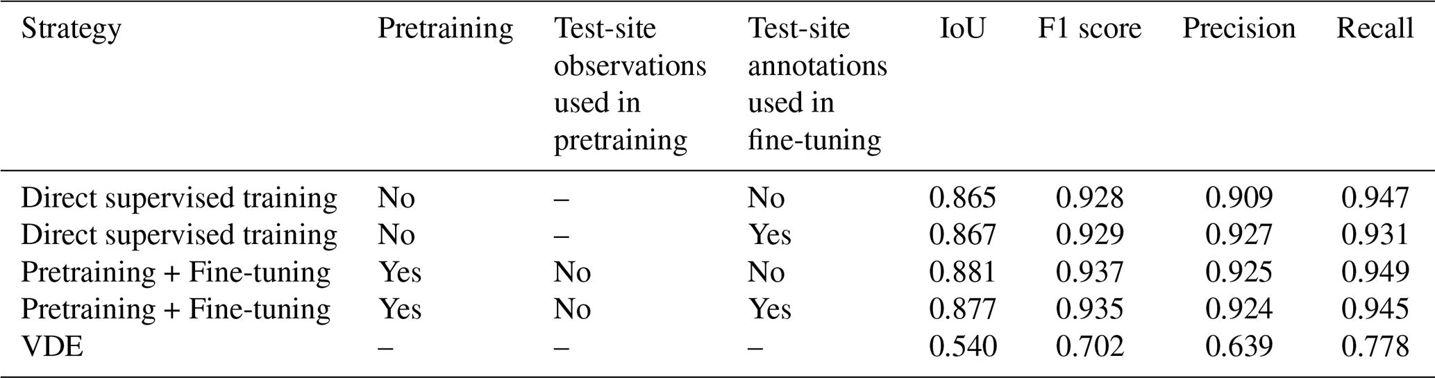
Overall, the results indicate that pretraining provides consistent improvements and the strictest configuration performs no worse than configurations that include test-site information, supporting that the performance gain does not originate from site-specific fitting. This suggests that pretraining primarily enhances the model's general representation of cloud-layer structures, offering a more reliable foundation for operational scaling.

4.2.2 Operation-relevant evaluation: cloud-base and detectable cloud-top heights

The operational value of a cloud-layer mask is not only reflected by pixel-level classification accuracy, but also by its capability to characterize cloud geometrical structures, particularly the accurate estimation of cloud-base and cloud-top heights. To evaluate the practical relevance of different methods, predicted cloud-layer masks are converted into geometric cloud products and compared with manually refined annotations.

To derive layer-wise geometric errors, reference and predicted cloud layers are extracted from each vertical profile as vertically contiguous cloud-positive regions. Only layers with a geometrical thickness of at least 90 m are retained, and all eligible layers are evaluated. The lowest and highest cloud-positive range bins of each retained layer define its cloud-base and detectable cloud-top heights, respectively.

Predicted and reference layers are matched using global one-to-one assignment based on the Hungarian algorithm (Kuhn, 1955). The matching cost prioritizes vertically overlapping layer pairs, using vertical intersection over union as the primary criterion and absolute layer-center separation as a secondary criterion. For non-overlapping layers, matching is permitted only when their minimum vertical separation does not exceed 300 m. Each predicted or reference layer can be assigned to at most one counterpart. Unmatched reference layers are counted as missed detections, whereas boundary errors are calculated only for successfully matched pairs. The 300 m criterion restricts candidate-layer separation; no additional rejection threshold is applied to the boundary errors of successfully matched pairs.

The statistics reported in Fig. 5 and Table 3 are calculated using all successfully matched layer pairs. For visualization, Fig. 5 displays a random subset of at most 2000 pairs per method, selected using a fixed random seed of 42. This plotting subsample does not affect the reported statistics.

Because ground-based lidar signals may be strongly or completely attenuated by optically thick clouds, the reported cloud-top height refers to the highest cloud boundary supported by a detectable lidar return, rather than necessarily the physical upper boundary of the cloud. Reliable cloud-top estimation therefore requires sufficient residual signal and signal-to-noise ratio near the upper cloud boundary. When complete attenuation prevents observation of the physical cloud top, the corresponding reference boundary is defined by the highest detectable cloud-positive bin in the manually refined mask. Cloud layers that are completely obscured and produce no detectable lidar return cannot be included in the boundary-error evaluation.

Figure 5 presents the correspondence between estimated cloud boundaries and manually refined annotations, while Table 3 summarizes the detection rate and quantitative errors of cloud-base and cloud-top heights. For cloud-base estimation, the pretrained model achieves an MAE of 59.1 m, which is comparable to the direct supervised model (55.3 m) and substantially better than the VDE baseline (123.6 m). The corresponding cloud-base bias is −12.8 m, which is smaller than the original 15 m vertical sampling interval of the lidar and is therefore negligible at the native instrumental resolution. This indicates that all deep learning models can effectively capture relatively strong cloud-base signatures once sufficient structural information is learned.

The advantage of pretraining is more evident for cloud-top estimation. The pretrained model achieves a cloud-top MAE of 82.2 m, reducing the error by approximately 12.6 % compared with direct supervised training (94.0 m) and by approximately 67 % compared with VDE (250.7 m). This improvement suggests that the proposed pretraining strategy enhances the preservation of weak and optically thin cloud boundaries, where accurate cloud-top identification is more challenging due to signal attenuation, low signal-to-noise ratio, and multilayer cloud structures.

Beyond geometric errors, Table 3 also reports the cloud detection rate. The pretrained and direct supervised models exhibit nearly identical detection rates (93.9 % and 94.1 %, respectively), indicating that the improvement from pretraining does not originate from simply detecting more cloud layers. Instead, the main benefit lies in more accurate delineation of cloud boundaries and vertical structures. In contrast, VDE shows a lower detection rate (86.0 %) and substantially larger geometric errors, demonstrating its limitations under complex network-scale observations.

The larger cloud-top errors of VDE can be attributed to the empirical threshold-based discrimination strategy. As shown in Fig. 5c and f, VDE exhibits stronger deviations from the manually refined boundaries, particularly for cloud-top estimation. The attenuation-based decision criteria may suppress weak cloud signals near cloud boundaries, leading to underestimated cloud-top heights and missing thin or weak-echo cloud structures.

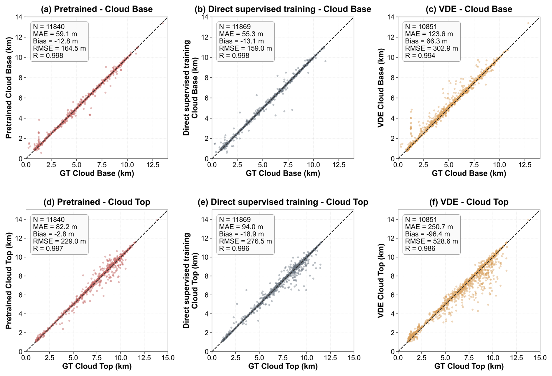
Figure 5 Comparison of estimated cloud-base and detectable cloud-top heights with manually refined annotations. Panels (a)–(c) show cloud-base comparisons, and panels (d)–(f) show detectable cloud-top comparisons. Panels (a), (d), (b), (e), and (c), (f) correspond to the pretrained model, direct supervised model, and VDE method, respectively. GT denotes the manually refined reference, N is the number of successfully matched cloud layers, MAE is the mean absolute error, bias is the mean signed error defined as prediction minus reference, RMSE is the root-mean-square error, and R is the Pearson correlation coefficient. The dashed diagonal line indicates perfect 1:1 agreement. All statistics are calculated from the complete set of successfully matched layer pairs. For visualization, at most 2000 pairs per method are randomly selected.

Taken together, these results demonstrate that the advantage of the proposed pretraining strategy is primarily reflected in improved cloud-boundary localization rather than a simple increase in cloud occurrence detection. The improved cloud-top estimation indicates stronger capability in preserving vertically extended and weak cloud structures, which is important for operational lidar cloud processing, quality control, and cloud-structure characterization.

Table 3 Quantitative comparison of detection rate and cloud-base/cloud-top height errors across methods. MAE denotes mean absolute error.

4.2.3 Qualitative examples under complex conditions

To further illustrate the role of physics-guided pretraining in improving structural stability, Fig. 6 presents qualitative comparisons between the Stage 1 + Stage 2 pretrained model and the direct supervised model under complex lidar observation conditions. The examples focus on challenging scenarios including weak-echo clouds, aerosol–cloud coexistence, signal fluctuations, and multilayer structures. Compared with direct supervised training, the pretrained model produces cloud-layer masks that better agree with manually refined annotations in terms of boundary continuity, weak-layer preservation, and temporal consistency.

Figure 6a shows an example from Fuzhou (58847), where a weak aerosol layer exists above the boundary layer during 10:00–18:00 UTC. Under this aerosol background, the direct supervised model tends to misclassify weak scattering structures as cloud, resulting in unrealistic continuous cloud regions (black box). In contrast, the pretrained model suppresses aerosol-induced false detections more effectively and maintains more physically consistent cloud boundaries. This example demonstrates the benefit of learning transferable structural representations for distinguishing cloud signals from aerosol-related echoes.

Together, these examples demonstrate that the advantage of physics-guided pretraining is not limited to improvements in average segmentation metrics, but is reflected in more stable structural interpretation under challenging observation conditions. Combined with the detection-rate analysis and geometric evaluation, the results suggest that the proposed framework improves the representation of complex cloud structures, particularly under weak echoes, aerosol–cloud coexistence, and variable operational conditions.

Figure 6 Qualitative comparison of cloud-layer masks produced by pretrained and direct supervised models under complex echo conditions. The background shows the 1064 nm elastic channel (10:00–18:00 UTC; 0–6 km). The black solid contour denotes the pretrained model, whereas the black dotted contour denotes the direct supervised model. Red boxes highlight representative regions with substantial differences. Panel (a) shows Fuzhou (58847, 13 January 2025), and panel (b) shows Aksu (51628, 28 January 2025).

4.3 Independent validation with radiosonde observations

The radiosonde-based evaluation includes 47 valid lidar–radiosonde comparison cases from all three independent test sites. The quantitative statistics reported in Table 4 are calculated by aggregating the matched cases from Aksu, Yan'an, and Fuzhou. Figures 7 and 8 present representative examples from Aksu to illustrate the comparison procedure and typical differences among the proposed model, VDE, manual annotations, and radiosonde-derived moist layers.

Considering the temporal and spatial mismatch between lidar observations and radiosonde profiles, we aggregate lidar-derived cloud-layer masks within ± 1 h around each radiosonde launch time and compare the resulting cloud structures with radiosonde-identified moist layers. This temporal aggregation is adopted to account for the time-evolving nature of cloud systems and the fact that radiosondes sample the atmosphere along a drifting ascent trajectory rather than an instantaneous vertical column.

For Aksu (Fig. 7), the proposed model and VDE show generally consistent temporal and vertical evolution of major cloud processes, while both exhibit systematic differences from radiosonde-derived moist layers in cloud boundaries. These differences mainly arise from the distinct observing principles: lidar provides high-resolution backscatter observations and is sensitive to weak scattering structures, whereas radiosonde-based cloud identification relies on altitude-dependent humidity thresholds and samples the atmosphere along a drifting ascent trajectory. On this basis, the proposed model tends to better preserve the continuity of high-level weak-echo structures (Fig. 7b), with fewer apparent temporal discontinuities than VDE, which helps mitigate cloud-top underestimation for tenuous upper-level layers. For low-level clouds, both methods capture the major structures reasonably well, with relatively smaller differences compared with upper-level weak clouds (Fig. 7c).

Figure 8a and b provide zoom-in comparisons of representative periods under radiosonde constraints. In these cases, the proposed model generally maintains closer vertical continuity with the radiosonde-derived cloud layers, while VDE exhibits larger deviations or intermittent discontinuities in weak-signal regions. These differences are particularly evident for cloud boundaries with relatively weak backscatter signals, where empirical threshold-based methods are more susceptible to local signal fluctuations. The consistency observed in these examples supports the quantitative comparison in Table 4 and indicates that the proposed model provides more stable structural representation under challenging lidar observation conditions.

Beyond these qualitative comparisons, we further quantify the consistency between lidar-derived cloud layers and radiosonde-identified moist layers as shown in Table 4. Because radiosonde-based identification is affected by humidity thresholds, ascent sampling, and spatial drift, these statistics are interpreted as structural consistency indicators rather than strict accuracy measurements. The proposed model achieves a structural consistency rate of 38.3 %, higher than VDE (34.0 %) and expert annotation (27.7 %). These differences should not be interpreted as absolute accuracy differences, because radiosonde-derived moist layers and lidar-observed cloud layers represent different atmospheric properties and are affected by different sampling characteristics. Instead, the structural consistency rate reflects the agreement between the two observing systems.

In summary, independent radiosonde-based comparisons indicate that the proposed model (DL) and VDE are broadly consistent in the temporal evolution of major cloud processes. Under the systematic offsets expected from differing observing principles, the proposed model shows improved consistency for high-level, weak-echo layers, typical of thin cirrus, and for multilayer scenes, by preserving layer continuity and reducing intermittent misses relative to VDE. This behavior aligns with the reduced cloud-top errors and the qualitative examples under complex echoes, and supports the interpretation that pretraining mainly improves structural stability and physically consistent cloud-layer representation , rather than simply increasing cloud detections or yielding isolated metric gains.

We note that radiosonde-based cloud identification is derived from altitude-dependent relative-humidity thresholds and is therefore subject to uncertainties associated with threshold selection, moist-layer merging criteria, and horizontal drift during ascent. Consequently, radiosonde observations are not treated as a strict quantitative ground truth for lidar cloud-layer identification. Instead, they provide an independent atmospheric reference for evaluating the consistency of identified cloud-layer structures, including layer altitude, continuity, and multilayer occurrence.

Figure 7 Consistency analysis of cloud-layer identification at Aksu (51628, January 2025) under radiosonde constraints. Panel (a) shows the radiosonde moist-layer cloud structure; panel (b) shows the manually refined labels; panel (c) shows the difference map between the proposed model and the VDE method (green: both; red: DL only; yellow: VDE only). Radiosonde-derived moist layers are used only as an independent structural-consistency reference and not as ground-truth cloud boundaries.

Table 4 Consistency of lidar-derived cloud layers with radiosonde-identified moist layers based on 47 valid comparison cases from the three independent test sites.

Figure 8 Zoom-in examples of lidar-derived cloud-layer identification under radiosonde constraints. The 1064 nm elastic signal is shown as the background, with overlays of the proposed model, VDE-derived cloud layers, and radiosonde-identified moist layers. The black solid line denotes the proposed model, the black dotted line denotes the VDE result, and the gray dashed line denotes the radiosonde-derived moist layer. Radiosonde-derived moist layers are shown only as an independent structural-consistency reference and are not treated as ground-truth cloud boundaries.

5 Conclusion and Discussion

This study developed and validated a multi-channel cloud-layer identification framework with reduced dependence on absolute calibration for automated Raman lidar network processing. The framework operates directly on observation-level elastic signals at 355, 532, and 1064 nm and volume depolarization ratios at 355 and 532 nm, without relying on fine-grained optical retrieval products as model inputs. By combining a lidar-specific anisotropic encoder-decoder architecture with self-supervised pretraining, VDE-guided probabilistic distillation, and supervised fine-tuning with limited expert-refined labels, the proposed method is designed to improve cloud-boundary stability, multilayer preservation, and cross-site transferability under realistic operational perturbations.

The framework was evaluated under a strict cross-site and cross-time setting using continuous observations from three held-out CARLNET sites that were excluded from both pretraining and supervised training. The results show that physics-guided pretraining improves pixel-level cloud-layer identification evaluation, while reducing dependence on extensive manual annotations. Compared with training from scratch, the F1 score increases from 0.928 to 0.937, corresponding to a 12.5 % relative reduction in inconsistency (1− F1). The labeled-data-size adaptation experiment further demonstrates improved annotation efficiency, with the model approaching a performance plateau using a limited number of manually refined training days. These results indicate that the main benefit of pretraining is not site-specific fitting, but the acquisition of transferable time-height and cross-channel representations.

From an operational perspective, the improvement is more evident in geometry-related products. Compared with direct supervised training, the pretrained model achieves comparable cloud-base height estimation while reducing cloud-top height error by approximately 12.6 %. Relative to the conventional VDE baseline, the reduction in cloud-top error is particularly pronounced, with cloud-top MAE decreasing from 250.7 to 82.2 m. The detection rates of the pretrained and direct supervised models remain nearly identical (93.9 % vs. 94.1 %), indicating that the performance gain mainly arises from improved cloud-boundary localization and multilayer structure preservation rather than from simply increasing cloud detections. Qualitative cases further show that the pretrained framework suppresses aerosol-induced false detections and reduces spurious responses associated with short-term signal fluctuations.

Independent radiosonde-based comparisons provide an additional consistency check from a different observing system. Although lidar and radiosonde cloud indications are not expected to match exactly because of differences in observing principles, humidity-threshold uncertainty, and balloon drift, the proposed framework shows higher structural consistency with radiosonde-identified moist layers than both expert annotation and VDE. Specifically, the proposed model achieves a structural consistency rate of 38.3 %, compared with 34.0 % for VDE and 27.7 % for expert annotation. This result should not be interpreted as an absolute accuracy comparison, but rather as evidence that the proposed framework provides a more consistent representation of atmospheric layer structures under independent observational constraints.

This advantage is particularly relevant for high-level weak echoes and multilayer scenes, where empirical methods may experience larger uncertainty in maintaining layer continuity. For first-layer clouds dominated by stronger low-level echoes, the difference between the proposed method and VDE is smaller, suggesting that the primary practical value of the proposed framework lies in improving structural completeness under weak-signal and multilayer conditions.

Several limitations should be noted. First, the present framework focuses on cloud-layer identification and does not explicitly separate precipitation from cloud layers. Scenes affected by precipitation, virga, or strongly attenuating hydrometeors may require additional physical constraints or task-specific labels. Second, although the model is designed to reduce dependence on absolute calibration, its inputs remain affected by near-range overlap, daytime background radiation, signal saturation, and severe attenuation by optically thick low clouds. These factors may still limit the observability of certain cloud regions, especially near the blind zone and above persistent low clouds. In particular, the model cannot recover a physical cloud top when the lidar signal is fully attenuated below that boundary. Third, the model uses a short temporal context window and is not designed to depend on long temporal averaging; however, its behavior under highly irregular sampling, sparse observations, and prolonged data gaps still requires further systematic evaluation. Fourth, although the current validation uses strict held-out sites within CARLNET, broader tests on external lidar networks are needed to assess cross-instrument and cross-platform generalizability. In addition, the current evaluation focuses on deterministic model performance under a fixed experimental setting. Although consistent improvements are observed across pixel-level metrics, geometric products, qualitative cases, and radiosonde-based consistency analyses, future work should further quantify uncertainty arising from model initialization and training variability through repeated experiments and confidence estimation.

Future work will focus on improving inference-time robustness and engineering readiness under challenging operational conditions, including strong daytime background, frequent low-cloud attenuation, irregular sampling, and data gaps. The framework will also be extended to external ground-based lidar networks and compared with spaceborne lidar observations to further evaluate cross-platform consistency. In addition, the resulting cloud-layer products can provide a unified basis for downstream calibration, quality control, aerosol-cloud optical retrieval, and future long-term cloud-structure analyses. The training and inference framework, together with pretrained models, will be made available where possible to support reproducible evaluation and broader deployment.

Appendix A

This appendix summarizes the training protocol of the proposed cloud-layer identification framework, including preprocessing, augmentation, model configuration, optimization, and evaluation settings. Unless explicitly stated, the same preprocessing and augmentation pipeline is applied across all stages to ensure consistent learning signals and to facilitate reproducibility.

A1 Preprocessing of multi-channel time-height observations

We distinguish input vertical resampling from architectural anisotropy. Vertical resampling is performed before network input to reduce computational cost, whereas the network architecture applies downsampling only along the height axis.

The three elastic input channels comprise the parallel-polarized signals at 355 and 532 nm and the elastic signal at 1064 nm. These channels are normalized using fixed, instrument-specific and channel-specific median and median absolute deviation (MAD) statistics. For each instrument, the statistics are estimated from a pooled sample of finite, positive elastic-signal measurements from its observation records, before range-squared correction and logarithmic transformation. The resulting scalar statistics are held fixed across input windows and are not recalculated independently for each time–height sample. The normalized elastic signal is defined as

$$\begin{array}{}\text{(A1)}& {\stackrel{\mathrm{̃}}{P}}_{s,c}(t,z)={\displaystyle \frac{\mathrm{1}}{\mathrm{2}}}\left({\displaystyle \frac{P_{s,c}(t,z)-m_{s,c}}{\mathrm{4}{d}_{s,c}+\mathit{ϵ}}}+\mathrm{1}\right),\mathit{ϵ}={\mathrm{10}}^{-\mathrm{8}}\end{array}$$

here, s, c, t, and z index the instrument, elastic channel, temporal profile, and vertical range bin, respectively. The quantities $P_{s,c}\left(t,z\right)$ and $\stackrel{\mathrm{̃}}{P_{s,c}}\left(t,z\right)$ denote the signal values before and after normalization. For the pooled sample S_s,c, the fixed median is $m_{s,c}={\mathrm{median}}_{p\in S_{s,c}}\left(p\right)$, and the MAD is $d_{s,c}={\mathrm{median}}_{p\in S_{s,c}}\left|p-m_{s,c}\right|$, where p denotes an individual signal measurement in the pooled sample. The factor 4 sets the normalization scale, and ϵ ensures a nonzero denominator. The normalized elastic values are not clipped to [0,1].

Following normalization, the three elastic channels undergo range-squared correction and natural-logarithmic compression to reduce dynamic range while preserving structural contrast:

$$\begin{array}{}\text{(A2)}& X_{s,c}(t,z)=\ln (\mathrm{1}+{\stackrel{\mathrm{̃}}{P}}_{s,c}(t,z\left)R_z^{\mathrm{2}}\right).\end{array}$$

Here, $X_{s,c}\left(t,z\right)$ denotes the processed elastic-channel input, R_z is the range expressed in kilometres. The cross polarized channels do not undergo MAD normalization, range-squared correction, or logarithmic transformation. Their ratio values are clipped to [0,1] before network input. The same fixed normalization and deterministic input-processing steps are applied throughout training, validation, and inference. Deployment at a new instrument requires its own normalization statistics, estimated using signal preprocessing and temporal averaging consistent with those used for inference.

To reduce computational cost while preserving the vertical structures relevant to cloud-layer identification, vertical resampling is performed before the observations are fed into the network. Starting from the original 2048 range gates with a vertical resolution of 15 m, the near-range region (range gate index <800, approximately 0–12 km) is retained at the original resolution, while progressively coarser sampling is applied to higher-altitude regions. Specifically, average pooling is applied along the height dimension with a vertical resampling factor of 4 in the middle region (800≤ range gate index < 1600, approximately 12–24 km) and 8 in the upper region (range gate index ≥ 1600, approximately 24–30.7 km). Each non-overlapping group of four or eight adjacent range bins is replaced by its arithmetic mean, while the temporal and channel dimensions remain unchanged. This preprocessing step converts the original 2048 vertical bins into the resampled input representation shown in Fig. 3 ([5, 10, 1056]). The same vertical resampling procedure is applied during all training stages and inference.

The vertical resampling strategy prioritizes preserving lower-atmospheric structures where cloud boundaries and aerosol–cloud interactions are most frequently observed, while progressively reducing redundancy at higher altitudes where the original fine resolution produces high computational costs.

A2 Data augmentation for operational robustness

Operational lidar observations are affected by instrument-to-instrument differences, laser energy fluctuations, background noise variability, and occasional data irregularities. To encourage the model to learn structural cues rather than relying on absolute amplitude scales or specific sampling patterns, we adopt a strong but physically plausible augmentation policy throughout training. Concretely, we apply (i) random height cropping with probability 0.3 using a crop ratio sampled from [0.7, 0.9], (ii) additive Gaussian noise with probability 0.3 and standard deviation 0.05, (iii) multiplicative signal scaling with probability 0.3 using a factor sampled from [0.9, 1.1], and (iv) spatial dropout with probability 0.2 that randomly zeroes 10 % of pixels. These perturbations are applied only to the input observations and do not introduce any additional label information.

All perturbations are applied after channel-wise normalization. Therefore, the Gaussian-noise standard deviation of 0.05 is expressed on the normalized signal scale and corresponds to 5 % of the robust unit scale. The multiplicative scaling range of 0.9–1.1 represents signal-amplitude variations of up to ± 10 %. A cropping ratio of 0.7–0.9 means that 70 %–90 % of the original vertical extent is retained, after which the cropped input is zero-padded to restore the original input size. Spatial dropout removes 10 % of input pixels when activated, simulating localized missing or corrupted observations. These parameter ranges were selected empirically using training-site observations and validation performance to approximate realistic operational variability without generating physically implausible lidar structures. No held-out test-site data were used for parameter selection.

A3 Unified model configuration

A single unified anisotropic encoder-decoder network is used across all experiments. The input is a five-channel time–height tensor comprising parallel-polarized elastic signals at 355, 532, and 1064 nm, and the volume depolarization ratios at 355 and 532 nm. The segmentation head outputs a one-channel cloud-layer mask (cloud vs. non-cloud). The model uses a base width of 48 channels with dropout rate 0.1 and a vertical convolution kernel size k_Z=5. The overall parameter count is approximately 4.28M. A reconstruction head is enabled only in Stage 1 (see below) to reconstruct all five channels; it is removed in Stage 2 and Stage 3 when training focuses on cloud-layer identification.

A4 Stage-wise objectives

Training follows the three-stage strategy described in the main text.

Stage 1 (self-supervised representation learning). The model is pretrained without manual annotations using a multi-task reconstruction objective designed to capture spatiotemporal continuity and cross-channel consistency in time-height echoes. The objective combines: (i) a full-channel reconstruction loss L_recon implemented as MSE over all channels, (ii) a channel-masking prediction loss L_ch where 1–2 channels are randomly masked and reconstructed, and (iii) a temporal-frame prediction loss L_t where one time frame is masked and predicted from its neighbors. This stage encourages a transferable representation that is less sensitive to site-specific scaling and short-term perturbations.

The overall Stage-1 objective is defined as

$$\begin{array}{}\text{(A3)}& {\mathcal{L}}_{\mathrm{Stage}\mathrm{1}}={\mathit{\lambda }}_{\mathrm{recon}}{\mathcal{L}}_{\mathrm{recon}}+{\mathit{\lambda }}_{\mathrm{ch}}{\mathcal{L}}_{\mathrm{ch}}+{\mathit{\lambda }}_t{\mathcal{L}}_t.\end{array}$$

Here, ℒ_Stage1 denotes the total Stage-1 training loss. The terms ℒ_recon, ℒ_ch, and ℒ_t denote the full-channel reconstruction loss, masked-channel prediction loss, and masked temporal-frame prediction loss, respectively. Their corresponding weighting coefficients are λ_recon, λ_ch, and λ_t.

During channel masking, one or two of the five input channels are randomly masked, corresponding to a masking ratio of 20 %–40 %. During temporal prediction, one of the ten input profiles is masked, corresponding to a temporal masking ratio of 10 %. The loss weights are set to ${\mathit{\lambda }}_{\mathrm{recon}}=\mathrm{1},{\mathit{\lambda }}_{\mathrm{ch}}=\mathrm{0.5}$ and λ_t=0.5 throughout Stage 1.

Stage 2 (VDE-guided probabilistic distillation). Starting from the Stage-1 initialization, we inject physical heuristics via distillation using discretized VDE-derived cloud probability as a teacher signal. We employ a weighted BCE-with-logits loss with a positive class weight pos_weight=19.0 (reflecting an average cloud fraction of approximately 5 %). Two additional terms are introduced to improve robustness under operational artifacts. Regions with a low teacher cloud score ≤0.4 receive an aerosol-suppression penalty with a weight of 3.0 to reduce aerosol-induced false positives. Predictions within the first 30 range bins (approximately 0–450 m and within the approximate 500 m incomplete-overlap region) receive a blind-zone penalty with a weight of 15.0 to discourage non-physical cloud detections. The overall Stage-2 objective is defined as

$$\begin{array}{}\text{(A4)}& {\mathcal{L}}_{\mathrm{Stage}\mathrm{2}}={\mathcal{L}}_{\mathrm{BCE}}+\mathrm{3}{\mathcal{L}}_{\mathrm{aero}}+\mathrm{15}{\mathcal{L}}_{\mathrm{blind}}\end{array}$$

where

$$\begin{array}{}\text{(A5)}& {\mathcal{L}}_{\mathrm{BCE}}=-{\displaystyle \frac{\mathrm{1}}{N}}\sum _{i=\mathrm{1}}^N\left[w_{+}{y}_i\log \mathit{\sigma }\left(z_i\right)+(\mathrm{1}-y_i)\log \left(\mathrm{1}-\mathit{\sigma }\left(z_i\right)\right)\right],\end{array}$$

here, ℒ_Stage2 denotes the total Stage-2 training loss, and ℒ_BCE denotes the weighted binary cross-entropy loss. The aerosol-suppression term ℒ_aero penalizes cloud predictions in regions with low VDE-derived cloud scores, whereas the blind-zone term ℒ_blind penalizes cloud predictions within the first 30 range bins. The coefficients 3 and 15 are the respective penalty weights. The weighted binary cross-entropy loss is defined as

where N denotes the total number of pixels, z_i is the raw model logit for pixel i, σ(⋅) denotes the sigmoid function, $y_i\in \left[\mathrm{0},\mathrm{1}\right]$ is the VDE-derived soft target, and $w_{+}=\mathrm{19.0}$ is the positive-class weight. BCE-with-logits applies binary cross-entropy directly to the raw logits, with the sigmoid transformation incorporated internally for improved numerical stability. The positive-class weight was determined from the approximately 5 % cloud-pixel fraction in the training data, corresponding to a negative-to-positive ratio of approximately $(\mathrm{1}-\mathrm{0.05})/\mathrm{0.05}=\mathrm{19}$. The aerosol-suppression and blind-zone weights of 3.0 and 15.0, respectively, were empirically selected using the validation subset from the training sites to balance aerosol-related false positives and non-physical predictions within the near-range blind zone. The held-out test sites were not used for hyperparameter selection, and all weights were fixed for the subsequent experiments.

Stage 3 (supervised fine-tuning with manual annotations). Finally, the model is fine-tuned using a limited amount of manually refined cloud-layer annotations. Stage 3 uses the same weighted BCE-with-logits formulation with $w_{+}=\mathrm{19.0}$, but the soft VDE targets are replaced by binary expert annotations. This stage refines cloud-boundary placement while preserving the robust structural representations learned in Stages 1 and 2.

A5 Optimization schedule and freezing strategy

All stages are optimized using AdamW (Loshchilov and Hutter, 2019). Stage 1 uses a learning rate of $\mathrm{5}\times {\mathrm{10}}^{-\mathrm{5}}$ with weight decay $\mathrm{1}\times {\mathrm{10}}^{-\mathrm{4}}$, batch size 8, and 20 epochs. Stage 2 is trained in two consecutive phases to reduce overfitting to weak supervision: Phase 2A runs for 15 epochs with learning rate $\mathrm{5}\times {\mathrm{10}}^{-\mathrm{5}}$ and weight decay $\mathrm{1}\times \mathrm{10}-\mathrm{4}$ while freezing the first two encoder blocks; Phase 2B runs for 15 epochs with learning rate $\mathrm{2}\times {\mathrm{10}}^{-\mathrm{5}}$ and weight decay $\mathrm{1}\times {\mathrm{10}}^{-\mathrm{5}}$ while freezing the entire encoder (decoder-only adaptation). Stage 3 fine-tuning runs for 40 epochs using learning rate $\mathrm{1}\times {\mathrm{10}}^{-\mathrm{5}}$, weight decay $\mathrm{5}\times {\mathrm{10}}^{-\mathrm{4}}$, batch size 4, and a cosine annealing schedule with ${\mathit{\eta }}_{\min }={\mathrm{10}}^{-\mathrm{6}}$ while freezing the encoder and bottleneck to focus adaptation on the decoder and prediction head. The cosine annealing schedule gradually decreases the learning rate from its initial value to (η_min) following a cosine curve, allowing relatively larger parameter updates during early fine-tuning and promoting more stable convergence during the later epochs.

Early stopping is applied based on validation performance to mitigate overfitting. Early stopping was based on the validation F1 score. Training was terminated if the validation F1 score did not improve by more than 10⁻⁴ for 5 consecutive epochs. The model checkpoint with the highest validation F1 score was retained for subsequent evaluation. This criterion was applied during all stages.

A6 Sampling window, inference aggregation, and thresholds

Each training sample consists of a local temporal context of 10 consecutive profiles (5 min resolution), which is sufficient to exploit short-term continuity without requiring long uninterrupted sequences. During training, a stride of 10 is used to reduce strong overlap among adjacent samples and improve computational efficiency. During inference, a stride of 1 is adopted to generate continuous cloud masks without temporal gaps.

During Stage 2, the discretized VDE probabilities are retained as soft targets and are not binarized before calculating the BCE-with-logits loss. No probability threshold is therefore applied to the teacher targets during optimization. A threshold of 0.5 is used only to convert model probabilities into binary masks when monitoring validation metrics during training. After Stage 3, the final operational threshold of 0.65 is selected using the held-out validation subset to balance missed detections and false positives. This threshold is fixed before evaluation and is applied consistently to all three independent test sites. The teacher-score threshold of 0.4 used for the aerosol-suppression term is a separate training constraint and is unrelated to the 0.5 validation threshold or the 0.65 final inference threshold.

A7 Evaluation metrics and dataset split

Cloud-layer identification is evaluated using pixel-wise intersection-over-union (IoU), F1 score, precision, recall, and accuracy. Let TP, FP, TN, and FN denote the number of true positives, false positives, true negatives, and false negatives, respectively, computed from the binary cloud-layer mask over the evaluation set. The metrics are defined as:

$$\begin{array}{}\text{(A6)}& {\displaystyle }\mathrm{Precision}={\displaystyle \frac{\mathrm{TP}}{\mathrm{TP}+\mathrm{FP}}},\text{(A7)}& {\displaystyle }\mathrm{Recall}={\displaystyle \frac{\mathrm{TP}}{\mathrm{TP}+\mathrm{FN}}},\text{(A8)}& {\displaystyle }\mathrm{F}\mathrm{1}={\displaystyle \frac{\mathrm{2}\mathrm{Precision}\cdot \mathrm{Recall}}{\mathrm{Precision}+\mathrm{Recall}}}={\displaystyle \frac{\mathrm{2}\mathrm{TP}}{\mathrm{2}\mathrm{TP}+\mathrm{FP}+\mathrm{FN}}},\text{(A9)}& {\displaystyle }\mathrm{IoU}={\displaystyle \frac{\mathrm{TP}}{\mathrm{TP}+\mathrm{FP}+\mathrm{FN}}},\text{(A10)}& {\displaystyle }\mathrm{Accuracy}={\displaystyle \frac{\mathrm{TP}+\mathrm{TN}}{\mathrm{TP}+\mathrm{TN}+\mathrm{FP}+\mathrm{FN}}},\end{array}$$

Within the 44 development sites, the training–validation split was performed at the site-day level, with approximately 80 % of the site-days assigned to training and 20 % assigned to validation. All 10-profile samples constructed from the same site on the same day were assigned exclusively to either the training or validation subset, thereby preventing highly overlapping temporal samples from being shared between the two subsets. The independent test set comprised continuous observations from the three held-out sites (51628, 53845, and 58847) in January 2025 and was excluded from model training, hyperparameter selection, threshold selection, and early stopping.

All metrics range from 0 to 1, with values closer to 1 indicating better performance. Precision measures the reliability of predicted cloud pixels, whereas recall measures the proportion of reference cloud pixels successfully detected. The F1 score is their harmonic mean and therefore summarizes the balance between false detections and missed clouds. IoU provides a stricter measure of the spatial overlap between the predicted and reference cloud masks.

A8 Special constraints and practical considerations

Two practical constraints are explicitly handled. First, the near-range blind zone is discouraged during training (Stage 2) to prevent non-physical detections. Second, in scenes dominated by aerosols, the distillation objective introduces an aerosol suppression term based on low teacher cloud-score regions to reduce false positives. For rare all-negative cases (no cloud pixels in the reference mask), metrics are computed with a consistent convention to avoid undefined precision/recall.