Enhancing weather radar data by removing non-meteorological echoes, using neural networks trained on synthetic weather data

Weather radars are essential for atmospheric research, weather forecasting and aviation safety, but they often detect non-meteorological echoes from scatterers such as insects, birds, and ground clutter. These non-meteorological echoes can then lead to misinterpretations in quantitative precipitation estimation and hydrometeor classification, which cause difficulties for atmospheric research and weather forecasting. This paper introduces a novel AI-based approach to identify such non-meteorological echoes in polarimetric radar data using a convolutional neural network. More specifically, we utilize a so-called U-net, which relies on large amounts of labeled radar data for training. To address the challenge of acquiring labeled radar data consisting of meteorological and non-meteorological echoes, we generate synthetic training samples by combining preprocessed winter data (meteorological echoes) with cluttered summer data (non-meteorological echoes) provided by Deutscher Wetterdienst. After training on synthetic data, evaluation of the U-net approach on operationally measured radar data shows that it outperforms a state-of-the-art method overall. This is particularly evident in the preservation of precipitation signals at the boundaries of larger weather events.

1 Introduction

Since the late 1940s, weather radars have become indispensable tools in atmospheric and hydrological research and operational applications, e.g., research on clouds and precipitation formation processes, quantitative precipitation estimation (QPE), motion analysis and precipitation nowcasting, detection and tracking of convective storms, and radar data assimilation for numerical weather prediction (NWP), see Fabry (2015) for a broad overview. These weather radars are ground-based remote sensing instruments that scan an approximately conical volume originating from the radar site with high spatial and temporal resolution. Although this capability makes them highly suitable for atmospheric research, operational weather surveillance and forecasting, the data suffers from several sources of error. One particular problem is that radars not only detect meteorological particles, such as droplets, snowflakes, and hail, but also any other scatterers, i.e., objects in the scanned volume that scatter electromagnetic waves. This can lead to misinterpretation of the measurements during subsequent analyses. To address this problem, this paper proposes a novel AI-based method to identify signals corresponding to non-meteorological scatterers based on their spatial and statistical properties measured by weather radar products.

To explain the problem in more detail, it is useful to briefly summarize the basic measurement principle, as described in many textbooks; see, e.g., Doviak and Zrnić (1993); Sauvageot (1992). A short and highly directed pulse of electromagnetic waves is sent out via an antenna along a so-called ray. During a subsequent listening period, a time series of returned signals, also called echoes, from atmospheric scatterers is detected at the radar site. These echoes can be used to compute so-called radar moments, such as strength, phase, and frequency of the detected echoes, which contain information on the amount and nature of scatterers, as well as their radial movement towards or away from the radar site. The time elapsed since sending is a measure of the scatterers radial distance, or range, from the radar site. Thus, the sampling frequency of the time series defines the range resolution and the listening time defines the maximum measurement range. Each value of the time series represents the echoes from the scatterers contained in a certain measuring volume centered around a certain distance, the so-called range bin. For typical operational applications, the radar antenna is rotated at a constant angular velocity and records data along ray after ray in changing directions. The measuring volume of one range bin of one ray is referred to as a radar gate and the data from one full azimuthal rotation of the antenna is also referred to as a sweep. If the antenna's elevation angle is held constant for a sweep, it is called a plan position indicator (PPI) scan. Several successive PPI scans at different elevation angles are called volume scans, as they may sample large parts of the scanned volume, whose radius is given by the maximum range. Typical spatial resolutions of PPI scans are 250 m to 1 km in range and 1° in azimuth. Typical volume scans consist of 5 to 20 PPI scans at different elevations, all of which are measured within five minutes.

Modern dual-polarization radars can transmit and receive electromagnetic radiation at different polarization planes, most commonly horizontal (H) and vertical (V) (Bringi and Chandrasekar, 2001; Ryzhkov and Zrnić, 2019). Either the transmitted polarization plane is altered from pulse to pulse while both H and V channels are received simultaneously, or the H and V pulses are transmitted and received simultaneously, in the so-called simultaneous transmit and receive (STAR) mode. Most precipitation particles are asymmetric and on average they fall with their longer axis oriented horizontally. This preferential orientation is overlaid by more or less tumbling and wobbling, depending on the hydrometeor type. For example, snowflakes and pristine ice particles usually tumble and wobble more than oblate raindrops. This aerodynamic behavior causes differences in the returned signal strength and phase between the H and V pulses. These differences and their correlations in time, which depend on the hydrometeor shapes and spatial orientations, led to the definition of other radar moments in addition to the signal strength, i.e., the radar reflectivity factors Z_h and Z_v at H and V polarization, respectively. For example, the differential reflectivity ZDR, given by $\mathrm{10}{\log }_{\mathrm{10}}(Z_{\mathrm{h}}/Z_{\mathrm{v}})$ (Seliga and Bringi, 1976), is related to the degree of particle asymmetry, and the differential phase shift ϕ_DP is caused by differences in the propagation speed of the H and V waves, which depend on the shapes, the material, and the bulk density of the particles. Moreover, the linear depolarization ratio LDR pertains to asymmetric particles not being perfectly oriented horizontally or vertically, and the co-polar cross-correlation coefficient ρ_HV indicates the degree of variability in particle types and shapes within the measuring volume. Note that radars operating in STAR mode cannot measure LDR. These additional radar moments can be used to improve the echo interpretation with respect to the type and number of scatterers (Zhang, 2016), as will be further outlined in Sect. 2.1.

A problem for correct interpretation is the fact that the type of scatterers is not known a priori, and non-meteorological scatterers like insects or turbulent fluctuations of the air's refractive index (see Doviak and Zrnić, 1993; Wilson et al., 1994) might be misinterpreted as, e.g., precipitation. Besides non-meteorological echoes (which shall be the focus of the present paper) and attenuation, there are also many other systematic and statistical error sources to be taken into account, e.g., beam bending, beam blockage at obstacles, side lobe echoes, ground clutter, statistical signal fluctuations and radar miscalibration (Doviak and Zrnić, 1993; Fabry, 2015).

Biological scatterers, such as insects and birds, can provide valuable information to meteorological forecasters, and to ornithologists and entomologists. For example, so-called “fine lines” are sometimes visible in the radar data when thunderstorms expel cooler, denser air. Small airborne particles, such as dust and insects, are swept along the leading edge of this cooler air mass and, together with echoes caused by turbulent fluctuations of the air's refractive index (see below), contribute to the fine line (e.g., Wilson et al., 1994), giving the forecaster valuable information about the characteristics of the thunderstorm. Radar data can also be used to track bird migrations (Hu et al., 2024) and monitor biodiversity (Bauer et al., 2024). However, for meteorological and hydrological applications such as QPE (Chen et al., 2021; Ryzhkov and Zrnić, 2019), precipitation nowcasting (Pulkkinen et al., 2020; Leinonen et al., 2023) or hydrometeor classification (Besic et al., 2016; Straka et al., 2000), it is essential to separate hydrometeor echoes from any other type of echo. This becomes more and more important because many processing steps are being automated, and human intervention based on individual experience is reduced.

Echoes from insects and turbulence in the boundary layer are predominantly observed during the summer. The turbulence echoes are commonly attributed to Bragg scattering, which occurs due to refractive index fluctuations at a length scale of half the radar wavelength (Doviak and Zrnić, 1993; Wilson et al., 1994). The air's refractive index depends on pressure, temperature and humidity, where mainly fluctuations in moisture and, to a lesser extent, temperature cause echoes. These echoes, together with those from insects, are centered around the radar's location because they are limited to lower altitudes within the planetary boundary layer (PBL) and the altitude of the radar ray increases with range. Hence, they appear as annular stationary structures of weak but non-negligible echoes. Radar moments prove to be very useful in distinguishing clutter from meteorological echoes because they provide additional information on the shape and uniformity of the scatterers. However, detecting and eliminating insect and turbulence echoes is still a challenge.

Conventional classification methods based on pre-defined thresholds of radar moments (Kilambi et al., 2018), Bayesian classifiers (Mäkinen et al., 2022), or fuzzy logic (Dufton and Collier, 2015; Radhakrishna et al., 2019) are difficult to configure such that they successfully filter out all echoes from insects in the boundary layer while preserving highly turbulent regions, the edges of true precipitation regions and weak precipitation signals. Especially challenging situations include (i) cases with snow echoes or regions in the melting layer, because they can exhibit polarimetric signatures similar to those of insects, (ii) regions far away from the radar sites, where the signal-to-noise ratio is low, and (iii) “mixed” situations, e.g., summertime convection surrounded by cloud-free regions with insects in the boundary layer. The classifiers mentioned above also depend on manually chosen input features. Finding features that capture the relevant spatial patterns, such as the annular structure of the insects, is difficult.

Artificial intelligence (AI) methods have been used in recent studies to detect and classify echoes from biological scatterers in radar data for the purposes of biological studies. The focus of these studies was on obtaining information about insects or birds and their subclasses, rather than retaining all meteorologically useful data. For example, in Jatau et al. (2021), a ridge classifier was applied to polarimetric radar data to distinguish between birds and insects, with meteorological signals filtered out before classification. Moreover, random forest approaches based on polarimetric radar data were used to discriminate between different biological scatterers (Gauthreaux and Diehl, 2020; Hu et al., 2024). Besides this, in Atanbori et al. (2025), the problem of noisy or uncertain training labels was addressed by iteratively replacing the labels of the initial training data with the high-confidence predictions of an ensemble of neural networks.

Unlike the above-mentioned conventional approaches that rely on predefined thresholds, Bayesian classifiers, or fuzzy logic, AI-methods can learn intricate patterns directly from data without explicit feature engineering. This adaptability makes them particularly promising for handling the complex and high-dimensional nature of radar data. Convolutional neural networks (CNNs) specifically excel at extracting spatial features from image-like data structures, such as radar sweeps, enabling tasks like object detection and segmentation, see Goodfellow et al. (2016). Among CNNs, the U-net introduced in Ronneberger et al. (2015) is particularly well-suited for segmentation tasks due to its encoder-decoder architecture that captures both local features and global context via skip connections. For further applications of CNNs in radar-based traffic and biomedical monitoring, see Kern et al. (2022); Krauss et al. (2024). In this context, the sweeps can be viewed as multi-channel images, where each pixel corresponds to a radar gate and each image channel corresponds to a radar moment.

The goal of this paper is to develop and test a new method to identify non-meteorological echoes in sweeps using a U-net and suitable radar moments as input. However, applying U-nets generally requires a large and diverse dataset of accurately labeled training samples. Labeling radar data is especially challenging, as the labeling of even an individual pixel requires expert consideration of multiple radar moments and their spatial arrangement in multiple surrounding pixels. Given that each training sample consists of thousands of pixels and training requires hundreds or even thousands of labeled training samples, relying on manually labeled training data is laborious. In the present paper, although a small number of manually labeled sweeps was utilized for testing and benchmarking, training was instead conducted on synthetically generated training samples. More specifically, we first identified sweeps that feature either no meteorological echoes or no non-meteorological echoes. Sweeps that have no meteorological echoes were identified by considering time periods when no precipitation was measured. To identify sweeps featuring a minimum amount of non-meteorological echoes, a time period was manually selected through expert evaluation. These initial sweeps were then combined to generate “mixed” synthetic training samples featuring both meteorological and non-meteorological echoes with known ground truth.

The remainder of this paper is organized as follows. Section 2 describes the acquisition of radar data and its preprocessing, as well as the architecture and training of the neural network that is used for the detection of non-meteorological echoes. Section 4 describes the results obtained by the presented method applied to a test dataset not used during training. On this test dataset, the network's results are compared to those obtained by the state-of-the-art (SotA) method at Deutscher Wetterdienst (DWD) described in Sect. 3. The results are discussed in Sect. 5, and Sect. 6 presents the conclusions.

2 Materials and methods

We now explain how the polarimetric radar data is acquired and represented, and introduce the polarimetric radar moments in more detail. Section 2.2 describes the preprocessing steps applied to the data. The preprocessed data is then used to generate the input for the neural network, the architecture of which is described in Sect. 2.3. Section 2.4 explains the synthetic training data generation and the network training is described in Sect. 2.5. Section 2.6 describes the model selection and early stopping, and Sect. 2.7 introduces the metrics used for the quantitative evaluation.

2.1 Radar data

The radar data used in this paper is provided by DWD, which operates a radar network of 17 dual-polarization weather radars, covering the entire landmass of Germany. These radars operate in the STAR mode as described above, where H and V polarized pulses are transmitted simultaneously and where the power and phase of the received signal are recorded simultaneously for H and V polarizations. The recorded signals are acquired in sweeps, each containing the data from one 360° revolution of the antenna, with the antenna first pointing north and then rotating clockwise. More precisely, every five minutes, each of the radars performs a volume scan consisting of 10 sweeps acquired at different elevation angles, as well as a terrain-following sweep (Helmert et al., 2014), which measures precipitation as closely to the ground as possible. In the following, we utilize only these terrain-following sweeps. If the radar view is unobstructed, the elevation angle at which the electromagnetic waves are sent out for such sweeps is set to 0.8°. In cases where orography or obstacles obstruct the view, the elevation is raised accordingly.

The radars scan at a range resolution of 250 m and an azimuthal resolution of 1°, with a maximum range of 150 km, resulting in 360 rays of 600 radar gates each. Each of these radar gates is sampled by 50 pulses of electromagnetic waves, which serve as input to compute various radar moments for this radar gate. An important step after collecting the radar measurements is quality control of the radar data, which provides a solid data base for subsequent quantitative precipitation estimation, hydrometeor classification and thunderstorm detection. One main goal of this process is to identify and subsequently filter out, or correct for, non-meteorological echoes, that is, the signals returned by non-meteorological scatterers. Typical non-meteorological scatterers include ground clutter (trees, mountains), biological scatterers (birds, insects), wind turbines, towers, ships, airplanes, external signals (e.g. wifi), and chaff. In contrast, meteorological scatterers are any hydrometeors, e.g., rain, snow, hail, or drizzle. The signals returned by meteorological scatterers are called meteorological echoes.

The various radar moments are particularly useful for this purpose of identifying and filtering out non-meteorological echoes, as they provide insight into different qualities of the detected scatterers. The most widely used radar moment is the radar reflectivity factor (Straka et al., 2000; Gauthreaux and Diehl, 2020), which quantifies the strength of the returned signal. It is measured separately at horizontal and vertical polarization, yielding Z_h and Z_v, respectively. Due to variations in hydrometeor type (liquid, frozen), size and number concentration, the radar reflectivity factor can vary by several orders of magnitude. Hence, it is usually expressed in logarithmic units (dBZ) and denoted by DBZH and DBZV, respectively, where the minimum detectable value increases with range. For example, at a distance of 1 km from the radar, the minimum detectable reflectivity factor is around −38 dBZ, whereas at ranges beyond 25 km, signals below −10 dBZ cannot be detected by DWD radars (Frech et al., 2017), i.e., they cannot be distinguished from noise.

The differential reflectivity ZDR contains information about the shape of the scatterers and is commonly used, e.g., to discriminate between liquid and frozen hydrometeors. In combination with other radar moments, it is also useful for identifying clutter.

Finally, because the linear depolarization ratio LDR cannot be measured directly by DWD radars, an estimated depolarization ratio (denoted by UDR) is deduced from the differential reflectivity ZDR and the co-polar cross-correlation coefficient ρ_HV (Melnikov and Matrosov, 2013). This radar moment is a measure of how homogeneous and spherical the scatterers are within a radar gate, and thus serves as a good discriminator between clutter and meteorological echoes (Kilambi et al., 2018; Michelson et al., 2020), with small values (≪0) indicating weather and values closer to 0 indicating clutter or biological signals. In the available DWD data, the reflectivity factors DBZH and DBZV, and the differential reflectivity ZDR have been filtered by a Doppler filter (Doviak and Zrnić, 1993) aiming to remove any stationary non-meteorological scatterers, whereas no such filter has been applied to the depolarization ratio UDR.

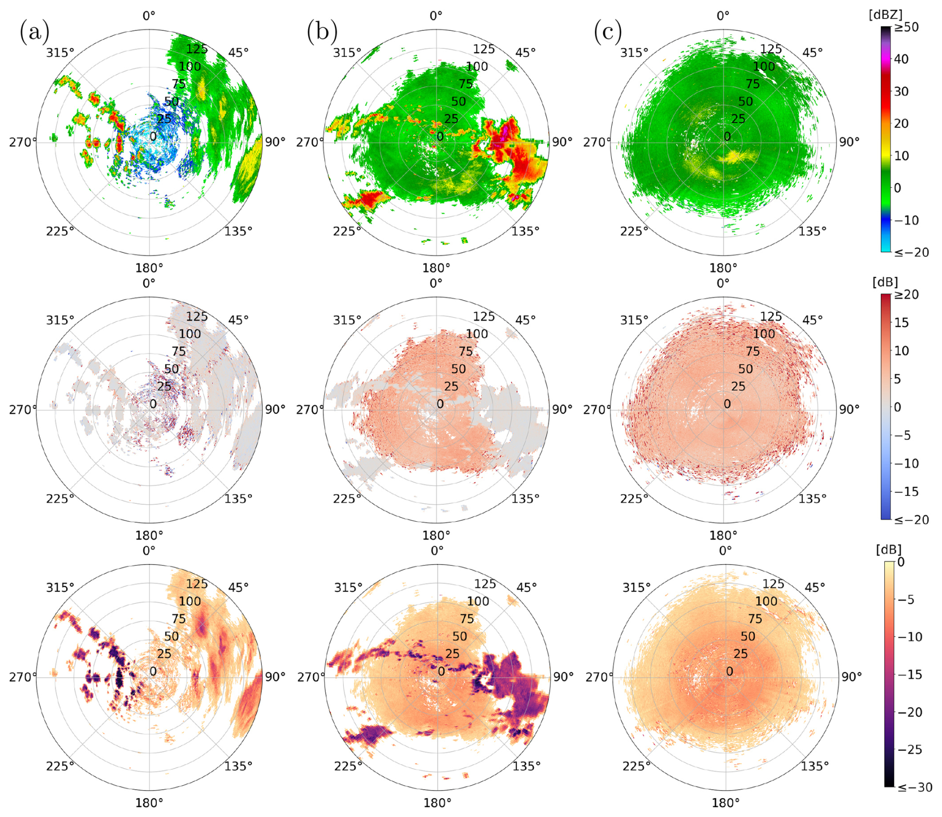
Figure 1 Horizontal reflectivity (first row), differential reflectivity (second row), and depolarization ratio (third row) for examples of (a) a winter sweep, (b) a mixed summer sweep, and (c) a cluttered summer sweep. White pixels are filtered by the initial preprocessing done by DWD. The sweeps shown were measured (a) on 9 January 2025, at 17:55 UTC in Flechtdorf, (b) on 16 June 2022, at 09:00 UTC in Dresden and (c) on 18 June 2022, at 10:00 UTC in Isen.

The DWD provided all terrain-following sweeps measured at the 17 different dual-polarization weather radars for three one-hour time periods: 09:00–10:00 UTC on 16 June 2022, 10:00–11:00 UTC on 18 June 2022, and 17:00–18:00 UTC on 9 January 2025. Radar sweeps collected in January 2025 are referred to as winter sweeps, and radar sweeps collected in June 2022 are referred to as summer sweeps. Moreover, the radar sweeps collected on 16 June feature both meteorological and non-meteorological echoes and are referred to as mixed summer sweeps. In contrast, the radar sweeps collected on 18 June were collected during a time period when no precipitation was measured, indicating that only non-meteorological echoes were detected. Therefore, these sweeps are referred to as cluttered summer sweeps. For the winter sweeps, the specific time frame was chosen with the goal of selecting sweeps featuring a minimum amount of non-meteorological echoes. However, even for the winter sweeps, a certain amount of non-meteorological echoes cannot be avoided. Figure 1 shows examples of the radar moments DBZH, ZDR and UDR obtained from different sweeps measured during these time periods.

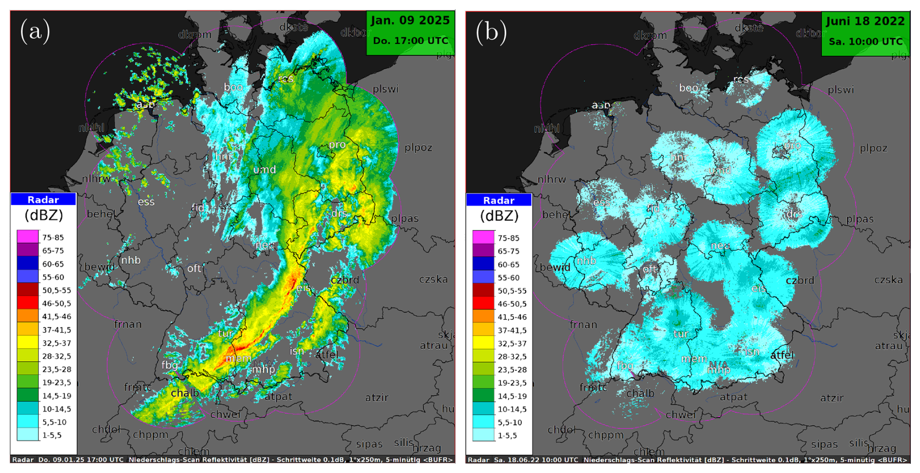
Figure 2 Composite radar images of the horizontal reflectivity over Germany: (a) the precipitation during the winter period, on 9 January 2025, at 17:00 UTC, and (b) the non-meteorological echoes during the cluttered summer period, on 18 June 2022, at 10:00 UTC.

The winter sweeps contain a variety of precipitation features (Fig. 2a), with isolated showers over north-western Germany, widespread stratiform precipitation in north-eastern Germany, a convective line over southern Germany, and some very light precipitation similar to insect signatures. The cluttered summer sweeps show different insect signatures for different radars (Fig. 2b): the radars in the south and east of Germany show strong insect signatures, whereas the radars in the north and north-west show lighter signatures.

2.2 Preprocessing of radar data

For each radar station, a single sweep consists of the measured values of the radar moments at the radar gates covered by the radar. These radar gates partition the scanned area into a polar grid defined by the radar's number of rays $n_{\mathrm{a}}\in \mathbb{N}=\mathit{\{}\mathrm{1},\mathrm{2},\mathrm{\dots }\mathit{\}}$ and the number of range bins n_r∈ℕ. More specifically, the radar gate corresponding to the ith range bin of the jth ray is defined as the set

$$\begin{array}{}\text{(1)}& g_{i,j}=\mathit{\{}wr\left(\begin{array}{c}\sin \mathit{\alpha }\\ \cos \mathit{\alpha }\end{array}\right):r\in (i-\mathrm{1},i],\mathit{\alpha }\in ({\displaystyle \frac{\mathrm{2}\mathit{\pi }}{n_{\mathrm{a}}}}(j-\mathrm{1}),{\displaystyle \frac{\mathrm{2}\mathit{\pi }}{n_{\mathrm{a}}}}j\left]\mathit{\right\}}\subset {\mathbb{R}}^{\mathrm{2}},\end{array}$$

where w=250 denotes the range resolution of the radar in meters, r is the distance from the radar site in units of the range resolution w, and the azimuthal angle α is measured clockwise from north.

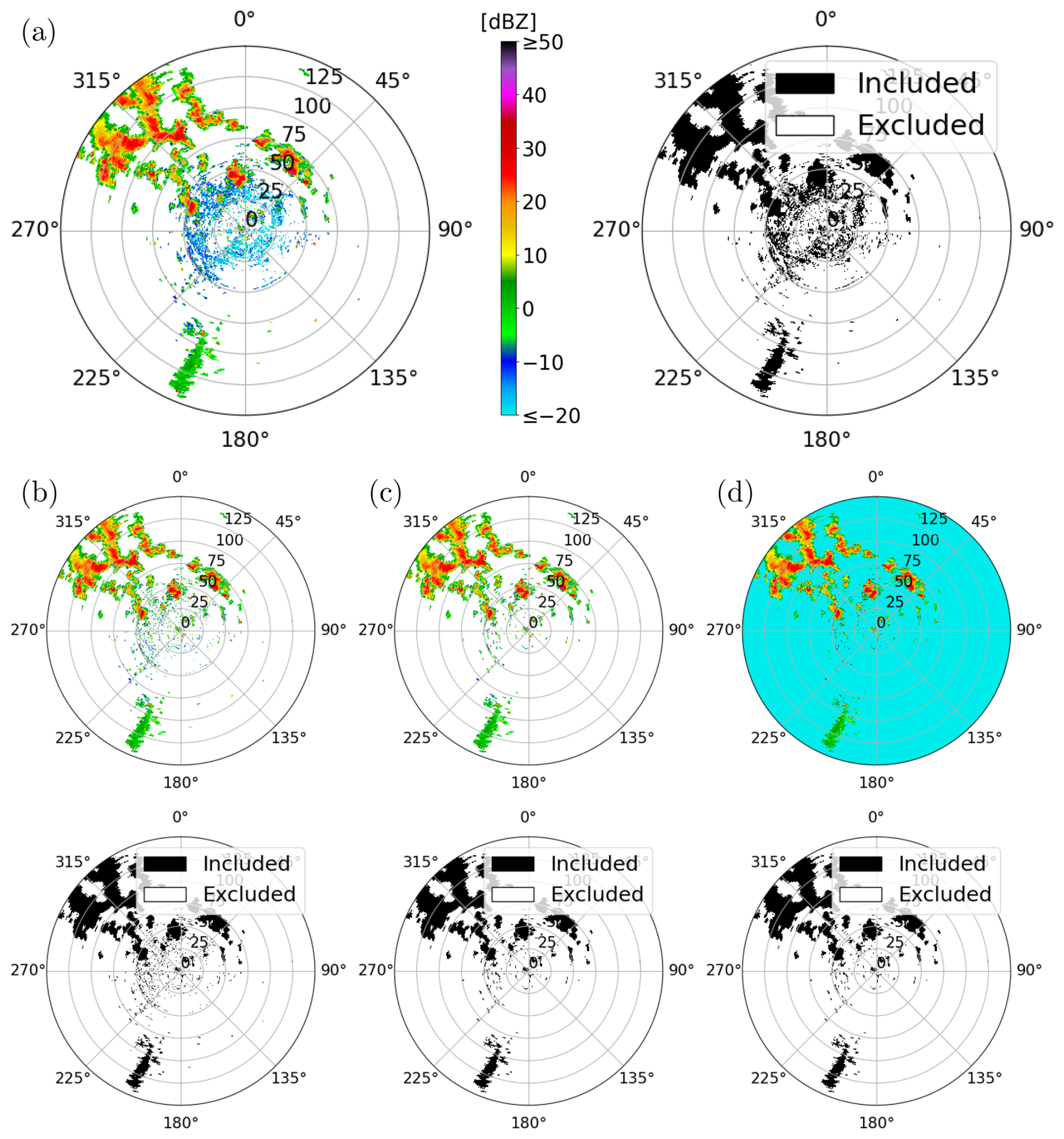
Figure 3 Cartesian representations of DBZH images: (a) DBZH image measured in winter, as provided by DWD, (b) after thresholding, (c) after despeckling, and (d) final DBZH image with placeholder values. White pixels in the DBZH images are either filtered out during the preprocessing by DWD or are assigned a placeholder value. The radar image shown was measured on 9 January 2025, at 17:00 UTC in Essen.

Let ℳ denote the set of radar moments available for a given sweep. Then, for each radar moment m∈ℳ, its measured values from the sweep can be represented by a single-channel image $A^m=\left(A_{i,j}^m\right)\in {\mathbb{R}}^{n_{\mathrm{r}}\times n_{\mathrm{a}}}$. For each pixel $(i,j)\in \mathrm{\Omega }=\mathit{\{}\mathrm{1},\mathrm{\dots },n_{\mathrm{r}}\mathit{\}}\times \mathit{\{}\mathrm{1},\mathrm{\dots },n_{\mathrm{a}}\mathit{\}}$, the entry $A_{i,j}^m$ corresponds to the value of the radar moment m at the associated radar gate g_i,j. Single-channel images can be combined into a multi-channel image $A=(A^m{)}_{m\in {\mathcal{M}}^{\prime }}\in {\mathbb{R}}^{C\times n_{\mathrm{r}}\times n_{\mathrm{a}}}$, where ${\mathcal{M}}^{\prime }\subseteq \mathcal{M}$ is the subset of included radar moments and $C=\left|{\mathcal{M}}^{\prime }\right|$ is the number of channels. In the following, we refer to these multi-channel images as radar images. Moreover, the provided data also contains information on which radar gates had already been identified as non-meteorological during the preprocessing performed by DWD. For these radar gates, the corresponding pixels of the DBZH image are assigned a placeholder value $p=-\mathrm{40}\mathrm{dBZ}$, which lies far below the reflectivity range of meteorological echoes. Pixels with a horizontal reflectivity value of −40 dBZ are referred to as excluded pixels, as they conclusively do not correspond to meteorological echoes. All other pixels are referred to as included pixels. A Cartesian representation of a DBZH image is shown in Fig. 3a. Most of the radar images still contain pixels that likely correspond to non-meteorological echoes, even for radar images measured in winter. To filter some of these pixels out, we apply further preprocessing steps.

For example, as depicted in Fig. 3a, the DBZH images show weak signals with horizontal reflectivity values below −10 dBZ near the radar. However, only very light drizzle could produce reflectivity values of that magnitude. That is, thresholding at −10 dBZ most likely removes noise and clutter, and does not remove any convectively significant weather. Therefore, pixels with lower horizontal reflectivity values are considered to correspond to non-meteorological echoes and are thus excluded as potential meteorological echoes (Fig. 3b). Their DBZH values are then also set to −40 dBZ to mark them as excluded pixels.

Moreover, meteorological echoes observed in the radar images typically form connected components consisting of several pixels (Fig. 1). In contrast, isolated included pixels are assumed to correspond to non-meteorological echoes. For this reason, each DBZH image is further processed by a despeckle filter consisting of two steps. First, we use the Hoshen-Kopelman algorithm (Hoshen and Kopelman, 1976) to identify all connected components of included pixels. More specifically, we apply the algorithm to the binarized image obtained by thresholding at −40 dBZ, separating the excluded pixels from the included ones. Here, we use the 4-neighborhood, which means that two pixels $(i_{\mathrm{1}},j_{\mathrm{1}}),(i_{\mathrm{2}},j_{\mathrm{2}})\in \mathrm{\Omega }$ with $(i_{\mathrm{1}},j_{\mathrm{1}})\ne (i_{\mathrm{2}},j_{\mathrm{2}})$ are neighboring if their associated radar gates $g_{i_{\mathrm{1}},j_{\mathrm{1}}},g_{i_{\mathrm{2}},j_{\mathrm{2}}}$ share a common edge. Note that the DBZH image is periodic in the second component, see Eq. (1), since each index $j\in \mathit{\{}\mathrm{1},\mathrm{\dots },n_{\mathrm{a}}\mathit{\}}$ represents the azimuthal angle of a ray, and the image corresponds to a sweep. Consequently, pixels corresponding to the first and last ray are neighboring if they have the same range index $i\in \mathit{\{}\mathrm{1},\mathrm{\dots },n_{\mathrm{r}}\mathit{\}}$. More precisely, for each pixel $(i,j)\in \mathrm{\Omega }$, the set $N_{(i,j)}\subset \mathrm{\Omega }$ of neighboring pixels can be written as $N_{(i,j)}=\left\{(k,\mathrm{\ell })\in \mathrm{\Omega }:|i-k|+d(j,\mathrm{\ell })=\mathrm{1}\right\}$, where $d:\mathit{\{}\mathrm{1},\mathrm{\dots },n_{\mathrm{a}}\mathit{\}}\times \mathit{\{}\mathrm{1},\mathrm{\dots },n_{\mathrm{a}}\mathit{\}}\to {\mathbb{N}}_{\mathrm{0}}$ denotes the periodic distance measure, given by

$$\begin{array}{}\text{(2)}& d(j,\mathrm{\ell })=min\mathit{\left\{}\right|j-\mathrm{\ell }|,n_{\mathrm{a}}-|j-\mathrm{\ell }\left|\mathit{\right\}}.\end{array}$$

for each $\mathrm{\ell }\in \mathit{\{}\mathrm{1},\mathrm{\dots },n_{\mathrm{a}}\mathit{\}}$. After identifying the connected components, those consisting of less than six undetermined pixels are selected. Then, the DBZH values of pixels $(i,j)\in \mathrm{\Omega }$ in these components are set to −40 dBZ, indicating that they do not correspond to meteorological echoes. The result of the despeckling process is shown in Fig. 3c.

For the excluded pixels $(i,j)\in \mathrm{\Omega }$, their corresponding entries in the DBZH image were set to −40 dBZ to indicate that they conclusively do not correspond to meteorological echoes (Fig. 3d). For the other radar moments, ZDR and UDR, we also assign specific placeholder values p∈ℝ to the entries of their single-channel images. Similar to the horizontal reflectivity, these placeholder values are chosen to lie outside the range of typical values for meteorological echoes in our dataset. More specifically, for the differential reflectivity, the placeholder value is set to p=20 dB. This particular value was chosen since it lies above typical values for meteorological echoes (around 0 dB), but within the range for non-meteorological echoes (between 5 and 20 dB) in our data, as can be seen in Fig. 1b and c. Furthermore, as described in Kilambi et al. (2018), except for some special cases such as hail, the depolarization ratio of meteorological scatterers is typically below −12 dB. In contrast, the depolarization ratio of non-meteorological scatterers typically ranges between −12 and 0 dB. Therefore, we chose a placeholder value of p=0 dB for the depolarization ratio.

The presented preprocessing steps remove most of the clutter with low reflectivity values. However, many mixed summer radar images contain much larger connected components corresponding to more reflective non-meteorological scatterers, as can be seen in Fig. 1b. Detecting such echoes presents a challenging task for conventional methods such as fuzzy logic filtering (Dufton and Collier, 2015) or depolarization ratio thresholding (Kilambi et al., 2018).

2.3 Description of the network architecture

The task of detecting non-meteorological echoes can be viewed as a segmentation task of multi-channel two-dimensional (2D) radar image data. Each pixel of the image is classified as corresponding to meteorological or non-meteorological echoes, that is, each pixel is assigned a binary class label $c\in \mathit{\{}\mathrm{0},\mathrm{1}\mathit{\}}$. In Ronneberger et al. (2015), the so-called U-net architecture, a fully convolutional neural network, has been introduced to address similar segmentation tasks of 2D images.

A U-net has an encoder-decoder architecture with skip connections, consisting of a so-called contracting path that downsamples the spatial resolution of the features and an expansive path that upsamples it again. Both the downsampling and the upsampling paths consist of several levels. The network considered in the present paper is an adapted version of the U-net architecture comprising five levels, with the fifth level acting as a bottleneck. Consequently, the network performs four downsampling steps and four upsampling steps. Each downsampling step consists of two convolution blocks and a 2×2 max-pooling layer for downsampling the spatial resolution of the feature map (Goodfellow et al., 2016). A convolution block contains a padded 3×3 convolutional layer, followed by a batch normalization layer and a rectified linear unit (ReLU) activation function, which is given by $\mathrm{ReLU}:\mathbb{R}\to {\mathbb{R}}_{\mathrm{0}}^{+}=[\mathrm{0},\mathrm{\infty })$, $\mathrm{ReLU}\left(x\right)=max(x,\mathrm{0})$. The convolution blocks of the first downsampling step produce n_f∈ℕ feature channels, and each further downsampling step doubles the number of feature channels. The bottleneck at the fifth layer consists of two such convolution blocks. For each of the subsequent upsampling steps, the spatial resolution of the feature channels is increased using bilinear interpolation (Dumitrescu and Boiangiu, 2019). The resulting channels are then concatenated with the feature channels of the corresponding level of the downsampling path. Two convolutional blocks following the concatenation of those feature channels divide the number of feature channels by three and complete the upsampling step. Here, the number of feature channels is divided by three since the concatenated channels consist of the channels of the downsampling path and twice as many interpolated channels from the level below. After the final upsampling step, the sigmoid activation function $\mathit{\sigma }:\mathbb{R}\to [\mathrm{0},\mathrm{1}]$, given by

$$\mathit{\sigma }\left(x\right)={\displaystyle \frac{\mathrm{1}}{\mathrm{1}+e^{-x}}},$$

is applied to the output.

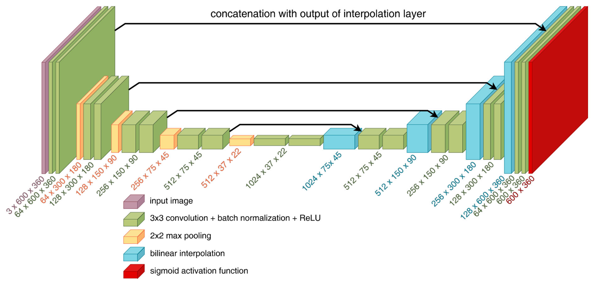
Figure 4 Schematic representation of the network architecture with n_f=64 feature channels in the first downsampling step. Below each layer, the respective output dimensions are given.

Compared to the original U-net architecture presented in Ronneberger et al. (2015), we use padded convolutional layers with a padding of 1 in each step, preserving the image size throughout the network. Since the network input is periodic in the second component, we use periodic padding (Schubert et al., 2019) in this direction, while the padding in the direction of the first component is reflective. Moreover, the spatial resolution of the features is upsampled using bilinear interpolation instead of an up-convolution. Furthermore, the network does not include a final 1×1 convolution. Instead, the output of the final convolution block is already a single-channel map to which the sigmoid activation function is applied directly. A sketch of the network architecture described above is shown in Fig. 4.

The network outputs are images of the same spatial dimensions as each of the input channels. More specifically, the network architecture stated above with parameter constellation $\mathit{\theta }\in \mathrm{\Theta }\subset {\mathbb{R}}^q$ is given by a function $f_{\mathit{\theta }}:{\mathbb{R}}^{k\times h\times w}\to [\mathrm{0},\mathrm{1}{]}^{h\times w}$, with spatial dimensions $h,w\in \mathbb{N}$ and the number of input channels k=3. Here, θ denotes the vector of trainable parameters of the network, and Θ⊂ℝ^q is the network's parameter space for some q∈ℕ depending on the number of feature channels n_f. Each input channel corresponds to a single-channel image of a radar moment, as described in Sect. 2.1, allowing the network to combine information about different radar moments to detect non-meteorological echoes.

The goal is then to perform supervised training of the network to assign binary labels to each pixel $(i,j)\in \mathrm{\Omega }$, describing which pixels correspond to meteorological and non-meteorological echoes, respectively. This training process requires pixel-wise labeled training data, that is, each pixel $(i,j)\in \mathrm{\Omega }$ must be assigned a ground truth class label $c_{i,j}\in \mathit{\{}\mathrm{0},\mathrm{1}\mathit{\}}$. However, mixed radar images containing both meteorological and non-meteorological echoes lack pixel-wise ground truth labels, and generating such labels by hand is very costly. Therefore, we propose a method to generate synthetic multi-channel images and corresponding pixel-wise ground truth labels for training the network.

2.4 Generation of synthetic training data

As outlined in Sect. 2.3, the network architecture considered in this paper can utilize radar images as input, where each channel corresponds to a single-channel image of a specific radar moment. The training samples consist of such radar images and corresponding binary ground truth images indicating whether each pixel corresponds to a meteorological or a non-meteorological echo. We generate synthetic radar images by combining radar images corresponding to winter sweeps (featuring meteorological echoes) and radar images corresponding to cluttered summer sweeps (featuring non-meteorological echoes). For brevity, we refer to these as winter radar images and cluttered summer radar images, respectively. This approach is motivated by the observation that the horizontal reflectivity (DBZH) values in mixed summer radar images often have the appearance of a combination of (scaled) DBZH values from winter and from cluttered summer radar images, as illustrated in Fig. 1b. In this way, we can generate labeled training samples where the contributions of meteorological and non-meteorological echoes are explicitly known, addressing the challenge of difficult labeling in mixed radar images. However, the meteorological echoes in the synthetic radar images are exclusively those of the winter radar images. Consequently, precipitation structures that occur in summer only are not represented in the training data.

More specifically, we generate a realistic mixed (synthetic) DBZH image by combining two DBZH images $A^{\mathrm{H},\mathrm{w}},A^{\mathrm{H},\mathrm{s}}\in {\mathbb{R}}^{n_{\mathrm{r}}\times n_{\mathrm{a}}}$ from a winter and a cluttered summer radar image, respectively, in the following manner. Since the horizontal reflectivity is measured in decibels, which is a logarithmic unit of measurement, we first transform the entries of the DBZH images into linear scale using the transformation $\mathrm{\Phi }:\mathbb{R}\to {\mathbb{R}}^{+}=(\mathrm{0},\mathrm{\infty })$ (Ryzhkov and Zrnić, 2019), which is given by

$$\mathrm{\Phi }\left(x\right)={\mathrm{10}}^{x/\mathrm{10}}.$$

The transformed reflectivity values are scaled by suitable weighting factors λ_w>0 and λ_s>0 for the DBZH images from the winter and the cluttered summer radar image, respectively. For each pixel, the scaled reflectivity values are summed up and transformed back into decibels to obtain the synthetic DBZH image $A^{\mathrm{H},\mathrm{m}}\in {\mathbb{R}}^{n_{\mathrm{r}}\times n_{\mathrm{a}}}$ with entries

$$A_{i,j}^{\mathrm{H},\mathrm{m}}=\left\{\begin{array}{ll}{\mathrm{\Phi }}^{-\mathrm{1}}\left({\mathit{\lambda }}_{\mathrm{w}}\mathrm{\Phi }\right(A_{i,j}^{\mathrm{H},\mathrm{w}})+{\mathit{\lambda }}_{\mathrm{s}}\mathrm{\Phi }(A_{i,j}^{\mathrm{H},\mathrm{s}}\left)\right),& \text{if }{A}_{i,j}^{\mathrm{H},\mathrm{w}}>-\mathrm{40}\mathrm{dBZ}\text{ or }\\ & A_{i,j}^{\mathrm{H},\mathrm{s}}>-\mathrm{40}\mathrm{dBZ},\\ -\mathrm{40},& \text{otherwise},\end{array}\right.$$

for each $(i,j)\in \mathrm{\Omega }$.

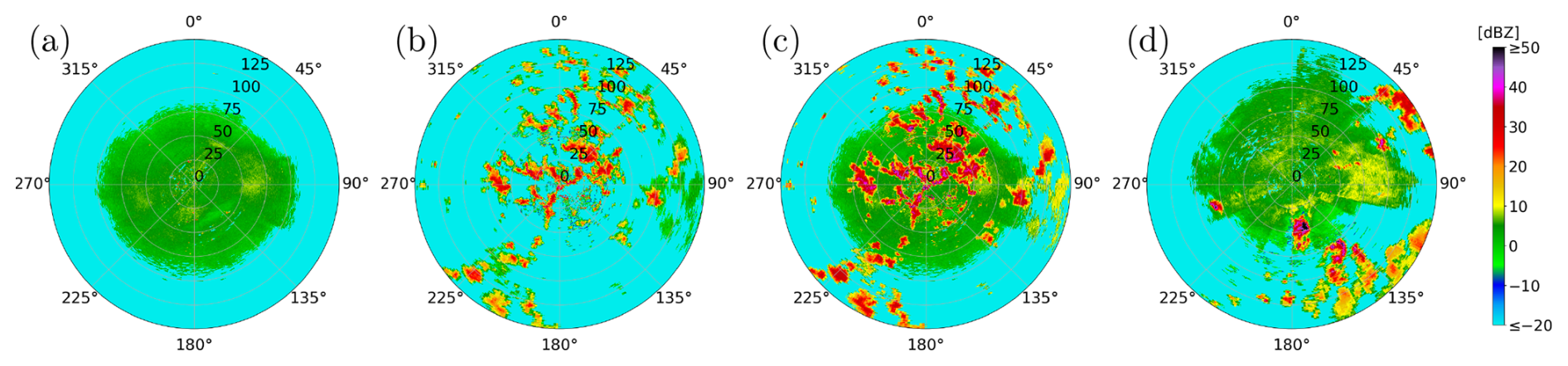
Figure 5 Comparison of Cartesian representations of different DBZH images: (a) cluttered summer radar image, (b) winter radar image, (c) their corresponding synthetic radar image with weighting factors λ_w=6.5, and λ_s=1 and (d) mixed summer radar image. The radar images shown were measured (a) on 18 June 2022, at 10:00 UTC in Neuheilenbach, (b) on 9 January 2025, at 17:00 UTC in Borkum and (d) on 16 June 2022, at 09:55 UTC in Memmingen.

Similarly to the placeholder values described in Sect. 2.2, we assign the entry of the synthetic DBZH image $A_{i,j}^{\mathrm{H},\mathrm{m}}$ a placeholder value $p=-\mathrm{40}\mathrm{dBZ}$ if the pixel is excluded for both radar images. To find appropriate weighting factors λ_w and λ_s, we consider the difference in horizontal reflectivity values observed in Fig. 1. Since the range of the horizontal reflectivity values corresponding to non-meteorological echoes is almost identical for cluttered summer radar images (Fig. 1c) and mixed summer radar images (Fig. 1b), the choice of λ_s=1 is suitable. However, the horizontal reflectivity values corresponding to meteorological echoes are substantially lower for winter radar images (Fig. 1a) compared to mixed summer radar images. Since the resulting synthetic DBZH image should resemble the typical DBZH images from mixed summer radar images, a weighting factor λ_w>1 is necessary. In order to determine a suitable choice, four representative mixed summer radar images were chosen. For each of them, a winter radar image with precipitation areas of similar size was assigned. Then, for different weighting factors ${\mathit{\lambda }}_{\mathrm{w}}\in \mathit{\{}\mathrm{1.5},\mathrm{3},\mathrm{5},\mathrm{8},\mathrm{15}\mathit{\}}$, we compared the DBZH values of manually sampled pixels within similar meteorological structures of both images. As a result, a weighting factor λ_w between 5 and 8 was deemed appropriate. Note that the weighting factors determined in this way are specific to the considered time periods, though the considered range for the weighting factor allows for calibration differences of up to 3 dB. Figure 5 shows how a synthetic DBZH image is generated by combining a winter and a cluttered summer radar image using a weighting factor λ_w=6.5. The resulting synthetic DBZH image (Fig. 5c) is then compared with one from a mixed summer radar image (Fig. 5d).

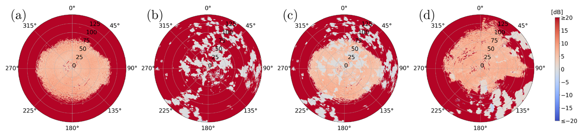
Figure 6 Comparison of Cartesian representations of different ZDR images: (a) cluttered summer radar image, (b) winter radar image, (c) their corresponding synthetic radar image, and (d) mixed summer radar image. The radar images shown were measured at the times and the radar stations mentioned in Fig. 5.

The two chosen winter and cluttered summer radar images are then also used to generate synthetic single-channel images for the other radar moments considered in Sect. 2.1. In addition to the horizontal reflectivity, which is proportional to the particle concentration and the particle's horizontal cross-section within the radar gate, the differential reflectivity (ZDR) primarily reflects the mean axis ratio of the particles (Straka et al., 2000). Since differential reflectivity is defined as the difference between horizontal and vertical reflectivity in decibels, synthetic values can be generated by taking the difference between synthetic horizontal and vertical reflectivity values. Similarly to the synthetic DBZH image A^H,m, a synthetic DBZV image $A^{\mathrm{V},\mathrm{m}}\in {\mathbb{R}}^{n_{\mathrm{r}}\times n_{\mathrm{a}}}$ is also generated. Then, the corresponding synthetic ZDR image is denoted by $A^{\mathrm{ZDR},\mathrm{m}}\in {\mathbb{R}}^{n_{\mathrm{r}}\times n_{\mathrm{a}}}$, and its entries are given by

$$A_{i,j}^{\mathrm{ZDR},\mathrm{m}}=\left\{\begin{array}{ll}{A}_{i,j}^{\mathrm{H},\mathrm{m}}-A_{i,j}^{\mathrm{V},\mathrm{m}},& \text{if }{A}_{i,j}^{\mathrm{H},\mathrm{m}}>-\mathrm{40}\\ & \text{ and }{A}_{i,j}^{\mathrm{V},\mathrm{m}}>-\mathrm{40},\\ \mathrm{20},& \text{if }{A}_{i,j}^{\mathrm{H},\mathrm{m}}=-\mathrm{40}\\ & \text{ or }{A}_{i,j}^{\mathrm{V},\mathrm{m}}=-\mathrm{40},\end{array}\right.$$

for each $(i,j)\in \mathrm{\Omega }$, see Fig. 6. Following Sect. 2.2, a placeholder value of p=20 dB is assigned to all entries of the synthetic ZDR image for which at least one of the corresponding synthetic DBZH and DBZV values is a placeholder value.

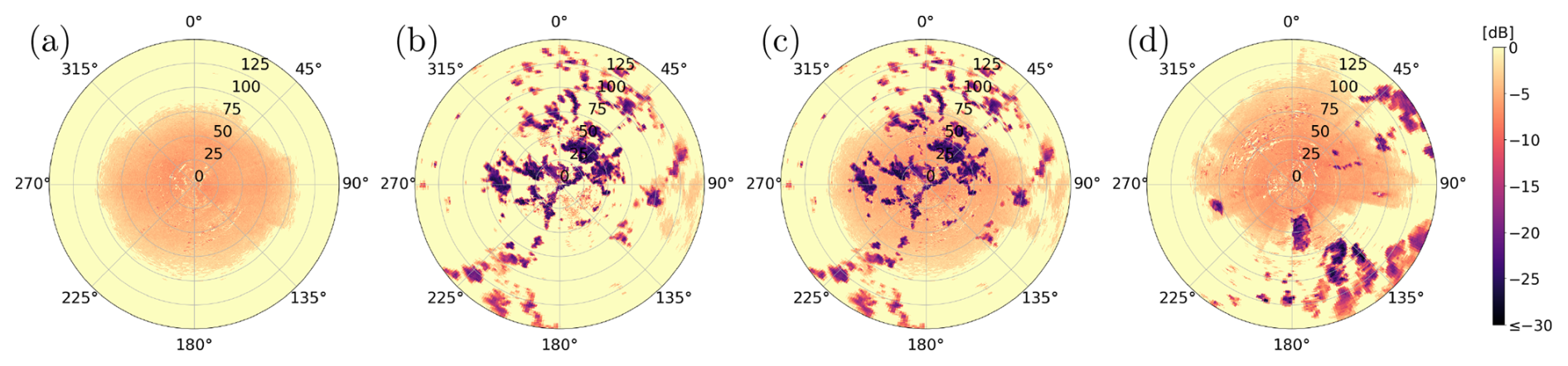
Figure 7 Comparison of Cartesian representations of different UDR images: (a) cluttered summer radar image, (b) winter radar image, (c) their corresponding synthetic radar image, and (d) mixed summer radar image. The radar images shown were measured at the times and the radar stations mentioned in Fig. 5.

In addition to describing the size and shape of particles using DBZH and ZDR, we also use the depolarization ratio UDR to quantify the homogeneity of the detected particles' shapes within a radar gate. To generate a synthetic UDR image $A^{\mathrm{UDR},\mathrm{m}}\in (-\mathrm{\infty },\mathrm{0}{]}^{n_{\mathrm{r}}\times n_{\mathrm{a}}}$, we use the property that pixels $(i,j)\in \mathrm{\Omega }$ included in the winter radar image are assumed to correspond to meteorological echoes. The corresponding entries from the synthetic UDR image are assigned the depolarization ratio values $A^{\mathrm{UDR},\mathrm{w}}\in (-\mathrm{\infty },\mathrm{0}{]}^{n_{\mathrm{r}}\times n_{\mathrm{a}}}$ from the winter radar image. Pixels excluded from the winter radar image are assigned the values $A^{\mathrm{UDR},\mathrm{s}}\in (-\mathrm{\infty },\mathrm{0}{]}^{n_{\mathrm{r}}\times n_{\mathrm{a}}}$ from the cluttered summer radar image if they are included in this radar image. Otherwise, they are assigned a placeholder value. More precisely, the entries of A^UDR,m are given by

$$A_{i,j}^{\mathrm{UDR},\mathrm{m}}=\left\{\begin{array}{ll}{A}_{i,j}^{\mathrm{UDR},\mathrm{w}},& \text{if }{A}^{\mathrm{H},\mathrm{w}}>-\mathrm{40}\mathrm{dBZ},\\ A_{i,j}^{\mathrm{UDR},\mathrm{s}},& \text{if }{A}^{\mathrm{H},\mathrm{w}}=-\mathrm{40}\mathrm{dBZ}\\ & \text{ and }{A}^{\mathrm{H},\mathrm{s}}>-\mathrm{40}\mathrm{dBZ},\\ \mathrm{0},& \text{otherwise},\end{array}\right.$$

for each $(i,j)\in \mathrm{\Omega }$, see Fig. 7. For pixels included in both radar images, the synthetic DBZH value combines both DBZH values. However, the synthetic UDR value for these pixels is taken from the winter radar image alone, since there is no physically obvious way of combining the two depolarization ratios.

Alongside the synthetic radar image $A^{\mathrm{m}}=(A^{\mathrm{H},\mathrm{m}},A^{\mathrm{ZDR},\mathrm{m}},A^{\mathrm{UDR},\mathrm{m}})\in {\mathbb{R}}^{\mathrm{3}\times n_{\mathrm{r}}\times n_{\mathrm{a}}}$, we generate a corresponding ground truth image $G\in \mathit{\{}\mathrm{0},\mathrm{1}{\mathit{\}}}^{n_{\mathrm{r}}\times n_{\mathrm{a}}}$. Its values indicate which pixels of the synthetic radar image correspond to meteorological $(G_{i,j}=\mathrm{0})$ and non-meteorological echoes $(G_{i,j}=\mathrm{1})$, respectively. Pixels included in the winter radar image A^H,w are assumed to correspond to meteorological echoes, as described in Sect. 2.2. Since the synthetic image is generated in such a way that these pixels also correspond to meteorological echoes in the synthetic image, they are assigned a ground truth label of 0. In particular, pixels that are also included in the cluttered summer radar image, and whose synthetic reflectivity values therefore contain both a meteorological and a non-meteorological contribution, are labeled as meteorological. In this way, every pixel corresponding to meteorological echoes is labeled as such. All of the other pixels, i.e., those excluded from the winter radar image, are labeled 1. More precisely, for each pixel $(i,j)\in \mathrm{\Omega }$, the ground truth label G_i,j is given by

$$G_{i,j}=\left\{\begin{array}{ll}\mathrm{0},& \text{if }{A}^{\mathrm{H},\mathrm{w}}>-\mathrm{40}\mathrm{dBZ},\\ \mathrm{1},& \text{otherwise.}\end{array}\right.$$

Generating synthetic radar images in this way provides mixed radar images with pixel-wise ground truth labeling, assigning each pixel as either meteorological or non-meteorological echoes. This ground truth allows the three synthetic channels to serve as training samples for the neural network.

2.5 Network training

The available winter dataset ${\mathcal{D}}^{\mathrm{w}}=\mathit{\{}{A}_n^{\mathrm{w}}{\mathit{\}}}_{n=\mathrm{1}}^{\mathrm{180}}\subset D={\mathbb{R}}^{\mathrm{3}\times n_{\mathrm{r}}\times n_{\mathrm{a}}}$ consists of 180 radar images $A_n^{\mathrm{w}}=(A_n^{\mathrm{H},\mathrm{w}},A_n^{\mathrm{V},\mathrm{w}},A_n^{\mathrm{UDR},\mathrm{w}})$, where the radar moments present in the data are horizontal reflectivity, vertical reflectivity, and the depolarization ratio. Similarly, the available cluttered summer dataset is given by ${\mathcal{D}}^{\mathrm{s}}=\mathit{\{}{A}_n^{\mathrm{s}}{\mathit{\}}}_{n=\mathrm{1}}^{\mathrm{180}}\subset D$. We partition each of these datasets into two disjoint subsets. One subset of radar images is used for generating the training samples, while the other subset is reserved for generating the validation samples, which are used for model selection, see Sect. 2.6. For this purpose, we partition the index set $\mathcal{I}=\mathit{\{}\mathrm{1},\mathrm{\dots },\mathrm{180}\mathit{\}}$ into two disjoint subsets ${\mathcal{I}}_{\mathrm{train}},{\mathcal{I}}_{\mathrm{val}}\subset \mathcal{I}$, i.e.,

$${\mathcal{I}}_{\mathrm{train}}\cup {\mathcal{I}}_{\mathrm{val}}=\mathcal{I}\text{and}{\mathcal{I}}_{\mathrm{train}}\cap {\mathcal{I}}_{\mathrm{val}}=\mathrm{\varnothing }.$$

The index sets ${\mathcal{I}}_{\mathrm{train}},{\mathcal{I}}_{\mathrm{val}}\subset \mathcal{I}$ are chosen so that all winter and cluttered summer radar images from a single radar station (radar Essen) are used for the generation of validation samples, while the radar images from other radar stations are used for the generation of training samples.

We use the methodology described in Sect. 2.4 to generate synthetic training samples by combining radar images from the winter and cluttered summer datasets. Each synthetic training sample consists of a synthetic radar image A∈D and a corresponding ground truth image $G\in \mathit{\{}\mathrm{0},\mathrm{1}{\mathit{\}}}^{n_{\mathrm{r}}\times n_{\mathrm{a}}}$. The synthetic radar image comprises the radar moments of horizontal reflectivity, differential reflectivity, and the depolarization ratio, i.e., $A=(A^{\mathrm{H}},A^{\mathrm{ZDR}},A^{\mathrm{UDR}})$. Before generating the synthetic training samples, we apply various data augmentation steps to increase their diversity. More precisely, as described in Sect. 2.4, the DBZH and DBZV images from the winter and cluttered summer datasets are scaled by reflectivity weighting factors ${\mathit{\lambda }}_{\mathrm{w}},{\mathit{\lambda }}_{\mathrm{s}}>\mathrm{0}$, respectively. In addition, we apply a rotation and a possible inversion of orientation.

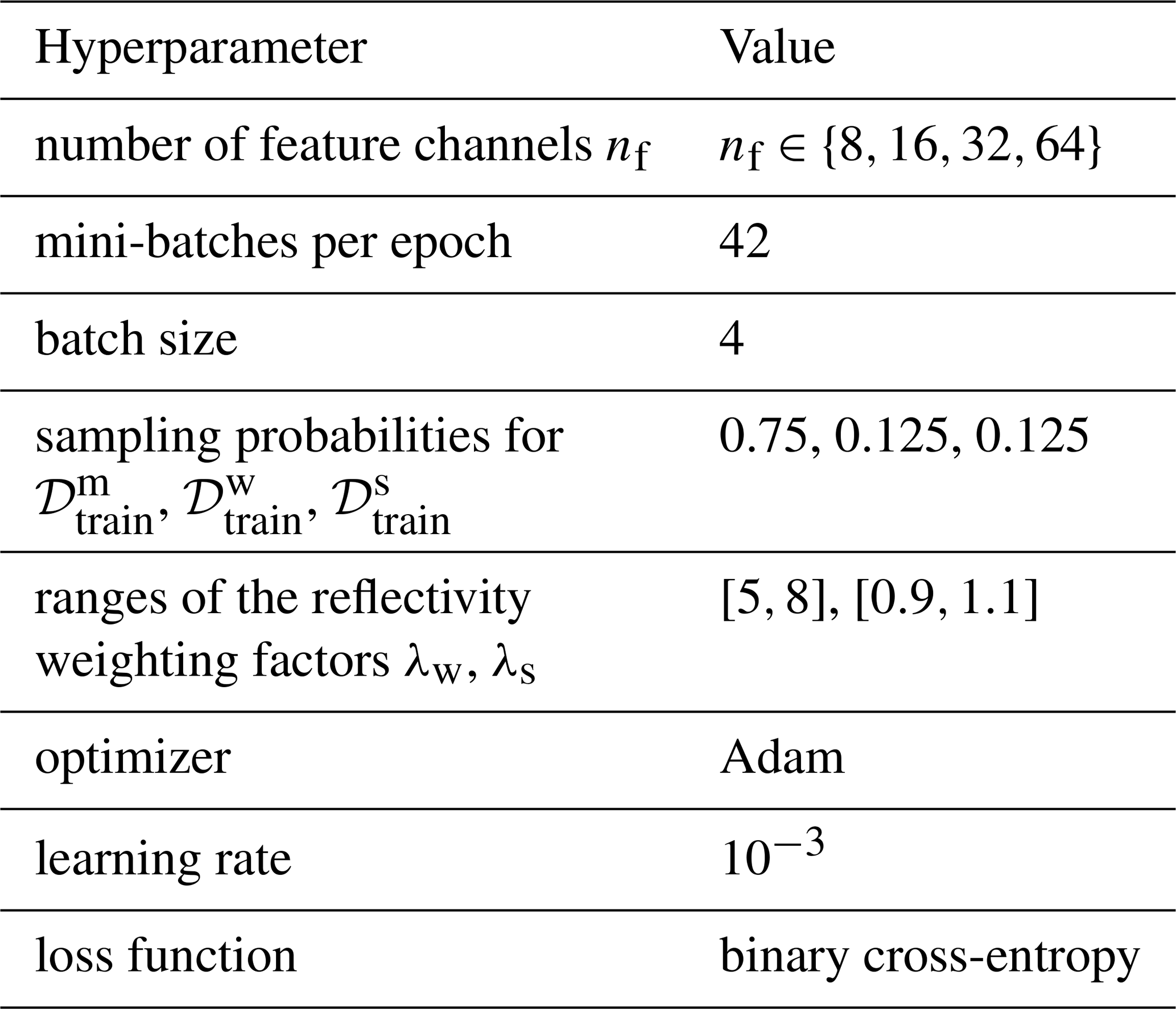
Specifically, we introduce a parametric mapping $g_{\mathit{\psi },{\mathit{\psi }}^{\prime }}:D\times D\to D\times \mathit{\{}\mathrm{0},\mathrm{1}{\mathit{\}}}^{n_{\mathrm{r}}\times n_{\mathrm{a}}}$ that combines two radar images to generate a synthetic radar image and a corresponding ground truth image. The space of admissible parameters for data augmentation is given by $\mathrm{\Psi }={\mathbb{R}}^{+}\times \mathit{\{}\mathrm{1},\mathrm{\dots },n_{\mathrm{a}}\mathit{\}}\times \mathit{\{}-\mathrm{1},\mathrm{1}\mathit{\}}$. Each parameter vector $\mathit{\psi }=(\mathit{\lambda },\mathit{\phi },o)\in \mathrm{\Psi }$ contains the reflectivity weighting factor λ>0, the rotation angle $\mathit{\phi }\in \mathit{\{}\mathrm{1},\mathrm{\dots },n_{\mathrm{a}}\mathit{\}}$, and the orientation flag $o\in \mathit{\{}-\mathrm{1},\mathrm{1}\mathit{\}}$. Here, a rotation angle of $\mathit{\phi }\in \mathit{\{}\mathrm{1},\mathrm{\dots },n_{\mathrm{a}}\mathit{\}}$ indicates a rotation by φ rays. Hence, a shift of φ rows is applied to the radar image. An orientation flag of $o=-\mathrm{1}$ indicates an inverted orientation. In that case, the radar image is flipped along the x-axis. To distinguish the transformations we apply to winter and cluttered summer radar images, we introduce restricted admissible parameter spaces ${\mathrm{\Psi }}^{\mathrm{w}},{\mathrm{\Psi }}^{\mathrm{s}}\subset \mathrm{\Psi }$. They only differ in the admissible range of the reflectivity weighting factor, which is given by the interval [5,8] for Ψ^w and by [0.9,1.1] for Ψ^s. The set of synthetic training samples generated by combining two radar images is then denoted by

$${\mathcal{D}}_{\mathrm{train}}^{\mathrm{m}}=\mathit{\left\{}{g}_{{\mathit{\psi }}_{\mathrm{w}},{\mathit{\psi }}_{\mathrm{s}}}\right(A_{n_{\mathrm{w}}}^{\mathrm{w}},A_{n_{\mathrm{s}}}^{\mathrm{s}}):{\mathit{\psi }}_{\mathrm{w}}\in {\mathrm{\Psi }}^{\mathrm{w}},{\mathit{\psi }}_{\mathrm{s}}\in {\mathrm{\Psi }}^{\mathrm{s}},n_{\mathrm{w}},n_{\mathrm{s}}\in {\mathcal{I}}_{\mathrm{train}}\mathit{\}}.$$

Note that, in order to make use of as many different combinations as possible, the indices $n_{\mathrm{w}},n_{\mathrm{s}}\in {\mathcal{I}}_{\mathrm{train}}$ of the winter and the cluttered summer radar image of a training sample are not matched by radar station or measurement time. In particular, radar images from different radar stations are combined for the generation of synthetic radar images.

These synthetic training samples feature both meteorological and non-meteorological echoes. However, in the training process, the network should be provided with training samples from various scenarios. Since the radar images from the winter and cluttered summer datasets, 𝒟^w and 𝒟^s, are used to represent meteorological and non-meteorological echoes, respectively, it is possible to generate synthetic radar images that feature only one type of echo. To this end, we introduce a radar image A^exc∈D in which all pixels are excluded, i.e., all of its entries are assigned the corresponding placeholder values. A synthetic radar image that features only meteorological echoes is then generated by combining a winter radar image and the radar image A^exc. In particular, the set of training samples featuring only meteorological echoes is given by

$${\mathcal{D}}_{\mathrm{train}}^{\mathrm{w}}=\mathit{\left\{}{g}_{{\mathit{\psi }}_{\mathrm{w}},\mathit{\psi }}\right(A_{n_{\mathrm{w}}}^{\mathrm{w}},A^{\mathrm{exc}}):{\mathit{\psi }}_{\mathrm{w}}\in {\mathrm{\Psi }}^{\mathrm{w}},\mathit{\psi }\in \mathrm{\Psi },n_{\mathrm{w}}\in {\mathcal{I}}_{\mathrm{train}}\mathit{\}}.$$

Analogously, the set of synthetic radar images featuring only non-meteorological echoes is given by

$${\mathcal{D}}_{\mathrm{train}}^{\mathrm{s}}=\mathit{\left\{}{g}_{\mathit{\psi },{\mathit{\psi }}_{\mathrm{s}}}\right(A^{\mathrm{exc}},A_{n_{\mathrm{s}}}^{\mathrm{s}}):\mathit{\psi }\in \mathrm{\Psi },{\mathit{\psi }}_{\mathrm{s}}\in {\mathrm{\Psi }}^{\mathrm{s}},n_{\mathrm{s}}\in {\mathcal{I}}_{\mathrm{train}}\mathit{\}}.$$

Note that the validation dataset ${\mathcal{D}}_{\mathrm{val}}^{\mathrm{m}}$, comprising radar images featuring both meteorological and non-meteorological echoes, and the validation datasets ${\mathcal{D}}_{\mathrm{val}}^{\mathrm{w}}$ and ${\mathcal{D}}_{\mathrm{val}}^{\mathrm{s}}$, comprising radar images featuring only one type of echo, are generated analogously using the index set ℐ_val instead of ℐ_train.

As stated in Sect. 2.3, the network can be described by its vector of trainable parameters θ∈Θ using a function $f_{\mathit{\theta }}:{\mathbb{R}}^{k\times h\times w}\to [\mathrm{0},\mathrm{1}{]}^{h\times w}$. Here, h=n_r and w=n_a denote the image dimensions of a single-channel image, and k=3 is the number of input channels. Then, for a given radar image A∈D, the output f_θ(A) of the network represents the matrix of probabilities (f_θ(A))_i,j that a pixel (i,j) corresponds to a non-meteorological echo for each $(i,j)\in \mathrm{\Omega }$.

The training process of the network involves iterating over so-called mini-batches, and the trainable parameters of the network are adapted at each iteration. More precisely, in each training step, a mini-batch $B=\mathit{\left\{}\right(A_n,G_n){\mathit{\}}}_{n=\mathrm{1}}^{\mathrm{4}}$ is built by generating a total of four synthetic radar images and corresponding ground truth images. Each training sample is chosen as follows: With a probability of 0.75, it is uniformly sampled from the training dataset ${\mathcal{D}}_{\mathrm{train}}^{\mathrm{m}}$ and therefore features both meteorological and non-meteorological echoes. Otherwise, we either sample it from ${\mathcal{D}}_{\mathrm{train}}^{\mathrm{w}}$ or ${\mathcal{D}}_{\mathrm{train}}^{\mathrm{s}}$, with a probability of 0.125 for each case. The mixed radar images are sampled most frequently since only they contain boundaries between meteorological and non-meteorological echoes, which are the most difficult regions to classify. The winter and cluttered summer samples ensure that the network also handles radar images featuring only one type of echo. For each training sample (A_n,G_n) of the mini-batch B, with $n\in \mathit{\{}\mathrm{1},\mathrm{2},\mathrm{3},\mathrm{4}\mathit{\}}$, the network output f_θ(A_n) is computed and compared to the ground truth image G_n using the binary cross-entropy loss, which is a measure of how well the network outputs match the ground truth images. More specifically, for any batch $B=\mathit{\left\{}\right(A_n,G_n){\mathit{\}}}_{n=\mathrm{1}}^{\mathrm{4}}$ and vector of trainable network parameters θ∈Θ, the cross-entropy loss L_θ(B) of the batch is given by

$$L_{\mathit{\theta }}\left(B\right)=-{\displaystyle \frac{\mathrm{1}}{\mathrm{4}}}\sum _{n=\mathrm{1}}^{\mathrm{4}}\sum _{(i,j)\in \mathrm{\Omega }}\mathrm{\ell }\left(f_{\mathit{\theta }}\right(A_n{)}_{i,j},\left(G_n{)}_{i,j}\right),$$

where $\mathrm{\ell }(y,x)=x\log \left(y\right)+(\mathrm{1}-x)\log (\mathrm{1}-y)$, with f_θ(A_n)_i,j and (G_n)_i,j denoting the entries of f_θ(A_n) and G_n, respectively. After computing the cross-entropy loss L_θ(B), its gradient is computed with respect to the vector of trainable network parameters θ. Based on that, this parameter vector θ is then adjusted using the Adam optimizer (Kingma and Ba, 2017) with a learning rate of 10⁻³. The network was implemented and trained using PyTorch 2.8.0 (Ansel et al., 2024). The batch size, the sampling probabilities, and the learning rate were fixed before training and are not subject to the model selection described in Sect. 2.6. An overview of the hyperparameters of the network is shown in Table 1.

Table 1 Hyperparameters of the neural network and its training.

2.6 Model selection and early stopping

The number n_f of feature channels, see Sect. 2.3, determines the number of trainable parameters of the network. If it is too small, the network cannot learn the features that distinguish meteorological from non-meteorological echoes; if it is too large, the network can overfit, i.e., it may adapt to details of the synthetic training data that do not carry over to measured radar images. Similarly, the network is expected to fit the training data more closely with each training step, which can also lead to overfitting. Since suitable values are difficult to determine a priori, the number n_f of feature channels and the length of training are selected based on the validation datasets described in Sect. 2.5. More precisely, a fixed validation set $V=\mathit{\left\{}\right(A_n^{\mathrm{val}},G_n^{\mathrm{val}}){\mathit{\}}}_{n=\mathrm{1}}^N\subset {\mathcal{D}}_{\mathrm{val}}^{\mathrm{m}}\cup {\mathcal{D}}_{\mathrm{val}}^{\mathrm{w}}\cup {\mathcal{D}}_{\mathrm{val}}^{\mathrm{s}}$ consisting of N=144 validation samples is generated once before the training process. The training samples are generated in each training step as described in Sect. 2.5. Then, for each $n_{\mathrm{f}}\in \mathit{\{}\mathrm{8},\mathrm{16},\mathrm{32},\mathrm{64}\mathit{\}}$, one network is trained as described above for up to 100 epochs consisting of 42 training steps each. For each $e\in \mathit{\{}\mathrm{1},\mathrm{\dots },\mathrm{100}\mathit{\}}$, its validation loss after e epochs is given by

$$L_{n_{\mathrm{f}},e}^{\mathrm{val}}=-{\displaystyle \frac{\mathrm{1}}{N}}\sum _{n=\mathrm{1}}^N\sum _{(i,j)\in \mathrm{\Omega }}\mathrm{\ell }\left(f_{{\mathit{\theta }}_{n_{\mathrm{f}},e}}\right(A_n^{\mathrm{val}}{)}_{i,j},\left(G_n^{\mathrm{val}}{)}_{i,j}\right),$$

where ${\mathit{\theta }}_{n_{\mathrm{f}},e}$ denotes the network's trainable parameters after e epochs. To prevent overfitting, the training is stopped early once the validation loss has not decreased over three consecutive intervals of five epochs, i.e., after the smallest epoch $e\in \mathit{\{}\mathrm{20},\mathrm{25},\mathrm{\dots },\mathrm{100}\mathit{\}}$ for which $L_{n_{\mathrm{f}},e-\mathrm{15}}^{\mathrm{val}}\le L_{n_{\mathrm{f}},e-\mathrm{10}}^{\mathrm{val}}\le L_{n_{\mathrm{f}},e-\mathrm{5}}^{\mathrm{val}}\le L_{n_{\mathrm{f}},e}^{\mathrm{val}}$. If there is no such epoch, the training ends after 100 epochs. The last epoch is denoted by $e_{n_{\mathrm{f}}}^{\mathrm{end}}$.

The number of feature channels and training epochs of the network are selected based on the moving average of the validation loss over the set $E_{n_{\mathrm{f}},e}=\mathit{\{}e-\mathrm{2},\mathrm{\dots },e+\mathrm{2}\mathit{\}}\cap \mathit{\{}\mathrm{1},\mathrm{\dots },e_{n_{\mathrm{f}}}^{\mathrm{end}}\mathit{\}}$ of up to five epochs surrounding $e\in \mathit{\{}\mathrm{1},\mathrm{\dots },e_{n_{\mathrm{f}}}^{\mathrm{end}}\mathit{\}}$, given by

$${\stackrel{\mathrm{‾}}{L}}_{n_{\mathrm{f}},e}^{\mathrm{val}}={\displaystyle \frac{\mathrm{1}}{\left|E_{n_{\mathrm{f}},e}\right|}}\sum _{k\in E_{n_{\mathrm{f}},e}}{L}_{n_{\mathrm{f}},k}^{\mathrm{val}}.$$

This moving average is considered in order to reduce the influence of fluctuations between single epochs, which can be quite large due to the small validation set. For the first two and the last two epochs, the set $E_{n_{\mathrm{f}},e}$ contains only three or four epochs, so that the last epochs are not excluded from the selection. Among all pairs (n_f,e) with $n_{\mathrm{f}}\in \mathit{\{}\mathrm{8},\mathrm{16},\mathrm{32},\mathrm{64}\mathit{\}}$ and $e\in \mathit{\{}\mathrm{1},\mathrm{\dots },e_{n_{\mathrm{f}}}^{\mathrm{end}}\mathit{\}}$, the selected number of feature channels $n_{\mathrm{f}}^{\ast }$ and the selected epoch e^∗ are then given by

$$(n_{\mathrm{f}}^{\ast },e^{\ast })=\begin{array}{ll}\mathrm{argmin}& {\stackrel{\mathrm{‾}}{L}}_{n_{\mathrm{f}},e}^{\mathrm{val}},\\ n_{\mathrm{f}}\in \mathit{\{}\mathrm{8},\mathrm{16},\mathrm{32},\mathrm{64}\mathit{\}}& \\ e\in \mathit{\{}\mathrm{1},\mathrm{\dots },e_{n_{\mathrm{f}}}^{\mathrm{end}}\mathit{\}}& \end{array}$$

and the trainable parameters of the selected network are denoted by ${\mathit{\theta }}^{\ast }={\mathit{\theta }}_{n_{\mathrm{f}}^{\ast },e^{\ast }}$.

2.7 Metrics for quantitative evaluation

To quantitatively evaluate the segmentation performance, we compare the network output against corresponding ground truth. For that purpose, pixels $(i,j)\in \mathrm{\Omega }$ with a horizontal reflectivity value of $A_{i,j}^{\mathrm{H}}=-\mathrm{40}\mathrm{dBZ}$ are excluded from the evaluation, as they conclusively do not correspond to meteorological echoes. Furthermore, the physical area of a radar gate g_i,j increases linearly with its distance from the radar. Therefore, to obtain metrics with a meaningful physical interpretation regarding the spatial extent of the echoes, we introduce a weight matrix $W=\left(W_{i,j}\right)\in {\mathbb{R}}^{n_{\mathrm{r}}\times n_{\mathrm{a}}}$. For each pixel $(i,j)\in \mathrm{\Omega }$, its weight W_i,j is given by

$$W_{i,j}=\left\{\begin{array}{ll}{a}_i,& \text{if }{A}_{i,j}^{\mathrm{H}}>-\mathrm{40}\mathrm{dBZ},\\ \mathrm{0},& \text{otherwise}.\end{array}\right.$$

Here, $a_i=\frac{\mathit{\pi }}{n_{\mathrm{a}}}(\mathrm{2}{r}_i-w)w$ denotes the physical area of radar gate g_i,j, where w=250 is the range resolution in meters, and r_i=iw is the outer radius of the radar gate. Using the weights of the individual pixels, we define the weighted area 𝒜(Ω^′) of any subset of pixels ${\mathrm{\Omega }}^{\prime }\subset \mathrm{\Omega }$ as the sum of the weights of the pixels in that set, given by

$$\mathcal{A}({\mathrm{\Omega }}^{\prime },W)=\sum _{(i,j)\in {\mathrm{\Omega }}^{\prime }}{W}_{i,j}.$$

Using a radar image $A\in D={\mathbb{R}}^{\mathrm{3}\times n_{\mathrm{r}}\times n_{\mathrm{a}}}$ as input, the network output $f_{{\mathit{\theta }}^{\ast }}\left(A\right)\in [\mathrm{0},\mathrm{1}{]}^{n_{\mathrm{r}}\times n_{\mathrm{a}}}$ is transformed into a binary prediction $P=\left(P_{i,j}\right)\in \mathit{\{}\mathrm{0},\mathrm{1}{\mathit{\}}}^{n_{\mathrm{r}}\times n_{\mathrm{a}}}$ by thresholding at 0.5. Specifically, the prediction P_i,j at pixel $(i,j)\in \mathrm{\Omega }$ is given by

$$P_{i,j}=\left\{\begin{array}{l}\mathrm{0},\text{if }\left(f_{{\mathit{\theta }}^{\ast }}\right(A){)}_{i,j}<\mathrm{0.5},\\ \mathrm{1},\text{if }\left(f_{{\mathit{\theta }}^{\ast }}\right(A){)}_{i,j}\ge \mathrm{0.5},\end{array}\right.$$

where prediction $P_{i,j}=\mathrm{0}$ represents meteorological echoes, and $P_{i,j}=\mathrm{1}$ represents non-meteorological echoes.

To quantify segmentation performance, we compute the area-weighted intersection over union (IOU), also referred to as the critical success index (Mbizvo and Larner, 2024). For class $c\in \mathit{\{}\mathrm{0},\mathrm{1}\mathit{\}}$, the class-specific IOU is defined as the ratio of the area of the intersection of pixels classified as class c in the prediction and pixels labeled as class c in the ground truth, to the area of their union, given by

$${\mathrm{IOU}}^c(G,P,W)={\displaystyle \frac{\mathcal{A}(\mathrm{\Omega }{|}_{P=c}\cap \mathrm{\Omega }{|}_{G=c},W)}{\mathcal{A}(\mathrm{\Omega }{|}_{P=c}\cup \mathrm{\Omega }{|}_{G=c},W)}}.$$

Here, the set of pixels assigned to class c by the prediction P and the set of pixels labeled as class c in the ground truth G are given by

$$\begin{array}{rl}& \mathrm{\Omega }{|}_{P=c}=\mathit{\left\{}\right(i,j)\in \mathrm{\Omega }:P_{i,j}=c\mathit{\}}\text{and}\\ & \mathrm{\Omega }{|}_{G=c}=\mathit{\left\{}\right(i,j)\in \mathrm{\Omega }:G_{i,j}=c\mathit{\}},\end{array}$$

respectively. We then obtain a single performance metric for the entire radar image by computing the combined IOU as the area-weighted sum of the class-specific IOUs, given by

$$\mathrm{IOU}(G,P,W)=\sum _{c\in \mathit{\{}\mathrm{0},\mathrm{1}\mathit{\}}}{\displaystyle \frac{\mathcal{A}\left(\mathrm{\Omega }{|}_{G=c}\right)}{\mathcal{A}\left(\mathrm{\Omega }\right)}}{\mathrm{IOU}}^c(G,P,W).$$

While the area-weighted IOU is an effective aggregate metric for overall segmentation quality, it does not distinguish between incorrectly classifying pixels as meteorological and incorrectly classifying pixels as non-meteorological echoes. Therefore, it is helpful to quantify the portion of correct predictions within specific regions, e.g., regions labeled as class c=0 in the ground truth. To this end, we define the area-weighted accuracy on a subset ${\mathrm{\Omega }}^{\prime }\subseteq \mathrm{\Omega }$. This metric calculates the portion of the weighted area within Ω^′ that is correctly classified and is given by

$$\mathrm{ACC}(G,P,W;{\mathrm{\Omega }}^{\prime })={\displaystyle \frac{\mathcal{A}({\mathrm{\Omega }}^{\prime }\cap \mathrm{\Omega }{|}_{P=G})}{\mathcal{A}\left({\mathrm{\Omega }}^{\prime }\right)}},$$

where $\mathrm{\Omega }{|}_{P=G}=\mathit{\left\{}\right(i,j)\in \mathrm{\Omega }:P_{i,j}=G_{i,j}\mathit{\}}$ denotes the set of all correctly classified pixels. Setting ${\mathrm{\Omega }}^{\prime }=\mathrm{\Omega }$ yields the area-weighted accuracy for the entire radar image.

This general formulation allows us to derive the class-specific precision and recall, which provide insight into specific error types. The precision PRE^c corresponds to the accuracy evaluated on $\mathrm{\Omega }{|}_{P=c}$, i.e., the set of pixels classified as class c. It quantifies the correctness of the prediction, where a low precision implies a high rate of false positives for class c, i.e., a large portion of pixels classified as class c are incorrectly classified. Conversely, the recall REC^c corresponds to the accuracy evaluated on $\mathrm{\Omega }{|}_{G=c}$, i.e., the set of pixels labeled as class c in the ground truth. It measures the completeness of the detection, where a low recall implies a high rate of false negatives, i.e., a large number of pixels with ground truth label c are incorrectly classified. These metrics are given by

$$\begin{array}{rl}& {\mathrm{PRE}}^c(G,P,W)=\mathrm{ACC}(G,P,W;\mathrm{\Omega }{|}_{P=c})\text{and}\\ & {\mathrm{REC}}^c(G,P,W)=\mathrm{ACC}(G,P,W;\mathrm{\Omega }{|}_{G=c}).\end{array}$$

While false positives for meteorological echoes (lower REC¹ and PRE⁰) introduce undesirable noise, missing weather events (lower REC⁰ and PRE¹) constitute a severe loss of information. From a meteorological perspective, a high recall REC⁰ for meteorological echoes is essential to ensure that weather events are correctly identified. This is particularly important for meteorological echoes with high reflectivity values, as they correspond to severe weather events. Therefore, we also investigate the network performance with respect to the horizontal reflectivity values A^H. For this, we evaluate the segmentation performance on subsets of pixels with horizontal reflectivity values $A_{i,j}^{\mathrm{H}}$ in the semi-open interval $[z,z+\mathrm{5})$ for $z\in \mathbb{R},$ given by

$$\mathrm{\Omega }{|}_{A^{\mathrm{H}}\in [z,z+\mathrm{5})}=\mathit{\left\{}\right(i,j)\in \mathrm{\Omega }:A_{i,j}^{\mathrm{H}}\in [z,z+\mathrm{5}\left)\mathit{\right\}}.$$

Similarly, we analyze the segmentation performance with respect to the distance from the radar, i.e., on subsets of pixels

$$\mathrm{\Omega }{|}_{i\in [r,r+\mathrm{19}]}=\mathit{\left\{}\right(i,j)\in \mathrm{\Omega }:r\le i\le r+\mathrm{19}\mathit{\}},$$

for range indices $r\in \mathit{\{}\mathrm{1},\mathrm{\dots },n_{\mathrm{r}}-\mathrm{19}\mathit{\}}$. This is motivated by the fact that non-meteorological echoes in winter radar images, which are rare but can appear close to the radar station, as shown in Fig. 3d, result in incorrect ground truth labels in the synthetically generated training data.

Using these subsets of pixels, we compute the area-weighted accuracy depending on reflectivity and distance from the radar, given by

$$\begin{array}{c}{\displaystyle }{\mathrm{ACC}}^{\text{H}}(G,P,W;z)=\mathrm{ACC}(G,P,W;\mathrm{\Omega }{|}_{A^{\mathrm{H}}\in [z,z+\mathrm{5})}),\\ {\displaystyle }{\mathrm{ACC}}^{\text{D}}(G,P,W;r)=\mathrm{ACC}(G,P,W;\mathrm{\Omega }{|}_{i\in [r,r+\mathrm{19}]}),\end{array}$$

respectively, and the recall for class $c\in \mathit{\{}\mathrm{0},\mathrm{1}\mathit{\}}$ depending on reflectivity and distance from the radar, given by

$$\begin{array}{c}{\displaystyle }{\mathrm{REC}}^{c,\text{H}}(G,P,W;z)=\mathrm{ACC}(G,P,W;\mathrm{\Omega }{|}_{G=c}\cap \mathrm{\Omega }{|}_{A^{\mathrm{H}}\in [z,z+\mathrm{5})}),\\ {\displaystyle }{\mathrm{REC}}^{c,\text{D}}(G,P,W;r)=\mathrm{ACC}(G,P,W;\mathrm{\Omega }{|}_{G=c}\cap \mathrm{\Omega }{|}_{i\in [r,r+\mathrm{19}]}),\end{array}$$

respectively.

Note that the introduced metrics can be computed for individual radar images and corresponding ground truth images, as well as for datasets $\mathcal{D}=\mathit{\left\{}\right(A_n,G_n){\mathit{\}}}_{n=\mathrm{1}}^N\subset D\times \mathit{\{}\mathrm{0},\mathrm{1}{\mathit{\}}}^{n_{\mathrm{r}}\times n_{\mathrm{a}}}$ consisting of N∈ℕ such image pairs. In this case, the metric is first computed for each radar image in the dataset individually and then aggregated as an area-weighted sum. For example, the area-weighted accuracy ACC on subsets ${\mathrm{\Omega }}^{\prime }=({\mathrm{\Omega }}_n^{\prime }{)}_{n=\mathrm{1}}^N\in {\mathrm{\Omega }}^N$ for the dataset 𝒟 is given by

$$\begin{array}{rl}\mathrm{ACC}& (\mathcal{D};{\mathrm{\Omega }}^{\prime })={\displaystyle \frac{\mathrm{1}}{{\sum }_{n=\mathrm{1}}^N\mathcal{A}({\mathrm{\Omega }}_n^{\prime },W_n)}}\sum _{n=\mathrm{1}}^N\mathcal{A}({\mathrm{\Omega }}_n^{\prime },W_n)\\ & \mathrm{ACC}(G_n,P_n,W_n;{\mathrm{\Omega }}_n^{\prime }),\end{array}$$

where $P_n\in \mathit{\{}\mathrm{0},\mathrm{1}{\mathit{\}}}^{n_{\mathrm{r}}\times n_{\mathrm{a}}}$ is the prediction and $W_n\in {\mathbb{R}}^{n_{\mathrm{r}}\times n_{\mathrm{a}}}$ is the weight matrix for the n-th radar image. As before, setting ${\mathrm{\Omega }}_n^{\prime }=\mathrm{\Omega }$ for all $n\in \mathit{\{}\mathrm{1},\mathrm{\dots },N\mathit{\}}$ yields the area-weighted accuracy for the dataset 𝒟, while the evaluation on ${\mathrm{\Omega }}_n^{\prime }=\mathrm{\Omega }{|}_{P_n=c}$ and ${\mathrm{\Omega }}_n^{\prime }=\mathrm{\Omega }{|}_{G_n=c}$ for all $n\in \mathit{\{}\mathrm{1},\mathrm{\dots },N\mathit{\}}$ and $c\in \mathit{\{}\mathrm{0},\mathrm{1}\mathit{\}}$ yields the class-specific precision and recall for the dataset 𝒟, respectively. Analogously, the intersection over union IOU for the dataset 𝒟 is given by

$$\mathrm{IOU}\left(\mathcal{D}\right)={\displaystyle \frac{\mathrm{1}}{{\sum }_{n=\mathrm{1}}^N\mathcal{A}(\mathrm{\Omega },W_n)}}\sum _{n=\mathrm{1}}^N\mathcal{A}(\mathrm{\Omega },W_n)\mathrm{IOU}(G_n,P_n,W_n).$$

3 State-of-the-art method

In this section, we describe the SotA method of DWD, which will be used as the benchmark for the evaluation in Sect. 4. It comprises a series of processing steps designed to identify and filter non-meteorological echoes, as well as a correction for attenuation, as described in Helmert et al. (2014). These processing steps include a threshold filter, a filter for spokes and rings, a blacklist filter, a polarimetric clutter filter based on fuzzy logic, a second-trip filter, and a speckle filter. Notably, the polarimetric clutter filter was extended in 2025 to include an additional so-called insect filter, which is used operationally during the summer months (April–October).

Echoes from insects, which are referred to as insect echoes, are typically characterized by the following features in the radar moments: reduced co-polar cross-correlation coefficient ρ_HV (<0.9), increased differential reflectivity ZDR (>2 dB), and low reflectivity factors DBZH and DBZV (<20 dBZ). In principle, most pixels corresponding to insect echoes can be correctly classified based on these features. However, there are also weather events, such as snowfall, that exhibit similar features, particularly at greater distances from the radar. Moreover, pixels corresponding to a mixture of meteorological echoes and clutter can also exhibit these features but should be classified as meteorological echoes.

The goal of the DWD insect filter is to filter out insect echoes, i.e., identify the corresponding pixels and classify them as non-meteorological echoes. It utilizes the radar moments introduced previously, as well as the so-called clutter correction moment (CCORH), which quantifies the portion of the reflectivity filtered out by the Doppler filter in dBZ. The insect filter is a decision tree-based pixel-wise classifier that considers radar moments and the statistical properties of the local neighborhood.

More precisely, the newly implemented insect filter operates in two steps: First, all pixels eligible for filtering are identified. Then, for each pixel identified in the first step, it is checked whether the pixel will be filtered based on UDR. In both steps, the so-called q×q neighborhood $N_{(i,j)}^{q\times q}\subset \mathrm{\Omega }$ of pixel $(i,j)\in \mathrm{\Omega }$ for an odd integer $q\in \mathit{\{}\mathrm{1},\mathrm{3},\mathrm{5},\mathrm{\dots }\mathit{\}}$ is used, which is given by

$$N_{(i,j)}^{q\times q}=\left\{(k,\mathrm{\ell })\in \mathrm{\Omega }:|i-k|\le {\displaystyle \frac{q-\mathrm{1}}{\mathrm{2}}}\text{ and }d(j,\mathrm{\ell })\le {\displaystyle \frac{q-\mathrm{1}}{\mathrm{2}}}\right\},$$

where d denotes the periodic distance measure as defined in Eq. (2). To incorporate information from the surroundings of a pixel into the filtering process, it has proven helpful to use percentile values. In contrast to using means, maxima, or minima, percentiles are insensitive to individual extreme values.

A pixel $(i,j)\in \mathrm{\Omega }$ is eligible for filtering if (a) its reflectivity value is below 20 dBZ, (b) the CCORH value in its 3×3 neighborhood $N_{(i,j)}^{\mathrm{3}\times \mathrm{3}}$ is not significant, and (c) the ZDR value in $N_{(i,j)}^{\mathrm{3}\times \mathrm{3}}$ is sufficiently different from 0 dB. All three conditions must be met simultaneously to prevent the misclassification of meteorological echoes. In particular, the CCORH condition was introduced to retain pixels within precipitation areas that, due to a mixture of meteorological echoes and clutter, exhibit a reduced quality of the polarimetric moments. Otherwise, they would be filtered out based on their high UDR value. Furthermore, the considered radar moments of snow and insects are very similar, except for ZDR. Therefore, the ZDR condition is necessary to retain pixels corresponding to weak snowfall, especially at greater distances from the radar.

To avoid filtering meteorological echoes at greater distances, where the reduced signal-to-noise ratio results in lower-quality polarimetric moments, an additional distance-dependent condition is implemented. Pixels at greater distances from the radar are only eligible for filtering if a certain percentage of pixels closer to the radar have already been filtered out by the insect filter. This condition accounts for the fact that insects usually occur in near-surface layers, and if insects are present at higher altitudes, they are typically also found closer to the ground.

An eligible pixel is filtered out if either the pixel itself has a high UDR value $(>-\mathrm{5}\mathrm{dB})$, or if high UDR values dominate in the local neighborhood (20th-percentile UDR in its 5×5 neighborhood $>-\mathrm{11}\mathrm{dB}$) and the pixel itself does not have a particularly low value ($<-\mathrm{18}\mathrm{dB}$). These two conditions ensure that pixels with a very high likelihood of non-meteorological echoes (based on their UDR values), as well as those mainly surrounded by pixels corresponding to non-meteorological echoes with moderate UDR values, are filtered out.

Note that the distance-dependent condition and the thresholds for conditions (b) and (c) might have to be chosen individually for each radar station, as they depend on the radar wavelength, the scan strategy and the surrounding topography, which determine the exact characteristics of non-meteorological echoes. We therefore do not specify any explicit values in this paper.

4 Results

In this section, we first present the outcome of the model selection described in Sect. 2.6 and then evaluate the performance of the selected network $f_{{\mathit{\theta }}^{\ast }}$ through both visual inspection and quantitative analysis of the predicted segmentations. Although all mixed radar images used for training were synthetically generated, we evaluate network performance on a test dataset of experimentally measured mixed radar images with expert-labeled ground truth. Furthermore, we benchmark these results against those achieved by the SotA method described in Sect. 3 and investigate the importance of the individual radar moments in an ablation study.

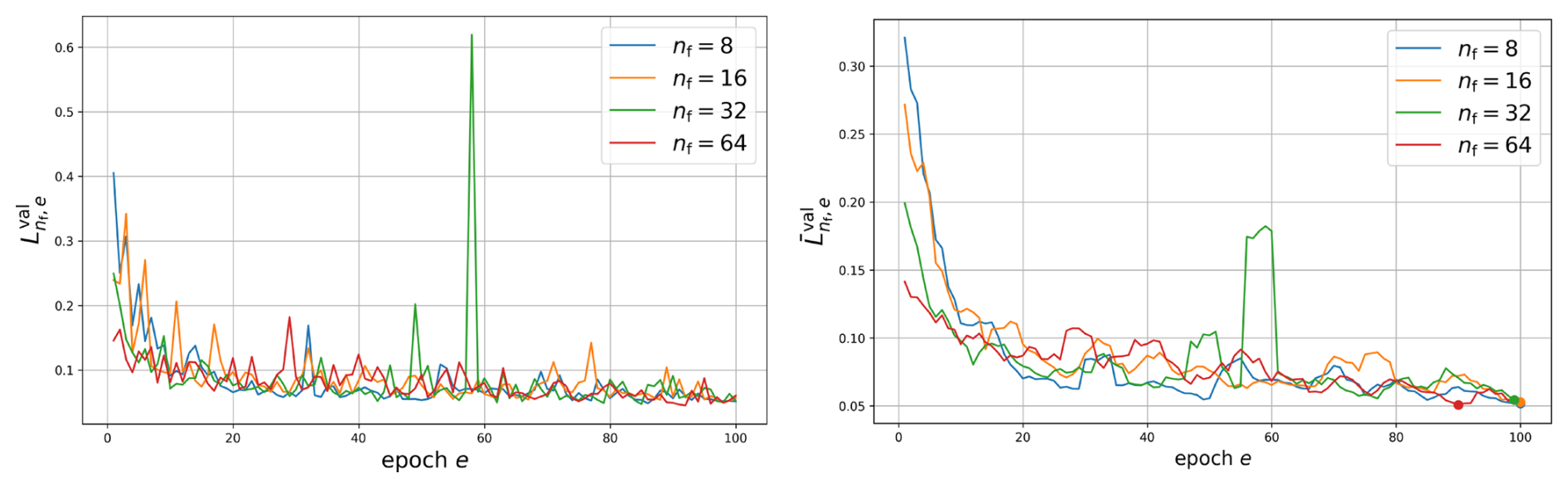
Figure 8 Validation loss $L_{n_{\mathrm{f}},e}^{\mathrm{val}}$ (left) and its moving average ${\stackrel{\mathrm{‾}}{L}}_{n_{\mathrm{f}},e}^{\mathrm{val}}$ (right) over the epochs e for each number of feature channels $n_{\mathrm{f}}\in \mathit{\{}\mathrm{8},\mathrm{16},\mathrm{32},\mathrm{64}\mathit{\}}$.

Figure 8 shows the validation losses $L_{n_{\mathrm{f}},e}^{\mathrm{val}}$ and their moving averages ${\stackrel{\mathrm{‾}}{L}}_{n_{\mathrm{f}},e}^{\mathrm{val}}$ during training for the four networks with $n_{\mathrm{f}}\in \mathit{\{}\mathrm{8},\mathrm{16},\mathrm{32},\mathrm{64}\mathit{\}}$ feature channels. The smallest moving average of the validation loss is attained by the network with n_f=64 feature channels after 90 epochs, i.e., with $n_{\mathrm{f}}^{\ast }=\mathrm{64}$ and $e^{\ast }=\mathrm{90}$. Its trainable parameters ${\mathit{\theta }}^{\ast }={\mathit{\theta }}_{\mathrm{64},\mathrm{90}}$ are used in the following evaluation.

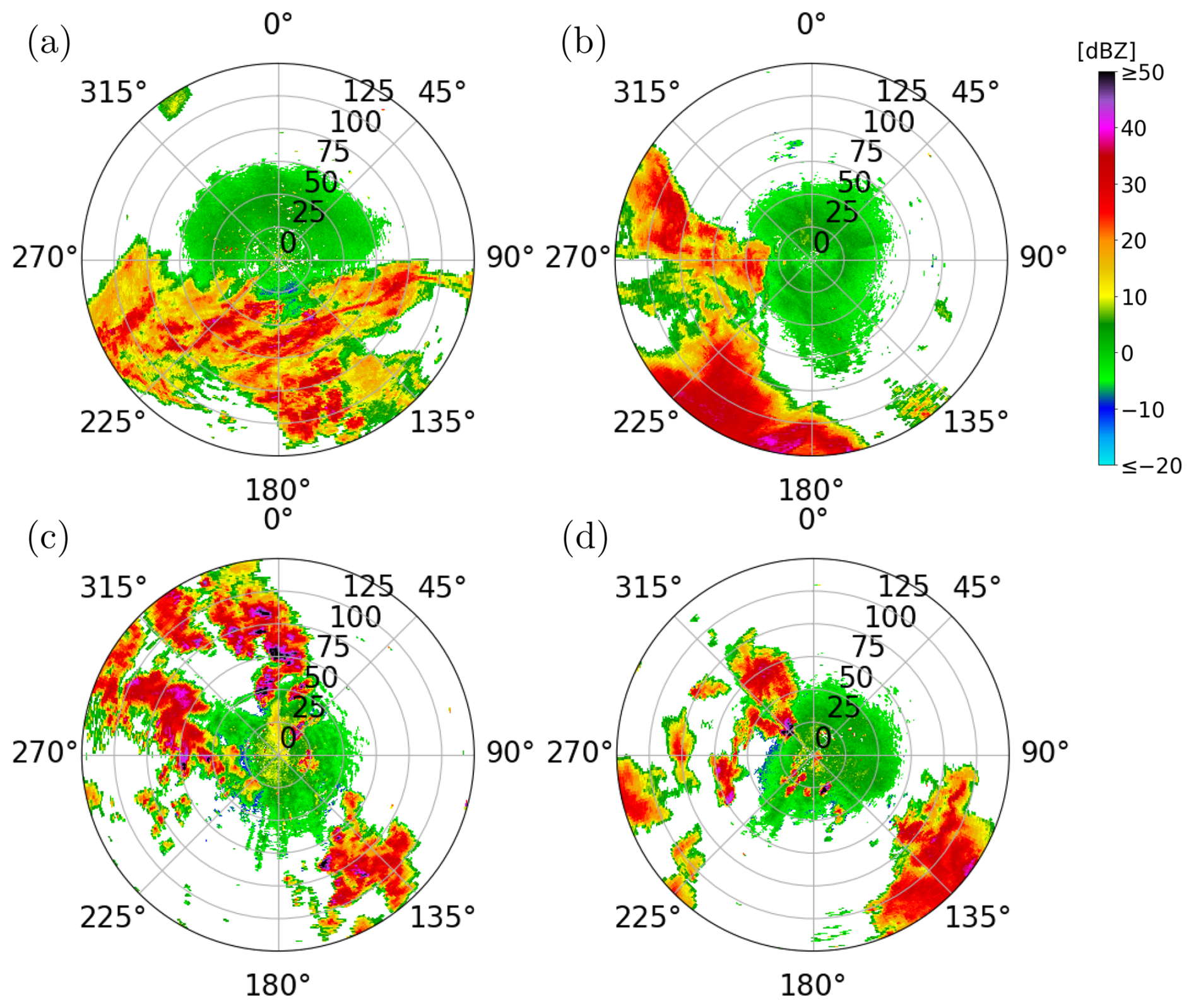
Figure 9 Overview of four of the five DBZH radar images in the test dataset ${\mathcal{D}}_{\exp }^{\mathrm{m}}$. The radar images shown were measured (a) on 5 June 2022, at 09:00 UTC in Essen, (b) on 5 June 2022, at 09:00 UTC in Neuhaus, (c) on 30 June 2022, at 16:00 UTC in Neuheilenbach and (d) on 30 June 2022, at 16:00 UTC in Türkheim. The remaining radar image from ${\mathcal{D}}_{\exp }^{\mathrm{m}}$, which was measured on 16 June 2022, at 09:00 UTC in Dresden, is shown in Fig. 1b.

We evaluate the trained network using the metrics stated in Sect. 2.7 and compare its performance to the SotA method detailed in Sect. 3. Segmentation performance is quantified on training datasets ${\mathcal{D}}_{\mathrm{train}}^{\mathrm{m}}$, ${\mathcal{D}}_{\mathrm{train}}^{\mathrm{w}}$, and ${\mathcal{D}}_{\mathrm{train}}^{\mathrm{s}}$, and validation datasets ${\mathcal{D}}_{\mathrm{val}}^{\mathrm{m}}$, ${\mathcal{D}}_{\mathrm{val}}^{\mathrm{w}}$, and ${\mathcal{D}}_{\mathrm{val}}^{\mathrm{s}}$, as introduced in Sect. 2.5. Moreover, both methods are also evaluated on a test dataset ${\mathcal{D}}_{\exp }^{\mathrm{m}}$ of experimentally measured mixed radar images, given by

$${\mathcal{D}}_{\exp }^{\mathrm{m}}=\mathit{\left\{}\right(A_n,G_n):n\in \mathit{\{}\mathrm{1},\mathrm{\dots },\mathrm{5}\mathit{\left\}}\mathit{\right\}},$$

where A_n∈D are radar images measured in June 2022 featuring both meteorological and non-meteorological echoes, and $G_n\in \mathit{\{}\mathrm{0},\mathrm{1}{\mathit{\}}}^{n_{\mathrm{r}}\times n_{\mathrm{a}}}$ are the corresponding ground truth images, which were manually labeled by a subject expert. Two of the five images were measured at 09:00 UTC on 5 June 2022 (radar stations Essen and Neuhaus), one at 09:00 UTC on 16 June 2022 (Dresden), and two at 16:00 UTC on 30 June 2022 (Neuheilenbach and Türkheim). The five test images are shown in Figs. 9 and 1b. They were selected to cover a variety of scenarios: stratiform and convective precipitation, convection close to the radar and at longer ranges, morning and afternoon data, and different radars. The test dataset ${\mathcal{D}}_{\exp }^{\mathrm{m}}$ was not used for training or model selection. However, the test image from June 16 was measured during the one-hour period from which the reflectivity weighting factor in Sect. 2.4 is determined.

Table 2 Area-weighted performance metrics for the evaluation of the trained network and the SotA method. Precision PRE^c and recall REC^c are computed for meteorological (c=0) and non-meteorological echoes (c=1). For the test dataset, the better value of the two methods is printed in bold.

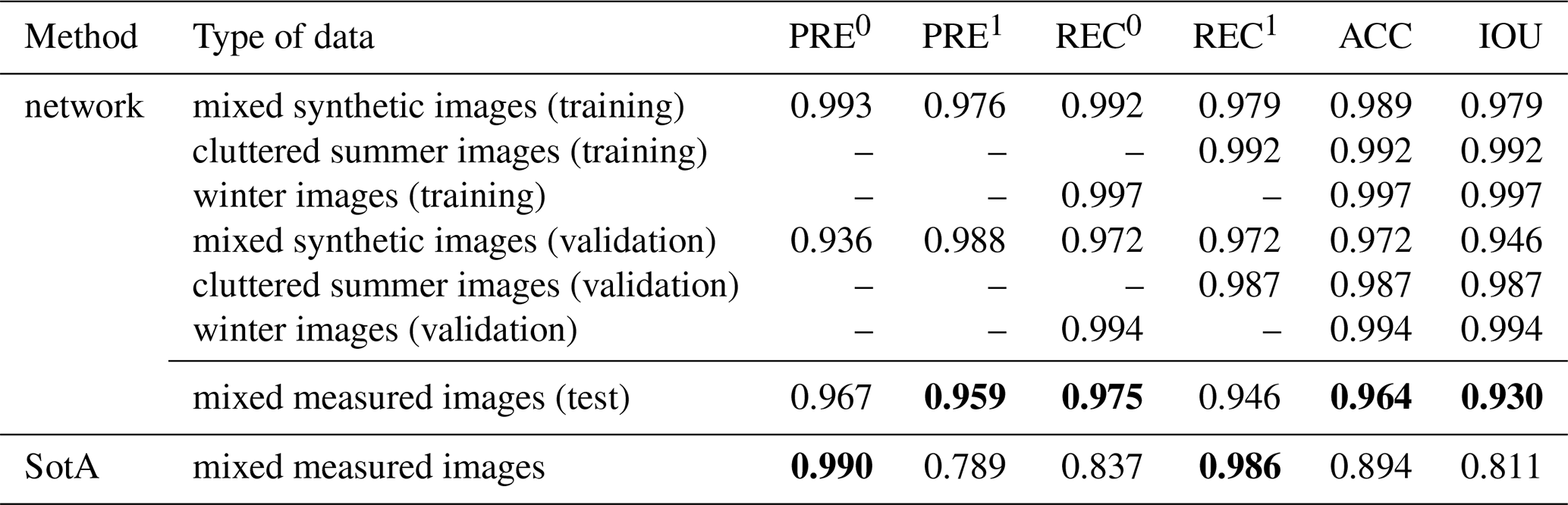
Table 2 shows a comparison of the resulting metrics averaged over the respective datasets as described in Sect. 2.7. The overall performance metrics on the validation datasets are slightly lower than those on the training datasets. The accuracy ACC and intersection over union IOU on the mixed validation dataset ${\mathcal{D}}_{\mathrm{val}}^{\mathrm{m}}$ are 0.972 and 0.946, respectively, compared to 0.989 and 0.979 on the mixed training dataset ${\mathcal{D}}_{\mathrm{train}}^{\mathrm{m}}$.

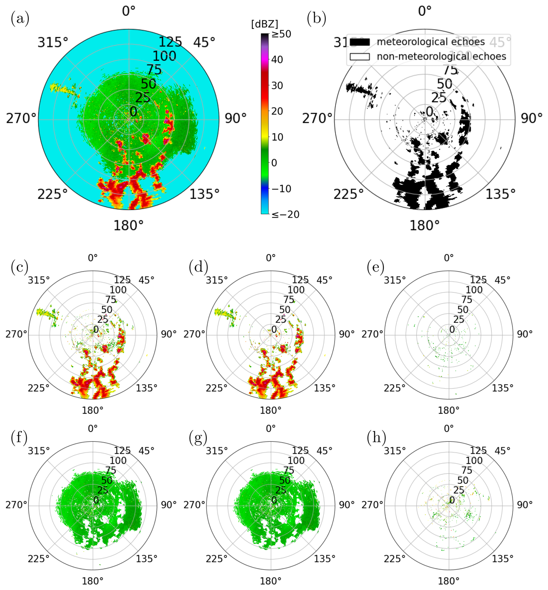
Figure 10 Evaluation of the network on a synthetic validation image: (a) input image and (b) corresponding ground truth, (c) pixels classified as meteorological echoes by the network, (d) correctly classified meteorological echoes, and (e) meteorological echoes misclassified as non-meteorological echoes. The bottom row shows (f) pixels classified as non-meteorological echoes, (g) correctly classified non-meteorological echoes, and (h) non-meteorological echoes misclassified as meteorological echoes. The radar image shown was generated using two radar images measured on 9 January 2025, at 17:05 UTC and on 18 June 2022, at 10:55 UTC in Essen.

Figure 10 visualizes the echoes that were correctly and incorrectly classified by the network for one mixed validation image in dataset ${\mathcal{D}}_{\mathrm{val}}^{\mathrm{m}}$. Most of the meteorological echoes, particularly those with high reflectivity, were correctly identified. This aligns with the recall value REC⁰ for meteorological echoes of 0.972 on dataset ${\mathcal{D}}_{\mathrm{val}}^{\mathrm{m}}$. Moreover, the resulting segmentation does not show any notable holes within areas surrounded by meteorological echoes. However, as can be seen in Fig. 10c, misclassified non-meteorological echoes are clearly visible as small speckles, leading to a lower precision value PRE⁰ for meteorological echoes of 0.936.

Table 3 Evaluation of the trained network and the SotA method. The table shows the area-weighted performance metrics for each of the five radar images of the test dataset ${\mathcal{D}}_{\exp }^{\mathrm{m}}$. Precision PRE^c and recall REC^c are computed for meteorological (c=0) and non-meteorological echoes (c=1). For each radar image, the better value of the two methods is printed in bold.

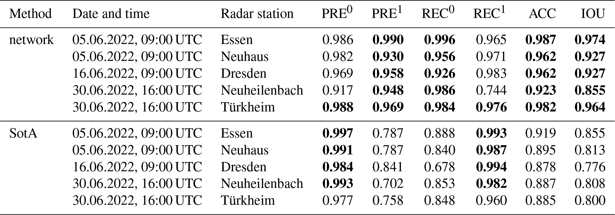
When evaluated on the experimentally measured mixed dataset ${\mathcal{D}}_{\exp }^{\mathrm{m}}$, the network performance is comparable to that on the validation dataset, with accuracy ACC and intersection over union IOU of 0.964 and 0.930, respectively. However, when evaluating the SotA method on the same mixed dataset ${\mathcal{D}}_{\exp }^{\mathrm{m}}$, it performs substantially worse, with accuracy ACC and intersection over union IOU of 0.894 and 0.811, respectively. These overall differences are caused by larger differences in precision PRE¹ for non-meteorological echoes and recall REC⁰ for meteorological echoes, where the SotA method achieves scores of 0.789 and 0.837, respectively, compared to the neural network with scores of 0.959 and 0.975. The SotA method achieves better scores for recall REC¹ for non-meteorological echoes and precision PRE⁰ for meteorological echoes, with values of 0.986 and 0.990, respectively, compared to the neural network with scores of 0.946 and 0.967. Table 3 shows the performance metrics for each of the five radar images of the test dataset ${\mathcal{D}}_{\exp }^{\mathrm{m}}$. The intersection over union IOU of the network ranges from 0.855 (Neuheilenbach) to 0.974 (Essen). For each labeled radar image, the intersection over union IOU and the accuracy ACC are higher than the respective values for the SotA method.

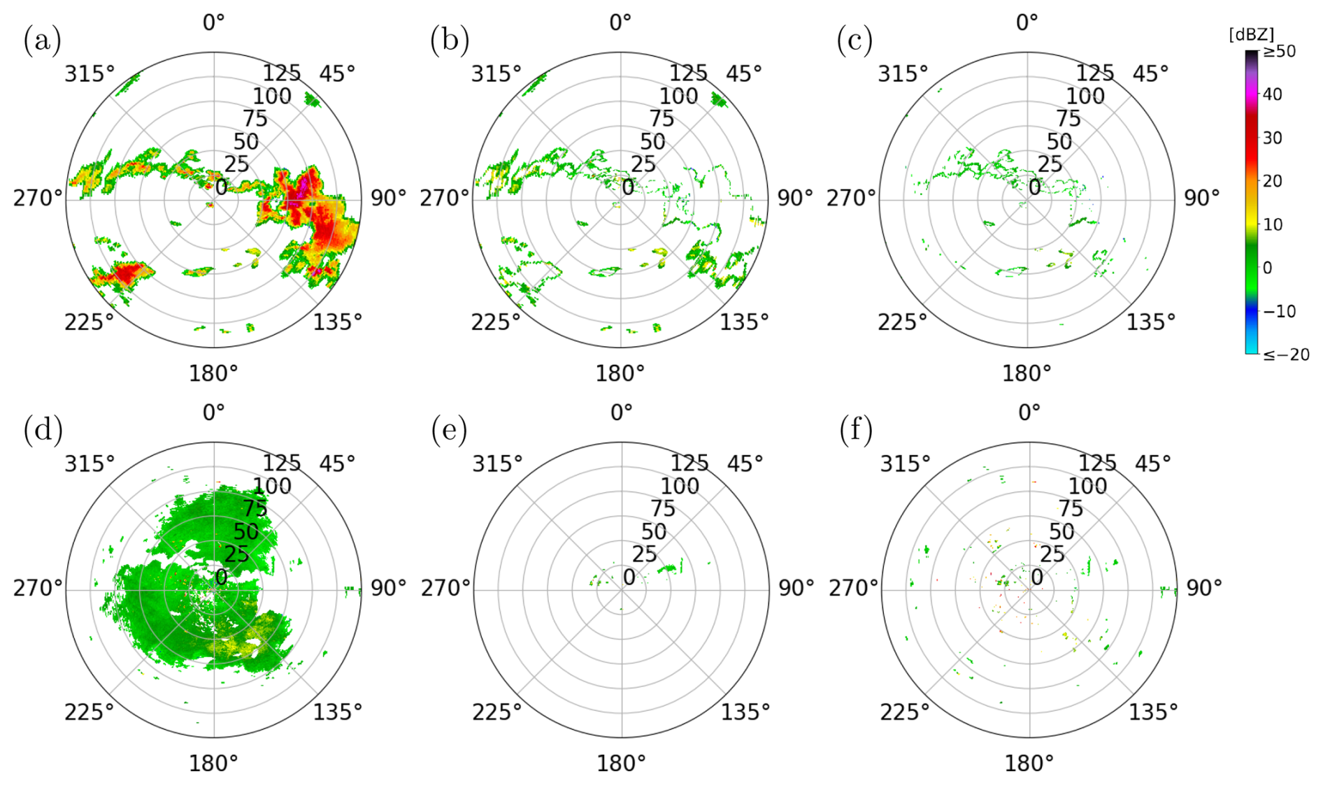
Figure 11 Evaluation of the SotA method and the trained network on the experimentally measured radar image shown in Fig. 1b: The first row shows (a) the ground truth for the meteorological echoes and the meteorological echoes misclassified as non-meteorological echoes by (b) the SotA method and (c) the trained network. Analogously, the second row shows (d) the hand-labeled ground truth for the non-meteorological echoes and the non-meteorological echoes misclassified as meteorological echoes by (e) the SotA method and (f) the trained network.

Figure 11 shows the incorrectly segmented echoes of the network (Fig. 11c and f) and of the SotA method (Fig. 11b and e) for one experimentally measured mixed radar image in dataset ${\mathcal{D}}_{\exp }^{\mathrm{m}}$. The top row shows the incorrect segmentations of meteorological echoes for both methods, with the neural network making substantially fewer errors. Here, the SotA method tends to incorrectly classify the pixels located at the boundary of weather events. However, the SotA method performs substantially better in correctly identifying non-meteorological echoes near the radar station.

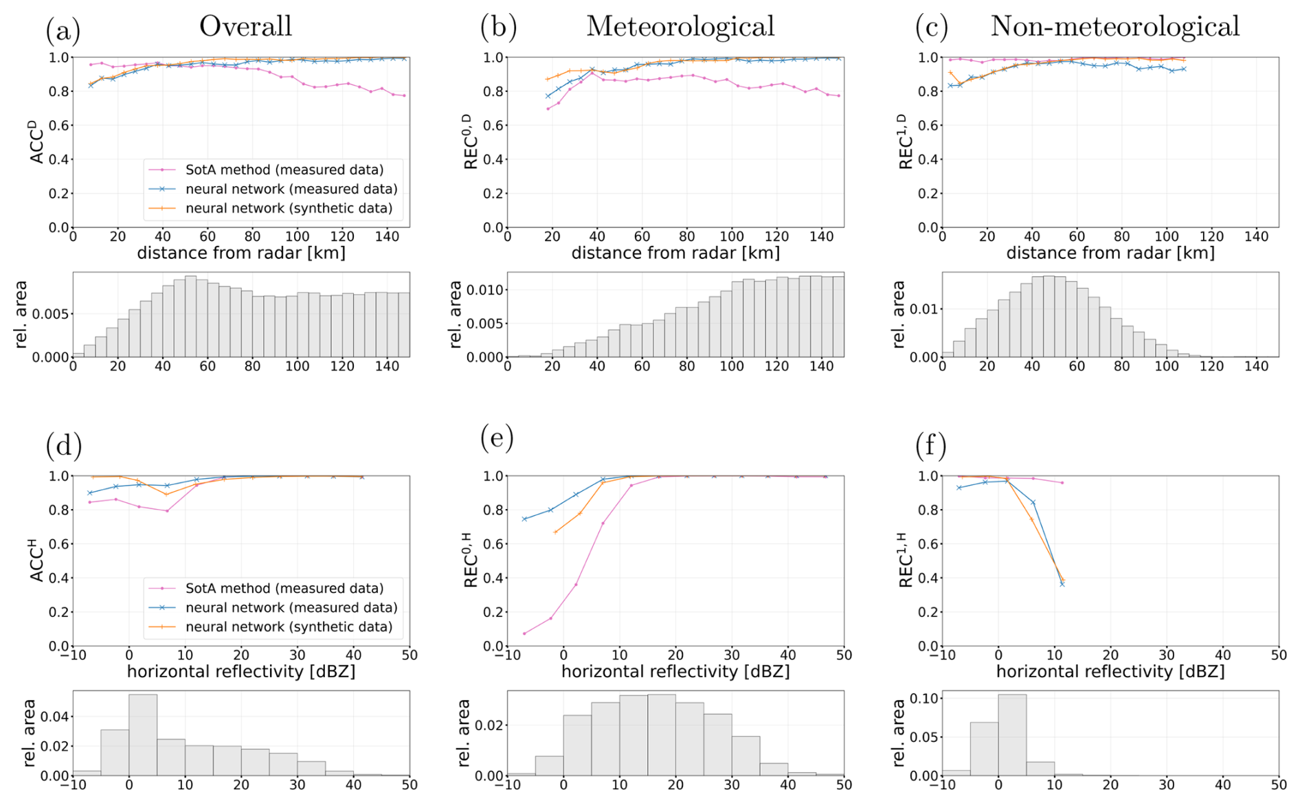
Figure 12 First row: Accuracy in dependence on the distance from the radar for shows the incorrectly segmented echoes of the (a) meteorological and non-meteorological echoes combined, (b) meteorological echoes, and (c) non-meteorological echoes, as classified in the ground truth. Second row: Accuracy in dependence on the horizontal reflectivity values for the same three sets of pixels. The metrics are only shown for distances and horizontal reflectivities with a relative area greater than 0.0005, respectively. The histograms below show the area distribution for each of the three sets of pixels, respectively. The SotA method was evaluated on the experimentally measured mixed dataset ${\mathcal{D}}_{\exp }^{\mathrm{m}}$ and the neural network was evaluated on the same experimentally measured dataset and additionally on the mixed validation dataset ${\mathcal{D}}_{\mathrm{val}}^{\mathrm{m}}$.

In order to further investigate this, Fig. 12a shows the accuracy depending on the distance, while Fig. 12b and c show the class-specific recall scores for meteorological and non-meteorological echoes, respectively. The network's accuracy ACC^D on the test dataset ${\mathcal{D}}_{\exp }^{\mathrm{m}}$ increases with distance from the radar, rising from below 0.9 within 25 km to nearly 1.0 beyond 75 km. The same trend can be observed for the validation dataset ${\mathcal{D}}_{\mathrm{val}}^{\mathrm{m}}$, for which only slightly higher scores are achieved by the network. When compared to the SotA method, the recall REC^0,D for meteorological echoes depending on distance is higher for the network than for the SotA method for all distances, and the opposite is true for non-meteorological echoes. The most substantial differences occur close to the radar, at a distance of less than 25 km, where the neural network achieves a recall REC^1,D of 0.885, compared to that of the SotA method with 0.981. This relatively lower recall close to the radar quantifies the errors we see in Fig. 11f, where a substantial number of non-meteorological echoes near the radar are incorrectly classified. When considering the recall REC^0,D for meteorological echoes depending on distance, the network clearly outperforms the SotA method at distances further from the radar, with a recall value of 0.986 compared to that of the SotA method with 0.831 beyond 75 km. The echoes further away from the radar represent a proportionally larger area, as shown in the histograms, and thus the network outperforms the SotA method overall.

Analogously, we evaluate the accuracy and class-specific recall in dependence on the horizontal reflectivity values, as shown in Fig. 12d to f. For meteorological echoes with a reflectivity higher than 10 dBZ, both the network and the SotA method achieve a recall REC^0,H near 1.0. However, for horizontal reflectivities below 10 dBZ, the SotA performance degrades substantially, whereas the network maintains a recall of 0.925. While meteorological echoes with reflectivity values below 0 dBZ are rare in the dataset, those with reflectivity values between 0 and 10 dBZ are much more frequent, as shown in the histogram of Fig. 12e. For example, the edges of weather events are typically less reflective and are often incorrectly classified as non-meteorological echoes by the SotA method, as shown in Fig. 11b. In the case of non-meteorological echoes, the network struggles to classify echoes with high reflectivity (>10 dBZ), achieving a lower recall REC^1,H of 0.308 compared to the SotA method, which achieves a recall value of 0.961. Nevertheless, such high-reflectivity non-meteorological echoes are rare in the dataset.

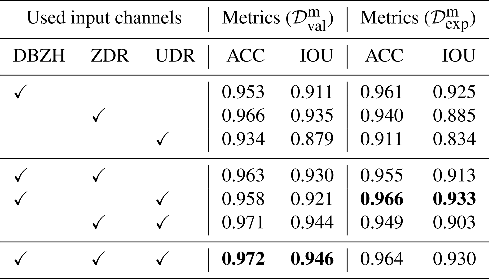
To investigate the influence of the individual input channels, one network is trained for each of the seven combinations of the DBZH, ZDR, and UDR channels. All networks are trained on the same synthetic training data and with the same hyperparameters as described in Sect. 2.5, where the number of feature channels is fixed to n_f=64 and the number of training epochs is selected based on the validation loss as described in Sect. 2.6.

Table 4 shows the resulting performance metrics on the mixed validation dataset ${\mathcal{D}}_{\mathrm{val}}^{\mathrm{m}}$ and the test dataset ${\mathcal{D}}_{\exp }^{\mathrm{m}}$, where the row using all three channels corresponds to the network considered previously. Among the networks using a single input channel, the network using the DBZH channel achieves the highest metrics on the test dataset. The highest metrics are achieved by the network combining the DBZH and UDR channels, with an accuracy of 0.966 and an intersection over union of 0.933 on the test dataset. When DBZH and UDR channels are considered, the ZDR channel does not appear to improve performance on the test dataset. Since UDR is deduced from ZDR and ρ_HV, this result suggests that the ρ_HV contributions to UDR add to the performance, whereas using both UDR and ZDR does not further improve the performance.

Table 4 Area-weighted accuracy ACC and intersection over union IOU for the trained networks in dependence on the input channels used. The networks are evaluated on the mixed validation dataset ${\mathcal{D}}_{\mathrm{val}}^{\mathrm{m}}$ and the test dataset ${\mathcal{D}}_{\exp }^{\mathrm{m}}$. The best value in each column is printed in bold.

5 Discussion

The results presented in Sect. 4 demonstrate that a neural network is capable of effectively identifying non-meteorological echoes in radar images. One of the most significant findings is the network's ability to generalize from synthetically generated radar images to experimentally measured mixed radar images ${\mathcal{D}}_{\exp }^{\mathrm{m}}$. Although the training process relied exclusively on synthetically generated radar images, network performance on experimentally measured radar images was in line with, or exceeding, that of the SotA method currently used at DWD.

A key advantage of the proposed network-based method over the SotA method used at DWD lies in the preservation of meteorological echoes, particularly at the boundaries of weather events and in regions of weak precipitation. As illustrated in Fig. 11b, and quantified in Fig. 12e, the SotA method tends to incorrectly classify the boundaries of weather events as non-meteorological echoes. This is likely due to the SotA method's reliance on heuristically chosen thresholds and local neighborhood statistics (e.g., 3×3 or 5×5 neighborhoods). In contrast, the network utilizes context from a larger neighborhood, allowing it to better recognize the spatial structures of weather events.

However, the evaluation also highlighted limitations that should be addressed in future work. The network showed a lower recall REC¹ for non-meteorological echoes compared to the SotA method, particularly for radar gates close to the radar at distances of less than 25 km, as shown in Fig. 12c. The network's errors are likely a consequence of the underlying winter radar images used for training. For the generation of mixed synthetic radar images, we assign echoes in winter radar images exclusively as meteorological echoes. However, in reality, the winter radar images also contain non-meteorological echoes, particularly in areas close to the radar, as can be seen in Fig. 3. Consequently, the corresponding pixels are incorrectly labeled as meteorological in the ground truth. Therefore, the network may be disincentivized from correctly identifying non-meteorological echoes near the radar during training. A quantitative verification of this explanation, as well as possible improvements of the network's performance near the radar, is left for future work.

The contributions of the individual input channels are investigated by the ablation study in Sect. 4, see Table 4. As expected, the horizontal reflectivity appears the most informative radar moment, with an intersection over union of 0.925 on the test dataset, compared to 0.885 for ZDR and 0.834 for UDR. For the depolarization ratio, it was unclear whether the synthetic UDR images are useful for training at all, since each of their values is taken from only one of the two combined radar images, see Sect. 2.4. However, appending the UDR channel to the DBZH channel increases the intersection over union on the test dataset to 0.933. Moreover, the network trained using this combination performs similarly on the validation dataset, with an intersection over union of 0.921. This suggests that what the network learns from the synthetic UDR images transfers to experimentally measured radar images. In addition, this result suggests that a physically interpretable combination method is not necessarily required for an input channel to be useful. Additional radar moments could therefore be included in the training data by the same simple assignment used for the synthetic UDR images, even if a physically motivated mixing of two radar images is not available. In particular, Doppler-based moments, such as the radial velocity or the clutter correction moment used by the SotA method, are promising candidates.

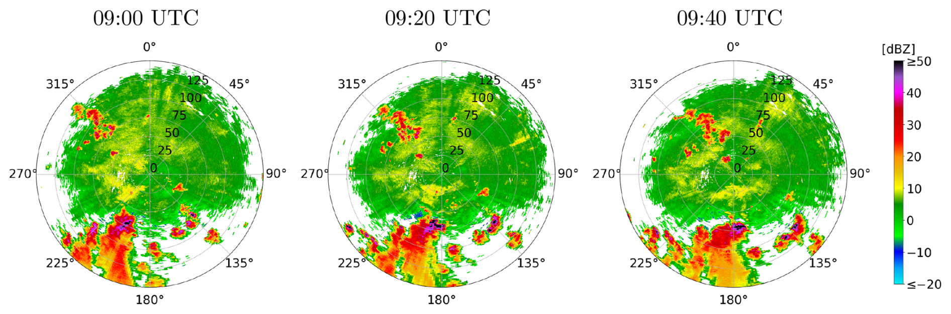
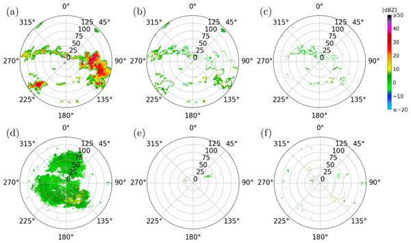
Figure 13 Time series of mixed summer radar images collected at the same radar station at 20 min intervals. The radar images shown were measured on 16 June 2022 in Isen.

Regarding the model's generalizability, the evaluation results indicate that the network did not suffer from substantial overfitting during training. The overall performance metrics on the mixed training dataset ${\mathcal{D}}_{\mathrm{train}}^{\mathrm{m}}$ are similar to those observed on the mixed validation dataset ${\mathcal{D}}_{\mathrm{val}}^{\mathrm{m}}$ and the test dataset ${\mathcal{D}}_{\exp }^{\mathrm{m}}$. The mixed training data ${\mathcal{D}}_{\mathrm{train}}^{\mathrm{m}}$ was generated by combining cluttered summer radar images measured on 18 June 2022 (10:00–11:00 UTC) with winter radar images measured on 9 January 2025 (17:00–18:00 UTC). The weighting factors λ_w and λ_s used to combine these were explicitly calibrated so that the generated images resembled mixed summer radar images measured on 16 June 2022 (09:00–10:00 UTC). The validation datasets were generated from radar images of the same time periods, measured at a radar station that was not used for training, see Sect. 2.5. In contrast, the test dataset ${\mathcal{D}}_{\exp }^{\mathrm{m}}$ consists of five experimentally measured mixed radar images from three different days. Four of them were measured on 5 and 30 June 2022, i.e., on days from which no radar data was used for the generation of the synthetic training data, and the two images from 30 June were measured in the afternoon (16:00 UTC). The remaining test image was measured on 16 June 2022, during the one-hour period from which the weighting factors were determined. The test dataset contains a variety of stratiform and convective precipitation, close to the radar and at longer ranges. The network performed well on all five test images, see Table 3. This indicates that the network transfers to experimentally measured summer images of other days and times of day, although robustness across seasons and event types cannot be established with five images from three summer days. Moreover, all meteorological echoes in the training data are taken from the winter radar images. Artifacts, such as differential attenuation, that occur in strong summertime convection are therefore absent from the training data. The five test images are unlikely to represent the wide range of such rare artifacts, and evaluating the performance of the network on them requires a larger amount of test data. To further enhance and evaluate the network's generalization capabilities, future work should incorporate data from a broader range of meteorological situations. Despite the very limited amount of data for training, the network already shows good performance. For operational purposes, the training dataset will have to be extended substantially, such that it incorporates all kinds of possible meteorological situations and artifacts. For example, summer-only artifacts could be incorporated by partially labeling a small number of radar images in which they occur, or by generating them synthetically.

There are several improvements to the proposed method. First, as seen in Fig. 10, the network output includes isolated misclassified pixels. Applying a post-processing despeckle filter, similar to the one described in Sect. 2.2 for the input data, could remove these small artifacts and further improve precision without adding methodological complexity. Second, the current approach processes radar images from a single elevation angle and time step. Incorporating additional elevation angles or time steps could provide the network with additional spatially-resolved or time-resolved structural information. Although this would add significant complexity to the proposed methodology, it represents a very promising adjustment. For one, non-meteorological echoes are less common at higher elevation angles, whereas weather events often extend vertically. Furthermore, incorporating time-resolved information would allow the network to exploit differences in movement patterns. For example, insects are typically either stationary or move irregularly, whereas weather events exhibit coherent motion (Fig. 13).

6 Conclusions

Accurate identification of non-meteorological echoes in radar images is a prerequisite for reliable quantitative precipitation estimation, hydrometeor classification and aviation safety. In this work, we introduced a deep learning approach using a U-net architecture to segment dual-polarization weather radar data. To overcome the scarcity of pixel-wise labeled training data, we developed a novel method for generating synthetic training data by combining winter data and cluttered summer data.

The proposed method was evaluated against a state-of-the-art (SotA) method currently used at Deutscher Wetterdienst. Our results show that the neural network outperforms the SotA method in preserving weak precipitation and the boundaries of weather events, achieving an overall accuracy of 0.964 and an intersection over union of 0.930, compared to 0.894 and 0.811 for the SotA method on five expert-labeled radar images.

Most importantly, this study demonstrates that synthetically generated radar moments can be used for training deep neural networks in order to accurately identify non-meteorological echoes. Despite being trained exclusively on synthetically generated mixed radar data, the network accurately identified non-meteorological echoes in experimentally measured mixed radar data without any further fine-tuning.

To ensure robustness across the entire year, future work should incorporate data from spring and autumn to capture seasonal variations. Furthermore, the neural network's capabilities could be extended beyond 2D spatial features. Utilizing consecutive time steps or multiple elevation angles as input could provide the time-resolved and volumetric context needed for even more precise segmentation.