Review of the Radon Tracer Method for GHG emission estimates: development, application guidelines, improvements, and caveats

The Radon Tracer Method (RTM) is an established, independent top-down method that can be used to cross-check bottom-up greenhouse gas (GHG) emission estimates. Furthermore, as uncertainties of Atmospheric Transport Models are reduced, the RTM can provide a convenient means of quantifying continual improvement of inversion-based top-down GHG emission estimates. While the accessibility and perceived simplicity of the RTM drive its popularity, the technique is better suited to assessing long-term relative changes in GHG emissions than absolute changes, due to short-term soil moisture influences on simulated radon flux uncertainty. Considerations for applying the RTM, based on fundamental assumptions of the technique's development, are application and season specific, making the development of a “standard protocol” for its use challenging. After proposing a novel alternative means of applying the nocturnal accumulation RTM, which improves interpretation of findings, we use measurements from a range of contrasting sites to discuss the significance of the technique's eight key considerations: (i) nocturnal window definition, (ii) radon and target gas accumulation thresholds, (iii) radon-to-target gas regression linearity thresholds, (iv) measurement height, (v) the contributing fetch, (vi) spatial and temporal radon flux variability, (vii) RTM temporal resolution, and (viii) application specific selection of a suitable radon monitor. The insight provided by these examples to the flexibility (or otherwise) of the technique's considerations will clarify the implications if users choose to relax or ignore them, potentially making future RTM studies more directly comparable.

1 Introduction

Global temperatures have increased ∼ 1.5 °C over the past 150 years; mostly in the past 50 years (CSIRO, 2024). To put this in perspective, the average rate of natural warming since the last glacial maximum (20–25 ka BP) has been ∼ 1.0 °C per 3500 years (Tierney et al., 2020). Ice core analyses and atmospheric baseline monitoring (e.g. Neftel et al., 1985; Etheridge et al., 1998; Thoning et al., 1989; https://gml.noaa.gov/ccgg/trends/, last access: 7 April 2025), demonstrate that the greatest contribution to recent accelerated warming has been anthropogenic greenhouse gas (GHG) emissions, through processes including power generation, transportation, deforestation, agriculture (including animal farming), waste treatment, manufacturing, and heating (Schleussner et al., 2016).

With very low uncertainty, profound natural and anthropogenic ecosystem alterations through sea level rise, extreme weather events, increased severity of droughts and flooding, terrestrial and aquatic biodiversity loss, and unprecedented risks to vulnerable persons and populations through heatwaves and loss of food security, have already been ascribed to anthropogenic climate change (Allen et al., 2018). Left unchecked, the United Nations Intergovernmental Panel on Climate Change (IPCC) warns of increased severity of such impacts.

A key objective of the United Nations Framework Convention on Climate Change's 2015 Paris Agreement was therefore to hold the increase in global temperature less than 2 °C above pre-industrial levels, and to pursue efforts to limit warming to the ∼ 1.5 °C already observed (Bergamaschi et al., 2018a). Key to achieving this goal is a requirement for member countries to submit national climate action plans and long-term low GHG emission development strategies, report transparently on actions taken to progress climate change mitigation and establish carbon neutrality targets.

A necessary step in demonstrating the need for, and future efficacy of, GHG-related climate mitigation is an improved understanding of local- to regional-scale GHG emissions and a reliable way of tracking changes in their emission rates over the years to come. Traditionally, GHG emission estimates relied on bottom-up (BU) inventories, developed through IPCC approved methods, based on statistical activity information and source specific emission factors (Bergamaschi et al., 2018a). However, large uncertainties exist in these emission factors, based on the completeness of knowledge about all contributing sources, the accuracy of reported anthropogenic sources (Bergamaschi et al., 2018b; Cheewaphongphan et al., 2019), upscaling of anthropogenic source information, and present understanding of natural sources and feedback mechanisms associated with ongoing climate change.

For independent assessment of BU inventories, top-down (TD) approaches for GHG emission estimates have been developed. The combination of high-quality in situ or remote atmospheric GHG observations with Atmospheric Transport Models (ATMs) for inverse modelling has become a popular tool for this purpose (Witi and Romano, 2019; Petrescu et al., 2021; Manning et al., 2021; Bukosa et al., 2025). However, this approach requires considerable computational resources, and large ATM uncertainties under certain conditions (often associated with local-scale vertical mixing at sub-grid resolution) limit the accuracy of results (van der Laan et al., 2010; Levin et al., 2011; Bergamaschi et al., 2018b; Schuh et al., 2019; Lian et al., 2021; Manning et al., 2021; Kikaj et al., 2025a).

A less resource intensive TD technique for emission estimates is the Radon Tracer Method (RTM) (Levin, 1987). Four implementations of the RTM have appeared in the literature, each targeting different spatial scales and temporal resolutions of emission estimates: (i) a regional-to-continental scale approach (e.g. Levin, 1987; Levin et al., 2003; Schmidt et al., 1996, 2001; timescale weeks to months); (ii) a regional scale plume/event-based approach (e.g. Wilson et al., 1997; Biraud et al., 2000; Messager et al., 2008; Wada et al., 2010; timescale hours to days); (iii) a local-to-regional scale nocturnal accumulation approach (e.g. Levin et al., 1999, 2011, 2021; Schmidt et al., 2001; Hammer and Levin, 2009; Vogel et al., 2012; van der Laan et al., 2014; Grossi et al., 2018; timescale daily); and, (iv) a local scale profile method (e.g. Conen et al., 2002; Martens et al., 2004; Obrist et al., 2005; timescale daily). Here, in part fulfilment of a goal of the EMPIR project 19ENV01 traceRadon (Röttger et al., 2021), and in support of revising the IG3IS Urban Greenhouse Gas Emission Observation and Monitoring Good Research Practice Guidelines (Turnbull et al., 2025), we focus exclusively on method (iii) the local-to-regional nocturnal accumulation implementation of the RTM (henceforth, “the RTM”), which has been the most commonly adapted in the literature.

Since its development (Levin, 1987), the RTM has grown in popularity due to: (i) the perceived simplicity of its application, (ii) its accessibility (scant need of high-performance computational hardware or excessive supporting measurement infrastructure), and (iii) the increased availability of high quality, long-term atmospheric radon observations. In recent years, however, it has sometimes been applied to situations for which it is not well suited, often with insufficient discussion of consequences. Also, in the hope of improving data coverage, there has been insufficient reverence for key data selection criteria, without suitable discussion regarding the potential impact of these decisions on reported findings.

A “standard protocol” for application of the RTM (a goal of the traceRadon project) would facilitate interpretation results and make findings more comparable between studies. However, considerations for applying the RTM are strongly site and season specific, making the development of one standard protocol impractical. Typically, each existing RTM study only discusses a subset of assumptions or considerations for the technique that are specific to the site in question, making it challenging for new users to fully appreciate the strengths and weaknesses of the technique when applied to a new situation. Here we have endeavoured to create an exhaustive list of assumptions and considerations for applying the RTM based on observations from a variety of contrasting measurement sites (note summary in Appendix A). It is our intention that, equipped with this information, future users will more easily develop an understanding of the flexibility (or inflexibility), of the underlying assumptions and considerations of the technique, and be in a better position to judge (and discuss) the impact on their results of choosing to relax, or ignore, these considerations to suit their specific measurement needs.

Compounding the occasional inconsistencies in contemporary RTM applications, Levin et al. (2021) challenged a long-standing assumption of the RTM that has contributed to its perceived simplicity: the temporal consistency and homogeneity of the terrestrial radon flux. Comparing long-term observed radon fluxes with simulated values, Levin et al. (2021) demonstrated large potential uncertainties in RTM applications arising from soil moisture-related changes in the radon flux on synoptic (days) to seasonal (months) timescales. In the absence of long term, distributed radon flux measurements, these findings highlight that in general the RTM is more suitable for assessing long-term relative changes in tracer emissions than short-term absolute values, which is significant when comparing results from RTM and other TD or BU techniques.

This technique review paper aims to build upon the work of Levin et al. (2021) in outlining the strengths and weaknesses of the RTM. We expand the list of considerations for applying the technique, provide more detail regarding their significance, offer an alternative way to implement the RTM that improves interpretation of findings, and provide evidence of a need – in some cases – to revisit contemporary RTM footprint determination techniques.

2 Methods

2.1 Nocturnal accumulation RTM – original derivation

As has been established (Levin, 1987; Levin et al., 1999; Schmidt et al., 2001), any conservative trace gas with a distributed, relatively consistent, near-surface source, will accumulate beneath the capping inversion of a Stable Nocturnal Boundary Layer (SNBL) over land between sunset and sunrise.

To characterise this accumulation, a simplified 1-D representation is traditionally considered: an atmospheric column of unit cross section that experiences negligible advection through its walls (equivalent to requiring homogeneous fluxes over the contributing fetch), with an impermeable “lid” at a height H above the surface. Conditions that are most closely met under stable nocturnal conditions over flat terrain, characterised by a strong, low, thermal inversion and low surface wind speeds.

After sunset, the change in concentration of a target gas (C_g), over a time interval (t), measured within the column at a fixed height z above the surface (z<H), is solely dependent on its surface flux (F_g) and the height of the box.

$$\begin{array}{}\text{(1)}& {\displaystyle \frac{\mathrm{d}{C}_{\mathrm{g}}\left(t\right)}{\mathrm{d}t}}={\displaystyle \frac{F_{\mathrm{g}}}{H\left(t\right)}},\end{array}$$

When modelling this scenario however, the idealised atmospheric column extends to a height H^′(t), a “mixing length scale” (closely related to H), representative of the height of an equivalent atmospheric layer within which the target species emitted from the surface are assumed to mix instantly and uniformly (Griffiths et al., 2013).

The principles that underlie Eq. (1) apply equally to any conservative tracer with a near-surface source. ²²²Rn (radon) is a naturally occurring noble gas of terrestrial origin. It is not sufficiently soluble to be significantly impacted by rainfall or cloud processes on shorter than diurnal timescales, is not subject to dry deposition, and has a source function that is less spatially and temporal variable than other trace atmospheric species. Furthermore, while radon is radioactive, with a half-life of 3.8232(8) d, this timescale is long enough compared with mixing timescales in the Atmospheric Boundary Layer (ABL; ∼ 1 h) or a single night (≤ 12 h) for it often to be considered conservative. However, a decay term can easily be included in its budget.

$$\begin{array}{}\text{(2)}& {\displaystyle \frac{\mathrm{d}{C}_{\mathrm{Rn}}\left(t\right)}{\mathrm{d}t}}={\displaystyle \frac{F_{\mathrm{Rn}}}{H^{\prime }\left(t\right)}}-\mathit{\lambda }\cdot C_{\mathrm{Rn}}\left(t\right),\end{array}$$

where F_Rn represents the radon flux over the base of the atmospheric column, and $\mathit{\lambda }=\mathrm{0.00755}{\mathrm{h}}^{-\mathrm{1}}$ is the radon decay constant.

In practice, it is not common for the nocturnal inversion height to be known (since this requires costly profiling instrumentation or significant infrastructure, e.g. a tall tower), and this value typically varies over the course of a night. However, after making the following assumptions:

• i.

  the fluxes of both gases are similarly distributed and relatively homogeneous across the contributing fetch,

• ii.

  if heterogeneity does exist, it should be random, and on small spatial scales compared with the contributing fetch, and uncorrelated with atmospheric processes operating on small temporal/spatial scales,

• iii.

  the target gas has no significant sinks in the atmosphere over timescales associated with the measurement, or between the point of emission and measurement,

• iv.

  both species are acted upon by the same transport and mixing processes from the source to the point of measurement (which includes mixing to the same height), and

• v.

  both gases are measured at the same, constant location, and height above ground within the SNBL,

Schmidt et al. (2001) demonstrated that the unknown length scale H^′ can be eliminated by combining Eqs. (1) and (2), and solving for the flux of the target species:

$$\begin{array}{}\text{(3)}& F_{\mathrm{g}}=F_{\mathrm{Rn}}\cdot {\displaystyle \frac{\mathrm{d}{C}_{\mathrm{g}}\left(t\right)}{\mathrm{d}{C}_{\mathrm{Rn}}\left(t\right)}}\cdot {\left(\mathrm{1}+{\displaystyle \frac{\mathit{\lambda }\cdot C_{\mathrm{Rn}}\left(t\right)}{\frac{\mathrm{d}{C}_{\mathrm{Rn}}\left(t\right)}{\mathrm{d}t}}}\right)}^{-\mathrm{1}},\end{array}$$

Assuming $\mathit{\lambda }{C}_{\mathrm{Rn}}\ll \mathrm{d}{C}_{\mathrm{Rn}}/\mathrm{d}t$, which is often true for stable nights over land with shallow mixing layers since C_Rn is usually 10–20 Bq m⁻³ and $\mathrm{d}{C}_{\mathrm{Rn}}/\mathrm{d}t\mathrm{1}-\mathrm{2}\mathrm{Bq}{\mathrm{m}}^{-\mathrm{3}}{\mathrm{h}}^{-\mathrm{1}}$, Eq. (3) simplifies to (e.g. Schmidt et al., 2001; Hammer and Levin, 2009):

$$\begin{array}{}\text{(4)}& F_{\mathrm{g}}=F_{\mathrm{Rn}}\cdot {\displaystyle \frac{\mathrm{\Delta }{C}_{\mathrm{g}}\left(t\right)}{\mathrm{\Delta }{C}_{\mathrm{Rn}}\left(t\right)}}\cdot \left(\mathrm{1}-{\displaystyle \frac{\mathit{\lambda }\cdot C_{\mathrm{Rn}}\left(t\right)}{\frac{\mathrm{d}{C}_{\mathrm{Rn}}\left(t\right)}{\mathrm{d}t}}}\right),\end{array}$$

where Δ here represents the enhancement of the target gas (or radon) above an initial background value (e.g. the well-mixed concentration in the ABL before sunset), such that $\mathrm{\Delta }{C}_{\mathrm{g}}\left(t\right)=C_{\mathrm{g}}\left(t\right)-C_{\text{ABL}}$.

In practice, when applying the RTM over a single night (or part thereof), the ratio of the finite differences of the target gas and radon ($\mathrm{\Delta }{C}_{\mathrm{g}}/\mathrm{\Delta }{C}_{\mathrm{Rn}}$) is equivalent to the regression slope between the observed co-accumulating gases over the defined observation period (irrespective of their background values), where any mixing ratios have been converted to dry-air concentrations. The flux of the target gas is then retrieved by scaling the estimated radon flux from the contributing fetch by this slope.

Considering radon's half-life and potential nocturnal accumulation period (≤12 h), the term in brackets of Eq. (4) results in only a small modification of the estimated flux of the target gas. Mindful of the uncertainties already associated with other assumptions in the development of the technique, some researchers chose to ignore this term, adopting instead the simplified form of the RTM (e.g. Curcoll et al., 2024b):

$$\begin{array}{}\text{(5)}& F_{\mathrm{g}}=F_{\mathrm{Rn}}\cdot {\displaystyle \frac{\mathrm{\Delta }{C}_{\mathrm{g}}\left(t\right)}{\mathrm{\Delta }{C}_{\mathrm{Rn}}\left(t\right)}},\end{array}$$

Ignoring the fact that radon decay has occurred over the nocturnal window effectively results in a $\mathrm{\Delta }{C}_{\mathrm{g}}/\mathrm{\Delta }{C}_{\mathrm{Rn}}$ slope that is 3 %–4 % higher than it should be (Schmidt et al., 2001). Consequently, a more accurate, and easier to implement version of the RTM than Eq. (4), is to apply Eq. (5) and then scale down the observed flux estimate by ∼ 3.5 % (i.e. multiply by 0.965).

Traditionally, the nocturnal accumulation implementation of the RTM assumes atmospheric stability, and the degree of acceptable stability (usually most evident by the magnitude of nocturnal accumulation) has been one of the largest differences between reported uses of this technique. Importantly, the more relaxed the requirement on stability, the more challenging it is to define the contributing fetch region. A well-defined contributing fetch is necessary for meaningfully comparing results from this technique with BU approaches (Levin et al., 2021), and other TD techniques.

2.2 Nocturnal accumulation RTM – footprint derivation

The assumption of a well-mixed atmospheric column of height H(t) to represent the SNBL is usually unrealistic. Under stable conditions, the concentration of surface-emitted tracers decreases with height between the ground surface and the thermal inversion (Vinuesa et al., 2007). Making this assumption is a convenience, which makes the derivation straightforward, and provides a useful tool for reasoning about the RTM. While we kept with tradition in Sect. 2.1 to derive the RTM, here we take a brief detour and re-cast Eq. (1) in terms of a measurement footprint to show that the well-mixed assumption is not required. The result is not changed from Eq. (5).

Following Lin et al. (2003), discretised surface fluxes $F(x_i,y_j,t_m)$ are defined on a grid in horizontal position, (x_i,y_j), and time, t_m. For a passive tracer, surface fluxes are linked to a concentration increment, $\mathrm{\Delta }{C}_{m,i,j}(x_{\mathrm{r}},t_{\mathrm{r}})$, at the receptor point (or measurement location), at position x_r and at time t_r, by ($x,y,t$) can be linked to a concentration increase at a receptor point (or measurement point) $\mathrm{\Delta }{C}_{m,i,j}$ such that:

$$\begin{array}{}\text{(6)}& \mathrm{\Delta }{C}_{m,i,j}(x_{\mathrm{r}},t_{\mathrm{r}})=f(x_{\mathrm{r}},t_{\mathrm{r}}\mid x_i,y_j,t_m)F(x_i,y_j,t_m),\end{array}$$

where $f(x_{\mathrm{r}},t_{\mathrm{r}}\mid x_i,y_j,t_m)$ is the footprint of the measurement at the receptor point at time t_r. The measurement footprint encapsulates an arbitrary flow field, including dispersion processes. Radioactive decay, which is neglected here for the same reasons as in the previous section, could be accounted for with a multiplicative term.

Introducing a background tracer concentration, C₀, which is the tracer concentration at time t=0, then summing Eq. (6) over the time steps between t₀ and t_r and over all (x_i,y_j),

$$\begin{array}{}\text{(7)}& \begin{array}{rl}\mathrm{\Delta }C(x_{\mathrm{r}},t_{\mathrm{r}})& =C(x_{\mathrm{r}},t_{\mathrm{r}})-C_{\mathrm{0}}\\ & =\sum _{i,j,m}f(x_{\mathrm{r}},t_{\mathrm{r}}\mid x_i,y_j,t_m)F(x_i,y_j,t_m),\end{array}\end{array}$$

By assuming that F is constant, and choosing not to write the dependent variables (x_r,t_r) in the expression,

$$\begin{array}{}\text{(8)}& \mathrm{\Delta }C=F\sum _{i,j,m}f(x_i,y_j,t_m),\end{array}$$

Then, considering the ΔC ratio between a target gas and radon,

$$\begin{array}{}\text{(9)}& {\displaystyle \frac{\mathrm{\Delta }{C}_{\mathrm{g}}}{\mathrm{\Delta }{C}_{\mathrm{Rn}}}}={\displaystyle \frac{F_{\mathrm{g}}{\sum }_{i,j,m}f(x_i,y_j,t_m)}{F_{\mathrm{Rn}}{\sum }_{i,j,m}f(x_i,y_j,t_m)}}={\displaystyle \frac{F_{\mathrm{1}}}{F_{\mathrm{0}}}},\end{array}$$

After rearranging, this yields the same result as Eq. (5), without the need to assume steady-state conditions or a well-mixed boundary layer. It is possible to arrive at this because the measurement footprint, f, is the same for both species. For a well-mixed boundary layer with mixing depth h, $f\propto h^{-\mathrm{1}}$ and in the one-dimensional case, Eq. (8) reduces to Eq. (1). Whether the transport and mixing in the system is parameterised in terms of mixing height, h, or measurement footprint, f, the use of a tracer ratio means that the transport term cancels out in the derivation of the technique.

2.3 Radon-based stability classification and the RTM

Radon's unique collection of physical characteristics ensure that measurements of changes in its near-surface concentration (or its vertical gradient) are intimately linked to the thermodynamic and mechanical processes controlling mixing in the lower atmosphere (Moses et al., 1960; Jacobi and Andre, 1963; Butterweck et al., 1994; Porstendörfer, 1994; Chambers et al., 2011; Williams et al., 2011, 2013). Chambers et al. (2015) describe a classification approach for relative changes in mean nocturnal stability conditions based on the ranking of mean radon concentrations over a nocturnal window (Fig. 1). This technique has subsequently been refined (Williams et al., 2016; Chambers et al., 2019a).

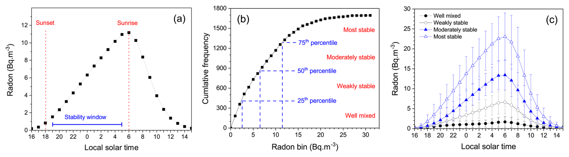
Figure 1 (a) 5 year composite diel radon cycle and averaging window for nocturnal mean radon calculation (advective contributions to the radon signal have been removed; Chambers et al., 2015), (b) cumulative frequency histogram of nocturnal mean radon concentration divided by quartiles representing relative mixing category, and (c) 5 year composite diel hourly radon cycles (±σ) grouped by nocturnal mixing category applied to whole 24 h periods.

Briefly, a nocturnal accumulation window suitable for all seasons (day lengths) is defined (Fig. 1a), the mean radon concentration over this window is calculated each night (referenced to the value at the start of the window to reduce seasonal changes in day length and fetch effects). Nocturnal mean radon concentrations are then ranked each season (since long term average soil moisture changes modify the radon flux and therefore seasonal nocturnal accumulation rates). Strongly negative values represent nights containing significant synoptic non-stationarity or dramatic air mass fetch changes and are removed. Where necessary, Persistent Temperature Inversion (PTI) events can also be identified and removed (Kikaj et al., 2019, 2023). Depending on the application, the remaining nights are then evenly split into 4 or 5 groups (Fig. 1b), covering the range of relative nocturnal stability conditions (from the most well mixed to the most stable) experienced at that site. Each group represents nights with – on average – comparable atmospheric conditions (or meteorological “class types”; see Chambers et al., 2019a, b) and are assigned a “mixing classification”, which is subsequently applied to whole 24 h periods (afternoon to afternoon). Meteorological and trace gas observations composited according to these categories reflect behaviour associated with these conditions (Fig. 1c). The most stable nights exhibit the largest diel amplitudes of concentration changes (due to shallow SNBLs), and well-mixed nights the smallest.

Since the RTM was originally formulated with an assumption of nocturnal stability, and focuses on a comparable nocturnal window, radon-based stability classification can offer an alternative way to apply the RTM that could assist with interpretation of results.

Having removed nights associated with significant synoptic non-stationarity, individual nights within each stability category can be interrogated in the traditional way for suitable radon-to-target gas correlation (R² value) over the defined nocturnal window (e.g. Fig. 2). Since the source functions of target species are typically more spatially heterogeneous than radon's, the range of R² values for each nocturnal stability category in Fig. 2 reflects how similarly distributed the target species emissions were to radon from the contributing fetch on a given night. Nightly regression slopes and associated fetch-appropriate radon fluxes could then be determined, and mean target gas fluxes calculated for each stability category, by month or season.

Since each stability category is associated with a distinct range of nocturnal wind speeds and directions (e.g. synoptic composites in Crawford et al., 2023; Kikaj et al., 2023), they represent a range of contributing fetch regions (decreasing in extent from well-mixed to strongly stable conditions). Contributing fetch regions indicated by a dispersion model, derived only from the selected nights (per month or season) within each stability category, could be used to broadly constrain each contributing fetch. For the more stable nights, when simulated fetch estimates would likely have the largest uncertainty, they could be further constrained using observed wind speed and direction specific to that stability category and observation height.

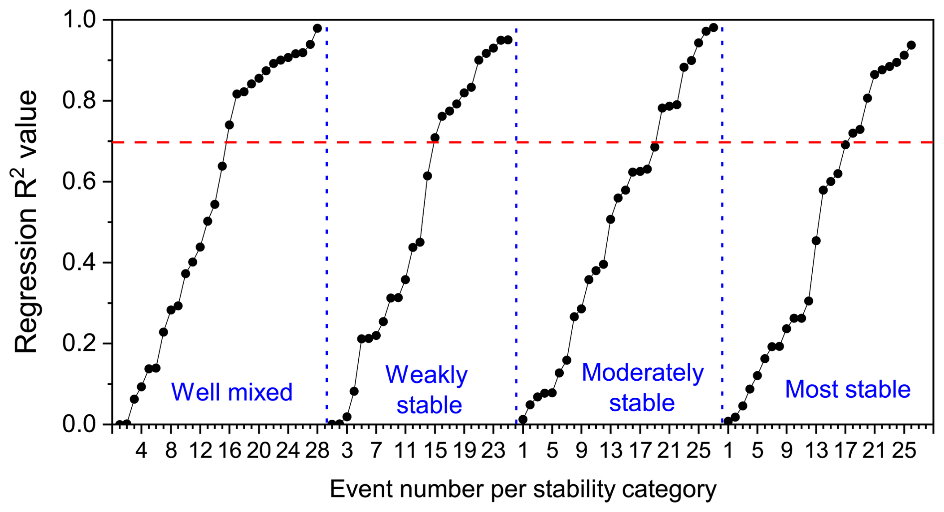
Figure 2 Summer 2022 radon-to-methane regression R² values based on observations at 100 m a.g.l. on the Saclay ICOS tower (ICOS, 2018, 2025; Ramonet et al., 2025) sorted by radon-derived atmospheric mixing category; for reference an R² threshold value of 0.7 has been indicated with a dashed line.

Combining stability classification and the RTM enables estimated fluxes to be more clearly related to specific fetch regions, enables flux estimates for multiple fetch regions to be determined each month/season (rather than just a single estimate), and nights that satisfy the RTM selection criteria within each stability category can be composited prior to performing the radon-to-tracer regression, improving correlations for radon detectors that have a higher measurement uncertainty (see Sect. 3.8). Without using this approach, flux estimates from a potentially wide range of contributing fetch dimensions are irreversibly averaged together, making the result harder to meaningfully interpret.

RTM estimates under the most strongly stable conditions provide emissions estimates at a time when contemporary micrometeorological techniques and ATM inversions fail (Mahrt, 1998; Conen et al., 2002). Furthermore, flagging RTM estimates that occur under less stable conditions provides the ability to more readily compare them with other techniques.

All reported times are Local Solar Time at the respective site.

3 Results

Having outlined the derivation of the RTM, the following sections address considerations for its application and, where relevant, discuss potential flexibility of the underlying assumptions and the impact that relaxing or ignoring these may have on results.

3.1 Defining the nocturnal window

The RTM yields one emission estimate per suitable night. When investigating the co-accumulation of radon and a target species, what is understood to represent “one night” (the accumulation window, AW) will depend on (i) dominant fetch characteristics (e.g. natural, rural, urban), (ii) how conservative the target species is (i.e. spatial and temporal variability of sources/sinks), and (iii) day length. Consequently, the AW needs to be defined on a seasonal and application-specific (i.e. location and measurement height) basis. Throughout the literature AW lengths of 4–13 h have been adopted (e.g. Schmidt et al., 2001; Hammer and Levin, 2009; Levin et al., 2011), though lengths of 8–10 h are more common (e.g. Vogel et al., 2012; van der Laan et al., 2014; Grossi et al., 2018).

As an example, here we compare AW definitions for methane (CH₄) and carbon dioxide (CO₂) at the Cabauw ICOS tower (https://meta.icos-cp.eu/resources/stations/AS_CBW, last access: 29 September 2025), located in a flat, semi-rural setting. To facilitate discussion, we selected only 2 months of data in summer, during which time sunrise was before 06:00 LT and sunset after 21:00 LT.

Diel composite radon at 20 and 200 m above ground level (m a.g.l.) tracked closely between 11:00 and 16:00 LT, indicative of a well-mixed ABL (Fig. 3a). Concentrations at 20 m were higher, consistent with a surface source and no short-term sinks. Concentrations diverged from 17:00 LT, as accumulation began in the SNBL after collapse of the convective boundary layer. Relatively consistent accumulation continued until 05:00 LT, followed by a break in slope as morning convection initiated rapid dilution. The consistency of the 2 month average accumulation, given the variability in summer nocturnal wind directions (typically 170–280°), indicated relatively uniform radon fluxes across the contributing fetch.

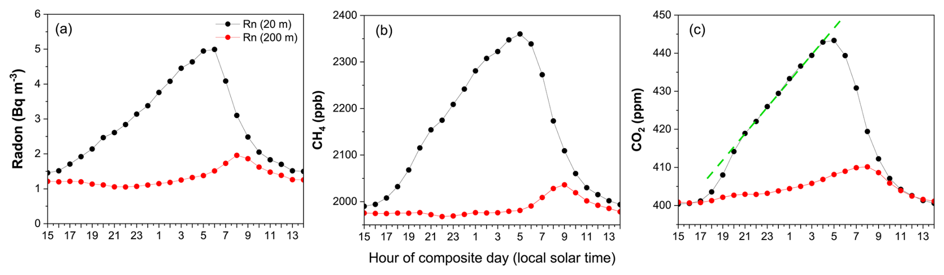
Figure 3 Cabauw 2 month mean diel (a) radon, (b) CH₄, and (c) CO₂ at 20 and 200 m a.g.l. in July and August 2017. Note that diel cycles have been shifted to emphasise nocturnal accumulation (ICOS, 2025; Frumau et al., 2025).

Corresponding CH₄ mixing ratios also tracked closely (Fig. 3b), with higher values at 20 m, indicative of a surface source and few short-term sinks. Its accumulation was less consistent than radon's, suggesting more spatial/temporal variability of sources over the contributing fetch. Unlike radon, between 17:00 LT and sunset (∼ 21:00 LT) the accumulation rate was higher than later in the evening, indicating stronger CH₄ emissions over the contributing fetch.

Corresponding CO₂ mixing ratios (Fig. 3c) demonstrated a balance between photosynthesis, respiration and anthropogenic emissions over the diel cycle. Between 13:00 and 16:00 LT mixing ratios were lower at 20 m, indicative of a net surface sink. In the evening, as mixing decreased, the onset of CO₂ accumulation occurred around 18:00 LT (later than CH₄ due to ongoing photosynthesis). As for CH₄, until sunset a higher rate of CO₂ accumulation was observed than for the rest of the night, suggesting a period of higher CO₂ emissions. Between 21:00 and 04:00 LT CO₂ accumulation was more consistent than for CH₄, indicating a homogeneous source across the contributing fetch. The morning decrease in CO₂ accumulation occurred earlier than for radon or CH₄, because immediately after sunrise there is enough light for photosynthesis but not enough heat to initiate convective mixing.

For maximum radon-to-target gas regression linearity, the source (or sink) characteristics of the target species across the contributing fetch should closely match radon's (i.e. well distributed, relatively consistent). Therefore, for CO₂, all periods when photosynthesis is still active should be excluded. That said, the remaining discussion will focus only on CH₄ AW determination.

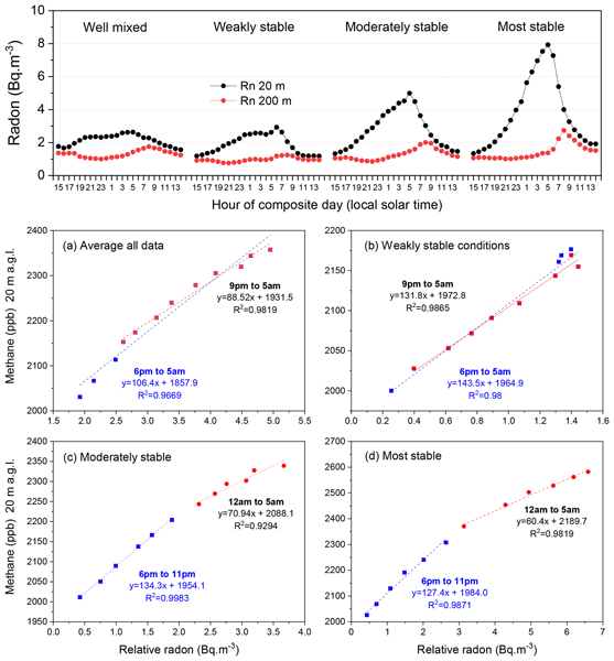
The slope and R² value of the 2 month composite radon-to-CH₄ regression (Fig. 5a) varied with window length (e.g. 18:00–05:00 LT vs. 21:00–05:00 LT, sunset to sunrise). However, this plot represents all data, whereas the RTM was developed for stable conditions. To improve understanding of regression sensitivity to AW length, we assigned radon-based stability categories each night (see Sect. 2.3). Figure 4 depicts diel composites of radon at 20 and 200 m in each of the 4 stability categories: (i) well-mixed, (ii) weakly stable, (iii) moderately stable, and (iv) most stable. Note that these categories are all relative, according to the most and least stable conditions encountered within the limited observation period.

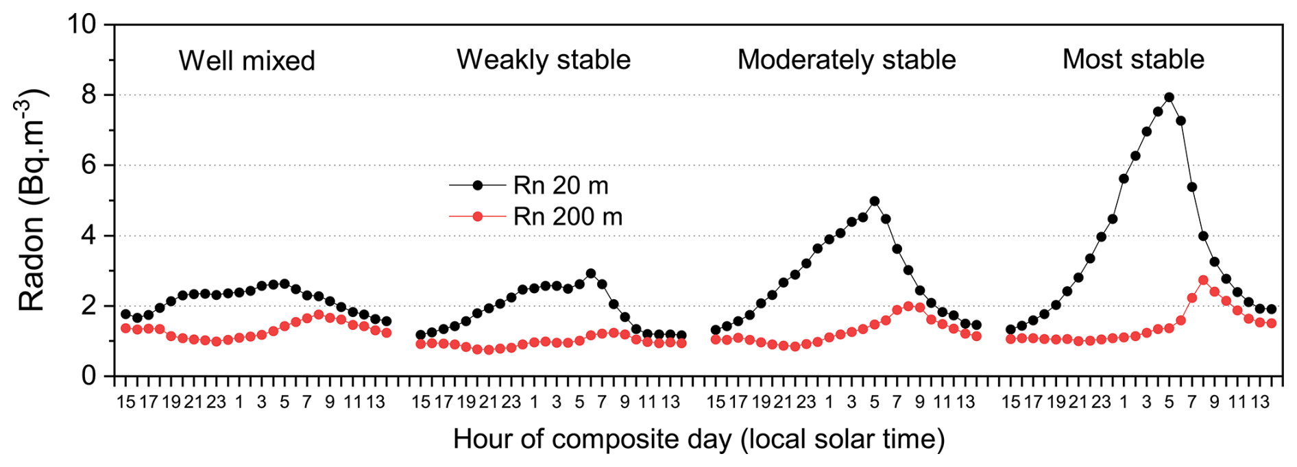
Figure 4 Diel composite hourly mean Cabauw radon at 20 and 200 m associated with 4 radon-derived nocturnal relative stability categories.

Since the RTM traditionally assumes a degree of stability, Fig. 5b–d contrast radon-to-CH₄ regressions on weak, moderate and most stable nights. Weak stability (Fig. 5b) is characterised by moderate wind speeds, frequent cloud cover and relatively deep SNBLs. The diel amplitude of tracers at 20 m was low under these conditions (Fig. 4) and the co-accumulation (radon-to-CH₄ regression; Fig. 5b) relatively linear and consistent throughout the night. Notably the slope was higher than for the 2 month average conditions (Fig. 5a).

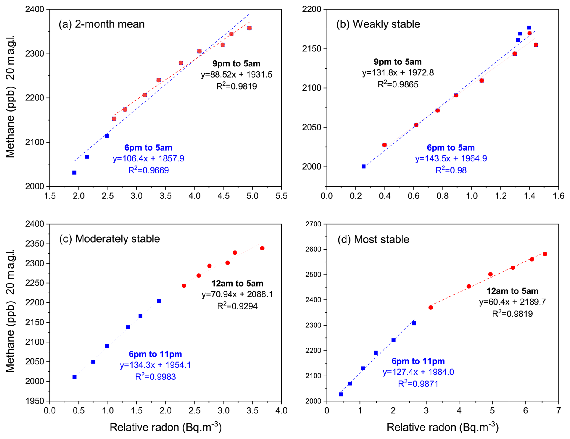
Figure 5 Rn-to-CH₄ regressions of diel composite data between 18:00 and 05:00 LT for (a) all data (the 2 monthly mean), (b) weakly stable nights, (c) moderately stable nights, and (d) most stable nights (ICOS, 2025; Frumau et al., 2025).

By contrast, radon-to-CH₄ regressions for moderate and strong stability (Fig. 5c and d) depicted contrasting accumulation regimes: before and after midnight. Prior to midnight, slopes closely matched those observed under weakly stable conditions (Fig. 5b). After midnight, however, slopes reduced – more so for the stronger stability conditions. To investigate these changes, we analysed wind information from all heights on the tower (Fig. 6).

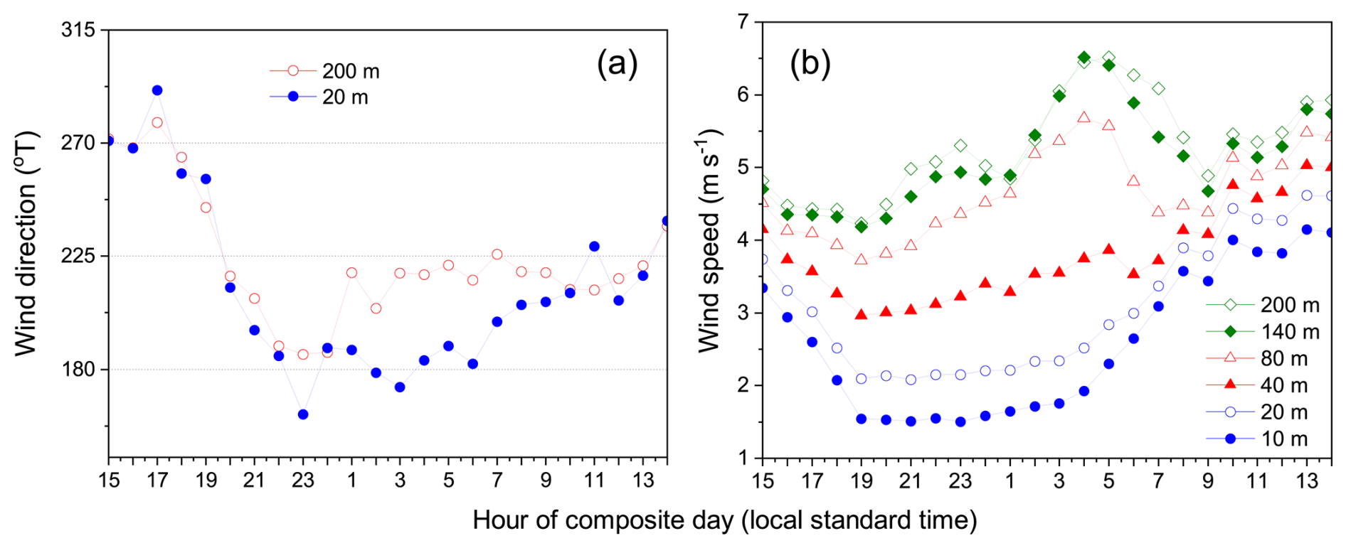
Figure 6 (a) Diel composite hourly wind direction at 20 and 200 m for the most stable nights, and (b) corresponding wind speeds from all available heights (ICOS, 2025; Frumau et al., 2025).

The wind speed profile (Fig. 6b) indicated an inversion height of ∼ 80 $\mathrm{m}\mathrm{a}.\mathrm{g}.\mathrm{l}.$ for the most stable conditions. These nights began with westerly fetch until ∼ 19:00 LT (Fig. 6a; which included urban emissions from The Hague, Fig. B1). Then, until midnight, fetch gradually shifted to the southwest (including urban emissions from Rotterdam and Dordrecht). Between midnight and 05:00 LT, fetch at 200 m was from the southwest, but fetch at 20 m (within the SNBL) was from the south (predominantly rural). Under windier weakly stable conditions (Fig. 5b), there was less difference in wind directions between 20 and 200 m, and fetch was more westerly (220° at 20 m and 230° at 200 m), incorporating emissions from Rotterdam.

Figure 5 demonstrates that combining stability classification with the RTM can not only facilitate AW definition but improve understanding of the contributing fetch. Furthermore, while the temporal resolution of RTM emission estimates is at best monthly, this approach enables emission estimates to be made under different mixing conditions, providing separate monthly estimates for more than one contributing fetch.

These examples demonstrate that AW definition at Cabauw depends on the target fetch (rural or urban). Furthermore, the distinction of results between these fetch types is clearer if stability classification is performed prior to defining the AW length and applying the RTM. Providing monthly or seasonal RTM results without regard to changing stability conditions (e.g. Fig. 5a) mixes emission contributions from various fetch regions in a way that cannot be disentangled, as demonstrated by the distribution of highly correlated radon-to-CH₄ regressions across stability categories in Fig. 2.

Radon-to-CH₄ regression slopes for well-mixed nights (not shown), when winds were moderate-to-strong, directions between 190 and 225° (mixed fetch), conditions typically overcast, and SNBL depths maximised, were associated with a much higher uncertainty of regression fit due to the low diurnal amplitudes of both species and changing fetch characteristics. Consequently, removing the requirement of nocturnal stability when applying the RTM (e.g. Levin et al., 2021), risks significantly increasing uncertainty in the magnitude of RTM fluxes and dimensions of the contributing fetch, and complicating comparisons with bottom-up methods.

Having discussed the nocturnal accumulation window, numerous studies (e.g. Hammer and Levin, 2009; Lallo et al., 2009; Belvisio et al., 2020; Obrist et al., 2005), have applied the RTM to species with distributed sinks (e.g. Hydrogen, Carbonyl Sulfide and Mercury), whose diurnal cycles are characterised by depletion from the SNBL. In determining an appropriate depletion window (DW) in such cases, it is still important that the assumptions of Sect. 2.1 are carefully considered.

In urban environments vehicle emissions are a source of H₂, whereas surface uptake is a sink (Hammer and Levin, 2009). This is evident in Fig. 7a, which compares 2 month (October–November 2023) diurnal composite radon and H₂ measured in Clayton (Victoria, Australia). While typical nocturnal radon accumulation was observed (dawn maximum and late-afternoon minimum), H₂ peaks were observed in the morning and evening, corresponding to periods of simultaneous high traffic density and a developing (or developed) SNBL, reducing the mixing volume. However, in Australian suburbs, traffic density typically reduces to <20 % of peak values between 22:00 and 04:00 LT (e.g. Fig. 4 of Crawford et al., 2016). Under these conditions the surface H₂ sink dominates, and a restricted DW (informed by local traffic density information or katabatic flow characteristics) can be identified within which to apply the RTM to determine local H₂ uptake (Fig. 7b).

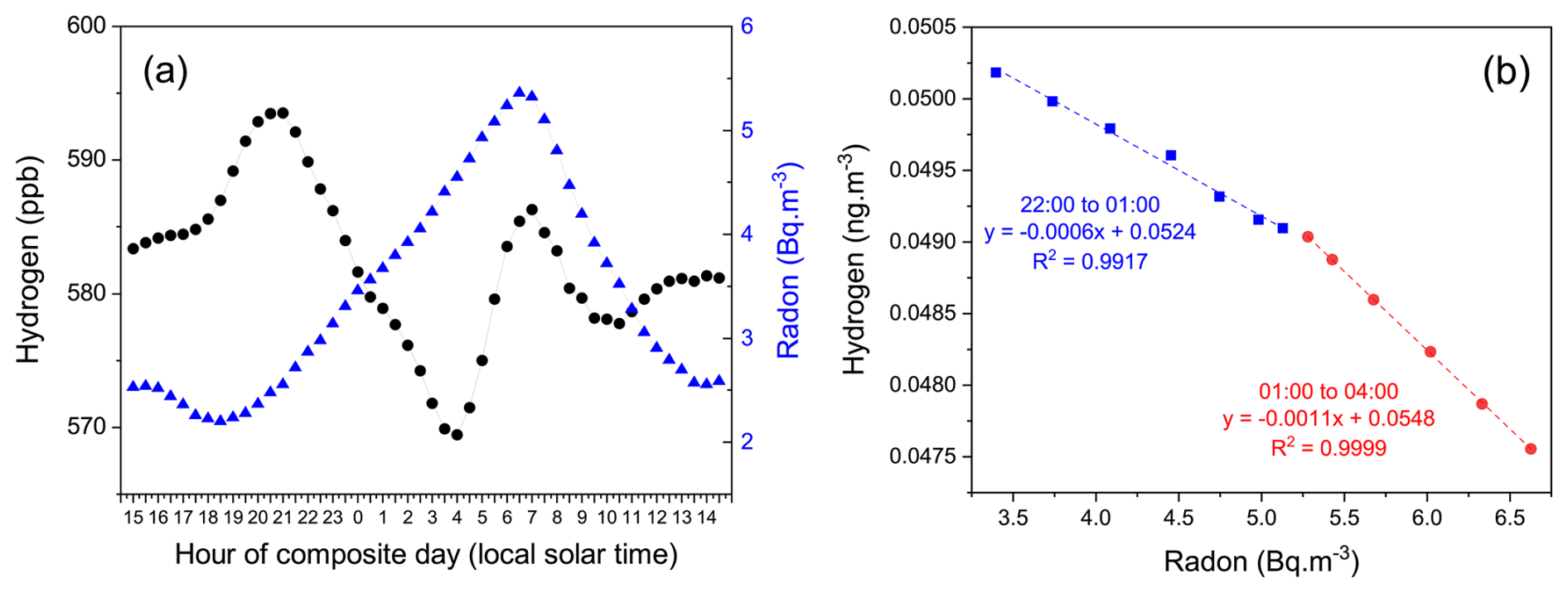
Figure 7 (a) 2 month mean diel radon and H₂ from 20 $\mathrm{m}\mathrm{a}.\mathrm{g}.\mathrm{l}.$ at Clayton (Victoria), in October and November 2024. (b) radon-to-H₂ regressions over the DW 22:00–04:00 LT in two parts. Coastal (south westerly) air masses have been excluded to reduce oceanic influences on radon flux in the contributing fetch.

Assuming a local radon flux of 90 $\mathrm{Bq}{\mathrm{m}}^{-\mathrm{2}}{\mathrm{h}}^{-\mathrm{1}}$ (Griffiths et al., 2010), the average nocturnal H₂ uptake for the October–November period was $-\mathrm{5.4}\times {\mathrm{10}}^{-\mathrm{5}}\mathrm{g}\left({\mathrm{H}}_{\mathrm{2}}\right){\mathrm{m}}^{-\mathrm{2}}{\mathrm{h}}^{-\mathrm{1}}$ from 22:00 until 01:00 LT, and $-\mathrm{9.9}\times {\mathrm{10}}^{-\mathrm{5}}\mathrm{g}\left({\mathrm{H}}_{\mathrm{2}}\right){\mathrm{m}}^{-\mathrm{2}}{\mathrm{h}}^{-\mathrm{1}}$ between 01:00 and 04:00 LT. This change in H₂ uptake corresponded with a shift in fetch from south-southwest to the west-northwest sector that often occurred on stable nights at this site.

This section highlights the importance of case specific determination of the RTM AW, informed by diel characteristics, with careful consideration being given to target gas source/sink characteristics, dominant fetch type, and season.

3.2 Radon and target gas accumulation thresholds

Given the range of sensitivities of radon monitors (e.g. Table 1 of Chambers et al., 2022), and large-scale heterogeneity of radon fluxes (Schery and Wasiolek, 1998; Szegvary et al., 2009; Griffiths et al., 2010; López-Coto et al., 2013; Karstens and Levin, 2024), the signal-to-noise ratio for RTM observations should be carefully considered. This is usually less of a problem in the case of target species (e.g. CO₂, CH₄, N₂O) since the measurement precision of the respective monitors is relatively high (Yver-Kwok et al., 2015).

Historically, radon signal-to-noise ratios for the RTM have been kept in check by: (i) specifying a threshold rate of change over the AW, (ii) specifying a minimum absolute change over the AW, or (iii) requiring a minimum relative change from the well-mixed afternoon ABL value. Generally, ensuring good signal-to-noise ratios also helps satisfy the key assumption for the simplification of Eq. (3) to Eq. (4), that $\mathit{\lambda }{C}_{\mathrm{Rn}}\ll \mathrm{d}{C}_{\mathrm{Rn}}/\mathrm{d}t$.

Levin et al. (2011) recommended a rate-of-change threshold of 3 times the instrument uncertainty. Hammer and Levin, (2009) suggested a 40 % relative increase from afternoon minimum values over the AW. Levin et al. (2021) suggested a radon accumulation threshold equivalent to 50 % of the yearly mean diurnal cycle amplitude at the site.

We use 5 years of radon measurements from a flat, semi-rural site in Australia to put the latter requirement into context. Figure 8a shows the average diel radon cycle, characterised by an afternoon minimum (∼ 2 Bq m⁻³) and near-dawn maximum (∼ 13 Bq m⁻³). According to Levin et al. (2021), to consider applying the RTM at this site, accumulation over the AW (e.g. 18:00–05:00 LT) should exceed $(\mathrm{13}-\mathrm{2})/\mathrm{2}=\mathrm{5.5}\mathrm{Bq}{\mathrm{m}}^{-\mathrm{3}}$ (this value is site specific and depends on sampling height and radon flux). To assess this requirement from an atmospheric stability perspective, the radon-based scheme (see Sect. 2.3) was used to assign nights of the 4 year dataset to relative nocturnal mixing categories (Fig. 8b).

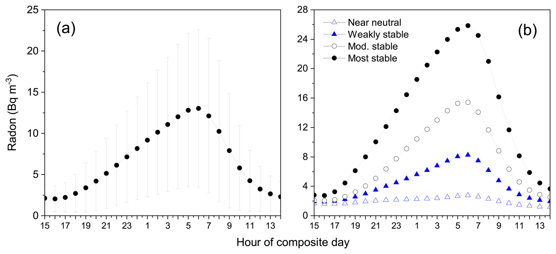
Figure 8 Diel composite (a) overall hourly mean (bars indicate ±1σ), and (b) stability category hourly mean, radon concentrations from 2 $\mathrm{m}\mathrm{a}.\mathrm{g}.\mathrm{l}.$ in Richmond, Australia, over the 4 year period 2007–2011 (adapted from Chambers et al., 2015).

The well-mixed category was characterised by moderate-to-strong winds, frequent cloud cover, and mixing that often extended to the synoptic inversion. Weakly stable, moderately stable, and strongly stable nights each had a thermal inversion between the surface and synoptic inversion. The stronger the stability, the closer the inversion to the surface and the larger the diel radon amplitudes. The criterion of Levin et al. (2021) for applying the RTM therefore equates to at least weakly stable nocturnal conditions. Used in isolation, this is not a strong selection criterion, permitting the use of ∼ 75 % of all nocturnal data. In conjunction with other selection criteria, it is more common for RTM studies focus on only 10 %–15 % of available data (e.g. Hammer and Levin, 2009; Vogel et al., 2012).

A nocturnal inversion isolates processes happening “locally” (beneath that inversion) from influences further afield or above the inversion. Since inversion strength is related to wind speed (and vertical temperature gradient), the spatial extent of “local” influences will scale with inversion strength (see Sect. 3.5). If wind speeds increase sufficiently the inversion will break down (Williams et al., 2013), and the lower atmosphere will mix to the synoptic inversion. In contrast to most prior RTM studies, Levin et al. (2021) argue that nocturnal stability is not strictly necessary for applying the RTM, provided a clear correlation exists between radon and the target species (which frequently occurs, see Fig. 2 “well-mixed”). However, while relaxing the stability constraint increases data availability, as indicated in Fig. 5 it also mixes emission information between very different scales of contributing fetch (10–100 s of kilometres). This may not be advantageous and should be kept in mind when interpreting results or relating fluxes to emission inventories. Relaxing stability constraints also increases the risk of including situations associated with synoptic scale advection (from regions with substantially different fetch characteristics, e.g. near a coastline, Fig. 13), which violates assumptions of the RTM and should be avoided (Vogel et al., 2012). Lastly, without a thermal inversion beneath the synoptic inversion, or other considerations to exclude periods of strong synoptic non-stationarity, a key assumption in deriving Eq. (1) (an impermeable “lid” on the idealised atmospheric column), is no longer guaranteed (i.e. tropospheric air may mix into the ABL, or air from the ABL be vented to the troposphere). Given radon's relatively short half-life, ratios of radon and tracer species in tropospheric air are not likely to be representative of local- to regional-sources.

Adopting an accumulation threshold based on the annual average diel radon cycle would be most successful, and seasonally representative, for regions that do not experience soil freezing and snow cover. The diel radon cycle can be strongly suppressed above frozen and/or snow-covered surfaces through a combination of (i) a reduced radon flux from frozen soils, that can be further reduced by snow cover, and (ii) strongly modified atmospheric mixing due to changes in the surface radiation balance and energy budget:

$$\begin{array}{}\text{(10)}& \begin{array}{rl}& \left(S_{\text{IN}}-S_{\text{OUT}}\right)+\left(L_{\text{IN}}-L_{\text{OUT}}\right)=R_{\text{NET}}\\ & =H+LE+G+\mathrm{\Delta }S,\end{array}\end{array}$$

where $S_{\text{IN}}/S_{\text{OUT}}$ are incoming and outgoing shortwave radiation, $L_{\text{IN}}/L_{\text{OUT}}$ are incoming and outgoing longwave radiation, R_NET is the net radiation remaining at the surface to be redistributed, H is the sensible heat flux (which drives convection), LE the latent heat flux (evapotranspiration), G the ground heat flux, and ΔS transient energy storage in the canopy layer.

Snow increases reflectivity (albedo), reducing available R_NET for partitioning into H, LE, G and ΔS. Furthermore, a greater proportion of remaining R_NET is partitioned into G and LE, reducing the potential for convective mixing. Combined with the increased likelihood of winter cloud cover in such regions (Górowski et al., 2025), these factors result in a reduced contrast in day/night atmospheric mixing depth. Consequently, near-surface winter diel radon cycles can be reduced to 30 %–50 % of the amplitude observed in other seasons (Williams et al., 2016; Chambers et al., 2016a; Kikaj et al., 2023), making it difficult to find appropriate nights to apply the RTM (Vogel et al., 2012). In fact, applying an annual mean accumulation threshold equally to the whole year could result in winter months being completely excluded from analyses. For this reason, given sufficiently sensitive radon measurements (see Sect. 3.8), nocturnal accumulation thresholds should be determined and applied seasonally. In this situation, radon-based stability classification in winter – focussing on only the most strongly stable non-PTI conditions – may provide the best opportunity to successfully apply the RTM and achieve the most accurate results.

Diel radon cycles can be further suppressed during PTI conditions, often observed across Europe (and parts of the central west USA) in winter and autumn due to persistent large-scale subsidence events (e.g. the “Siberian High”; Kikaj et al., 2019, 2023; Baasandorj et al., 2017). Under such conditions, radon and surface emitted pollutants, can accumulate under the larger-scale subsidence inversion for periods of days to weeks, because combined changes in the radiation budget and surface energy balance don't allow sufficient daytime convective heating to break through the subsidence inversion and disperse the accumulated pollution. Meanwhile, a supressed diurnal variability (superimposed on higher, and growing, background concentrations) can also be observed, driven by the development of weaker nocturnal surface inversions within the subsidence inversion. Such conditions should be avoided for RTM applications.

3.3 Radon-to-target gas regression linearity threshold

An underlying assumption of the RTM (Sect. 2.1) is that source functions of radon and target species should be broadly distributed and relatively homogeneous. If these conditions are met over the contributing fetch their co-accumulation will be linearly correlated. Many conditions can lead to non-linearity, including differences in source distributions, differences in temporal variability of the source functions, changes in the contributing fetch, the existence of point sources, or higher chemical reactivity of the target species over SNBL mixing timescales or length of the AW.

The linearity of the radon-to-target regression is therefore a useful measure of how well the necessary assumptions of the technique are being met. In general, when sampling within the SNBL, the stronger the nocturnal stability, the smaller the contributing fetch region. For distributed sources, the smaller the fetch region (10 s rather than 100 s of kilometres), the higher the probability that fluxes of both species will be near-homogeneous over this area, resulting in larger R² values.

Some early applications of the RTM adopted R²≥0.5 as a minimum requirement (e.g. Levin et al., 1999), but contemporary studies have typically required R² to be larger than 0.6–0.8 (Vogel et al., 2012; Grossi et al., 2018; Levin et al., 2021). When assessing the correlation between the two species it is important to employ a regression algorithm that accounts for uncertainties in both x and y coordinates (Yver-Kwok et al., 2025). Imposing a threshold of R²≥0.8 typically results in ≥80 % of observations being rejected (see Fig. 2) but will yield a dataset that most closely satisfies the assumptions of the technique.

Levin et al. (2021) demonstrated that moderate heterogeneity within the contributing fetch (i.e. excluding strong point sources or step changes in source function characteristics) can be accommodated by the RTM if (i) the heterogeneity is at small spatial scales relative to the contributing fetch and randomly distributed, and (ii) is not correlated with atmospheric transport processes acting on short temporal and spatial scales. Isolated instances of flux heterogeneity (e.g. brief influence of a point source) or temporal flux variability will present as an outlier from the dominant linear trend (Hammer and Levin, 2009; Vogel et al., 2012). For longer accumulation windows (e.g. 7–10 h), if only a few samples each night are impacted they can be excluded from the regression, so long as at least 80 % of the nocturnal window data is retained for the regression analysis (Levin et al., 2011). If less than 5 hourly observations can be retained for analysis (or 4 h of 30 min observations), consider rejecting the whole night.

Step changes in flux characteristics within the contributing fetch (e.g. coastlines) should be avoided. A fundamental assumption of the RTM is that the rate of accumulation observed for both species is a function of only (i) a (relatively) constant flux over the contributing fetch, and (ii) the changing nocturnal mixing depth. Compared with terrestrial surfaces, most open water bodies are characterised by near zero emissions of radon or target species. If a contributing fetch includes a coastline, the observed accumulation can then also become a function of wind direction and wind speed, which are unlikely to remain constant over an entire AW. For sites near coastlines, the more relaxed the nocturnal stability criteria, the more likely this is to be a problem.

Prior to assessing the regression linearity, temporal discrepancies between the radon and target gas observations need to be accounted for. If measuring radon with an ANSTO two-filter dual flow-loop monitor the appropriate response time correction must be applied (Griffiths et al., 2016), or slope errors of up to 6 % can result due to the instrument's 45 min response time. Temporal discrepancies of other kinds can be determined by performing a cross correlation between the observed quantities and adjusting the timestamp of the least well-defined measurement to maximise the absolute correlation.

Furthermore, if developing a fitting algorithm, as well as having the ability to identify and exclude outliers, it should also look several hours beyond the AW (Vogel et al., 2012). If measuring close to the surface (e.g. $\le \mathrm{25}\mathrm{m}\mathrm{a}.\mathrm{g}.\mathrm{l}.$, as in Vogel et al., 2012) a linear correlation persists beyond the AW (i.e. after the onset of morning convection is expected for that season), it is likely associated with a synoptic event (e.g. distant advection from a region of contrasting flux characteristics (e.g. Fig. 13), or the development of a PTI), and the data should be excluded. When measuring from taller towers (e.g. 50 to 200 $\mathrm{m}\mathrm{a}.\mathrm{g}.\mathrm{l}.$), however, near-linear correlations can persist several hours after sunrise as near-surface air with higher trace gas concentrations is mixed within (or into) the growing convective boundary layer.

Finally, assuming the RTM has been applied under optimal conditions (within the SNBL under strongly stable conditions), it will typically underestimate emissions if point sources exist in the contributing fetch (Levin et al., 2021). This can occur because mixing within the SNBL is not homogeneous, or because the point sources may be emitted directly into the residual layer (above the inversion) via tall stacks. However, Levin et al. (2021) make the point that emission characteristics of large point sources (e.g. industry) are usually quite well known and can be included retrospectively. Typically, it is the more distributed natural and anthropogenic sources that are less well constrained, and these are ideally suited to characterisation by the RTM (Vogel et al., 2012). If combining stability classification with RTM, well-mixed to moderate stability classes are more likely to include influences of point sources in the contributing fetch, since the associated nocturnal mixing depths are deeper and wind speeds higher than for the most stable conditions.

3.4 Measurement height

The RTM was originally formulated by considering the co-accumulation of surface emitted species in a SNBL of depth H^′, a theoretical mixing length scale representing the height to which surface emissions are assumed to uniformly mix (see Eqs. 1 and 2). An example of how H^′ varies with relative nocturnal stability over a flat, predominantly rural floodplain site is provided in Fig. 9. Here we applied the box model of Griffiths et al. (2013) to 5 years of observations previously described by Chambers et al. (2015) (see also Sect. 3.2). The average H^′ each night was calculated using the last 5 h before dawn. Nightly mean H^′ were subsequently grouped by stability category.

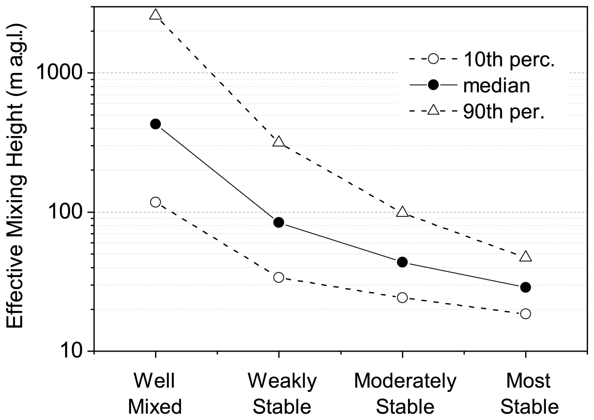
Figure 9 Distributions (10th/50th/90th percentile) of nocturnal mean equivalent mixing heights within 4 mixing categories over a flat, semi-rural site in Richmond, Australia, based on 5 years of observations (note logarithmic y-axis). The site is characterised by mixed crops, pasture, scattered low trees and small, isolated single-storey structures.

For homogeneous agricultural land, or sparsely vegetated surfaces, expected H^′ values would be lower than depicted in Fig. 9, whereas over tall, heterogeneous forest canopies, urban regions or undulating terrain, the expected corresponding H^′ could be higher. Of interest to note in Fig. 9 is that for around 25 % of near-neutral nights, characterised by moderate to strong winds and frequent overcast conditions, the lower nocturnal atmosphere appeared fully mixed through to the synoptic inversion (i.e. no residual layer).

For conditions of moderate- to strong-stability over flat, semi-rural fetch, H^′ was typically below 100 m (Fig. 9). Furthermore, H^′ was also <100 m for most weakly stable nights. Consequently, careful consideration should be given to fetch characteristics before applying the RTM at tall tower sites (e.g. European ICOS network towers, typically 100–200 m tall). To demonstrate, we briefly discuss several examples of ICOS station measurements, from Cabauw (the Netherlands), Trainou (France) and Saclay (France).

Radon diel cycles at Cabauw (Fig. 4) exhibit little nocturnal accumulation at 200 m, indicating this sampling height is usually above the SNBL for weakly through strongly stable conditions. Similarly, monthly mean radon diel cycles from 180 m on the Trainou ICOS tower (Fig. 11, Pal et al., 2015), show little nocturnal radon accumulation ($<\mathrm{1}\mathrm{Bq}{\mathrm{m}}^{-\mathrm{3}}$), followed by radon peaks several hours after sunrise, as would be expected following the convective breakdown of a morning inversion that had formed below the sampling height. In contrast to Lopez et al. (2012) who reported that the 180 m Trainou measurements are within the SNBL around 50 % of the time, regardless of season, the results of Pal et al. (2015) suggest that the 180 m measurements at Trainou are not often within the SNBL.

By contrast, Fig. 10 depicts diel composite radon at 15 and 100 m on the Saclay ICOS tower, grouped by stability category (Sect. 2.3). The local fetch for this tower has undulating terrain, covered by a mixture of forests, agricultural and semi-urban regions (Yver-Kwok et al., 2025). Further afield (north through east) is the Paris urban agglomeration. For weak to strong stability conditions a nocturnal accumulation of 2–3 Bq m⁻³ is evident at 100 m, with peak values occurring after sunrise when higher radon concentrations from lower in the SNBL are mixed upwards by convection. Clearly the 100 m Saclay measurements are often within the SNBL. Of note, accumulation rates are more uniform at 100 m, but accumulation magnitude is 2–3 times higher at 15 m (highlighting the non-uniformity of mixing within the SNBL, Sect. 2.2).

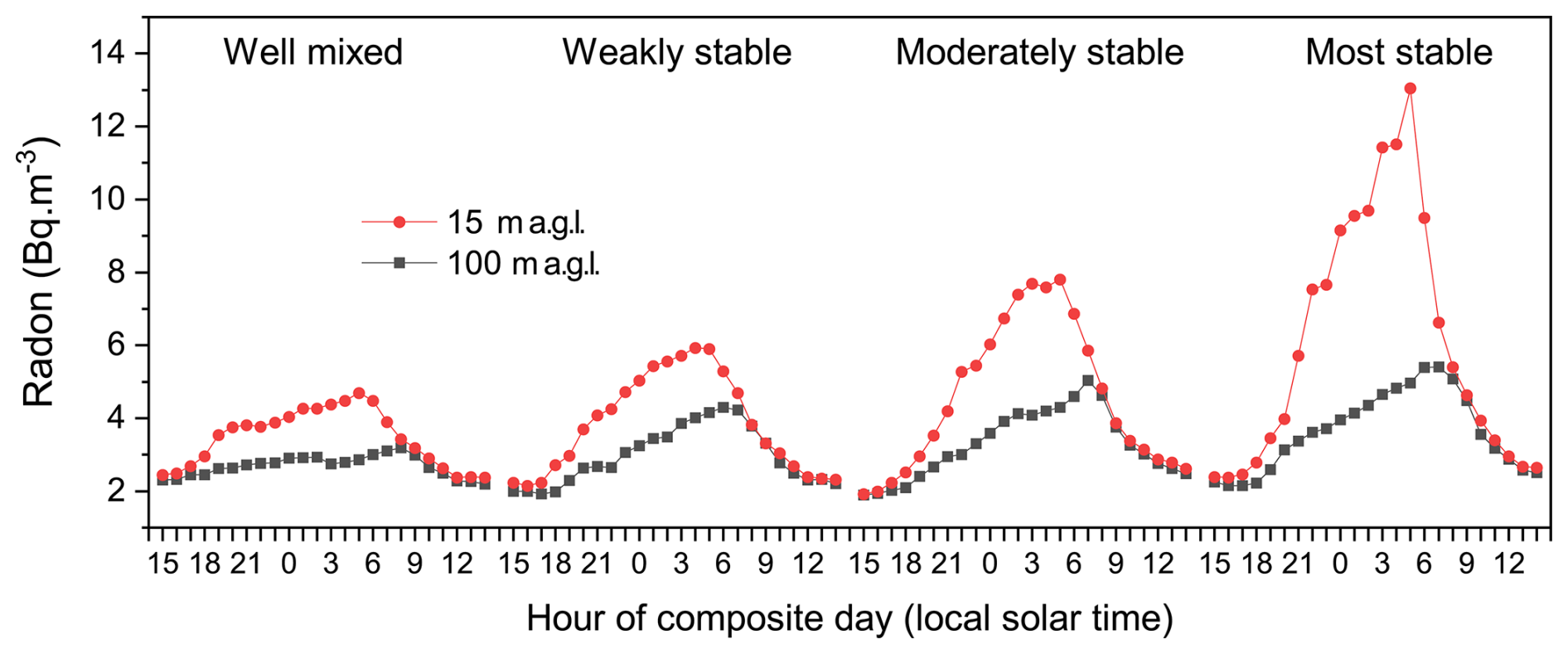
Figure 10 Diel composite radon concentrations as a function of nocturnal mixing category at 15 and 100 m on the Saclay ICOS tower, France, between June and September 2022 (ICOS, 2018, 2025).

When Saclay CH₄ observations were grouped by the same stability categories (Fig. 11), while accumulation under the most stable conditions were clearly discernible at both heights, the other categories were much less distinct. This evident contrast between radon and CH₄ is attributable to two main factors: (i) a larger spatial variability in the CH₄ source function than for radon, and (ii) a tendency for different nocturnal stability regimes to experience very distinct contributing fetch regions due to contrasting synoptic meteorology conditions (Crawford et al., 2023; Kikaj et al., 2023).

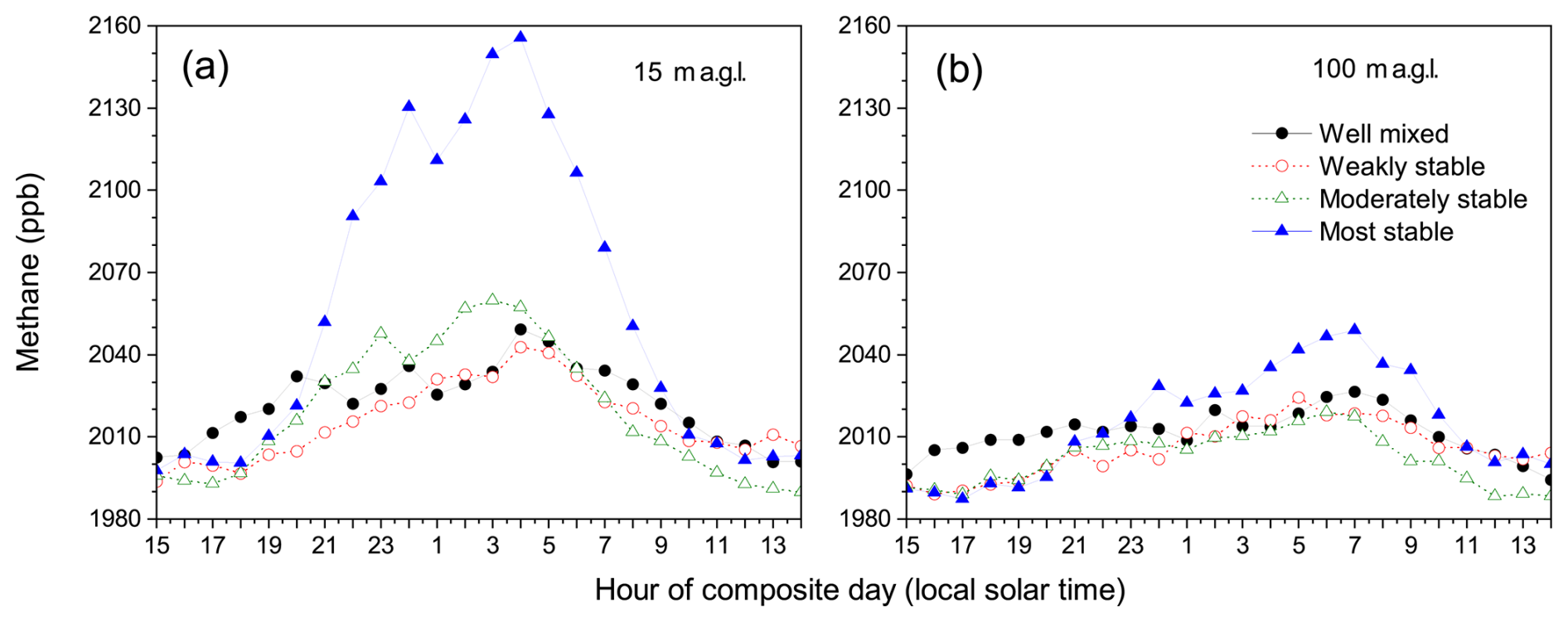
Figure 11 Corresponding diel composite CH₄ mixing ratios at (a) 15 $\mathrm{m}\mathrm{a}.\mathrm{g}.\mathrm{l}.$ and (b) 100 $\mathrm{m}\mathrm{a}.\mathrm{g}.\mathrm{l}.$ on the Saclay ICOS tower for the mixing categories shown in Fig. 10 (ICOS, 2018, 2025; Ramonet et al., 2025).

Figure 12a and b depict Rn-to-CH₄ regressions between 19:00 and 05:00 LT based on composites of all strongly stable summer nights. Figure 12c and d depict corresponding plots for only the strongly stable nights with R²>0.7 (refer to Fig. 2). Two things are evident from these plots: (i) the composite based on all stable nights is better suited to define the AW for this site and stability regime (since it is more statistically sound), and (ii) regression slopes are notably larger when only the R²>0.7 nights are selected (Fig. 12c and d).

At both heights on the Saclay tower there were two accumulation regimes evident under strongly stable conditions: before and after 22:00 LT (Fig. 12a and b). Based on these results, we selected a 22:00–05:00 LT AW (indicated by red markers) for RTM flux estimates.

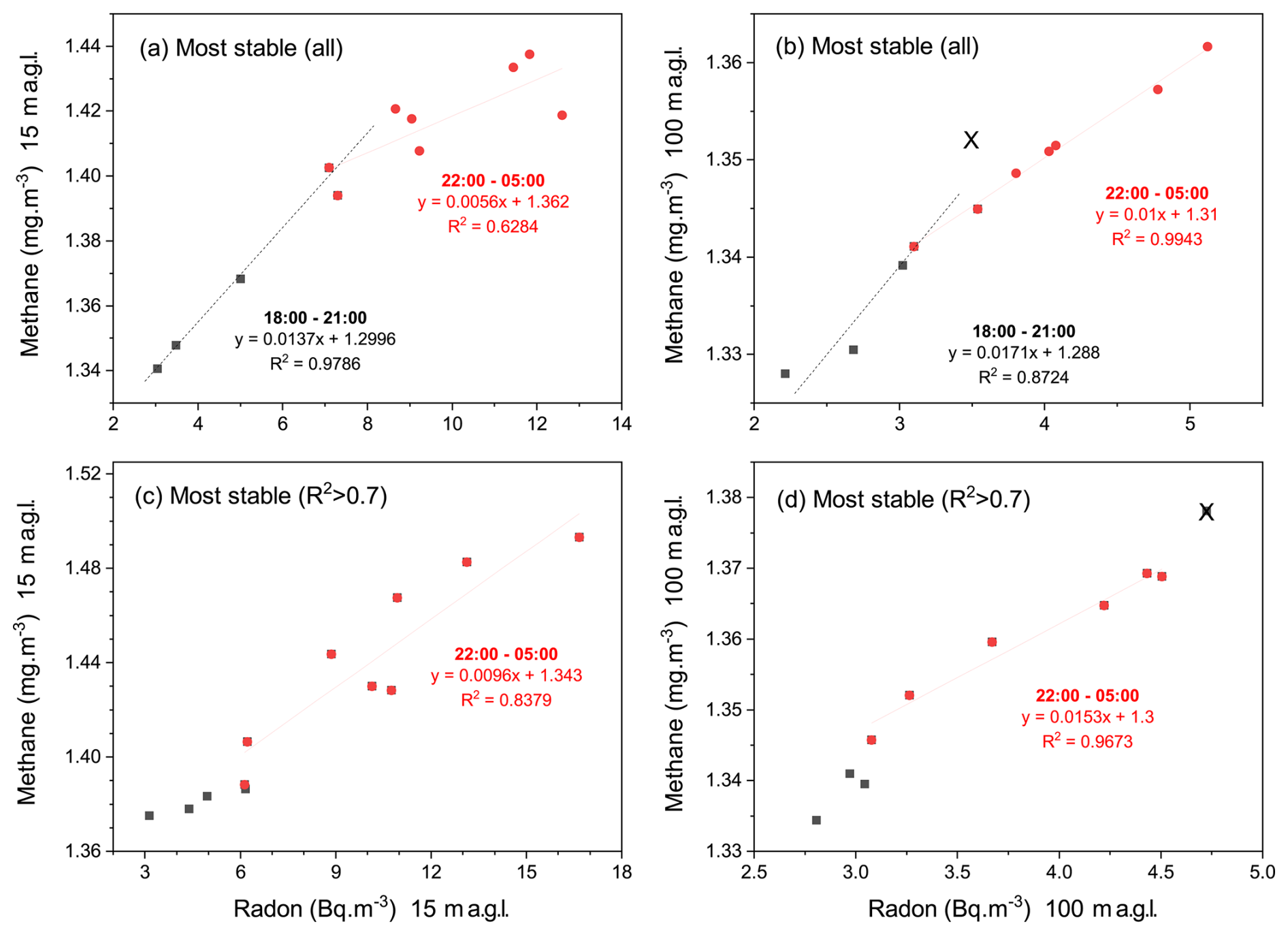
Figure 12 Rn-to-CH₄ regressions at 15 and 100 m at Saclay for the most stable nights. One marked outlier marked with a cross was excluded from the regressions of (b) and (d) (ICOS, 2025; Ramonet et al., 2025).

For the following summertime Saclay CH₄ flux estimates we calculated Rn-to-CH₄ regression slopes in 3 ways: (1) the average slope for all nights with R²>0.7 in each stability category; (2) as for (1) but up to 2 outliers from the 8 hourly samples in the AW were removed from individual nightly regressions such that each R²>0.9; and (3) a single slope derived from a Rn-to-CH₄ regression calculated from hourly composite radon and CH₄ values for nights in each category where R²>0.7.

CH₄ flux estimates in Table 1 were calculated by scaling the regression slopes by 0.965 to account for nocturnal radon decay (see Sect. 2.1), then multiplying by a representative summer radon flux for the tower's contributing fetch. The annual average radon flux for this region is 52 $\mathrm{Bq}{\mathrm{m}}^{-\mathrm{2}}{\mathrm{h}}^{-\mathrm{1}}$ (Yver-Kwok et al., 2024). However, as noted by Levin et al. (2021), it is not unusual to see a soil moisture-driven seasonality in radon flux of order ±25 %–30 %. This is in good agreement with the seasonal changes in radon flux from the Saclay contributing fetch reported by Yver-Kwok et al. (2024; their Fig. 7), from which we assumed a representative summer radon flux of 70 $\mathrm{Bq}{\mathrm{m}}^{-\mathrm{2}}{\mathrm{h}}^{-\mathrm{1}}$.

Table 1 Summer RTM-based CH₄ flux estimates [$\mathrm{mg}\left({\mathrm{CH}}_{\mathrm{4}}\right){\mathrm{m}}^{-\mathrm{2}}{\mathrm{h}}^{-\mathrm{1}}$] from 15 and 100 $\mathrm{m}\mathrm{a}.\mathrm{g}.\mathrm{l}.$ observations on the Saclay ICOS tower (see text for explanation of the three estimates).

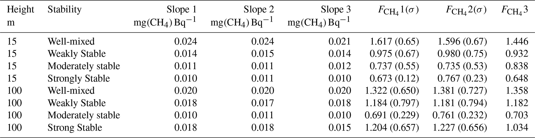
Focussing discussion on method 2 above (the most similar to existing RTM applications), CH₄ flux estimates from both heights were larger under well-mixed conditions than under strongly stable conditions. This is consistent with higher wind speeds (larger contributing fetch) under well mixed conditions, and wind directions at this site in summer often coming from the Paris urban agglomeration (Yver-Kwok et al., 2025). In the direction of Paris, the initial ∼ 10 km of fetch is dominated by forests and agriculture. Furthermore, fluxes estimated from the 15 m observations (with the reduced contributing fetch) were generally smaller than those estimated from 100 m. At 100 m, under strongly stable conditions, estimated CH₄ fluxes were higher than for weak to moderate stability conditions. This may be because the AW under strongly stable conditions should have been shorter (e.g. 23:00–05:00 LT instead of 22:00–05:00 LT, see Fig. 12d), or because potentially the 100 m sampling height may not have been completely within the SNBL for the whole of each night.

Under well-mixed conditions, estimated CH₄ emission from the contributing fetch (including the Paris region) was 1.4 ± 0.73 to 1.6 ± 0.67 $\mathrm{mg}\left({\mathrm{CH}}_{\mathrm{4}}\right){\mathrm{m}}^{-\mathrm{2}}{\mathrm{h}}^{-\mathrm{1}}$, while emissions under the most stable conditions (representing more of the nearby forested/agricultural regions and less of Paris) was 0.77 ± 0.23 to 1.23 ± 0.66 $\mathrm{mg}\left({\mathrm{CH}}_{\mathrm{4}}\right){\mathrm{m}}^{-\mathrm{2}}{\mathrm{h}}^{-\mathrm{1}}$. By comparison, Fig. 10 of Yver-Kwok et al. (2024) show summertime 100 m RTM CH₄ fluxes for this site in 2022 to vary between 0.2–2.3 $\mathrm{mg}\left({\mathrm{CH}}_{\mathrm{4}}\right){\mathrm{m}}^{-\mathrm{2}}{\mathrm{h}}^{-\mathrm{1}}$, with average values ∼ 0.95 $\mathrm{mg}\left({\mathrm{CH}}_{\mathrm{4}}\right){\mathrm{m}}^{-\mathrm{2}}{\mathrm{h}}^{-\mathrm{1}}$. While, overall, the results are quite similar between these two studies, the inclusion of radon-based stability classification allows a clearer distinction between contributing fetch regions. The June–September 2022 average CH₄ flux from all sources for the Saclay region based on EDGAR v8.1 (Crippa et al., 2024) emissions was 0.86 $\mathrm{mg}\left({\mathrm{CH}}_{\mathrm{4}}\right){\mathrm{m}}^{-\mathrm{2}}{\mathrm{h}}^{-\mathrm{1}}$; lower than the estimate from this and the Yver-Kwok et al. (2024) study.

A number of corollaries arise from the ICOS tower case studies above: (i) the accumulation signal-to-noise ratio improves under stable conditions compared with well-mixed conditions, and the stronger the stability the better (within the SNBL), (ii) unless an ICOS tower is situated over a tall forest canopy, undulating terrain, or an urban region, measurements from >100 m would likely only observe nocturnal accumulation during a limited number of weakly stable evenings each month, (iii) signal-to-noise ratios improve the nearer measurements are to the surface in the SNBL but the effects of heterogeneity on accumulation are increased, (iv) for a given measurement height the stronger the stability conditions, the more local the contributing fetch, and (iv) the lower the measurements within a SNBL the more local the contributing fetch region, so the choice of sampling height should be made with a contributing fetch scale in mind (see Sect. 3.5).

Generally, measurement heights ≥ 30 $\mathrm{m}\mathrm{a}.\mathrm{g}.\mathrm{l}.$ are better suited for characterising integrated fluxes from regional-scale (hundreds of kilometres) than local-scale (tens of kilometres) fetch regions. If sampling is only possible from measurement heights near the inversion or above the SNBL, the idea of applying the RTM with a view to studying truly “local” fetch regions (radius of tens of kilometres) should be abandoned. For larger contributing fetch regions, other implementations of the RTM can also be explored (see Sect. 1).

Levin et al. (2021) suggested removing the RTM nocturnal stability criteria (or even sampling within the residual layer). While the radon-to-tracer ratios under such conditions are still representative of recent surface–atmosphere exchange processes, the contributing fetch regions become extremely large and poorly constrained, and the small diel signal amplitudes under well-mixed conditions (see Figs. 4 and 10) could lead to accumulation rates below instrument detection limits, increasing measurement uncertainty.

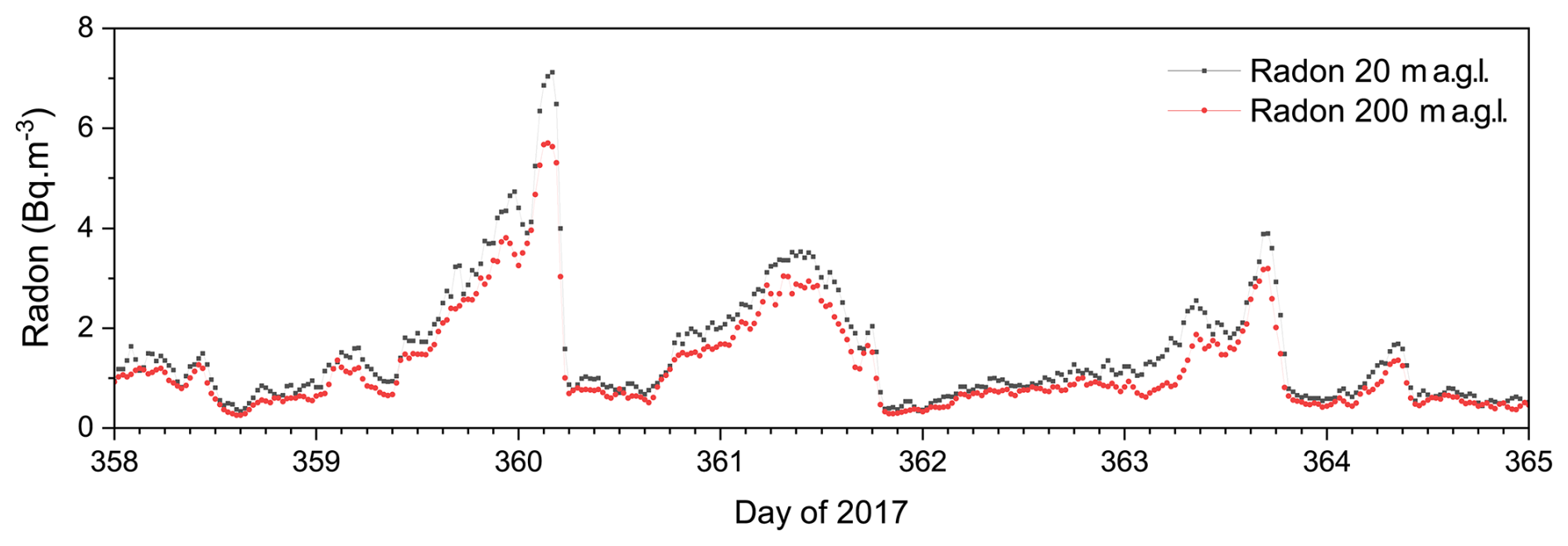
Figure 13 1 week of radon observations from the Cabauw ICOS tower in December 2017, indicating several transitions related to synoptic changes in air mass fetch that are independent of diurnal mixing variability.

Related to the above, in the absence of a nocturnal stability criterion (or related wind speed threshold), more care is required to exclude influences of synoptic processes if automated scripts are being used to apply the RTM. Under conditions of moderate to strong winds, air mass “time over land” (rather than changing nocturnal mixing depth) can cause co-accumulation of radon and other trace species within the boundary layer over greater than diel timescales, and this accumulation can be “reset” by sudden changes in wind direction to recent oceanic fetch. Figure 13 shows several such examples from December 2017 observed at the Cabauw ICOS tower, which is ∼ 40 km from the North Sea coast. Several fetch-driven periods of accumulation are evident, each with rapid transitions back to recent oceanic fetch. Radon and CH₄ were positively correlated (with high R²-values) throughout both the accumulation and reset periods, with the characteristics of these events (magnitude and duration) varying with wind speed and direction. As evident from this example, it is not uncommon for such events to happen within or across the AW, so they need to be identified and excluded for which software solutions have been developed (Levin et al., 1999; Hammer and Levin, 2009; Vogel et al., 2012). Alternatively, imposing a requirement of strong atmospheric stability for the RTM (and/or potentially reducing the measurement height) would enable the technique to be used within ∼ 15 km of a coastline without actively having to exclude wind sectors that include nearby coastlines.

While formulation of the RTM in Sect. 2.1 assumed uniform mixing of tracers within the atmospheric column, in a stably stratified atmosphere tracers with surface sources usually exhibit strong vertical gradients (e.g. Fig. 14a; see also examples in Table 1 of Chambers et al., 2011). Consequently, when using the RTM for species that can exhibit low amplitude diurnal cycles (e.g. N₂O), unless measuring under strongly stable conditions, within the lower half of the SNBL, rates of change within the AW can at times approach the instrument's detection limits. Consequently, for measurements over simple, low canopies (e.g. pasture, crops, semi-rural regions) a suitable height for measurements intended for local RTM applications should be $<\mathrm{30}\mathrm{m}\mathrm{a}.\mathrm{g}.\mathrm{l}.$. Indeed, many applications of the RTM have focussed on measurement heights between 7 and 25 $\mathrm{m}\mathrm{a}.\mathrm{g}.\mathrm{l}.$ (Lopez et al., 2012; Vogel et al., 2012; Belvisio et al., 2013; Grossi et al., 2018), remaining within the SNBL, while not limiting potential fetch regions to very local.

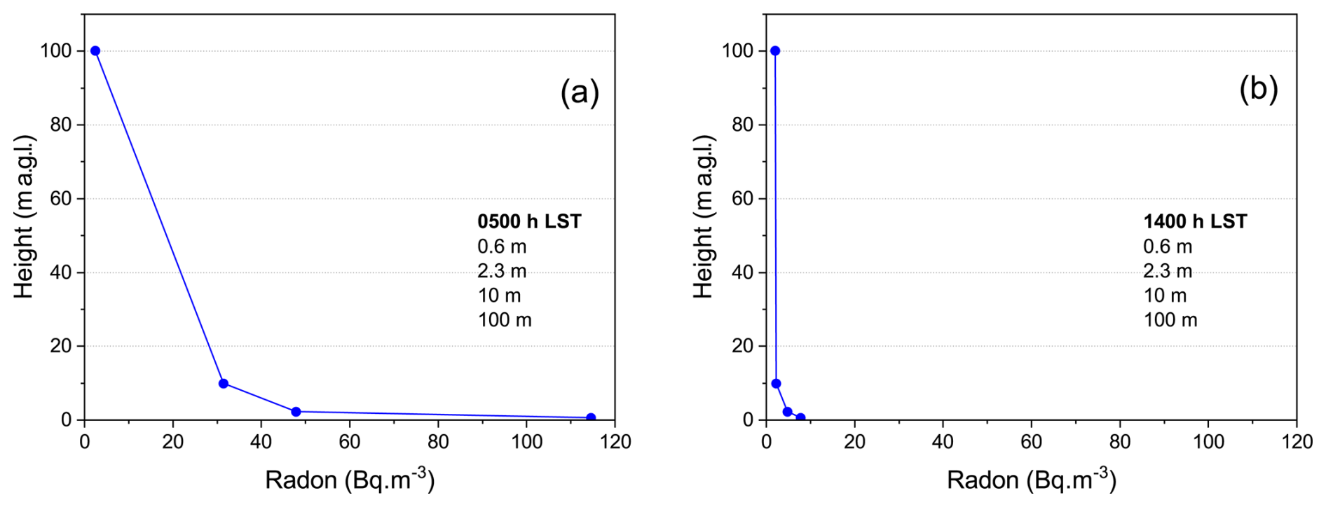
Figure 14 Radon measurements at 0.58, 2.34 and 10 m (from a tower) and ∼ 100 m from a light aircraft, in Goulburn, Australia, November 2011 (a) just pre-dawn, and (b) in the early afternoon.

When measuring above undulating terrain, forest canopies, or suburban/urban environments, however, appropriate measurement heights and data selection criteria will need to be assessed on a case-by-case basis. Levin et al. (1999, 2021), for example, measured within Heidelberg city near the peak urban canopy height (30 m–40 $\mathrm{m}\mathrm{a}.\mathrm{g}.\mathrm{l}.$).

Another assumption of the RTM is that both species are acted upon by the same transport and mixing processes. This requirement is most easily satisfied by making measurements at the same height and location. Notably, some applications of the RTM in the literature have not strictly adhered to this recommendation (e.g. Lopez et al., 2012; Belviso et al., 2013, 2020; when observations were being made between 2 and 15 $\mathrm{m}\mathrm{a}.\mathrm{g}.\mathrm{l}.$). The closer the measurements are made to the surface, and the stronger the stability, the more important co-location becomes (e.g. Fig. 14a). For well-mixed through weakly-stable conditions, when turbulence is vertically more continuous and better connected to the surface, mixing length scales increase with distance from the surface. Consequently, the further removed measurements are from the surface, the less a small difference in measurement height and spatial location will impact the results. Under very stable conditions however, the flow becomes strongly stratified (e.g. Fig. 14a), mixing becomes intermittent, and localised flow patterns can develop (Williams et al., 2013). Under these conditions measuring at the same height and location becomes critical to satisfy the assumption that both gases are being acted upon by the same processes.

In the case of forest canopies nocturnal mixing depths will depend on the roughness “seen” by the atmosphere, which is different for closed vs. open canopies, or broadleaf vs. coniferous canopies. As an example, Fig. 15 depicts diel composite CO₂ mixing ratios made within and above an 18 m coniferous forest in Hyytiälä, Finland, in the growing season. Composites were assigned mixing categories as described in Sect. 2.3 based on radon measurements made within the canopy at 6 $\mathrm{m}\mathrm{a}.\mathrm{g}.\mathrm{l}.$ (using the method of Paatero et al., 1994); only the mixing extremes (well-mixed and most stable cases) are shown. Compared with the well-mixed conditions, nocturnal CO₂ accumulation was observed under the most stable nocturnal conditions at this site up to ∼ 50 m above the mean canopy height. If applying the RTM to regions with dense forest canopies, particularly for species such as CO₂ which has nocturnal sources both at the surface and throughout the canopy, the version of Eq. (5) suggested by Martens et al. (2004) employs differences between canopy profile mean concentrations and the corresponding SNBL value (i.e. $\mathrm{\Delta }{\mathrm{CO}}_{\mathrm{2}}={\mathrm{CO}}_{\mathrm{2}\mathrm{\_}\mathrm{CP}}-{\mathrm{CO}}_{\mathrm{2}\mathrm{\_}\mathrm{SNBL}}$, where CO_{2_CP} is the mean canopy profile CO₂ and CO_{2_SNBL} is CO₂ measured above the canopy within the SNBL).

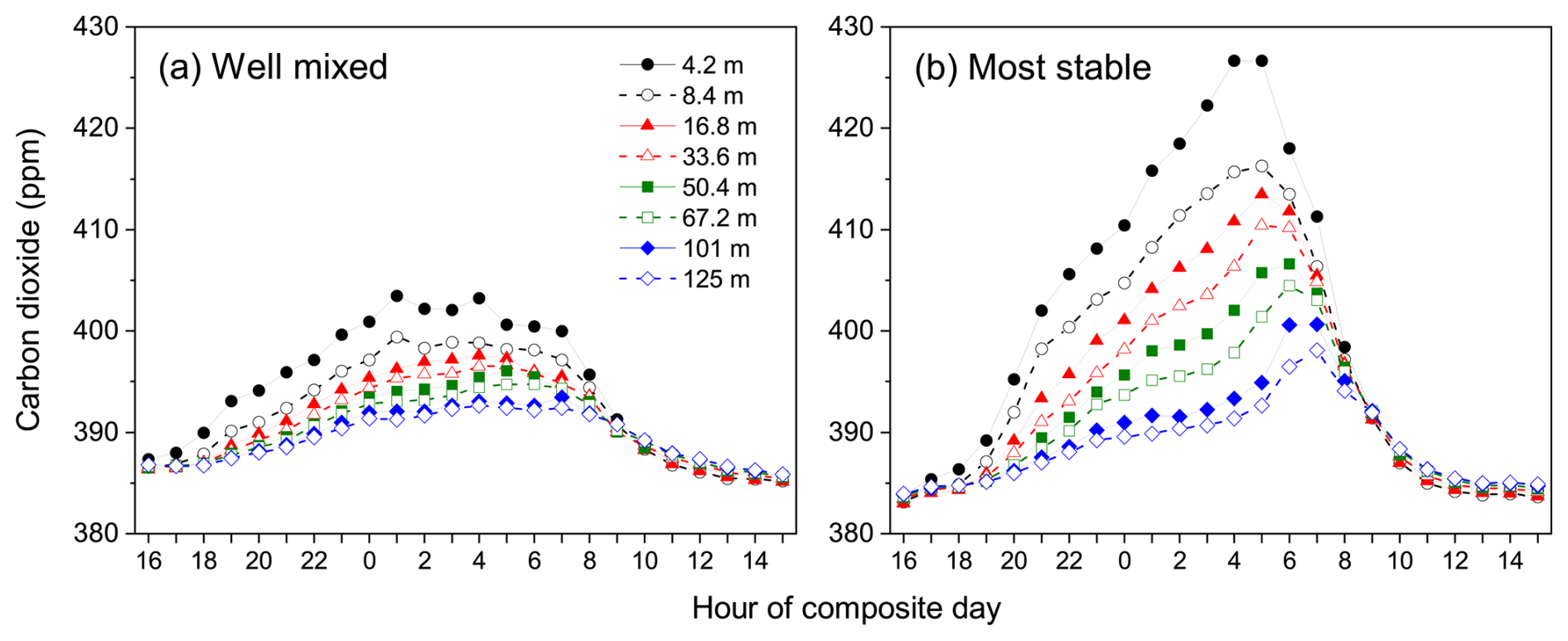
Figure 15 Growing season diel composite (hourly mean) CO₂ concentrations within and above a coniferous forest in Finland under well mixed and stable nocturnal conditions.

In the case of dense or complex urban canopies the combination of increased surface roughness and anthropogenic heat flux results in the nocturnal inversion that forms the upper bound of the urban boundary layer (UBL) being higher than the SNBL of the surrounding regions (providing a larger volume to dilute surface emissions). Built environments also contain more sealed surfaces (concrete, bitumen, etc.), which can restrict the rates of radon emission. Consequently, the amplitude of urban diurnal radon cycles is typically much smaller than comparable ones in surrounding areas (e.g. Fig. 3a; Chambers et al., 2019a).

Unlike forest canopies, trace gas sources associated with urban canopies are typically either surface based, or near rooftop height. Consequently, whether the RTM is applied within the urban canopy layer (UCL) or the UBL (e.g. Fig. 8.6; Oke, 1987) will be application specific. For measurements conducted in the UCL, near the centre of an urban region, the contributing fetch region will be reduced, and the percentage of sealed surfaces within this fetch greater, which may require a modification of the employed radon source function. The contributing fetch region for measurements made within the UBL will be larger (typically beyond the limits of the urban region for all but the most stable conditions) and contain a greater fraction of open soil surfaces, so modification of the regional radon source function may not be necessary.

3.5 The RTM contributing fetch

The contributing fetch in the traditional definition of the RTM (Sect. 2.1) is not explicitly considered. The result is understood to be a weighted average flux from an unspecified region of influence. However, the primary value of the RTM is as an independent TD method for estimating GHG emissions that can be used to verify BU estimates. For a quantitative comparison to be possible between these techniques, representative dimensions of the RTM's contributing fetch need to be determined so that the underlying contributing emissions can be identified and aggregated (Levin et al., 2021).

For this purpose, contemporary studies (e.g. Grossi et al., 2018; Levin et al., 2021; Yver-Kwok et al., 2024) have relied primarily on particle dispersion models such as STILT or FLEXPART (Lin et al., 2003; Brioude et al., 2013). However, while model biases are generally minimised under near-neutral through to weakly-stable conditions, when turbulence is vertically continuous and connected to the surface, the largest uncertainties arise under more strongly stable conditions - the very conditions under which most of the underlying assumptions and selection criteria for application of the local RTM are best met. The relatively low-resolution meteorological forcing (from operational re-analyses) employed by these dispersion models are not capable of capturing/representing the small scale spatial and vertical variability that occurs under stable atmospheric conditions.

Consequently, under strongly stratified atmospheric conditions models typically overestimate near-surface wind speeds (Kikaj et al., 2025b; Chambers et al., 2019b), potentially leading to significant overestimation of contributing fetch dimensions. Furthermore, the operational re-analyses don't resolve topography well (or changing surface roughness, which may impact simulated wind directions, e.g. Fig. 6a), and under stable nocturnal conditions topographically induced (katabatic) flows can dictate contributing fetch. Consequently, where observations are made lower in the SNBL (e.g. below 30–50 $\mathrm{m}\mathrm{a}.\mathrm{g}.\mathrm{l}.$), an argument could be made to rely more heavily on observed, stability classified wind speed information. Informed by category-mean stability classified wind speeds at the observation height, likely radii of influence could be overlain on simulated fetch regions as a more representative guide to the region of influence, providing a similar result to Fig. 1a of Levin et al. (2021). For strongly stable conditions over flat terrain wind directions can be highly variable, so a radius of influence based on mean wind speeds over the AW may be the best way to identify the lower bound of potential contributing sources.

According to Sesana et al. (2003), trace species with near surface sources only accumulate locally within the SNBL when near-surface wind speeds are below 1.5 m s⁻¹. To demonstrate this behaviour, 4 years of stability classified 2 $\mathrm{m}\mathrm{a}.\mathrm{g}.\mathrm{l}.$ wind speed and radon concentrations (excluding winter months) from at a flat, rural site in central Poland are summarised in Fig. 16 (see Chambers et al., 2016 for further information). On strongly stable nights near-surface wind speeds reduced to around 0.3 m s⁻¹, and radon accumulation up to 12 Bq m⁻³ above the previous afternoon minimum was observed. By contrast, under well-mixed conditions when mean nocturnal near-surface wind speeds were 1.1–1.2 m s⁻¹, a nocturnal radon accumulation of only 1.2 Bq m⁻³ was observed.

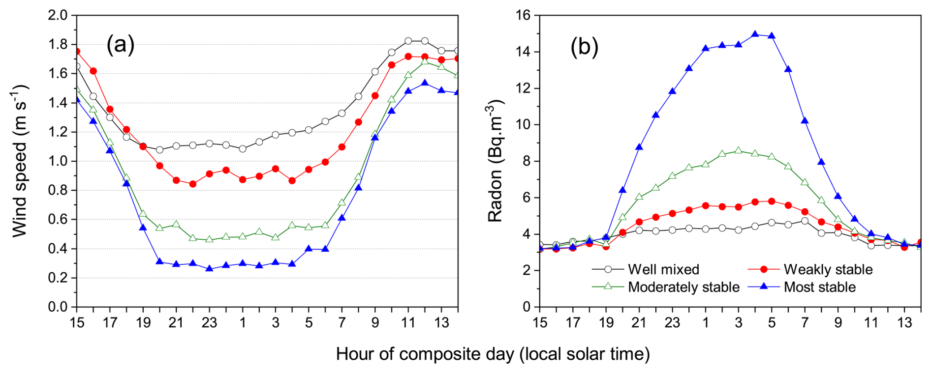
Figure 16 Diel composite 2 m (a) wind speed, and (b) radon concentration, as a function of contrasting nocturnal stability conditions for non-winter months at a rural site in central Poland over the 4 year period 2008–2011.

Typically, strongly stable nights occur under the influence of anti-cyclonic conditions (characterised by clear skies and regional subsidence). Synoptic winds, and their near-surface vertical gradients, are typically small within the shallow inversion layer. As described by Williams et al. (2013), if wind speeds just above, or within the inversion significantly increase, turbulence will develop and the SNBL will temporarily recouple with the overlying residual layer. As a result, accumulation near the surface would be interrupted or, in extreme cases, completely reset.

In comparable studies over flat, inland regions, 10 m wind speeds under strongly stable conditions were only around 0.5 m s⁻¹ (Chambers et al., 2015), and at 30 m around 1.5 m s⁻¹ (Chambers et al., 2016b). At Cabauw (Fig. 6b) wind speeds at 10 m and 20 $\mathrm{m}\mathrm{a}.\mathrm{g}.\mathrm{l}.$ for strongly stable conditions were around 1.5 and 2 m s⁻¹, respectively. Consequently, in the absence of substantial katabatic drainage flows, fetch regions for observations conducted under strongly stable conditions over an 8 h accumulation window are unlikely to have an extent of more than 10–40 km. In support of this hypothesis, Fig. 5d shows that under the most stable conditions the 20 m observations at Cabauw see very little influence from the urban regions ∼ 30 km to the south. This is in stark contrast to studies such as Grossi et al. (2018) that indicate contributing fetch regions of several hundred kilometres for accumulation measurements 20 m a.g.l. under reportedly stable conditions.

Historically, RTM applications have not imposed wind speed criteria. Furthermore, contemporary RTM applications are increasingly removing the requirement of atmospheric stability altogether, relying more on the quality of the linear correlation between radon and the tracer. The disadvantage of this approach is that the results obtained become an aggregate of contributions from all scales of fetch (which can range from tens to many hundreds of kilometres; e.g. Grossi et al., 2018; Levin et al., 2021). This causes significant, potentially retrievable information, to be lost. Alternatively, grouping nights according to a radon-based stability criteria (see Sect. 2.3) could both improve the quality of RTM estimates, and provide more detailed information about contributing fetch regions (over which emissions characteristics can change substantially).

3.6 Spatial and temporal variability of the radon flux

Equation (5) demonstrates that uncertainty in the footprint-weighted radon flux is directly proportional to uncertainty in the RTM target species flux estimate. Long-term spatial variability in radon flux is predominantly determined by the soil radium-226 content and physical characteristics (Nazaroff, 1992). Except for regions subjected to substantial anthropogenic disturbance (e.g. covering, reworking or backfilling of soils), this information is generally well characterised by the growing number of radon flux maps (Schery and Wasiolek, 1998; Szegvary et al., 2009; Griffiths et al., 2010; López-Coto et al., 2013; Karstens et al., 2015; Karstens and Levin, 2024). Temporal variability in radon flux, however, is primarily controlled by the soil moisture content and water table depth (Karstens et al., 2015; Karstens and Levin, 2024), which changes on seasonal, synoptic and diurnal timescales. Secondary influences associated with wind speed and pressure changes can also be significant on a range of timescales (Porstendörfer, 1994; Redeker et al., 2015).

While process-based radon flux maps in conjunction with soil moisture models are continually improving their representation of monthly-to-seasonal changes in radon flux associated soil moisture variability on corresponding timescales (e.g. Karstens et al., 2015; Karstens and Levin, 2024), failure to represent changing soil moisture conditions on sub-synoptic timescales (associated with individual rainfall events), or daily timescales (associated with diurnal evaporation), particularly in the summer months, can add a further factor of 2 uncertainty to existing uncertainties in spatial and temporal variability ( $\pm \mathrm{25}\mathit{\%}-\mathrm{30}\mathit{\%}$ seasonally), and contributing footprint flux definition (Levin et al., 2021).

Observed contrasts between different contemporary soil moisture reanalyses demonstrate the uncertainty in the absolute soil moisture (or free pore space), which can have a significant impact on quantitative tracer flux estimation. One way to improve understanding of this uncertainty and eventually improve the radon flux maps and parameterisations of key processes could be through the combined use of inverse modelling and long-term, high-quality atmospheric radon activity observations (Maier et al., 2025). Until the effects of soil moisture variability and uncertainty are better understood, this potentially represents a significant limitation to application of the RTM.

For the RTM applied as intended (i.e. under strong nocturnal stability conditions), some inherent safeguards exist against rapid short-term changes in radon flux associated with rainfall, wind speed, and pressure. Strong nocturnal stability is usually associated with anti-cyclonic synoptic conditions, characterised by stable high pressure, regional subsidence, clear skies, warm dry days, cold calm nights. Furthermore, the comparatively restricted fetch associated with strongly stable conditions increases the likelihood that meteorological conditions (particularly rainfall and wind) will be similar over this contributing area, and radon fluxes more homogeneous (Schmidt et al., 2001). Conversely, if the scope of conditions to apply the RTM is broadened to include well-mixed through moderate stability, this increases the likelihood of rainfall, gusty winds, and rapid pressure changes – which can modify the radon flux along the air mass trajectory. The final flux estimate would reflect a mixture of these influences over a larger contributing fetch.

The effect of nocturnal stability on wind speed was shown in Fig. 16a. To demonstrate stability influence on rainfall (and thereby short-term soil moisture variability), Fig. 17 contrasts diel composite rainfall in Ljubljana, Slovenia, over 2 years under a range of nocturnal stability conditions. On average, PTI conditions prevailed 25 % of the time in winter and autumn, and these events were excluded. “Non-stationary” days included a sharp synoptic transition (e.g. meteorological “front”) or pronounced air mass fetch change during the night.

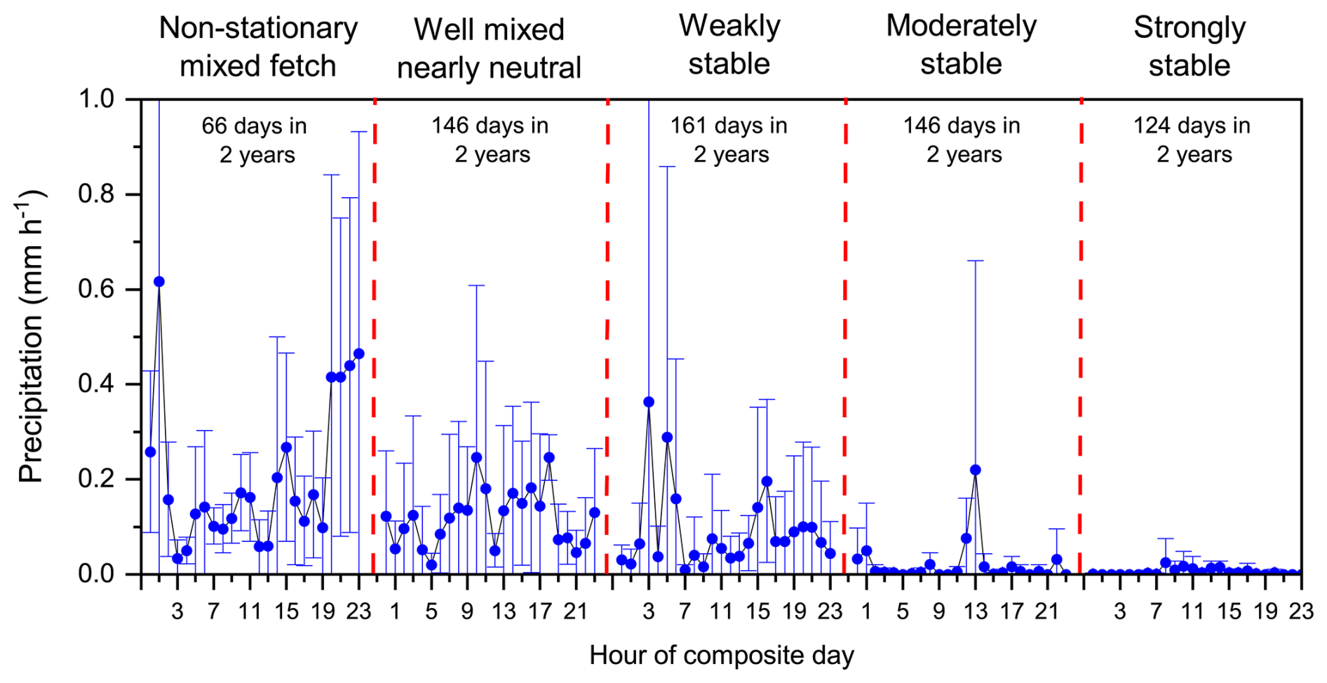
Figure 17 Diel composite hourly mean rainfall in Ljubljana (Slovenia) over 2017 and 2018 grouped by radon-derived stability categories.

Table 1 of Kikaj et al. (2020) summarises typical meteorological conditions for each stability class. Clearly, rainfall under strongly stable conditions was uncommon. Consequently, for a given month of the year, while long term (seasonal) changes in soil moisture would still be represented, selecting the most stable nights for RTM analysis would yield the least short-term variability in radon flux; i.e. radon fluxes that would be most closely represented by process-based flux maps. While rainfall distribution, and its impact on soil moisture variability, is not similarly distributed between seasons, the relationship between stability conditions and reduced rainfall is (Fig. 17). So, while there is no substitute for long-term, high temporal resolution radon flux observations representative of all weather conditions and soil types of the contributing fetch area (Levin et al., 2021), appropriate selection of conditions for which to apply the RTM can alleviate the problem. The “fair-weather bias” of strongly stable conditions should be kept in mind though, since it is not necessarily independent of GHG fluxes, given that cold, clear nights could give rise to higher anthropogenic CO₂ emissions and lower CH₄ emissions. Furthermore, as mentioned in Sect. 3.4, different nocturnal stability regimes often experience strongly contrasting contributing fetch directions and extent, due to changes in prevailing synoptic meteorology (Crawford et al., 2023; Kikaj et al., 2023).

3.7 Temporal representation of RTM emission estimates

At most the RTM yields one flux estimate per night, and traditional data selection criteria often reject 85 %–90 % of observations, leaving 3–4 suitable nights per month. If radon-based stability classification is adopted, this typically yields ∼ 3 nights per month per stability category (see Fig. 2). Consequently, the minimum temporal resolution for RTM-based flux estimates is monthly, although 2 monthly or seasonal estimates would be more statistically robust. Consequently, long-term, high-quality observations are critical. The soil-moisture driven uncertainties in radon flux (Sect. 3.6) make the RTM a tool that is better suited to characterising relative long-term (year-to-year) changes in emissions, rather than short-term absolute emission strengths. For this reason, the technique is not well suited to short, campaign-style observations (unless the sites are subsequently being returned to under comparable conditions year after year).

As an example of the pros and cons of changing temporal resolution, the 3 month average (June through August 2022, based on 9 separate events) CH₄ flux from 100 m on the Saclay tower under the most stable conditions was $(\mathrm{1.23}\pm \mathrm{0.22})\mathrm{mg}\left({\mathrm{CH}}_{\mathrm{4}}\right){\mathrm{m}}^{-\mathrm{2}}{\mathrm{h}}^{-\mathrm{1}}$. Performing the same analysis by month (each based on 3 samples) yields: June: $(\mathrm{1.40}\pm \mathrm{0.62})\mathrm{mg}\left({\mathrm{CH}}_{\mathrm{4}}\right){\mathrm{m}}^{-\mathrm{2}}{\mathrm{h}}^{-\mathrm{1}}$; July: $(\mathrm{1.18}\pm \mathrm{0.31})\mathrm{mg}\left({\mathrm{CH}}_{\mathrm{4}}\right){\mathrm{m}}^{-\mathrm{2}}{\mathrm{h}}^{-\mathrm{1}}$; and August: $(\mathrm{1.10}\pm \mathrm{0.26})\mathrm{mg}\left({\mathrm{CH}}_{\mathrm{4}}\right){\mathrm{m}}^{-\mathrm{2}}{\mathrm{h}}^{-\mathrm{1}}$. Clearly, fetch characteristics for the events contributing to each month's measurement could be analysed separately, along with the prevailing climatology, to determine how well the changing monthly values could be explained by changing source distributions in the respective contributing fetches, but it is beyond the scope of this study.

3.8 Requirements of radon monitors

An important consideration for the RTM is the expected nightly accumulation rates at a particular site or elevation (Sect. 3.2). The further measurements are from the surface, or the weaker the stability, the smaller the hourly accumulation rate and the greater demands on instrument sensitivity.

To maximise opportunities for RTM emission estimates, both purpose-built sites and existing long-term monitoring network stations (e.g. GAW, ICOS, UK DECC) should be utilised. However, depending on their location and fetch characteristics, not all existing tall-tower sites are equally suitable (see Sect. 3.4), and their measurements are often far from the surface.

Here we contrast required instrument performance characteristics for RTM observations at 15 and 100 m on the Saclay ICOS tower. In summer, CH₄ accumulation at 100 m between 22:00 and 05:00 LT was 20–30 ppb for moderate to strong stability (Fig. 11b), corresponding to accumulation rates of 2.5–3.8 ppb h⁻¹. Based on the typical repeatability of ICOS CH₄ observations (∼ 0.1 ppb; Yver-Kwok et al., 2015), this accumulation rate could be characterised reliably. The corresponding radon accumulation was 1.3–2 Bq m⁻³ (or 0.16–0.25 $\mathrm{Bq}{\mathrm{m}}^{-\mathrm{3}}{\mathrm{h}}^{-\mathrm{1}}$). Radon monitors capable of reliably measuring such accumulation rates are not common.

Calibration traceability for commercial radon monitors, for indoor public health research, was achieved to 100 Bq m⁻³ (MetroRADON; http://metroradon.eu, last access: 7 October 2025). Since these monitors have a > 40 % hourly measurement uncertainty at concentrations of 5 Bq m⁻³, separate “research grade” monitors have been developed for environmental measurements: two-filter monitors (Whittlestone and Zahorowski, 1998); electrostatic deposition monitors (Pereira and da Silva, 1989; Vargas et al., 2004; Wada et al., 2010); and single-filter α and β detecting monitors (Polian et al., 1986; Levin et al., 2002; Paatero et al., 1994). The often labelled “direct” radon monitors, since they sample ambient radon not radon progeny (e.g. based on the two-filter or electrostatic deposition principles) measure only newly-formed radon progeny in their measurement volumes under carefully controlled conditions (regarding ambient aerosol loading), making their observations independent of measurement height and weather conditions, whereas “indirect” monitors (single-filter) infer ambient radon concentrations from ambient radon-progeny measurements (Schmithüsen et al., 2017).

Traceability for direct research grade radon monitors was recently achieved to ∼ 1 Bq m⁻³ (traceRadon, http://traceradon-empir.eu/, last access: 7 October 2025; Röttger et al., 2021; Röttger et al., 2025). Furthermore, to enable these calibrations to be transferred to other monitors in the field, traceRadon developed two calibration transfer standard (CTS) devices: the ANSTO 200L monitor (Chambers et al., 2022), and the UPC ARMON v2 (Curcoll et al., 2024).

The most common research grade monitors at GAW and ICOS sites are currently the 1500L two-filter ANSTO monitor (Whittlestone and Zahorowski, 1998), and the Heidelberg Radon Monitor (HRM; Levin et al., 2002). Since the 1500L monitors have been too large to characterise in a controlled climate chamber, historically, ANSTO has defined the detection limit of their monitors to be the radon concentration at which the counting error reaches 30 %; rather than adopting the ISO 11929 definition. According to this definition, the detection limit of 1500L two-filter monitors is typically 0.025 Bq m⁻³ (Chambers et al., 2014), and their response time 45 min (correctable in post-processing; Griffiths et al., 2016) (see also rdfix software at https://github.com/anstoradonlab/rdfix; last access: 17 July 2026). Until recently, the large size and high flow rates of 1500L monitors have necessitated in situ calibration on top of the flow of sample air (with associated uncertainties of 2 %–8 %), but with the advent of CTS devices and pulse calibration techniques (Röttger et al., 2025) this uncertainty can now be largely eliminated. By comparison, the detection limit of the HRM (also based on a 30 % counting uncertainty) is 0.06–0.07 Bq m⁻³ (Chambers et al., 2018; Grossi et al., 2020). While the absolute accuracy of this indirect monitor is affected by radon-progeny disequilibrium below ∼ 80 $\mathrm{m}\mathrm{a}.\mathrm{g}.\mathrm{l}.$ (Jacobi and Andre, 1963), tube loss effects (Levin et al., 2017), aerosol scavenging events (e.g. fog or rain), atmospheric stability, and fetch effects, with appropriate data selection it is well suited to RTM studies (Levin et al., 2021; Gachkivskyi et al., 2025).

Based on their detection limits, both the 1500L two-filter detector and the HRM are capable of reliably characterising rates of radon accumulation at 100 m on the Saclay tower under conditions of moderate to strong stability (0.16–0.25 $\mathrm{Bq}{\mathrm{m}}^{-\mathrm{3}}{\mathrm{h}}^{-\mathrm{1}}$). However, the most consistent coverage for all meteorological conditions is provided by the ANSTO 1500L monitor.

Since space for instrument installation can be limited at existing tall-tower network sites, we also wanted to evaluate the potential suitability of the two direct portable CTS devices for tall-tower RTM studies, as well as for broader atmospheric research applications with stringent uncertainty demands. For this purpose, we briefly report on a previously published portion of an intercomparison between a 1500L two-filter detector and the two traceRadon CTS devices (the ANSTO 200L and the ARMON v2 monitors) (Fuente et al., 2022; http://traceradon-empir.eu/wp-content/uploads/2022/10/traceRadon_Newsletter_2022-09.pdf; last access: 2 March 2026). A full analysis of the complete 4 month intercomparison dataset, including a full uncertainty budget for the monitors, is out of scope for this paper but is currently in preparation as part of a separate study.

Figure 18a compares hourly aggregated observations between the 3 monitors for 7 of the first 38 d of the traceRadon Project's second field intercomparison project (ICP). Only a 7 d period in July 2022 was selected for Fig. 18a so that the individual hourly values are still discernible for direct comparison. Traceable calibrations for both the ANSTO 200L and ARMON v2 developed in a controlled climate chamber (Röttger et al., 2025) have been used for this dataset, and this calibration of the ANSTO 200L detector was transferred to the ANSTO 1500L (without interrupting its operation). Figure 18b and c compare regressions between the 1500L monitor and the portable CTS devices. The regression coefficients for the 1500L vs. 200L comparison demonstrate the successful calibration transfer.

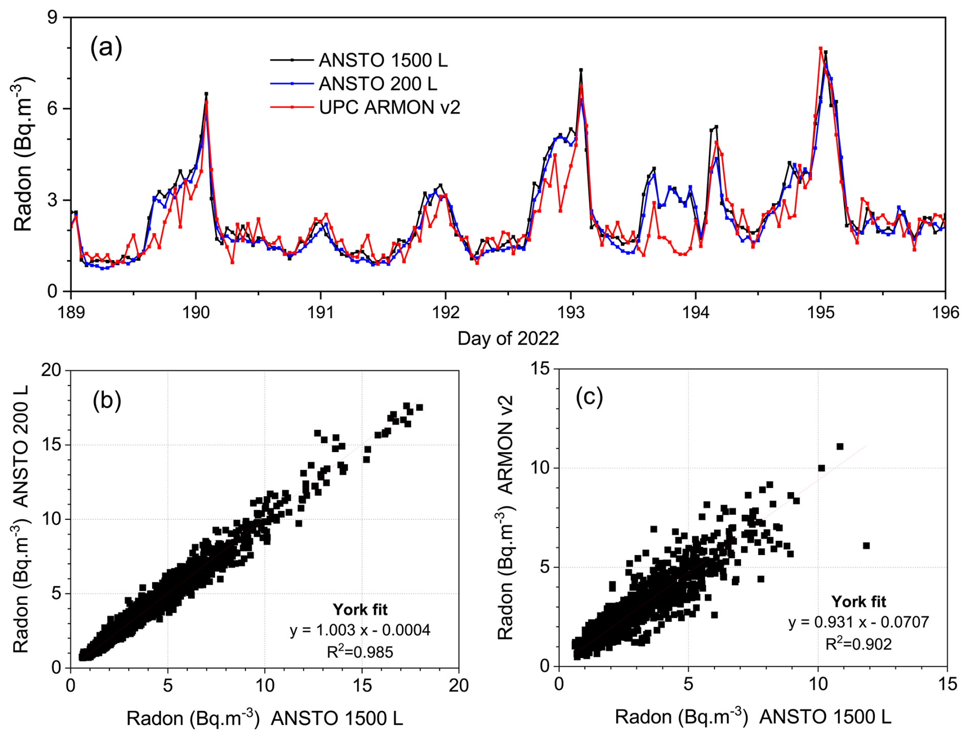
Figure 18 (a) 7 d comparison of hourly radon observations from 100 m on the Saclay tower between ANSTO 1500L and ANSTO 200L two-filter detectors and the UPC ARMON v2. (b) Linear regressions between the ANSTO 200L and ANSTO 1500L monitor (over the complete 4 month ICP), and (c) linear regressions between the ARMON v2 and the ANSTO 1500L for only 38 d of the ICP (ICOS, 2018, 2025; Ramonet et al., 2025). Full ICP dataset for the ARMON v2 will be presented in a subsequent manuscript currently in review.

The ANSTO 1500L and ANSTO 200L monitors shared one sampling line, while the ARMON v2 used a different line (shared with the HRM), all sampling from the same height on the tower. As expected, both two-filter detectors agreed well after the calibration transfer (Fig. 18b), with a slight scatter about the linear trend (R²=0.985) due to (i) the higher counting uncertainty of the 200L monitor, and (ii) slightly increased uncertainty of the response time correction based on the increased signal to noise ratio for the 200L monitor. A good agreement was also seen between the 1500L detector and the ARMON v2 (slope 0.932), but with a larger scatter about the linear trend (R²=0.901), attributable in part to the smaller ARMON v2 counting statistics.

Two-filter detectors have a 45 min response time, but both signals in Fig. 18 had been corrected for response time effects via deconvolution (Griffiths et al., 2016; Griffiths, 2024), which has slightly increased their individual measurement uncertainties (contributing to the lower R²-value in Fig. 18b). No response time correction is required for the ARMON v2. To determine whether any of the scatter observed in Fig. 18c could be attributed to differences in instrument response times (after correction of the two-filter detector signals), we sought an objective way of comparing the relative performance of these instruments. For measurements in the ABL spectral analysis (via Fast Fourier Transform, e.g. Press et al., 1992) can be used to assess the fidelity with which atmospheric monitors can reflect real physical changes associated with turbulent motions. For meteorological quantities and trace gases, observed signal variance in the ABL is contributed to by a range of scales (or time periods) of turbulence (Stull, 1988). Turbulence theory dictates that the signal power contributing to observed variance should decrease linearly (on a log–log plot) with decreasing scales of motion (or time periods). Deviation from this linearity (e.g. an upward flattening of the power spectrum curve), is indicative of instrumental noise (or uncertainty). We therefore performed a Fourier decomposition of the hourly Saclay radon record for each instrument, together with selected meteorological quantities, as a comparison (Fig. 19).

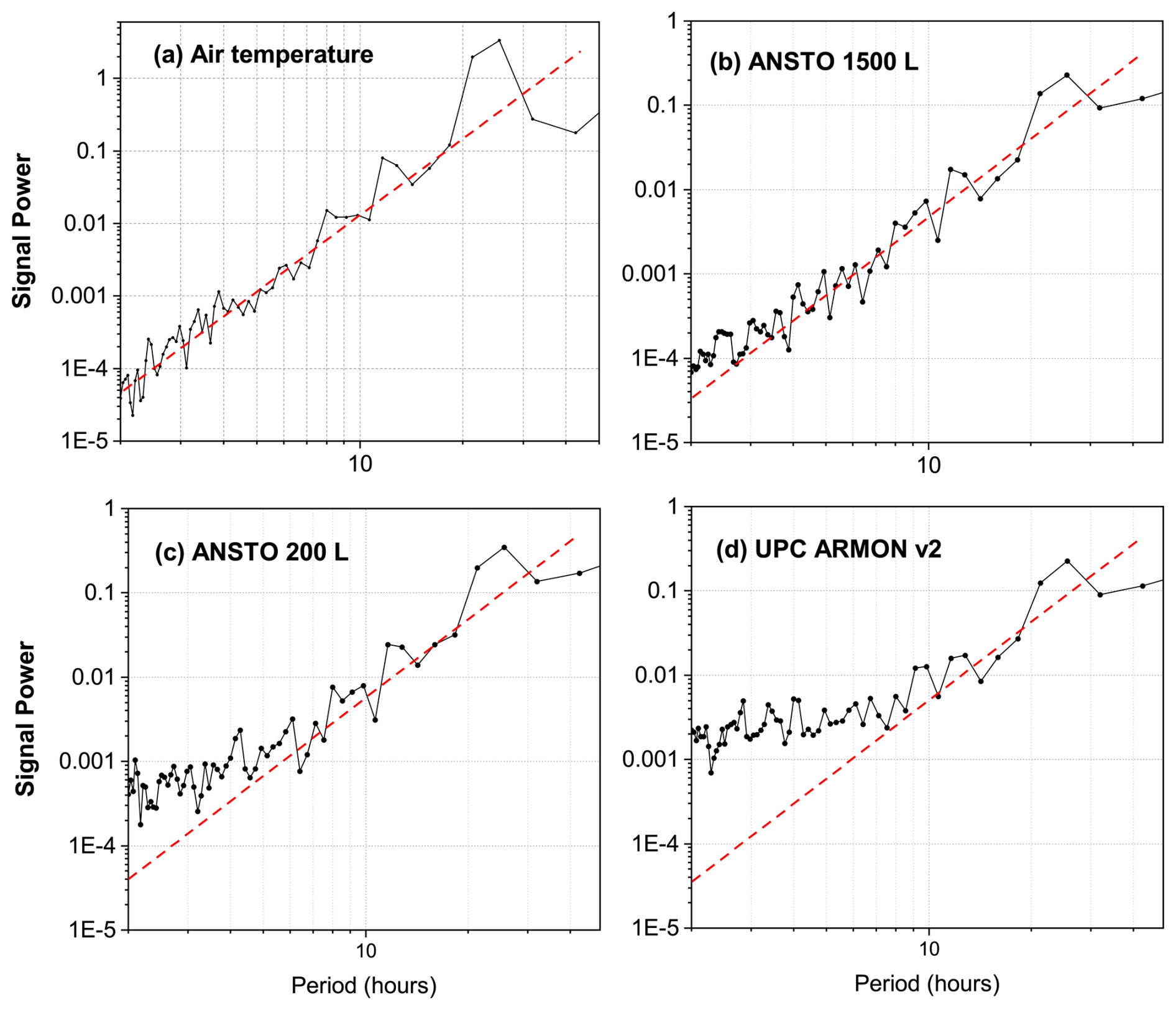
Figure 19 Power spectral density plots (variance signal power as a function of period of motion – from 2 h to > 1 week) based on hourly observations at 100 m from the Saclay ICOS tower. (a) the ICOS 100 m Saclay temperature record, (b) an ANSTO 1500L monitor, (c) an ANSTO 200L monitor, and (d) the UPC ARMON v2. Hand-drawn red dashed linear trends have been included to guide the eye.

Temperature measurements at 100 m on the Saclay tower were checked for consistency prior to the Fourier decomposition, and no evidence of significant inaccuracy or non-conformity was identified. Consistent with theoretical expectations, contribution to observed temperature variance (signal power) for all sub-diel (< 24 h) periods decreased approximately linearly with decreasing period (i.e. towards smaller turbulence scales; Fig. 19a). This behaviour is consistent with temperature variability dominated by turbulent mixing in the atmospheric boundary layer. Results for humidity have not been shown here but are available in the companion dataset (Chambers, 2025).

The ANSTO 1500L monitor output exhibited an approximately linear reduction of signal power with period of turbulent motion (Fig. 19b), similar to that observed for temperature at the same height. This behaviour is consistent with the reported radon variability being primarily driven by the same physical atmospheric processes that control temperature variance. Relative to this behaviour, the ANSTO 200L and ARMON v2 spectra showed increasing deviation at shorter periods, with the largest departure observed for the ARMON v2. These differences are consistent with a progressive reduction in fidelity for resolving short-timescale, turbulence-driven radon variability from the ANSTO 1500L to the ANSTO 200L and then to the ARMON v2. The departure of the ARMON v2 spectrum from the linear trend at periods of 7–8 h in Fig. 19d is relatively consistent with several 6–10 h periods of large bias evident between the ARMON v2 and ANSTO 1500L monitor in Fig. 18 a. In this context, the mean absolute differences between the ANSTO 1500L and ANSTO 200L signals ($\mathrm{0.25}\pm \mathrm{0.24}\mathrm{Bq}{\mathrm{m}}^{-\mathrm{3}}$; Fig. 18a and b), and between the ANSTO 1500L and ARMON v2 signals ($\mathrm{0.53}\pm \mathrm{0.55}\mathrm{Bq}{\mathrm{m}}^{-\mathrm{3}}$; Fig. 18a and c), are more consistent with increasing instrumental limitations at shorter periods than with residual differences in instrument response time.

The sensitivity to radon of direct monitors such as the two-filter and electrostatic deposition types is a strong function of measurement volume. Together, the detector sensitivities and instrumental backgrounds are used to determine a counting uncertainty for each instrument. The measurement volumes of the three detectors compared here are 1500L, 200L and 20L. The respective sensitivity to radon of these instruments is 0.35 ${\mathrm{s}}^{-\mathrm{1}}(\mathrm{Bq}{\mathrm{m}}^{-\mathrm{3}}{)}^{-\mathrm{1}}$ for the ANSTO 1500L monitor, 0.0426 ${\mathrm{s}}^{-\mathrm{1}}(\mathrm{Bq}{\mathrm{m}}^{-\mathrm{3}}{)}^{-\mathrm{1}}$ for the ANSTO 200L monitor, and 0.0059 ${\mathrm{s}}^{-\mathrm{1}}(\mathrm{Bq}{\mathrm{m}}^{-\mathrm{3}}{)}^{-\mathrm{1}}$ for the ARMON v2 (Chambers et al., 2022; Röttger et al., 2025). As a first order approximation, the dominant reason for the ANSTO 200L and ARMON v2 monitors to be less able than the ANSTO 1500L monitor to accurately represent radon variability driven by decreasing scales of atmospheric turbulence is more likely their respective measurement uncertainties than a difference in response times between the instruments.

Having empirically established the superior measurement performance regarding sensitivity and relative response of the larger volume ANSTO 1500L monitor over the smaller ANSTO 200L detector (Fig. 19b and c; see Kikaj et al., 2025a for a discussion of 1500L monitors in the broader context), we now summarise a comparison of the ANSTO 200L and ARMON v2 monitors performed in the controlled climate chamber of Physikalisch-Technische Bundesanstalt (PTB, Braunschweig, Germany) (Röttger et al., 2025) and discuss how the difference in their performance observed at PTB could impact the performance of these more compact monitors for RTM applications.

The ANSTO 200L and ARMON v2 CTS devices were setup in the climate chamber along with a reference AlphaGUARD PQ2000 PRO monitor. Over a 4 month period, through a combination of novel low activity Radium-226 sources (Mertes et al., 2022) and zero-radon air, radon concentrations were varied between ∼ 0 and 45 Bq m⁻³ (Fig. 20a). Over the course of these tests, the standard deviation of the ARMON v2 radon concentrations relative to the simulated value chamber concentration (based on source activity and chamber free volume of 21.2 m³) was more than double that of the response-time corrected ANSTO 200L monitor (Fig. 20b). Under the PTB chamber's controlled conditions, this indicates broader scatter for the ARMON v2 and lower scatter for the ANSTO 200L.

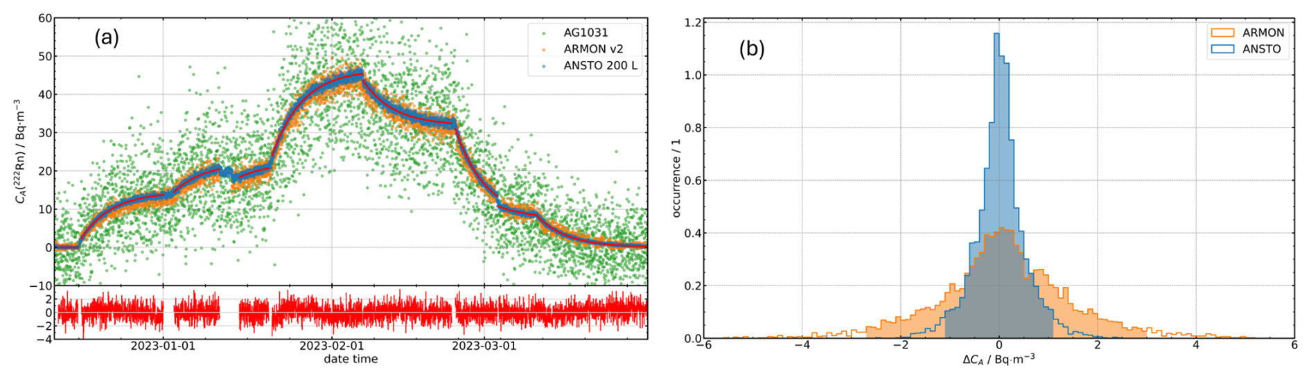
Figure 20 (a) 4 month comparison of the ANSTO 200L and ARMON v2 monitors in the PTB climate chamber, and (b) comparison of standard deviations about the simulated chamber radon concentration (adapted from Röttger et al., 2025).

We sought to determine whether this performance difference could affect instrument suitability for RTM studies, and if so, under what conditions. Radon accumulation rates at Saclay (100 $\mathrm{m}\mathrm{a}.\mathrm{g}.\mathrm{l}.$) between 22:00 and 05:00 LT under moderate to strong stability were 0.16–0.25 $\mathrm{Bq}{\mathrm{m}}^{-\mathrm{3}}{\mathrm{h}}^{-\mathrm{1}}$ at ambient concentrations of 3–4 Bq m⁻³ (Fig. 10). Based on the PTB instrument calibrations (Röttger et al., 2025), the uncertainty (k=1) of the ANSTO 200L and ARMON v2 monitors at 7.9 Bq m⁻³ (the lowest calibration point) was ±7.1 % and ±16.7 %, respectively. Conservatively, at 4 Bq m⁻³ this equates to an uncertainty of ±0.28 and ±0.67 Bq m⁻³, for the ANSTO 200L and ARMON v2, respectively. Under these assumptions, the uncertainty of the ANSTO 200L monitor is of similar magnitude to the expected 100 m Saclay accumulation rate under strongly stable conditions, whereas that of the ARMON v2 was around a factor of 3 higher than the expected accumulation rate under the same conditions.

To achieve an acceptable uncertainty for RTM applications, Levin et al. (2011), who originally conceived the RTM technique, recommended that the accumulation rate of change be a factor of 3 higher than the measurement uncertainty of the instrument being used to characterise it. While this benchmark is achievable for 100 m observations at Saclay under strongly stable conditions using an ANSTO 1500L monitor, it is not achievable by either the ANSTO 200L or ARMON v2 detectors. These conclusions should, however, be interpreted in the context of the concentration range, accumulation rates, and measurement height considered here.

However, if space limitations at a tall-tower site necessitate that one of the more compact CTS devices is used, then the strengths and weaknesses of each of the CTS devices should be carefully considered. While the ANSTO 200L monitor has a lower measurement uncertainty and does not require a dry air stream for operation, the ARMON v2 is more portable (shorter and lighter), and has alpha-spectroscopic abilities (which can distinguish between radon isotopes) that the ANSTO radon monitors lack. More generally, the suitability of compact radon monitors for RTM applications will depend on the magnitude of the radon accumulation rate relative to instrument uncertainty, which may vary with site-specific exhalation rates, boundary-layer dynamics, coastal versus inland setting, and sampling height. When applying less accurate radon monitors than the ANSTO  1500L to the RTM, the user should be mindful that increasing measurement uncertainty would necessitate the reduction of R² thresholds for the Rn-to-target gas regressions (see Sect. 3.3), and it could become increasingly difficult to separate outliers due to fetch heterogeneity from instrument uncertainty.

A complete comparative uncertainty analysis of RTM flux estimates at Saclay by each radon instrument is beyond the scope of this study. However, as an illustration of the behaviour described above, Fig. 21 compares two nights of observations at 100 m on the Saclay ICOS tower (24 and 27 July 2022), for which the R² value for radon-to-CH₄ regressions based on measurements by the ANSTO 1500L monitor were > 0.7. Plots on the left (Fig. 21a and d) are for the ANSTO 1500L monitor, plots in the middle (Fig. 21b and e) are for the ANSTO 200L monitor, and plots on the right (Fig. 21c and f) are for the ARMON v2. The higher uncertainty of the ARMON v2 measurements at the low radon concentrations experienced at 100 $\mathrm{m}\mathrm{a}.\mathrm{g}.\mathrm{l}.$, results in substantial changes in slope and R² values for the radon-to-CH₄ regressions.

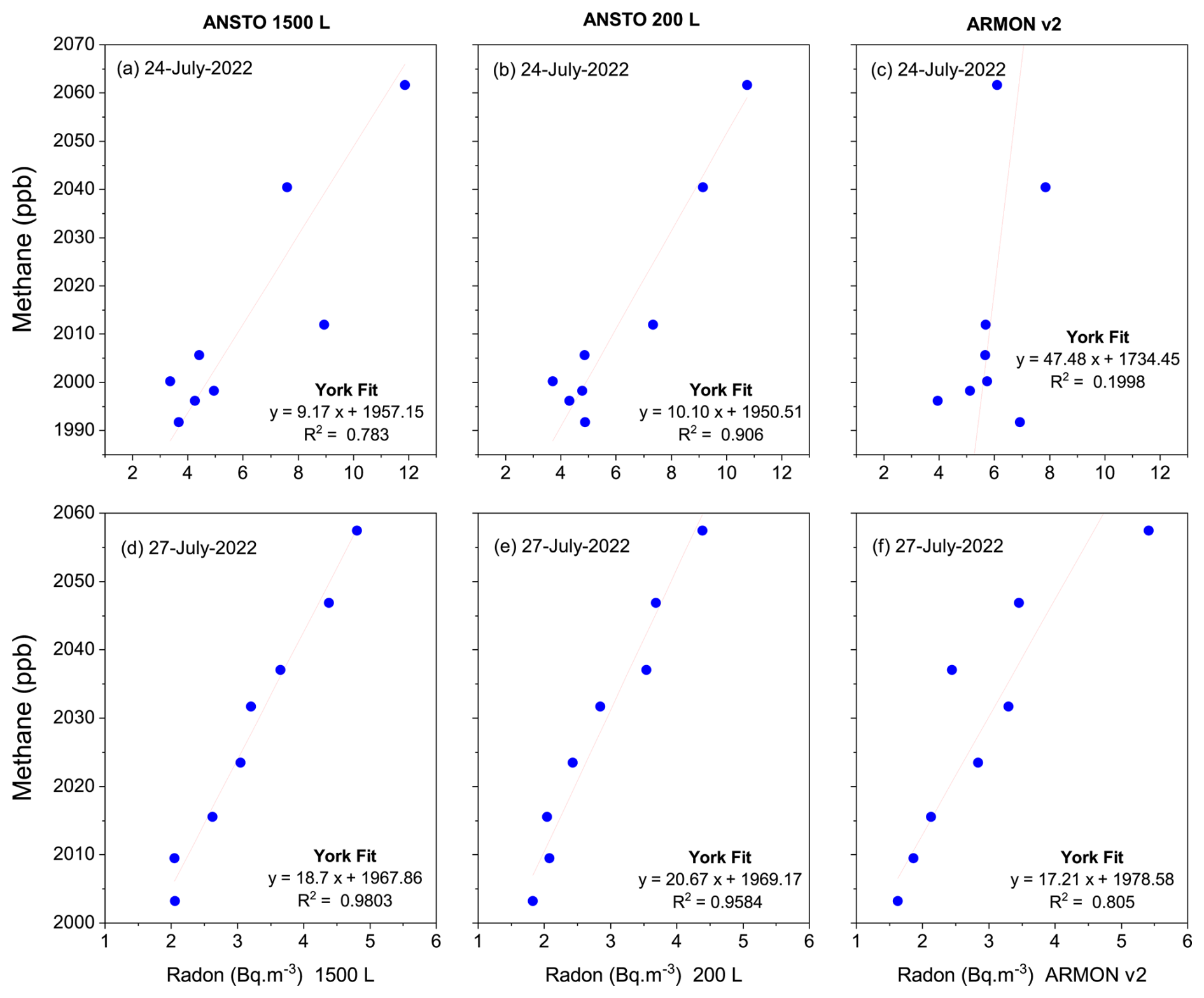
Figure 21 Radon-to-CH₄ regressions for two moderately stable nights between 22:00 and 05:00 LT at 100 m on the Saclay ICOS tower on the nights of 24 and 27 July 2022.

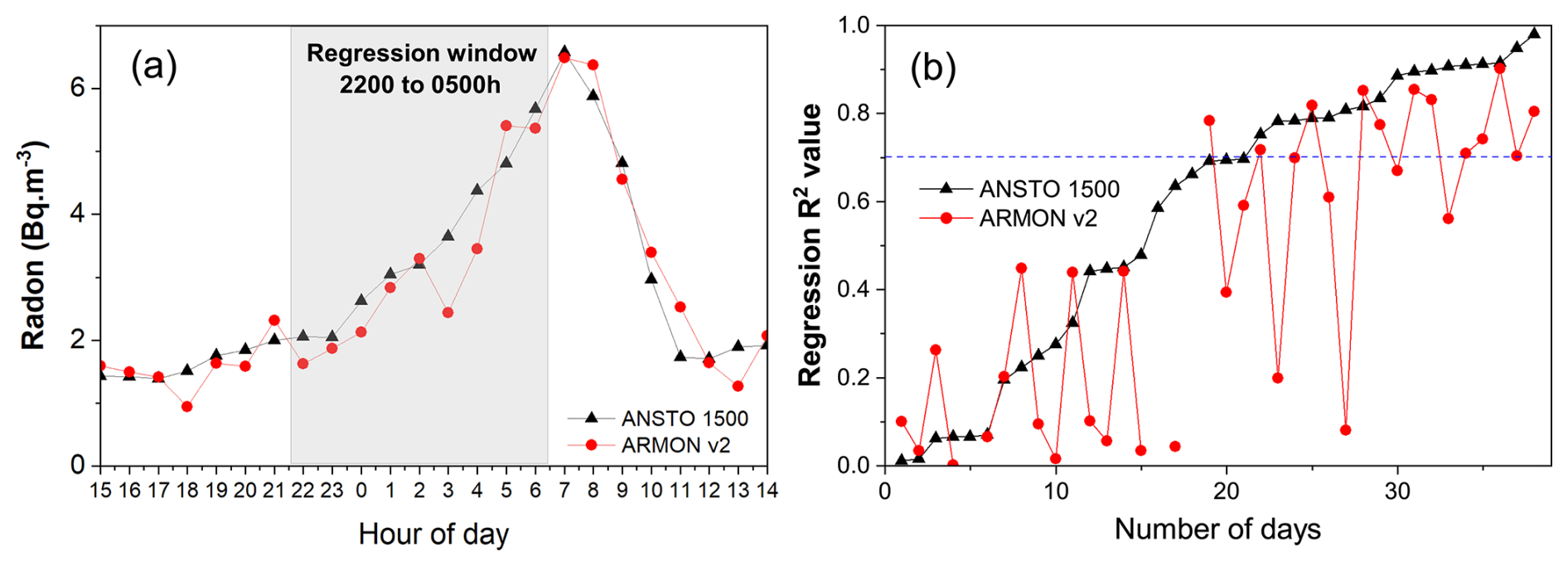
Figure 22 (a) Diurnal cycle of radon at 100 m on the Saclay ICOS tower on 27 July 2022 (see Fig. 21d), and (b) radon-to-CH₄ regression values (sorted in ascending order) for the first 38 d of the ICP based on observations from the ANSTO 1500L and ARMON v2 radon monitors.

To further illustrate the differences in slope and R² values between Fig. 21d and f, Fig. 22a shows the entire diurnal radon cycle at 100 m on the Saclay ICOS tower on 27 July 2022 as observed by the ANSTO 1500L and ARMON v2 monitors. The influence of the greater uncertainty of the ARMON v2 instrument is evident, and of a similar magnitude to that calculated from the PTB tests. Radon-to-CH₄ regressions were calculated each night for the first 38 d of the ICP over the 22:00–05:00 LT window for each monitor, and the corresponding R² values sorted according to the ANSTO 1500L monitor values (Fig. 22b). Results indicate a substantial reduction in number of nights with R² values greater than the nominal 0.7 threshold for observations made by the ARMON v2. To address this issue, lower R² thresholds may be required for radon monitors with higher uncertainty (e.g. 0.5 or 0.6). Since counting statistics are random in nature, averaging over many nights will reduce the error in regression slopes used to make the estimate fluxes. However, if data is to be analysed by month and stability category, there are often few suitable nights available for averaging.

Shifting focus from 100 $\mathrm{m}\mathrm{a}.\mathrm{g}.\mathrm{l}.$ observations to a lower inlet height (15 m) on the same tall tower, and using the Saclay observations as an example, radon accumulation was ∼ 3 times larger closer to the surface (3 and 6 Bq m⁻³ for moderate and strong stability; Fig. 10). Since the accumulation rate under stable conditions (0.75 $\mathrm{Bq}{\mathrm{m}}^{-\mathrm{3}}{\mathrm{h}}^{-\mathrm{1}}$) is higher than the corresponding measurement uncertainty at those concentrations for either the ANSTO 200L or ARMON v2, the more compact CTS devices would be better suited for RTM applications where measurements are made at lower inlet heights (e.g. 20 $\mathrm{m}\mathrm{a}.\mathrm{g}.\mathrm{l}.$, in Grossi et al., 2018). Another important consideration is the spatial variability of radon emissions across Europe (e.g. Karstens et al., 2015). In cases where the regional radon flux is considerably higher than in the footprint of the Saclay ICOS tower, accumulation rates under stable conditions further from the surface would be larger. Radon observations for purposes other than RTM studies will likely have application-specific requirements regarding temporal resolution and instrument uncertainty, necessitating a separate assessment of instrument suitability.

4 Conclusions

The Radon Tracer Method is an established, independent top-down method to estimate local- (e.g. urban scale) to regional-scale emissions of target species (e.g. greenhouse gases) that is relatively simple-to-apply. However, challenges associated with accurate characterisation of short-term spatial and temporal variability in radon flux estimates, largely associated with soil moisture variability (and related uncertainties), typically render the technique better suited to characterising long-term relative changes in emissions rather than short-term absolute emissions estimates. Despite this caveat, the RTM remains a valuable asset for sanity checking bottom-up emission inventories, assessing the efficacy of GHG mitigation strategies, and potentially demonstrating continual improvement in atmospheric transport model inversions of regional emissions as ATM uncertainties are reduced.

Key to success in these endeavours, however, is the ability to accurately characterise the contributing fetch (over which the radon fluxes are determined and the emission magnitudes estimated). Contemporary RTM studies are increasingly relying on particle dispersion models for this purpose despite inherent incompatibilities: the RTM is best suited to strongly stable conditions and model performance is worst under strongly stable conditions (with a tendency to overestimate or incorrectly assign contributing fetch). Furthermore, necessarily strict RTM selection criteria severely limit data availability, which typically leads to all available results being averaged over the representative time period, despite potentially being influenced by strongly contrasting fetch regions.

This article summarises, and discusses the significance of, the necessary considerations for planning and implementing emission estimates via the RTM: (i) definition of the nocturnal window; (ii) radon and target gas accumulation thresholds; (iii) radon-to-target gas regression linearity thresholds; (iv) measurement height; (v) the contributing fetch region; (vi) effects of spatial and temporal variability of the radon flux; (vii) temporal representation of RTM emission estimates; and (viii) application specific appropriate requirements for radon monitors. It also demonstrates numerous potential benefits of combining nocturnal atmospheric stability analysis with nocturnal accumulation types of RTM studies. In addition to clearer nocturnal window definition and reduced spatial/temporal variability of the radon flux over the contributing fetch, applying the RTM within designated nocturnal stability categories enables better constraint of simulated contributing fetch regions, and clearer attribution of calculated emission estimates to specific fetch regions, each of which stand to improve comparisons with bottom-up techniques.

As mentioned in the Introduction, the nocturnal accumulation implementation of the RTM is one of four implementations discussed in the literature. Others include: (1) a regional-to-continental scale boundary layer approach; (2) a regional scale plume/event-based approach; and (3) a local scale profile method. Not all considerations discussed in this manuscript apply equally to the other approaches. The profile method is also a nocturnal accumulation RTM formulation based on near-surface vertical gradients. As such it would also benefit from stability classification. Measurement heights are necessarily low (to limit the spatial extent of the contributing fetch), and the sensitivity of results to some of the remaining seven considerations would depend on the small-scale fetch heterogeneity. For a homogeneous region, considerations (i), (v) and (vi) above would be less significant. Although measurements are close to the surface (where radon concentrations are larger), since radon gradients need to be accurately characterised, low measurement uncertainty would also be important for this implementation.

Regarding the regional-scale implementations of the RTM, they both target observations in a well-mixed, fully developed boundary layer. As such, stability classification would not benefit these approaches. For the plume method it is usually necessary to minimise local influences (for which a wind speed threshold, based on measurement height, is usually applied, and measurements below this are excluded). The “accumulation threshold” requirement is usually replaced by a minimum concentration above the “baseline” value. A representative characterisation of the contributing fetch is still important (although at higher wind speeds, in a developed boundary layer, trajectory or plume dispersion model fetch estimates are likely to be more representative of “truth” than under stable nocturnal conditions). Similar challenges regarding the representation of spatial and temporal variability of the radon flux will remain. Air mass travel times are longer, more attention needs to be paid to radon decay in transit, and the measurement uncertainty for radon detection is usually less critical given the typically large differences between “baseline” and continental air masses.

ANSTO 1500L two-filter radon monitors and Heidelberg radon monitors are best suited to perform RTM studies from tall-tower sites. Closer to the surface (≤20 m) the ANSTO 200L two-filter and ARMON v2 monitors could also give reliable results (albeit with larger uncertainties). ANSTO 1500L monitors should be periodically calibrated with a calibration transfer standard device or pulse calibration method (Röttger et al., 2025) and the appropriate response time correction applied (Griffiths et al., 2016; see also the “rdfix” software at https://github.com/anstoradonlab/rdfix; last access: 17 July 2026). Since calibration transfer does not require the instrument to be taken offline, data retrieval rates would be improved. Maintaining traceable calibrations would improve the utility of the long-term radon observations beyond RTM applications, enabling higher-quality atmospheric baseline studies, and model inversions or model evaluation studies. Calibrations performed as part of the 19ENV01 traceRadon Project (Röttger et al., 2025) verified that both the ANSTO 200L and ARMON v2 monitors are equally well suited to act as CTS devices.

Appendix A

To recap, the underlying assumptions for applying the nocturnal accumulation RTM include:

• i.

  radon and target gas fluxes similarly distributed and relatively homogeneous over the contributing fetch;

• ii.

  any heterogeneity is small-scale and random, uncorrelated with atmospheric processes on small spatial/temporal scales;

• iii.

  the target gas has no atmospheric sinks over measurement timescales, or between emission and measurement;

• iv.

  both species are acted upon by the same transport and mixing processes from the source to the point of measurement (i.e. measured at the same, constant location and height above ground within the SNBL).

The site or application specific considerations discussed in this review are summarised below in Table A1.

Table A1 Summary of application-specific considerations for application of the nocturnal accumulation formulation of the Radon Tracer Method.

Appendix B

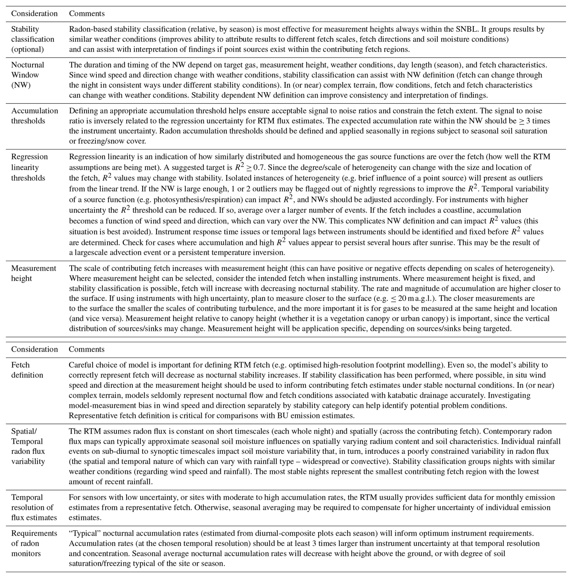
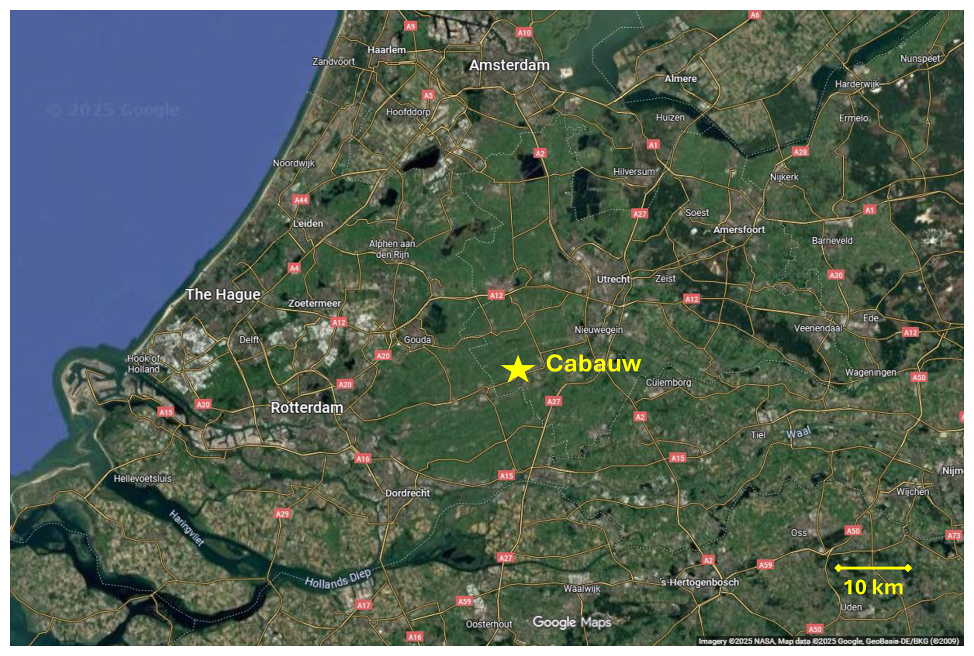
Figure B1 Location of the Cabauw ICOS tower relative to surrounding agricultural regions and the nearest urban regions. Google Maps (Imagery © 2025 NASA, Map data © 2025 Google, GeoBasis-DE/BKG; © 2009).