Improving simulations of Zeeman absorption spectrum for hyperspectral microwave sounding applications

Accurate simulation of microwave oxygen absorption is critical for upper atmospheric remote sensing, yet traditional models suffer from biases due to simplified Zeeman splitting calculations. This study presents the channel parameters of a hyperspectral microwave sounder for near space temperature profiling, built upon the updated microwave Line-by-Line (LBL) model with Larsson et al. (2019) Zeeman coefficients. The Hyperspectral Microwave Atmospheric Sounder (HMAS) is designed as a 60–63 GHz linearly polarized instrument comprising 150 channels, optimized to 39 composite channels for noise reduction. The HMAS channels are validated by comparing weighting functions and simulated brightness temperatures with Special Sensor Microwave Imager/Sounder (SSMIS) upper atmospheric sounding (UAS) channels. The global distribution of brightness temperature differences between HMAS composite channels and SSMIS channels on representative dates shows that the differences are generally within ±1.3 K, confirming the physical consistency of the HMAS channel design. Temperature profile retrieval experiments are conducted using an improved back propagation (BP) neural network with dual residual blocks and squeeze-and-excitation (SE) attention mechanism based on simulated brightness temperatures from both HMAS and SSMIS corresponding channels. The retrieval results show that the HMAS achieves a root mean square error (RMSE) of 7.652 ± 0.389 K, a mean absolute error (MAE) of 4.911 ± 0.282 K, and a coefficient of determination (R²) of 0.915 ± 0.010, while the SSMIS channels 19–24 yield a RMSE of 7.858 ± 0.314 K, a MAE of 5.107 ± 0.208 K, and an R² of 0.910 ± 0.010. The HMAS shows potential as a payload for future near space exploration missions.

1 Introduction

Near space typically refers to the region between 20 and 100 km (60–0.0004 hPa) above sea level, encompassing the stratosphere, mesosphere, and lower thermosphere (Yang et al., 2023). Observation of near space is crucial for weather forecasting and climate analysis (Eckermann et al., 2018; Liu et al., 2007; Zhao et al., 2021). The accuracy of upper atmosphere forecasts can be improved by assimilating near space observations in numerical weather prediction (NWP) systems (Eckermann et al., 2009; Hoppel et al., 2013, 2008; Maurer et al., 2015; Nezlin et al., 2009). However, observations of the middle to upper atmosphere are comparatively rare due to technological and scientific limitations (Dong et al., 2024). Satellite-based data used in NWP assimilation systems at altitudes above 1 hPa are typically from the Microwave Limb Sounder (MLS), the Sounding of the Atmosphere using Broadband Emission Radiometry (SABER), and the Special Sensor Microwave Imager/Sounder (SSMIS) on board the Defense Meteorology Satellite Program (DMSP) satellite (Hoppel et al., 2008). The temperature analysis fields from assimilated SSMIS upper atmospheric sounding (UAS) channels are comparable to those from SABER and MLS data (Hoppel et al., 2013). However, SSMIS has only six UAS channels with low vertical resolution and significant noise. Increasing the amount of high-quality upper atmospheric observation data is critical for weather forecasting and climate analysis.

Infrared hyperspectral instruments have now reached maturity, and their radiance data have been proven to improve NWP forecast accuracy (Aires et al., 2015; Eresmaa et al., 2017; McNally et al., 2006). Nevertheless, infrared observations are inherently limited by their shorter wavelengths, which are strongly attenuated by clouds and precipitation, making it difficult to obtain valid measurements under cloudy conditions. Microwave sensors, operating at much longer wavelengths, can penetrate clouds and precipitation, enabling all-weather observations and reaching higher altitudes. Thus, microwave sensors are essential for filling the observational gaps left by infrared instruments, particularly in cloudy conditions and the upper atmosphere. However, microwave sensors have significantly fewer detection channels compared to infrared instruments due to technological limitations (Boukabara and Garrett, 2011). With recent advancements in Fast Fourier Transform spectroscopy technology, microwave radiometers with high spectral resolution have become a more feasible component in remote sensing (Kummerow et al., 2022). This is highly beneficial because microwave hyperspectral sampling can achieve a high-density weighting function (WF), which facilitates the accurate retrieval of temperature and water vapor profiles and exerts a positive impact on weather forecasting (Aires et al., 2015; Zhang et al., 2025). In recent years, various studies have focused on specific hyperspectral microwave channels and their ability to provide valuable observations for retrieval or NWP systems (Bi et al., 2024; Blackwell et al., 2011; Boukabara and Garrett, 2011). However, most studies primarily reference the Advanced Microwave Sounding Unit (AMSU) or Advanced Technology Microwave Sounder (ATMS) temperature and water vapor detection channels (around 52.6–57.3 and 183.31 GHz), which mainly provide information on tropospheric clouds, precipitation, and surface parameters, with limited upper atmospheric information.

Microwave oxygen (O₂) absorption channel observations and simulations close to and above 40 km are affected by Earth's magnetic field. At lower altitudes, pressure broadening generally dominates over Zeeman splitting, reducing its influence on the polarized radiation. As pressure broadening weakens with increasing altitude, Zeeman splitting becomes increasingly important for upper atmospheric microwave sounding (Larsson et al., 2016). The 2 × 2 coherency matrix formed radiative transfer equation can describe the Zeeman splitting effect (Lenoir, 1967, 1968; Rosenkranz and Staelin, 1988). To fully investigate the influence of magnetic field parameters on brightness temperature (BT) simulation, Stogryn (1989) derived the magnetic field-related symmetry, systematically revealing the quantitative impact of Zeeman splitting on O₂ absorption line simulations (Stogryn, 1989). However, these earlier approaches rely on a simplified Hund's case (b) assumption, which has limitations for low rotational quantum numbers. Larsson et al. (2019) provided updated Zeeman splitting coefficients that account for fine-structure state mixing and additional Zeeman interactions (Larsson et al., 2019). A recent study conducted a detailed comparison of the simulation differences between the Hund's case (b) and the Larsson et al. (2019) implementation, including an analysis of the Stokes parameters for various oxygen absorption lines (Dong et al., 2026). In this study, the RS-LBL model (version 2024), updated with the Zeeman splitting coefficients of Larsson et al. (2019), is used to investigate oxygen absorption line characteristics. Section 2 describes the treatment of Zeeman splitting, oxygen absorption, and radiative transfer. Section 3 examines the sensitivity of oxygen absorption lines to the geomagnetic field and their altitude sensitivity. Section 4 presents the proposed microwave sounder channel configurations and evaluates the Hyperspectral Microwave Atmospheric Sounder (HMAS) through comparisons with SSMIS in terms of weighting functions, simulated brightness temperatures, and temperature profile retrievals using an improved back propagation (BP) neural network. Section 5 summarizes the main findings and limitations.

2 Methodology

2.1 Zeeman Splitting Effect

Under an external magnetic field, the Zeeman splitting effect causes the energy levels of oxygen molecules to split, with the emitted or absorbed radiation originating from the molecule's magnetic dipole (Zeeman, 1897). This phenomenon manifests as a single spectral line splitting into multiple sub-lines with distinct polarization characteristics, a process whose radiative influence becomes increasingly important as pressure broadening weakens with altitude.

The g-factor ($g_{J_{\mathrm{N}}}$) describes the first-order magnetic response of a specific fine-structure energy level J_N of oxygen molecules. It directly determines the frequency shift of Zeeman splitting sub-lines, and consequently affects the accuracy of the complex propagation matrix G employed in the vector radiative transfer equation (Rosenkranz and Staelin, 1988). The energy perturbation caused by Zeeman splitting is expressed as (Hill and Gordy, 1954; Lenoir, 1968):

$$\begin{array}{}\text{(1)}& \mathrm{\Delta }W=-g_{J_{\mathrm{N}}}{\mathit{\mu }}_{\mathrm{B}}{M}_{\mathrm{J}}H\end{array}$$

where μ_B is the Bohr magneton, H is the magnetic field strength, also denoted by B_e in the following sections, and M_J labels the magnetic sublevels. J and N represent the total angular momentum and the rotational angular momentum excluding electron spin, respectively.

For a transition between a lower level l and an upper level u, the frequency shift Δν is obtained from the difference between their energy perturbations: $\mathrm{\Delta }\mathit{\nu }=(\mathrm{\Delta }{W}_{\mathrm{u}}-\mathrm{\Delta }{W}_{\mathrm{l}})/h=({\mathit{\mu }}_{\mathrm{B}}H/h)(g_{\mathrm{l}}{M}_{\mathrm{l}}-g_{\mathrm{u}}{M}_{\mathrm{u}})$. Here, $\mathrm{\Delta }M=M_{\mathrm{u}}-M_{\mathrm{l}}$ is defined in the absorption direction. The π and σ± components correspond to ΔM = 0 and ±1, respectively.

Earlier Zeeman treatments, including those of Liebe (1981), RS-LBL (version 1988) (Rosenkranz and Staelin, 1988), and the Atmospheric Radiative Transfer Simulator (ARTS) implementation described by Larsson et al. (2014), used the simplified Hund's case (b) approximation to calculate the level-specific Zeeman coefficients $g_{J_{\mathrm{N}}}$. For ground-state molecular oxygen (S=1), this expression can be expanded into three fine-structure branches:

$$\begin{array}{}\text{(2)}& g_{J_{\mathrm{N}}}^{\text{Hund\_b}}=\left\{\begin{array}{ll}\frac{g_{\mathrm{S}}}{J},& N=J-\mathrm{1}\\ \frac{g_{\mathrm{S}}}{J(J+\mathrm{1})},& N=J\\ -\frac{g_{\mathrm{S}}}{J+\mathrm{1}},& N=J+\mathrm{1}\end{array}\right.\end{array}$$

where g_S is the electron spin g-factor adopted in the approximation. This approximation only considers the electron spin contribution to the Zeeman effect, neglecting fine-structure mixing and the additional rotational and anisotropic spin Zeeman interactions (Larsson et al., 2014; Lenoir, 1968; Rosenkranz and Staelin, 1988). These omissions affect the calculated level-specific coefficients, particularly for some low rotational quantum numbers.

The updated coefficients adopted in RS-LBL (version 2024) account for fine-structure mixing and include these additional Zeeman interactions and can be expressed following Eq. (12) of Larsson et al. (2019):

$$\begin{array}{}\text{(3)}& \begin{array}{rl}& g_{J_{\mathrm{N}}}^{\text{Larsson}}=\\ & \left\{\begin{array}{ll}(g_{\mathrm{S}}+g_{\mathrm{r}})\left[\frac{{\text{cos}}^{\mathrm{2}}{\mathit{\varphi }}_{\mathrm{J}}}{J}-\frac{{\text{sin}}^{\mathrm{2}}{\mathit{\varphi }}_{\mathrm{J}}}{J+\mathrm{1}}\right]+\frac{\mathrm{2}{g}_{\mathrm{l}}^e\text{cos}\left(\mathrm{2}{\mathit{\varphi }}_{\mathrm{J}}\right)}{\mathrm{2}J+\mathrm{1}}-g_{\mathrm{r}},& N=J-\mathrm{1}\\ \frac{g_{\mathrm{S}}+g_{\mathrm{r}}}{J(J+\mathrm{1})}-g_{\mathrm{r}},& N=J\\ (g_{\mathrm{S}}+g_{\mathrm{r}})\left[\frac{{\text{sin}}^{\mathrm{2}}{\mathit{\varphi }}_{\mathrm{J}}}{J}-\frac{{\text{cos}}^{\mathrm{2}}{\mathit{\varphi }}_{\mathrm{J}}}{J+\mathrm{1}}\right]-\frac{\mathrm{2}{g}_{\mathrm{l}}^e\text{cos}\left(\mathrm{2}{\mathit{\varphi }}_{\mathrm{J}}\right)}{\mathrm{2}J+\mathrm{1}}-g_{\mathrm{r}},& N=J+\mathrm{1}\end{array}\right.\end{array}\end{array}$$

where ϕ_J is the fine-structure mixing angle associated with the total angular momentum quantum number J. It describes the mixing of the N = J−1 and N = J+1 basis states with the same J and is determined by diagonalizing the zero field fine-structure Hamiltonian. For these mixed states, N identifies the corresponding dominant rotational component.

In Eq. (3), g_S=2.002084 is the effective molecular electron spin g-factor, g_r = −1.16 × 10⁻⁴ is the rotational g-factor, and $g_{\mathrm{l}}^e$ = 2.77 × 10⁻³ describes the anisotropic spin Zeeman interaction. These values are adopted from earlier molecular spectroscopy studies (Bowers et al., 1959; Christensen and Veseth, 1978) and expressed in the sign convention used by Larsson et al. (2019).

Larsson et al. (2019) summarize the adopted parameter values in their Table 1 and provide the calculated level-specific coefficients $g_{J_{\mathrm{N}}}$ in their Table 2. Equations (2) and (3) apply to J≥1, and the J=0 level has no first-order Zeeman splitting ($g_{{\mathrm{0}}_{\mathrm{1}}}=\mathrm{0}$). Equation (3) reduces to Eq. (2) when the mixing angle and the rotational and anisotropic terms are set to zero with the same g_S. The updated model used in this study incorporates these Zeeman coefficients together with revised oxygen absorption parameters. Dong et al. (2026) investigated the simulation differences between the two models for upper atmospheric sounding channels.

Table 1 HMAS channel characteristics.

Table 2 MAS channel characteristics.

2.2 Oxygen Absorption

Oxygen absorption at microwave frequencies is a key element in atmospheric remote sensing and retrieval. The frequency characteristics and vertical sounding distribution provide critical data for retrieving atmospheric temperature profiles, pressure profiles, and dynamic processes. In practice, O₂ absorption is not confined to a single frequency of a spectral line but is broadened by other influences (Tretyakov et al., 2005), primarily collisional or pressure broadening in the troposphere, which can typically be represented by Lorentz lines (Koshelev et al., 2015). In the upper atmosphere, the collisional broadening effect diminishes, and Doppler broadening becomes increasingly important. The combined collisional and Doppler contributions are represented by a Voigt profile, which approaches a Gaussian profile in the Doppler-dominated limit (Ben-Reuven and Lightman, 1967; Koshelev et al., 2021; Rosenkranz and Staelin, 1988; Van Vleck and Weisskopf, 1945).

The O₂ absorption coefficient describes the attenuation of radiation power per unit propagation distance and is expressed here in km⁻¹ (Liebe et al., 1977; Van Vleck, 1947). Using integrated line strengths and normalized line profiles, the absorption coefficient can be written as:

$$\begin{array}{}\text{(4)}& \mathit{\alpha }\left(\mathit{\nu }\right)=n\sum _{j,i}{S}_{ji}\left(T\right)F(\mathit{\nu },{\mathit{\nu }}_{ji})\end{array}$$

where n is the number density of oxygen molecules, and ν is the incident electromagnetic wave frequency. The indices i and j denote the lower and upper energy levels, respectively, with the transition frequency given by ${\mathit{\nu }}_{ji}=(W_j-W_i)/h$, where h is the Planck constant. S_ji(T) is the integrated line strength per molecule at temperature T, and F(ν,ν_ji) is the normalized line shape function. The summation Σ represents the sum over the relevant transitions.

In the present implementation, approximately 40 km is adopted as a practical transition altitude between the scalar and polarized radiative transfer treatments. Below this altitude, the influence of Zeeman splitting on gaseous absorption is neglected, and the scalar O₂ absorption coefficient α is used. This approximation reflects the generally weaker radiative influence of Zeeman splitting in the pressure-broadened lower atmosphere (Larsson et al., 2016). It should be noted that the transition altitude is a computational approximation and does not imply that the Zeeman effect is absent below 40 km.

Above approximately 40 km, Zeeman-induced polarization is explicitly represented using the complex propagation matrix G (Lenoir, 1967):

$$\begin{array}{}\text{(5)}& \mathbf{G}=\left(\begin{array}{cc}{G}_{\mathrm{11}}& G_{\mathrm{12}}\\ G_{\mathrm{21}}& G_{\mathrm{22}}\end{array}\right)\end{array}$$

with

$$\begin{array}{c}{\displaystyle }\begin{array}{rl}{G}_{\mathrm{11}}=& {\displaystyle \frac{\mathrm{1}}{\mathrm{2}}}(\mathrm{1}+\cos \mathit{\theta }{)}^{\mathrm{2}}\cdot G_{\mathit{\sigma }+}+{\displaystyle \frac{\mathrm{1}}{\mathrm{2}}}(\mathrm{1}-\cos \mathit{\theta }{)}^{\mathrm{2}}\cdot G_{\mathit{\sigma }-}\\ & +{\displaystyle \frac{\mathrm{1}}{\mathrm{2}}}(\mathrm{1}-{\cos }^{\mathrm{2}}\mathit{\theta })\cdot G_{\mathit{\pi }}\end{array}\\ {\displaystyle }\begin{array}{rl}{G}_{\mathrm{22}}=& {\displaystyle \frac{\mathrm{1}}{\mathrm{2}}}(\mathrm{1}-\cos \mathit{\theta }{)}^{\mathrm{2}}\cdot G_{\mathit{\sigma }+}+{\displaystyle \frac{\mathrm{1}}{\mathrm{2}}}(\mathrm{1}+\cos \mathit{\theta }{)}^{\mathrm{2}}\cdot G_{\mathit{\sigma }-}\\ & +{\displaystyle \frac{\mathrm{1}}{\mathrm{2}}}(\mathrm{1}-{\cos }^{\mathrm{2}}\mathit{\theta })\cdot G_{\mathit{\pi }}\end{array}\\ {\displaystyle }{G}_{\mathrm{12}}=G_{\mathrm{21}}={\displaystyle \frac{\mathrm{1}}{\mathrm{2}}}(\mathrm{1}-{\cos }^{\mathrm{2}}\mathit{\theta })\cdot (G_{\mathit{\sigma }+}+G_{\mathit{\sigma }-}-G_{\mathit{\pi }})\end{array}$$

where θ is the angle between the magnetic field vector and the electromagnetic wave propagation direction. The calculation principles and formulas for G_π, G_σ+, and G_σ− are analogous to those in Eq. (4), with each group obtained by summing the corresponding Zeeman component strengths and complex line profiles at their shifted frequencies. The O₂ line Zeeman component frequency shift and relative intensity calculation can be found in (Lenoir, 1968). The complex Voigt profile accounts for both absorption and dispersion and can be evaluated using the complex error function (CERROR) (Hui et al., 1978).

2.3 Radiative Transfer Transmittance Solution

The level-specific g-factor determines the frequency shift of the oxygen line Zeeman components, influencing the absorption and radiance calculations. Therefore, this study compares the upward radiation calculated using the earlier and updated RS-LBL models, which differ in both Zeeman coefficients and oxygen absorption parameters. For atmospheric layers above the adopted approximately 40 km transition altitude, the BT coherency matrix can be solved directly. The lower atmospheric contribution is treated using a scalar radiative transfer model. The BT matrix is a 2 × 2 matrix, with diagonal elements corresponding to linearly or circularly polarized brightness temperatures (Lenoir, 1968).

In the scalar limit, the total transmittance is calculated based on the oxygen absorption coefficient, and then the BT can be derived. Considering only oxygen absorption, the specific frequency transmittance Γ_ν(z) of the O₂ absorption line from altitude z to the top of the atmosphere relates to the vertical optical depth τ_ν(z) and O₂ absorption coefficient α(ν,z) as follows (Meeks and Lilley, 1963; Weng, 2017):

$$\begin{array}{}\text{(6)}& {\mathrm{\Gamma }}_{\mathit{\nu }}\left(z\right)=\text{exp}\left(-{\displaystyle \frac{{\mathit{\tau }}_{\mathit{\nu }}}{\mathit{\mu }}}\right)=\text{exp}\left(-\underset{z}{\overset{\mathrm{\infty }}{\int }}{\displaystyle \frac{\mathit{\alpha }(\mathit{\nu },z)}{\mathit{\mu }}}\mathrm{d}z\right)\end{array}$$

where α is expressed in km⁻¹ and z in km, μ=cos (β), and β is the zenith angle of the propagation path. For atmospheric detection, the integral term in Eq. (6) is obtained by summing all absorptions within each thin layer.

For these upper atmospheric layers, the layer propagation matrix is evaluated through matrix diagonalization (Rosenkranz and Staelin, 1988). Starting from the top of the atmosphere, P is accumulated layer by layer as ${\mathbf{P}}_{i-\mathrm{1}}={\mathbf{P}}_i{\mathbf{E}}_i$, where ${\mathbf{E}}_i=\text{exp}(-\mathbf{G}\mathrm{\Delta }{z}_i)$ is the exponential matrix for layer i based on the complex propagation matrix G, and Δz_i is the propagation path length. P is initialized as the identity matrix at the top of the atmosphere. The transmittance matrix is obtained as $\mathbf{\Gamma }={\mathbf{PP}}^{\ast }$ in the corresponding polarization basis, where index ^∗ denotes the conjugate transpose:

$$\begin{array}{}\text{(7)}& \mathbf{\Gamma }=\left(\begin{array}{cc}{\mathrm{\Gamma }}_{\text{VV}}& {\mathrm{\Gamma }}_{\text{VH}}\\ {\mathrm{\Gamma }}_{\text{HV}}& {\mathrm{\Gamma }}_{\text{HH}}\end{array}\right)\end{array}$$

where the diagonal elements Γ_VV and Γ_HH represent the vertical and horizontal total transmittance, respectively, while the off-diagonal elements describe the coherence between the orthogonal field components. The atmospheric brightness temperature matrix is obtained by summing the differences between the cumulative transmittance matrices at the two boundaries of each layer, weighted by the layer temperature.

The relation between the BT matrix element and the Stokes parameters is:

$$\begin{array}{}\text{(8)}& {\displaystyle }{T}_{{\mathrm{B}}_{\text{VV}}}=(I+Q)/\mathrm{2};T_{{\mathrm{B}}_{\text{HH}}}=(I-Q)/\mathrm{2};T_{{\mathrm{B}}_{\text{VH}}}=(U-iV)/\mathrm{2}\text{(9)}& {\displaystyle }{T}_{{\mathrm{B}}_{\text{RC}}}=(I-V)/\mathrm{2};T_{{\mathrm{B}}_{\text{LC}}}=(I+V)/\mathrm{2};T_{{\mathrm{B}}_{\text{RL}}}=(Q+iU)/\mathrm{2}\end{array}$$

where I is the total radiance intensity, Q is the difference between vertical and horizontal linear polarization, U is the difference between ±45° linear polarization, and V is the difference between left- and right-hand circular polarization (Eriksson et al., 2011).

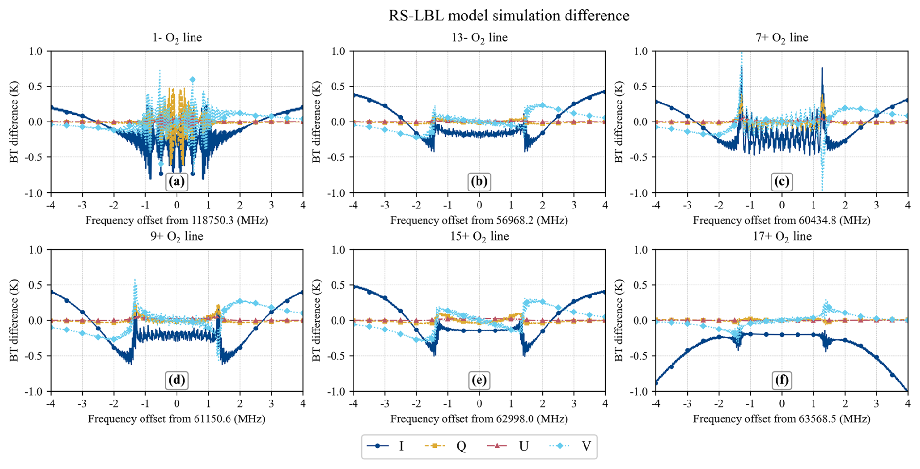
Figure 1 Stokes vector simulation differences between the Hund (b) and Larsson et al. (2019) implementation of the microwave LBL model for total magnetic field strength B_e = 0.5 Gauss, θ = 135°: (a) 1⁻ (118.7503 GHz); (b) 13⁻ (56.9682 GHz); (c) 7⁺ (60.4348 GHz); (d) 9⁺ (61.1506 GHz); (e) 15⁺ (62.9980 GHz); and (f) 17⁺ (63.5685 GHz) line (The dark blue (solid) line represents I, yellow (dashed) line represents Q, red (dashed-dotted) line represents U, and light blue (dotted) lines for V).

3 Oxygen Absorption Line Characteristics

3.1 Model Simulation Differences and Magnetic Field Dependence

The BT matrix and Stokes vector for different oxygen absorption lines based on $g_{J_{\mathrm{N}}}^{\text{Hund\_b}}$ and $g_{J_{\mathrm{N}}}^{\text{Larsson}}$ are calculated using different versions RS-LBL model. The simulations use the 84-layer ECMWF profile dataset developed by Peter Rayer (Met Office) as input, with geomagnetic field parameters obtained from the International Geomagnetic Reference Field (IGRF-13) (Alken et al., 2021). As detailed in Dong et al. (2026), the 7⁺ line exhibits the largest simulation difference, approaching 1 K at a frequency shift of approximately 1.4 MHz, while the 1⁻ line exhibits differences exceeding 0.5 K in the I, Q, and V components within ±2 MHz frequency shift. The U component shows minimal differences across all lines. These simulation differences reflect the combined effects of updating the Zeeman coefficients and oxygen absorption parameters. Figure 1 shows the Stokes parameter differences between the Hund's case (b) and the Larsson et al. (2019) implementations for the selected O₂ lines.

Dong et al. (2026) further investigate the dependence of oxygen absorption lines on magnetic field parameters through two sets of experiments. For the first experiment, cos (θ) is fixed at 0.7 while B_e varies from 0.2 to 0.7 Gauss. In the second, B_e is fixed at 0.45 Gauss while θ varies from 0 to 180°. These results reveal that the 7⁺ line is sensitive to moderate magnetic field strength (0.35–0.55 Gauss), within which left-hand circular and vertical linear polarization exhibit pronounced low-temperature depressions. The 1⁻ line, by contrast, is more sensitive to strong magnetic fields (0.5–0.7 Gauss). Regarding angular dependence, linear polarization brightness temperatures are symmetric about θ = 90°, while left- and right-hand circular polarizations exhibit mirror symmetry. These findings provide a theoretical reference for channel polarization selection.

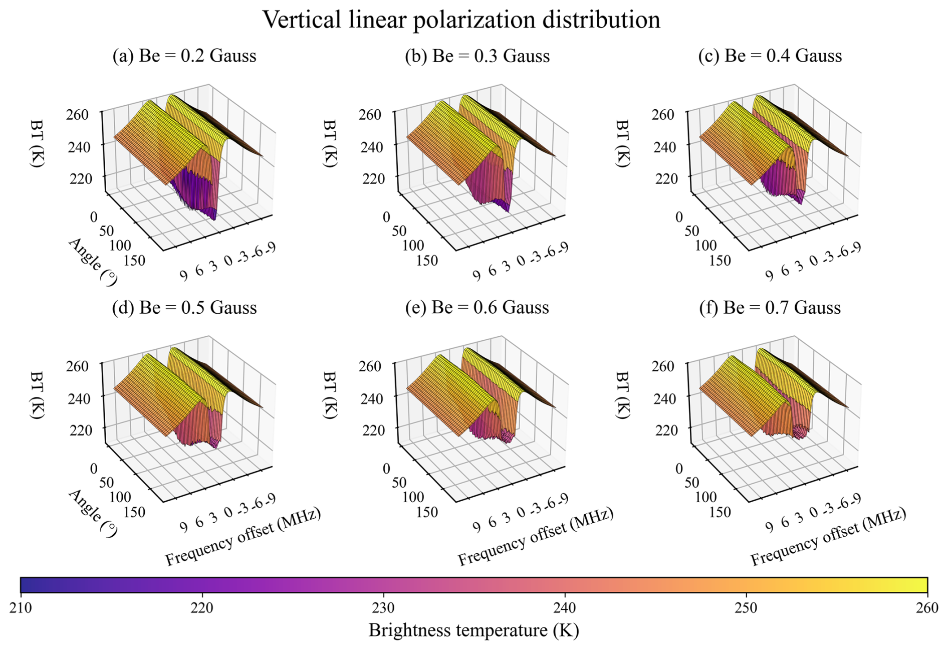
Figure 2 7⁺ line vertical linear polarization simulated brightness temperature distribution at 3 cyclic conditions: frequency shift of oxygen absorption line center from −10 to 10 MHz in steps of 0.1 MHz, B_e ranges from 0.2–0.7 Gauss in steps of 0.1 Gauss, and θ ranges from 0 to 180° in steps of 1°.

3.2 Analysis of Detection Altitude

Most past studies are based on fixed magnetic field strengths or angles, which are not sufficiently representative of the real Earth's atmospheric environment. This section performs three sets of cyclic calculations for B_e, θ, and frequency shift from the O₂ line center: (1) B_e ranges from 0.2–0.7 Gauss with steps of 0.1 Gauss. (2) θ ranges from 0 to 180° in steps of 1°. (3) The frequency is determined by a 10 MHz shift from the O₂ absorption line center in steps of 0.1 MHz. The detection altitude of the 50–70 GHz oxygen absorption line under varying frequency and magnetic field conditions is analyzed, providing theoretical support for designing microwave sounder channels in near space environments. 7⁺ line vertical linear polarization BT is calculated and shown in Fig. 2, since past research focused more on circular polarization.

Each subplot of magnetic field strength in Fig. 2 displays two “peaks” (yellow high-BT) and one “valley” (purple low-BT). From Fig. 2, the “peaks” are primarily located near the 3 MHz frequency shift, with brightness temperatures reaching 260 K, while the “valleys” are mainly around the O₂ line center, with brightness temperatures as low as 220 K. When B_e increases from 0.2 to 0.7 Gauss, the “peaks” pattern remains virtually unchanged, but the low BT regions gradually contract as the magnetic field strength increases. The slope between “peak” and “valley” exhibits distinct temperature gradient variations (e.g., the boundary between yellow and orange), which are nearly unchanged with θ. This phenomenon indicates that the simulated brightness temperature increases with frequency shift and that the BT is unaffected by the observed angle. According to the standard atmospheric temperature profile distribution, the “peak” in Fig. 2 corresponds to an altitude of approximately 1 hPa. The simulated brightness temperature increases initially and then decreases with frequency shift, meaning the detection altitude gradually decreases.

When quantitatively analyzing detection altitude, weighting functions are typically employed, with the peak height corresponding to the altitude where the radiation signal is strongest (Zhang et al., 2024). The WF is typically defined as a function of single-layer (l) atmospheric pressure (P_l) and the transmittance at specific frequencies (ν) (Rosenkranz and Staelin, 1988):

$$\begin{array}{}\text{(10)}& \text{WF}=({\mathrm{\Gamma }}_{l-\mathrm{1}}-{\mathrm{\Gamma }}_{\mathrm{l}})/\left[\ln \right(P_{\mathrm{l}})-\ln (P_{l-\mathrm{1}}\left)\right]\end{array}$$

when l=0 (top of atmosphere):

$$\begin{array}{}\text{(11)}& \text{WF}=(\mathrm{1}-{\mathrm{\Gamma }}_{\mathrm{l}})/\left[\ln \right(P_{l+\mathrm{1}})-\ln (P_{\mathrm{l}}\left)\right]\end{array}$$

The avoidance of linear polarization in near space microwave remote sensing is largely due to its “double-peaked” WF (Rosenkranz and Staelin, 1988). According to Fig. 2, the locations where the WF exhibits “double-peaked” largely correspond to stronger magnetic field strength, meaning that linear polarization introduces uncertainty in observations and simulations of the polar regions or areas prone to electromagnetic storms. However, this “double-peaked” phenomenon changes with frequency shift. When the frequency shift exceeds 2 MHz, the magnetic field strength has a negligible effect on the temperature detection. Furthermore, linear polarization offers significant symmetry advantages at the observed angle. This is important for profiling the near space vertical atmosphere if the same oxygen absorption channel can be used for both linearly and circularly polarized detection.

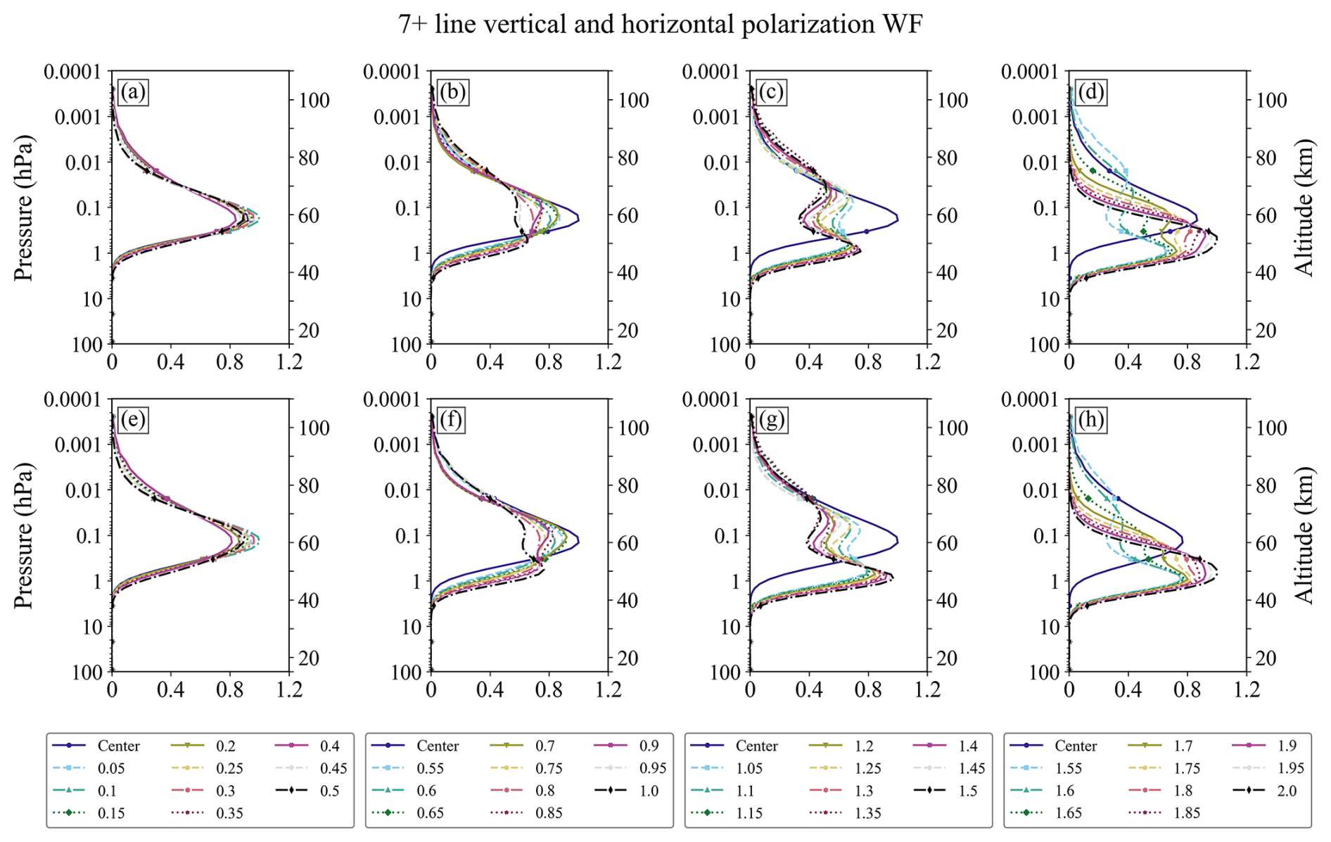
Figure 3 Weighting Functions of 7⁺ line frequency shifts from 0.05–2 MHz at B_e of 0.63 Gauss and cos(θ) of 0.9 for the (a–d) vertical linear polarization, and (e–h) horizontal linear polarization. (a, e) represent frequency shifts of 0.05–0.5 MHz from the 7⁺ line center, (b, f) represent frequency shifts of 0.55–1.0 MHz, (c, g) represent shifts of 1.05–1.5 MHz, (d, h) represent shifts of 1.55–2.0 MHz. Colors denote the frequency offsets, and the curves labelled “Center” correspond to the centre of the 7⁺ line.

To achieve full-polarization near space atmospheric detection, it is essential to investigate the distribution characteristics of the “double-peak” weighting function in linear polarization. The “double-peak” WF is more likely to appear at strong B_e (Fig. 2). Therefore, this study fixed the magnetic field strength and cos(θ) at 0.63 Gauss and 0.9, respectively. The fine-structure weighting function for the 7⁺ (60.4348 GHz) line and its 2 MHz frequency shift in 0.05 MHz is shown in Fig. 3. From Fig. 3, the WF is relatively narrow when the 7⁺ line frequency shift is within 0.5 MHz, and the peak heights for both vertical and horizontal polarization are approximately 60 km (0.1 hPa). The weighting function starts to broaden at frequency shift 0.75 MHz, gradually exhibiting “double-peaked”. The altitudes of “double-peaked” are approximately 50 and 65 km, with the lower-level signal being stronger, particularly in horizontal polarization. The “double-peak” structure gradually weakens as the frequency shift continues to increase, and the WF signal of the lower atmosphere gradually intensifies. At a frequency shift of 2 MHz, it exhibits a perfect narrow “single-peaked” WF.

Therefore, for linear polarization, oxygen line frequency shifts outside the range of 0.8–1.8 MHz can be selected to avoid the effects of the “double peak”. This selection of extreme cases aims to enable detailed simulation and analysis of oxygen lines under strong magnetic field conditions. In reality, not all oxygen absorption lines exhibit a “double peak” (such as 17⁺) at high magnetic field strengths, which also depends on the intensity of the oxygen absorption line itself. In actual detection, multiple oxygen absorption lines are typically combined to diminish the influence of a single line.

4 Microwave Sounder in Near Space

4.1 SSMIS UAS Channel Characteristics

The SSMIS on board DMSP satellites features six channels capable of detecting altitudes from 20 to 100 km (Swadley et al., 2008). To achieve upper atmospheric detection, a narrow bandwidth is currently the preferred method (Lipton, 2003). However, a single narrow bandwidth often comes with significant channel noise, which may render the data unusable. The relationship between channel noise and bandwidth is as follows (Zhang et al., 2024):

$$\begin{array}{}\text{(12)}& \text{NEDT}=(T_{\mathrm{r}}+T_{\mathrm{a}})/\sqrt{\text{BW}\cdot t}\end{array}$$

where NEDT denotes the channel noise equivalent delta temperature (unit: K), BW represents the total effective bandwidth of the contributing passbands (unit: Hz), T_r is the receiver equivalent noise temperature (unit: K), T_a is the antenna temperature (unit: K), and t is the integration time (unit: s).

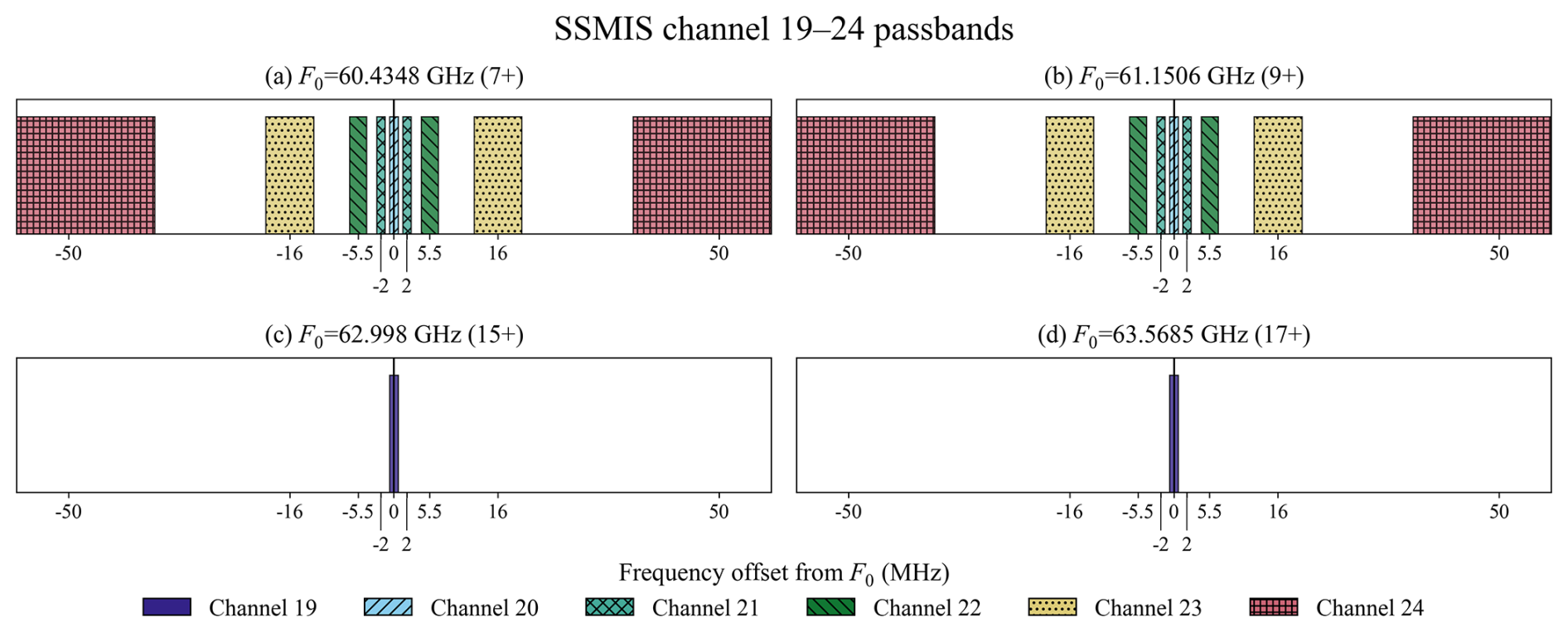
Figure 4 SSMIS channel 20–24 (upper panel) and channel 19 (bottom panel) passband distribution. The x-axis labels the passband frequency shift from the O₂ line, while the “rectangular” width indicates the bandwidth.

Figure 5 HMAS all-channel passband distribution.

To reduce noise, channels are typically designed as a double- or quadruple-sideband, and multi-line cooperative detection can significantly improve NEDT performance (Kunkee et al., 2008; Pardo et al., 1998). In SSMIS channel 19, the local oscillator (LO) is positioned between the 15⁺ and 17⁺ line frequencies, while channels 20–24 are between the 7⁺ and 9⁺ lines to achieve multiband detection. These UAS channels are designed for circular polarization. The SSMIS channel passband distribution is shown in Fig. 4. SSMIS channel 20 has two passbands with bandwidths of approximately 1.35 MHz covering the 7⁺ and 9⁺ lines, respectively. Channel 19 also features two passbands with bandwidths of approximately 1.35 MHz, covering the 15⁺ and 17⁺ lines, respectively. Channel 21 has four passbands, each with a bandwidth of approximately 1.3 MHz, positioned 2 MHz on either side of the 7⁺ and 9⁺ oxygen absorption lines. Channels 22–24 also feature four passbands centered at the 7⁺ and 9⁺ oxygen line frequencies, with frequency shifts of ±5.5, ±16, and ±50 MHz, respectively. Their respective bandwidths are 2.6, 7.35, and 26.5 MHz. The detection altitude of the channel decreases as the oxygen line shift increases, enabling detection of near space environments (Swadley et al., 2008).

4.2 HMAS Passband Distribution

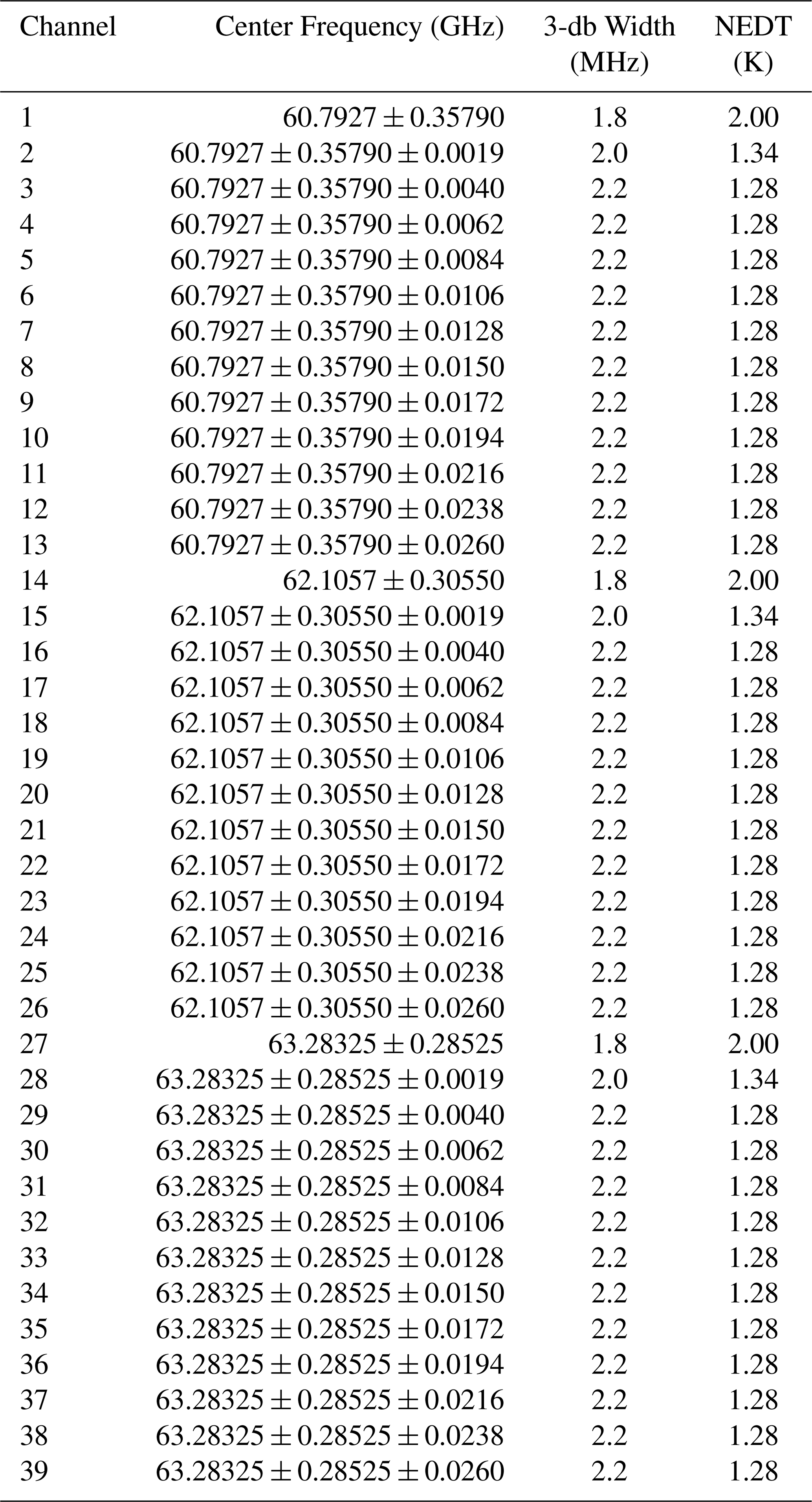
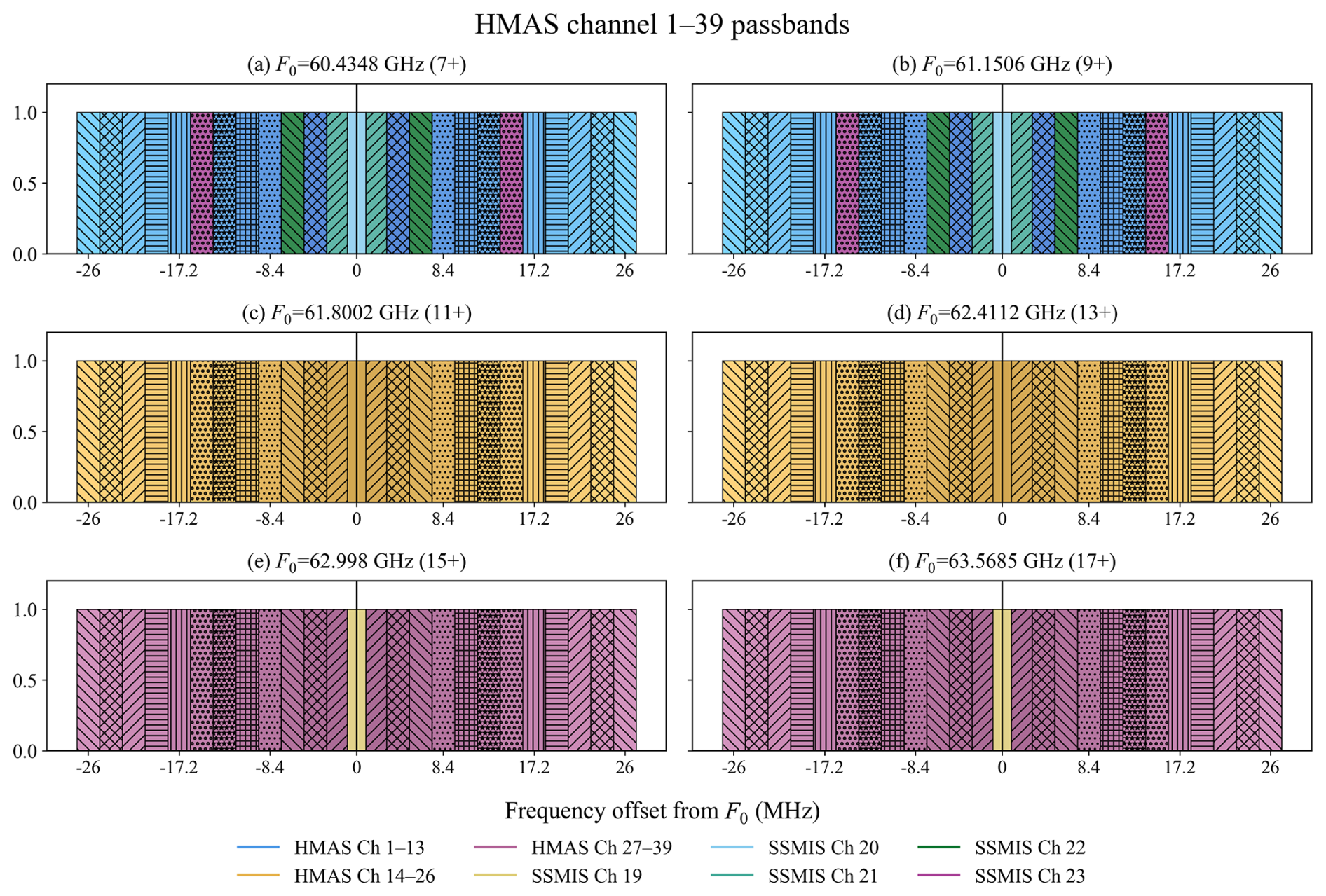
The SSMIS is relatively mature, with remaining instruments approaching the end of their operational lifetimes. This study proposes a high-resolution microwave sounder based on the same design principles as SSMIS, but with linear polarization, aiming to increase near space observations, with the new channels complementing and extending the existing SSMIS UAS channels. To achieve high-resolution continuous detection, this study introduces channels that utilize new oxygen line combinations around 11⁺ and 13⁺ based on the existing channel specifications. The first channel bandwidth centered on each oxygen line is set to 1.8 MHz to reduce channel noise. Then a second channel with a bandwidth of 2 MHz is set near each further oxygen line offset of 1.9 MHz. Thanks to recent microwave hyperspectral detection technology, the channels away from the absorption line centers can all be set to narrow values, so the bandwidths of the remaining channels are all set to 2.2 MHz.

Based on these design principles, multiple channels with narrow bandwidth can be formed on either side of the 7⁺, 9⁺, 11⁺, 13⁺, 15⁺, and 17⁺ oxygen lines. All these channels, covering both sides of the oxygen absorption lines, can theoretically be implemented on the same instrument named Hyperspectral Microwave Atmospheric Sounder (HMAS). Figure 5 shows part of the HMAS channel distribution, where the top panel, middle panel, and bottom panel groups represent three sets of detection channels designed with different oxygen line combinations, with the corresponding passbands for the SSMIS channels overlaid. From Fig. 5, approximately 150 channels of the HMAS achieve continuous frequency coverage within the 7⁺, 9⁺, 11⁺, 13⁺, 15⁺, and 17⁺ oxygen line offsets to ±26 MHz with detection frequency from about 60–63 GHz.

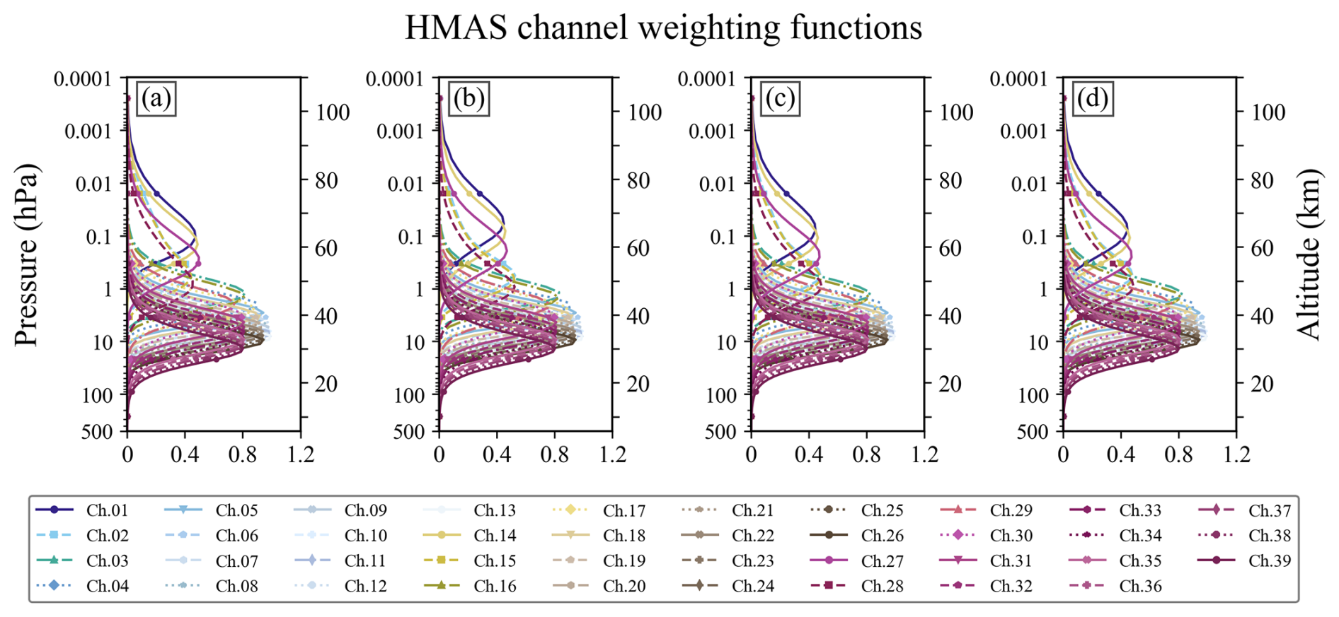
Figure 6 HMAS channel Weighting Functions (WF) for the (a) vertical-, (b) horizontal-, (c) right-, and (d) left-polarization. The first three channels in each group (channels 1–3, 14–16, and 27–29) are highlighted from the same color family.

To compare with SSMIS, the HMAS 150 channels are set to passband and combined into 39 composite channels. In HMAS 39 composite channels, there are 3 double-sideband and 36 quadruple-sideband composite channels. For microwave radiometers, the T_a is typically assumed to be 290 K, and the T_r is calculated based on frequency, approximately 300 K at 60 GHz (Zhang et al., 2024). In this study, the system noise temperature is assumed to be T_r+T_a = 800 K. To reduce channel noise, the integration time is extended to approximately 44.3 ms. This can be achieved through software averaging (i.e., accumulating and averaging observations from the same channel over multiple scan cycles), which is within the allowable range of satellite scan periods. According to Eq. (12), the NEDT of HMAS Composite Channel 1 is approximately 2 K. Table 1 gives the HMAS channel parameters.

The integration time for the SSMIS channel 19–23 is 25.2 ms, and for channel 24 is 12.6 ms, which are fixed hardware parameters determined by the radiometer design (Swadley et al., 2008). For comparison, the system noise is also set to 800 K when calculating the NEDT for SSMIS in this study. From Eq. (12), the SSMIS Channels 19–20 NEDT is approximately 3 K, which is highly consistent with the reported (2.7 K) (Kunkee et al., 2008). The number of channels and vertical resolution in this study are significantly higher than those of SSMIS, allowing for an appropriate extension of the integration time.

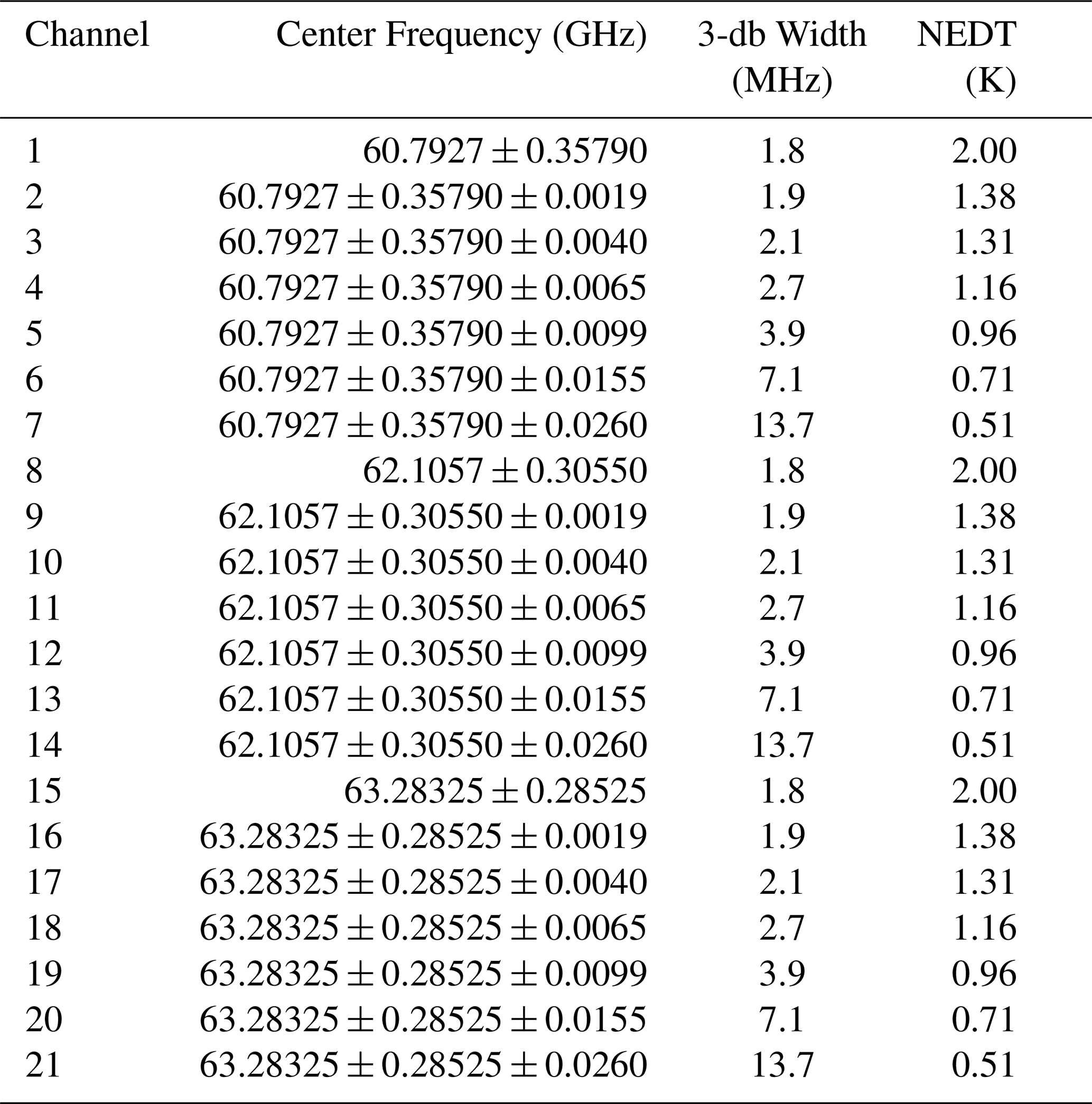
Based on the same principle, high-resolution channels that do not utilize microwave hyperspectral detection technology are also proposed in this study for a conventional Microwave Atmospheric Sounder (MAS). The MAS and HMAS use the same three oxygen absorption line combinations but differ mainly in channel bandwidths and channel numbers away from the absorption line centers. The MAS uses progressively broader channels, while the HMAS uses more narrow channels to provide finer frequency sampling. A double-sideband channel with a bandwidth of 1.8 MHz was set covering the oxygen absorption line. Six quadruple-sideband channels were established at frequencies progressively shifting away from the absorption line center: 1.9, 4.0, 6.5, 9.9, 15.5, and 26 MHz, with respective bandwidths of 1.9, 2.1, 2.7, 3.9, 7.1, and 13.7 MHz. Table 2 gives the MAS channel parameters suitable for conventional detection techniques. This is essentially an extension of SSMIS channels 19–23, incorporating the 11⁺ and 13⁺ lines. However, the most significant difference between MAS and SSMIS is its capability to perform linear or circular polarization detection. The MAS can be manufactured with reference to the structure of ATMS or AMSU to achieve end-to-end calibration.

Figure 7 As Fig. 6, but for SSMIS channel 19–24.

4.3 Comparison of SSMIS and HMAS Channel Simulations

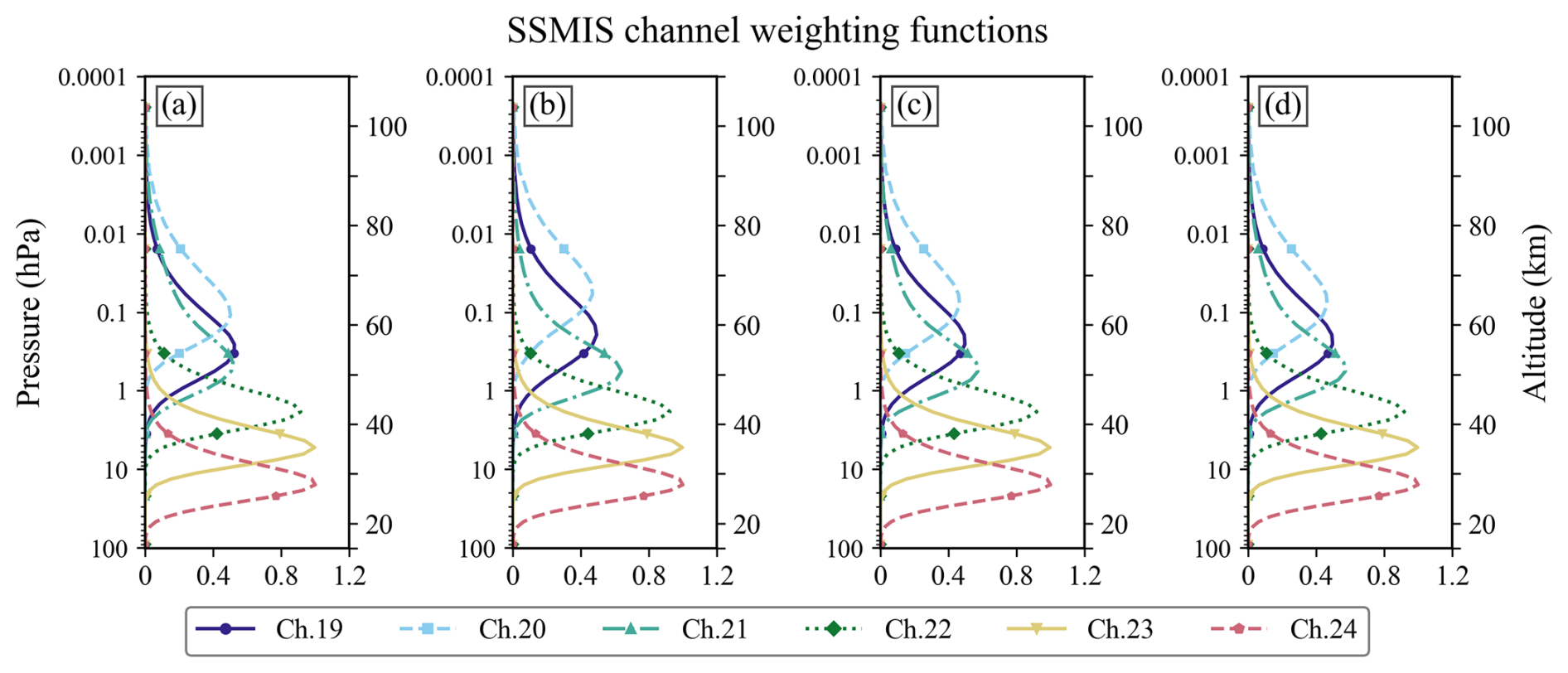
The atmospheric profile dataset and RS-LBL model configuration used for SSMIS and HMAS simulation follow the same setup as described in Dong et al. (2026, Sect. 2). The atmospheric profile dataset was developed by Peter Rayer (Met Office). It consists of 13 495 randomly sampled model profiles from the European Centre for Medium-Range Weather Forecasts (ECMWF), providing high vertical resolution (extending up to 0.0002 hPa). The key characteristics required for upper atmospheric simulations can be met by utilizing the average of this profile dataset. Figure 6 shows the HMAS weighting function distribution for different polarizations. The HMAS channels are grouped into three sets based on oxygen absorption line combinations: Group 1 (blue) comprises channels 1–13 centered around the 7⁺ and 9⁺ lines, Group 2 (yellow) includes channels 14–26 centered around the 11⁺ and 13⁺ lines, and Group 3 (pink) consists of channels 27–39 centered around the 15⁺ and 17⁺ lines. From Fig. 6, it is shown that the three double-sideband channels covering the respective oxygen absorption lines exhibit the highest peak among all WFs. Detection height gradually decreases as the passband moves further from the oxygen line center, with every 13 channels exhibiting a similar pattern. Using only channels 1–2, 14–15, and 27–28 enables detection at upper altitudes of approximately 40–80 km, while the remaining channels complete the high-resolution coverage of about 20–55 km.

The SSMIS UAS channel WFs are shown in Fig. 7 for different polarizations. The six-channel weighting functions also achieve similar coverage to HMAS from 100 to 0.001 hPa. The SSMIS channel 24, with a center frequency shift of about 50 MHz, has a WF peak height of approximately 28 km (16 hPa). In contrast to SSMIS, the HMAS high-density weighting function is expected to provide richer atmospheric information in the near space.

To further validate the physical consistency of the HMAS channel design, the BT simulations of HMAS composite channels and SSMIS UAS channels are compared using the Advanced Radiative Transfer Modeling System (ARMS) developed based on the RS-LBL model with Larsson implementation. The simulations are performed using the SABER V2.0 temperature profiles as input, with the IGRF-13 geomagnetic field model providing the magnetic field parameters. The HMAS composite channels are constructed by combining the original 150 hyperspectral channels into 39 composite channels, with the central frequency and bandwidth of each composite channel designed to match the detection altitude characteristics of the corresponding SSMIS channels.

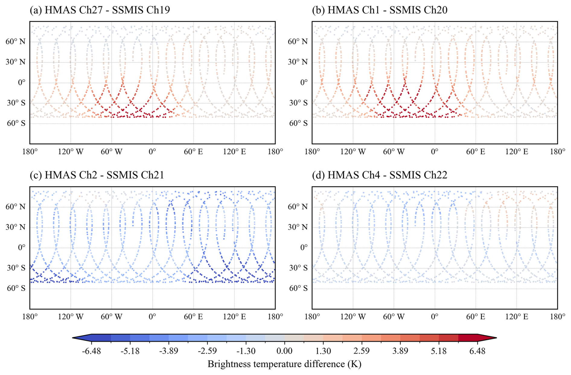
Figure 8 Global brightness temperature differences distribution between HMAS and SSMIS corresponding channels on 1 January 2024 for (a) HMAS composite channel 27 and SSMIS channel 19, (b) HMAS composite channel 1 and SSMIS channel 20, (c) HMAS composite channel 2 and SSMIS channel 21, and (d) HMAS composite channel 4 and SSMIS channel 22.

Figure 8 presents the global distribution of BT differences between HMAS composite channels and SSMIS channels on 1 January 2024. Four representative channel pairs are selected for comparison: (a) HMAS composite channel 27 and SSMIS channel 19, (b) HMAS composite channel 1 and SSMIS channel 20, (c) HMAS composite channel 2 and SSMIS channel 21, and (d) HMAS composite channel 4 and SSMIS channel 22.

The BT differences exhibit distinct spatial patterns that vary across channel pairs, reflecting the combined influence of geomagnetic field strength and latitude. For HMAS composite channels 27 and 1, which correspond to SSMIS channels 19 and 20, the BT differences are smaller at high latitudes where the geomagnetic field is stronger, typically within ±1.3 K, while at low latitudes, the differences become larger, reaching up to 6 K. In contrast, HMAS composite channel 2 (corresponding to SSMIS channel 21) displays the opposite behavior: larger BT differences, up to −6 K, are observed at higher geomagnetic field strength. For HMAS composite channel 4 (corresponding to SSMIS channel 22), the BT differences exhibit a predominantly latitudinal dependence rather than a magnetic field dependence.

These contrasting patterns can be attributed to subtle differences in center frequency and bandwidth between the HMAS composite channels and their SSMIS counterparts, leading to shifts in the weighting function peak altitude. Since the Zeeman splitting effect varies with both magnetic field strength and atmospheric pressure (altitude), channels with different effective detection heights sample different layers of the atmosphere, where the temperature profile and its sensitivity to magnetic field perturbations differ. Consequently, the BT difference between HMAS and SSMIS at a given location is not solely determined by the local geomagnetic field intensity but also by the vertical alignment of their respective weighting functions. This explains why some channel pairs show larger differences in strong-field regions (channel 2 vs. 21), while others show smaller differences under the same conditions (channels 1 and 27 vs. 19 and 20), and why channel 4 vs. 22 exhibits a primarily latitudinal pattern governed by the background temperature gradient rather than magnetic field variations.

Figure 9 As Fig. 8, but for 1 August 2024.

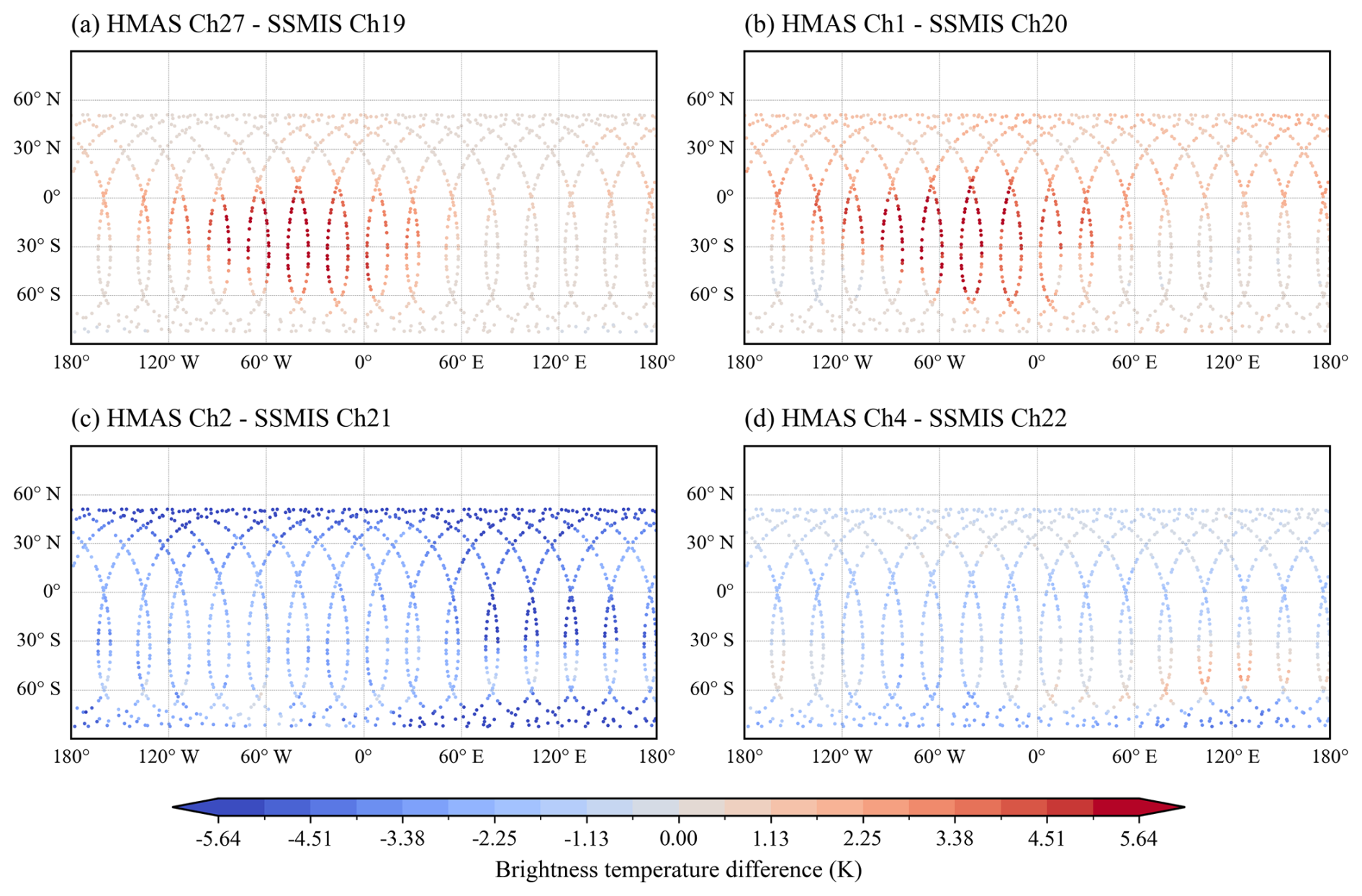
Figure 9 presents the corresponding BT difference distribution on 1 August 2024. The overall spatial pattern of BT differences is similar to that in January, with the differences remaining generally within ±1.13 K across most latitude bands. However, notable seasonal variations are evident, particularly in the polar regions, where the BT differences exhibit asymmetry between the Northern and Southern Hemispheres. This asymmetry is partly attributable to the SABER yaw cycle: the SABER has a yaw cycle of approximately two months (60 d), causing its observation region to alternate between 53° S–83° N and 83° S–53° N every two months (Dong et al., 2026). Consequently, the sampling coverage of SABER temperature profiles used for BT simulation differs between January and August.

Among the four channel pairs, HMAS composite channel 4 (corresponding to SSMIS channel 22) exhibits the most pronounced seasonal variation. This channel pair has the largest frequency offset from the oxygen absorption line center among the four comparisons, corresponding to a lower WF peak altitude. At this altitude, the atmospheric temperature exhibits stronger seasonal variability compared to the upper stratosphere and mesosphere, where the other three channel pairs are primarily sensitive. The larger seasonal temperature contrast between winter and summer at lower altitudes amplifies the BT difference between January and August for this channel pair. In contrast, HMAS composite channels 27, 1, and 2 (corresponding to SSMIS channels 19, 20, and 21) have weighting function peaks at higher altitudes, where the seasonal temperature variation is relatively weaker.

The BT differences between HMAS and SSMIS depend on the channel parameter design, with local differences reaching approximately 6 K. The comparisons show broadly similar sounding characteristics, together with channel-dependent differences across the two seasons.

4.4 Comparison of SSMIS and HMAS Temperature Profile Retrieval Results

To further validate the rationality of the HMAS channel design, a temperature profile retrieval experiment is conducted using an improved BP neural network algorithm. The experiment consists of three steps: brightness temperature forward simulation, retrieval model training, and retrieval accuracy evaluation, with consistent input profiles, radiative transfer model, retrieval algorithm, and evaluation criteria applied to both HMAS and SSMIS channels.

The retrieval experiment adopts a hybrid approach combining physical forward modeling with data-driven inversion. The ARMS with the Zeeman module is used to generate simulated BT datasets for both SSMIS channels 19–24 and all HMAS channels. This forward model is rigorously based on radiative transfer theory and the Zeeman splitting physical mechanism, ensuring the physical reliability of the input data. The improved BP neural network then performs the nonlinear mapping from BT to temperature profiles, leveraging the efficiency of machine learning for high-dimensional data fitting. This approach combines the physical constraints of radiative transfer with the efficiency of machine learning.

The experiment period is set to the year 2024. SABER V2.0 temperature profiles from three groups of dates (1st–5th, 11th–15th, and 24th–25th of each month) are selected to ensure comprehensive coverage of atmospheric temperature characteristics across different seasons. SABER profiles are used as the truth reference due to their high vertical resolution and reliable quality. To facilitate subsequent retrieval and statistical comparison, SABER data from 100 to 0.001 hPa are selected based on the weighting function peak altitudes of SSMIS channels 19–24 and all HMAS channels, forming a unified 200-layer atmospheric temperature profile dataset. The SABER temperature profiles and IGRF-13 geomagnetic field parameters are then input into the ARMS model with the Zeeman module to simulate BTs for SSMIS and HMAS channels, respectively. A total of 144 d of simulated BT datasets are constructed for both instruments.

The retrieval algorithm and procedure are strictly controlled to eliminate retrieval errors caused by differences in algorithms or non-instrument channel parameters. The improved BP neural network is trained using 120 d of simulated BT data and corresponding SABER temperature profiles (1st–5th and 11th–15th of each month in 2024). The remaining 24 d (24th–25th of each month) serve as an independent test set. The SSMIS channel 19–24 and HMAS full-channel simulated BTs from these test dates are input into the trained retrieval model to obtain temperature profiles, which are then compared with the corresponding SABER profiles for validation.

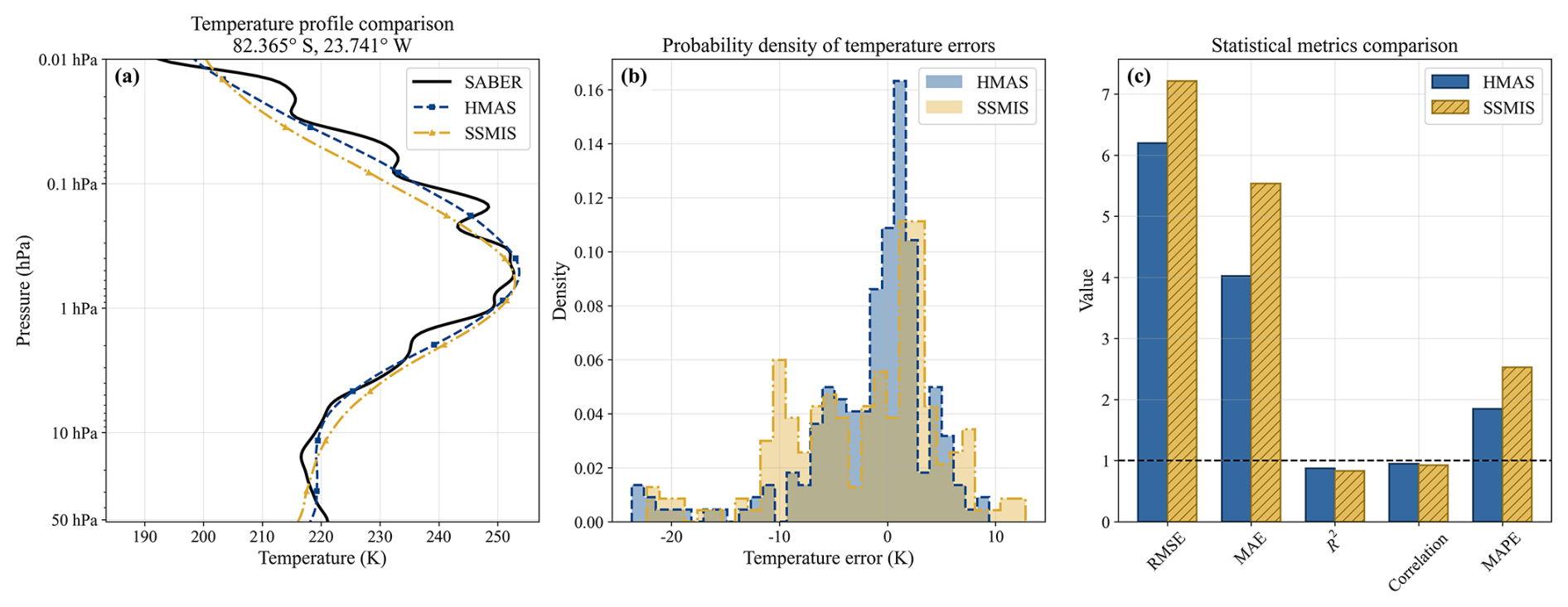
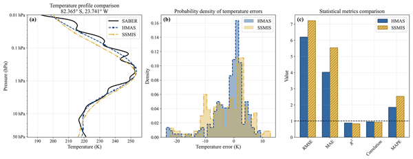
Figure 10 Comparison of the retrieved temperature profile (No. 41) based on HMAS and SSMIS channel simulations with the SABER temperature profile on 24 March 2024: (a) vertical distribution of atmospheric temperature from 50 to 0.01 hPa for the SABER profile (black solid line), the HMAS-based retrieval result (blue dashed line), and the SSMIS-based retrieval result (yellow dash-dotted line), (b) probability density function (PDF) of retrieval errors relative to the SABER profile for HMAS (blue) and SSMIS (yellow), (c) statistical comparison of root mean square error (RMSE), mean absolute error (MAE), coefficient of determination (R²), correlation coefficient, and mean absolute percentage error (MAPE) for HMAS and SSMIS retrieval results.

The improved BP neural network incorporates several key enhancements tailored to the characteristics of HMAS channels. In terms of input features, in addition to the channel BTs, two types of auxiliary information are included: statistical features of channel BTs (mean, standard deviation, and range) to capture the intrinsic relationships between different channel observations, and sine-cosine encoded latitude and longitude features to enable the model to learn the latitudinal distribution characteristics of atmospheric temperature. In the network architecture, a dual residual block structure is adopted to mitigate the gradient vanishing problem in deep networks, thereby accelerating convergence and improving training stability. A squeeze-and-excitation (SE) channel attention module is also introduced, which automatically learns the dependencies between different channels and generates adaptive weight coefficients, allowing the model to identify channels that contribute more significantly to temperature retrieval while suppressing redundant or noisy channels. For the loss function, a layer-weighted mean squared error is designed, dividing the 200-layer temperature profile into lower, middle, and upper altitude intervals with different weight coefficients. Higher weights are assigned to the 50–0.01 hPa, which is the primary focus of this study.

Data augmentation is applied to improve model robustness. Gaussian noise of 1–2 K is added to the simulated BTs to simulate instrument noise and measurement errors in actual observations. Random channel masking is also applied to simulate scenarios where some channels may fail during operation. The AdamW optimizer with cosine annealing warm restarts learning rate scheduling is used for training, and an early stopping strategy is implemented to prevent overfitting.

Figure 10 presents the retrieval results for a randomly selected temperature profile (No. 41) on 24 March 2024, compared with the SABER truth profile. Figure 10a shows the vertical distribution of atmospheric temperature from 50 to 0.01 hPa, where the black solid line represents the SABER observation, the blue dashed line represents the HMAS retrieval, and the yellow dash-dotted line represents the SSMIS retrieval. The HMAS retrieval shows better agreement with the SABER profile, while the SSMIS retrieval exhibits larger deviations near 10–5 and 0.1 hPa. Figure 10b displays the probability density function (PDF) of retrieval errors for both instruments. The HMAS retrieval errors are more concentrated within ±2 K compared to SSMIS, indicating a lower probability of large errors. Figure 10c quantifies the retrieval performance using five core metrics. The results show that the root mean square error (RMSE), mean absolute error (MAE), and mean absolute percentage error (MAPE) of HMAS retrievals are significantly lower than those of SSMIS, while the coefficient of determination (R²) and correlation coefficient of HMAS are closer to 1, demonstrating superior retrieval accuracy.

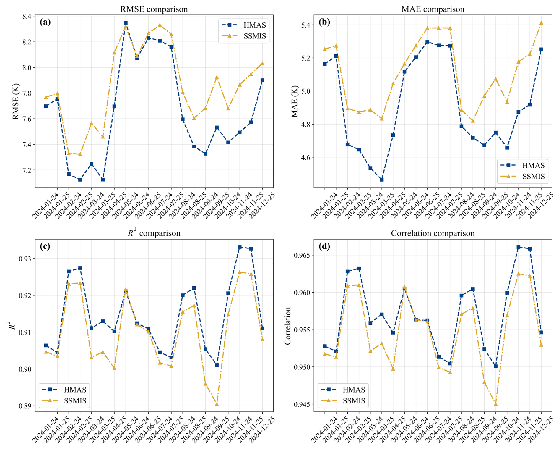
Figure 11 Daily mean statistics of all retrieved profiles for 20 available dates falling on the 24th or 25th of the month between January and December 2024, for HMAS (blue dashed line) and SSMIS (yellow dash-dotted line): (a) RMSE, (b) MAE, (c) R², and (d) correlation coefficient.

Considering the limitations of single-day analysis, the daily mean statistics of all retrieved profiles on the 24th and 25th of each month from January to December 2024 are further analyzed, as shown in Fig. 11. The blue dashed and yellow dash-dotted lines represent the HMAS and SSMIS results, respectively. From the RMSE time series (Fig. 11a), except for 25 April 2024, when the HMAS RMSE is slightly higher than that of SSMIS, the HMAS RMSE is consistently lower for all other dates, indicating that the HMAS retrievals are generally closer to the true values. The MAE time series (Fig. 11b) shows that the HMAS MAE remains lower than that of SSMIS throughout the entire experimental period. The R² comparison (Fig. 11c) shows that both instruments achieve R² values above 0.8, confirming the overall effectiveness of the retrieval algorithm. Except for three dates (25 April, 24 May, and 24 June 2024), the HMAS R² is consistently closer to 1. The correlation coefficient trends (Fig. 11d) are consistent with the R² results, further validating the retrieval accuracy advantage of HMAS.

Table 3 Statistical comparison of HMAS and SSMIS temperature profile retrieval results.

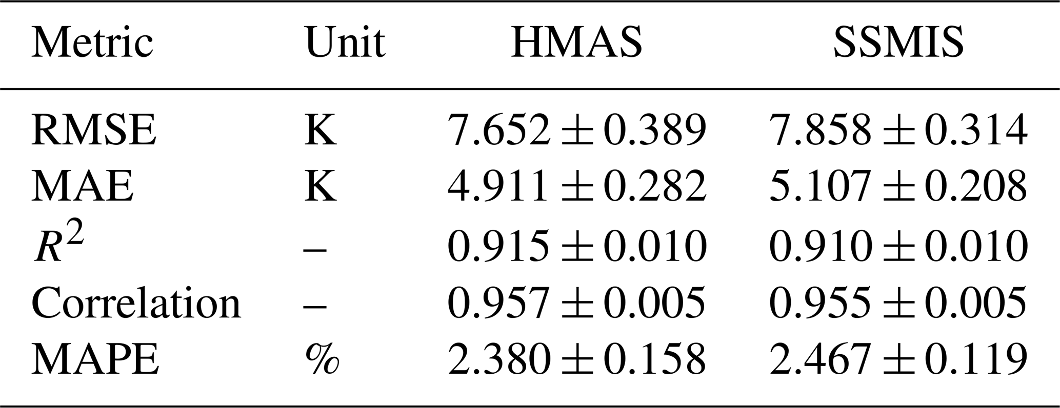
To comprehensively evaluate the overall retrieval performance of both instruments, the five metrics are statistically summarized for all retrieved profiles throughout the experiment period, as shown in Table 3. The results demonstrate that HMAS outperforms SSMIS across all evaluation metrics: HMAS achieves an RMSE of 7.652 ± 0.389 K compared to 7.858 ± 0.314 K for SSMIS, an MAE of 4.911 ± 0.282 K compared to 5.107 ± 0.208 K, an R² of 0.915 ± 0.010 compared to 0.910 ± 0.010, a correlation coefficient of 0.957 ± 0.005 compared to 0.955 ± 0.005, and a MAPE of 2.380 ± 0.158 % compared to 2.467 ± 0.119 %. These results are consistent with the theoretical expectations for HMAS channels, where the greater number of detection channels provides richer atmospheric state information, thereby enabling higher retrieval accuracy.

5 Conclusions

The Special Sensor Microwave Imager Sounder (SSMIS) has six upper atmospheric sounding (UAS) channels that have demonstrated positive impacts on data assimilation (Hoppel et al., 2013). This study proposes both conventional and hyperspectral linearly polarization channels parameters based on the simulation and analysis of oxygen absorption lines, aiming to complement and extend the capability of existing SSMIS observations, particularly as it reaches the end of its life. The channel configurations for both the hyperspectral HMAS and the conventional MAS are comparable to SSMIS, featuring double-sideband covering the oxygen line and quadruple-sideband channels on either side of the oxygen absorption line. To reduce channel noise, the bandwidth covering oxygen lines has been appropriately broadened. The HMAS comprises 150 original channels covering the 60–63 GHz, optimized to 39 composite channels, while the MAS provides 21 channels as a conventional alternative. The detection altitude characteristics of oxygen absorption lines under varying frequency shifts and magnetic field conditions are systematically analyzed. The results indicate that the O₂ line center and frequency shift within 2 MHz are highly sensitive to magnetic field strength (B_e), particularly when it exceeds 0.4 Gauss, but above 2 MHz, there is negligible sensitivity. The weighting function analysis reveals that the “double-peaked” phenomenon in linear polarization is primarily associated with frequency shifts within the 0.8–1.8 MHz range under strong magnetic field conditions, providing guidance for channel frequency selection in linear polarization detection.

The SSMIS and HMAS composite channel weighting function distributions are compared. Overall, both the SSMIS and HMAS WFs achieve coverage from 50 to 0.01 hPa, but HMAS has a higher density. Using only HMAS channels 1–2, 14–15, and 27–28 enables detection at upper altitudes of approximately 40–80 km, while the remaining channels complete the high-resolution coverage of about 20–55 km. The HMAS channel parameters are further validated through brightness temperature simulations using the ARMS model developed based on the RS-LBL model with Larsson et al. (2019) implementation. The global distribution of BT differences between HMAS composite channels and SSMIS channels on representative dates in January and August 2024 shows that the differences are generally within ±1.3 K across most latitude bands, with larger differences in some regions depending on the channel parameters. This confirms the physical consistency of the HMAS channel design with the well-validated SSMIS upper atmospheric sounding (UAS) channels.

Temperature profile retrieval experiments using an improved back propagation (BP) neural network with dual residual blocks and squeeze-and-excitation (SE) attention mechanism are conducted based on 144 d of simulated BT data in 2024. The retrieval results demonstrate that HMAS channels achieve superior accuracy (RMSE: 7.652 ± 0.389 K, MAE: 4.911 ± 0.282 K, R²: 0.915 ± 0.010) compared to SSMIS channels 19–24 (RMSE: 7.858 ± 0.314 K, MAE: 5.107 ± 0.208 K, R²: 0.910 ± 0.010), with the HMAS retrieval errors more concentrated within ±2 K. The daily mean statistics from January to December 2024 further confirm that HMAS generally outperforms SSMIS across all evaluation metrics, indicating that the greater number of detection channels provides richer atmospheric state information and enables higher retrieval accuracy.

This study focuses on the HMAS 150 channels at 60–63 GHz, while additional channel configurations at other frequency bands remain to be investigated. The current HMAS channel configuration is a conservative adaptation of existing techniques. In the future, channel setups can be fully adjusted based on technological capabilities, though all configurations require detailed simulation and analysis of the O₂ fine-structure lines. The temperature profile retrieval framework developed in this study can also be applied to compare the performance of HMAS, MAS, and SSMIS channel configurations.