UAV-based method for measuring CO₂ emissions in forest ecosystems

This study addresses the difficulty of accurately quantifying CO₂ emissions in forest ecosystems due to spatial heterogeneity, complex terrain, and the combined effects of horizontal and vertical transport. A methodology for quantifying 3-D CO₂ emissions using an unmanned aerial vehicle was developed, evaluated, and applied to a forest ecosystem. The measurement platform was integrated with a high-precision closed-path CO₂ analyzer to measure CO₂ mole fractions and a calibrated ultrasonic anemometer to measure wind vectors, together with profile measurements of temperature and pressure. Within a mass-balance framework, the instrumented platform was flown along horizontal loops at multiple heights together with vertical ascent flight tracks, acquiring data along the flight tracks that were used to quantify horizontal advective and vertical turbulent carbon dioxide emission components, respectively. The method was applied at a subtropical plantation forest and evaluated against fluxes derived using a nearby eddy covariance flux tower. Validation against long-term CO₂ flux measurements from the permanently installed eddy covariance system shows that vertical CO₂ fluxes derived from the airborne observations agree well with the tower observations across seasons, with a correlation coefficient of 0.9 based on 168 paired flux estimates collected between May 2023 and December 2024. Measurements collected along the horizontal box-pattern flight paths further reveal diurnal variations in local canopy-air CO₂ mass transport: lateral advection dominates in the early morning, whereas vertical uptake prevails under well-mixed midday conditions. Sensitivity analysis of emission intensities across control volumes with different horizontal dimensions (50 × 50, 100 × 100, and 150 × 150 m²) and a constant vertical extent of 50 m revealed stronger scale dependence during autumn mornings, indicating significant spatial heterogeneity in CO₂ emissions. Uncertainty assessment suggests that the total relative uncertainty of the emission estimates derived using this approach is typically approximately 30 %, with wind-field measurement as the main error source. Overall, the proposed approach provides a flexible and reliable method for analyzing near-surface 3-D CO₂ transport over structurally heterogeneous forests and complex terrain, helping to overcome the limited spatial coverage of traditional flux towers and remote sensing.

1 Introduction

Carbon dioxide (CO₂) is the dominant anthropogenic greenhouse gas in the atmosphere, contributing approximately 50 %–60 % to the enhanced greenhouse effect excluding water vapor (WMO, 2023). The atmospheric CO₂ budget is strongly impacted by biospheric carbon cycles. Forest ecosystems, in particular, play a critical role in the terrestrial carbon cycle and are widely recognized as major carbon sinks, covering about 40 % of the global land surface and representing some of the most extensive and structurally complex ecosystems on Earth (Bonan, 2008; IPCC, 2021; Pan et al., 2011). Accurate quantification of forest-atmosphere carbon exchange remains essential for constraining regional and global carbon budgets and for evaluating ecosystem feedbacks from climate change. Recent synthesis studies and observation-network analyses continue to highlight the importance of improving carbon flux measurements across heterogeneous ecosystems (Fang et al., 2024; Burman et al., 2025). However, despite decades of carbon-cycle research using a range of observational platforms, including stationary towers, satellites, and manned aircraft (Baldocchi, 2003; Gioli et al., 2004; Jung et al., 2020), commonly applied flux quantification methods often resolve only selected components of 3-D CO₂ transport. For example, eddy covariance (EC) methods quantify vertical turbulent exchange (Baldocchi, 2003), whereas aircraft-based mass-balance approaches commonly quantify emissions from horizontal advective transport across control volume boundaries (Cambaliza et al., 2014; Gordon et al., 2015). In forest ecosystems, strong spatial heterogeneity, complex canopy-atmosphere interactions, and non-negligible horizontal transport processes can introduce substantial uncertainties into quantitative estimates of ecosystem-atmosphere CO₂ exchange (Baldocchi, 2008; Schimel et al., 2015). Although vertical CO₂ flux is the primary quantity used to evaluate forest-atmosphere carbon exchange, horizontal advection can also contribute to the local CO₂ mass balance above the canopy. Under weakly mixed conditions, suppressed vertical turbulent transport can lead to CO₂ accumulation within and below the canopy, while terrain-induced drainage flows and spatial heterogeneity can promote lateral transport and generate horizontal CO₂ gradients. Consequently, horizontal advective convergence or divergence can contribute to the local CO₂ mass balance, such that vertical turbulent flux measured at a single tower may not fully represent the local ecosystem-atmosphere exchange (Aubinet et al., 2002; Feigenwinter et al., 2004; Leuning et al., 2008). Measurements that characterize lateral CO₂ transport across finite control volume boundaries are therefore useful for diagnosing when the assumption of horizontal homogeneity is valid and when local advection may influence the spatial representativeness of vertical flux measurements. As a result, flux measurement and quantification approaches capable of resolving both horizontal and vertical CO₂ transport are required.

The EC flux measurement technique is a widely used method (Aubinet et al., 2012; Baldocchi, 2003; Burman et al., 2025; Pastorello et al., 2020; Fang et al., 2024) for quantifying ecosystem-scale vertical CO₂ fluxes and has been implemented globally through networks such as FLUXNET (Aubinet et al., 2012; Baldocchi et al., 2001; Fang et al., 2024; Pastorello et al., 2020; Wilson et al., 2002). By design, EC provides direct measurements of time-averaged vertical turbulent flux of CO₂ between the surface and the atmosphere. However, the method relies on the validity of the Monin-Obukhov Similarity Theory (MOST), which assumes a horizontally homogeneous, flat terrain and stationary turbulence (Foken, 2008; Kaimal and Finnigan, 1994; Monin and Obukhov, 1954; Stull, 1988). Over complex terrain and heterogeneous surfaces, these assumptions are often violated, calling into question the representativeness of EC flux measurement results over such ecosystems. Conventional single-tower EC measurements quantify the vertical turbulent CO₂ flux at a fixed location but do not directly resolve horizontal advective transport across the boundaries of a finite control volume (Aubinet et al., 2002; Feigenwinter et al., 2004; Finnigan et al., 2003; Leuning et al., 2005). Consequently, the horizontal advective contribution is generally absent from local CO₂ budgets based solely on EC observations, which implicitly assumes that this contribution is negligible. This assumption may not hold under weakly turbulent or non-stationary conditions (Mahrt, 1998, 2010; Vickers and Mahrt, 1997). In addition to not directly resolving horizontal advective transport, conventional eddy covariance systems generally provide continuous time series of vertical turbulent CO₂ fluxes at only one or a few fixed sensor heights. Even when several tower levels are instrumented, the observations remain vertically discrete and therefore do not provide a continuous vertical profile of CO₂ flux or directly resolve flux divergence throughout the lower atmosphere (Schmid, 2002). For large-scale atmosphere-ecosystem CO₂ exchanges, satellite remote sensing offers valuable information on horizontal distributions of atmospheric pollutants (Crisp et al., 2017; Jacob et al., 2016), but its limited sensitivity to near-surface vertical gradients and relatively coarse spatial resolution constrain its ability to resolve canopy-scale exchange processes (Chevallier et al., 2014). Likewise, manned fixed-wing aircraft campaigns provide regional-scale observations of pollutant distributions and enable mass-balance approaches to emission estimation (Cambaliza et al., 2014). However, fixed-wing aircraft cannot hover or perform localized, near-vertical profile measurements at a fixed horizontal position, as rotary-wing unmanned aerial vehicles (UAVs) can. Because changes in altitude are accompanied by substantial horizontal displacement, resolving fine-scale vertical CO₂ gradients and deriving vertical fluxes over a specific control volume is more challenging (Gordon et al., 2015). Collectively, these limitations highlight a persistent observational gap in the characterization of CO₂ 3-D transport in forest ecosystems (Fang et al., 2024; Bolek et al., 2024).

Recent advances in rotary-wing UAV platforms and lightweight sensor technologies have created new opportunities for atmospheric measurements over complex environments (Bolek et al., 2024). UAVs have emerged as practical tools for complementing existing carbon observation networks by enabling flexible, high-resolution measurements of greenhouse gases in both horizontal and vertical directions (Bolek et al., 2024; Khan et al., 2012; Villa et al., 2016). Compared with stationary towers, UAVs can characterize spatial variability in CO₂ mole fractions across multiple locations and altitudes within a relatively short sampling period, without relying on assumptions of horizontal homogeneity (Witte et al., 2017), enabling identification of emission or uptake hotspots that may be missed by ground-based observations (Khan et al., 2012). Nonetheless, previous UAV studies focused primarily on measurements of greenhouse-gas mole fractions and generally did not demonstrate direct CO₂ flux quantification, partly because accurate wind-speed measurements from a moving rotary-wing platform can be affected by both propeller-induced airflow disturbances (Soltaninezhad et al., 2025; Thielicke et al., 2021) and rapid changes in UAV attitude during flight, including variations in pitch, roll, and yaw (Yang et al., 2024). These effects introduce additional uncertainty into flux calculations. To address these challenges, various sensors, including multi-hole probes, pitot tubes, and sonic anemometers, have been deployed on UAVs for wind measurements and correction algorithms have been developed to mitigate measurement disturbances associated with rotor downwash, re-orientation of airflow by platform geometry, and rapid changes in UAV motion and attitude (Langelaan et al., 2011; Niedzielski et al., 2017; Nolan et al., 2018; Rogers and Finn, 2013; Soddell et al., 2004; Soltaninezhad et al., 2025; Spiess et al., 2007; Yang et al., 2024). Among these, sonic anemometers are considered particularly promising because of their high accuracy and fast response (Thielicke et al., 2021). Nevertheless, the influence of rotor-induced flow distortion, UAV attitude changes, and local turbulence on wind measurements remains non-negligible and requires dedicated calibration strategies (Soltaninezhad et al., 2025; Yang et al., 2024).

Building on our previous work on the development of a UAV platform for integrated high sensitivity, high precision, fast response measurements of greenhouse-gas mole fractions and 3-D wind speed, combined with a comprehensive wind calibration algorithm to correct for UAV motion, attitude, and rotor effects (Yang et al., 2025), we aim to improve quantification of atmospheric CO₂ transport in both horizontal and vertical directions over forest ecosystems. In the present study, we use observations collected with the UAV platform to evaluate the performance of the wind correction algorithm, assess the capability of the integrated UAV measurement system to quantify 3-D CO₂transport, including canopy-scale vertical CO₂ fluxes, and characterize the robustness and uncertainty of the UAV-derived emission/uptake estimates. The evaluation is based on specifically designed flight strategies with complementary box and profile flight patterns and is conducted in field experiments at a subtropical forest site. Such flight strategies are implemented within a mass-balance framework to resolve 3-D CO₂ exchange in the lower atmosphere. While horizontal CO₂ mass flux estimates derived from this platform have been previously evaluated and validated in field measurements (Han et al., 2024) vertical fluxes derived from such a platform have not been evaluated until now, and a critical part of the present study is to validate the UAV vertical flux measurement methodology against the collocated tower-based EC flux measurements. The analysis first evaluates the UAV-derived vertical fluxes against the flux tower measurements, then uses a representative single-flight case to illustrate how the horizontal and vertical transport contributions determine the local net CO₂ emission rate, and finally examines the spatial-scale dependence of the estimates using control volumes of different sizes. As presented further below, the results demonstrate a highly versatile methodology for determining net carbon fluxes over complex ecosystem terrains that complements existing carbon flux tower measurements by providing spatially explicit information on 3-D CO₂ transport and, with sufficient UAV observations, an independent estimate of forest carbon fluxes.

2 Field site and platform description

2.1 Platform description

2.1.1 UAV platform

The UAV platform used in this study is a battery-powered hexacopter (KWT-X6L-15, ALLTECH, China), which provides stable flight performance and high maneuverability, including vertical take-off and landing, hovering, and controlled horizontal flight (Fig. 2b). This airframe was selected as the base platform for CO₂ measurements because of its ability to operate safely above forest canopies, its high payload capacity, and its adaptability to multiple flight strategies. The UAV has a maximum horizontal span, including the arms and rotor blades, of 2570 mm, and the height from the landing gear to the top of the main body is 565 mm, excluding the air inlet. Its maximum horizontal flight speed is 18 m s⁻¹, the maximum ascending rate is 4 m s⁻¹, and the maximum wind resistance is 14.4 m s⁻¹. These specifications were adequate for the conditions encountered during the present field campaign. A detailed summary of the UAV specifications is provided in Table 1.

Table 1 Specifications and capabilities of the UAV.

Note: GPS stands for global positioning system, and RTK stands for real-time kinematic. In the GPS accuracy specification, D is the baseline distance between the UAV receiver and the RTK base station, expressed in kilometers.

The airframe is constructed from carbon-fiber composite materials and houses an integrated flight control system, a power supply module, and a communication unit. The flight control system includes an inertial measurement unit (IMU), accelerometers, and a GPS sensor capable of RTK positioning, and records UAV attitude and motion parameters (roll, pitch, yaw, and three-axis accelerations) which are critical for subsequent wind-speed correction. To improve positioning accuracy, the onboard RTK GPS receiver receives real-time correction signals from a concurrently deployed RTK base station (iRTK10, Hi-Target, China), enabling centimetre- to millimetre-level positioning accuracy in both the horizontal and vertical directions, which is particularly advantageous over complex terrain. The power module consists of two lithium-polymer batteries connected in parallel, each with a capacity of 30 000 mAh, enabling a maximum payload of 15 kg and a typical flight endurance of approximately 30 min. The communication module operates in the 890–960 MHz frequency band, allowing reliable telemetry and control within a range of up to 10 km.

2.1.2 Scientific payloads

The integrated scientific payloads, with a total weight of 6.35 kg including the mounting chassis, were powered directly by the main UAV batteries. The payloads include a closed-path CO₂ analyzer and a 3-D ultrasonic anemometer, with their specifications summarized in Table 2. The 3-D ultrasonic anemometer (Trisonica Mini, LI-COR Environment, USA) is a compact sensor, with a measurement path of 35 mm and a mass of 50 g, that measures 3-D wind speeds under its own coordinate system, air temperature, and pressure. The anemometer was mounted 70 cm above the rotor plane to minimize flow distortion caused by propeller blade downwash (Fig. 2b) (Yang et al., 2025). This configuration has been shown to achieve acceptable accuracy (± 2 %) in previous validation studies using reference-grade meteorological instruments (Palomaki et al., 2017; Shimura et al., 2018; Thielicke et al., 2021). The CO₂ analyzer (MIRA Ultra ${\mathrm{N}}_{\mathrm{2}}\mathrm{O}/{\mathrm{CO}}_{\mathrm{2}}$, Aeris Technologies, USA) was mounted beneath the UAV body to measure CO₂ volume mole fractions in air, with its air inlet set next to the anemometer sonic sensors to ensure spatially consistent wind and CO₂ mole fraction measurements. The MIRA analyzer operates in the mid-infrared (MIR) spectral range, where CO₂ absorption is substantially stronger than in the near-infrared, enabling a high sensitivity within a compact optical cell. A fixed time lag of 5 s, associated with air residence time in the sampling line, was applied to synchronize the CO₂ measurements with the wind data.

Data from all scientific payloads, together with UAV attitude and flight parameters (roll, pitch, yaw, three-axis accelerations, and GPS position), were recorded by the onboard main controller via universal asynchronous receiver-transmitter (UART) communication and stored on a Secure Digital (SD) card (Fig. 1). In addition, real-time telemetry, including sensor status, battery voltage, and flight parameters, was transmitted to a ground station, allowing continuous monitoring during flight operations. CO₂ sampling was performed through the analyzer's built-in sampling ports and internal pump. The CO₂ measurements were recorded at 1 Hz, while the anemometer data were recorded at 5 Hz.

Table 2 Detailed information of scientific payloads (provided by the manufacturers).

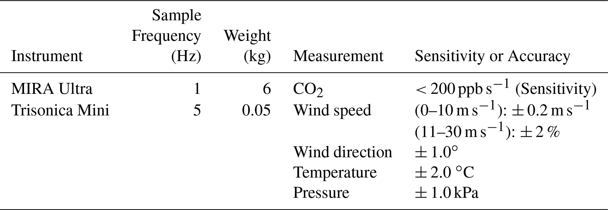
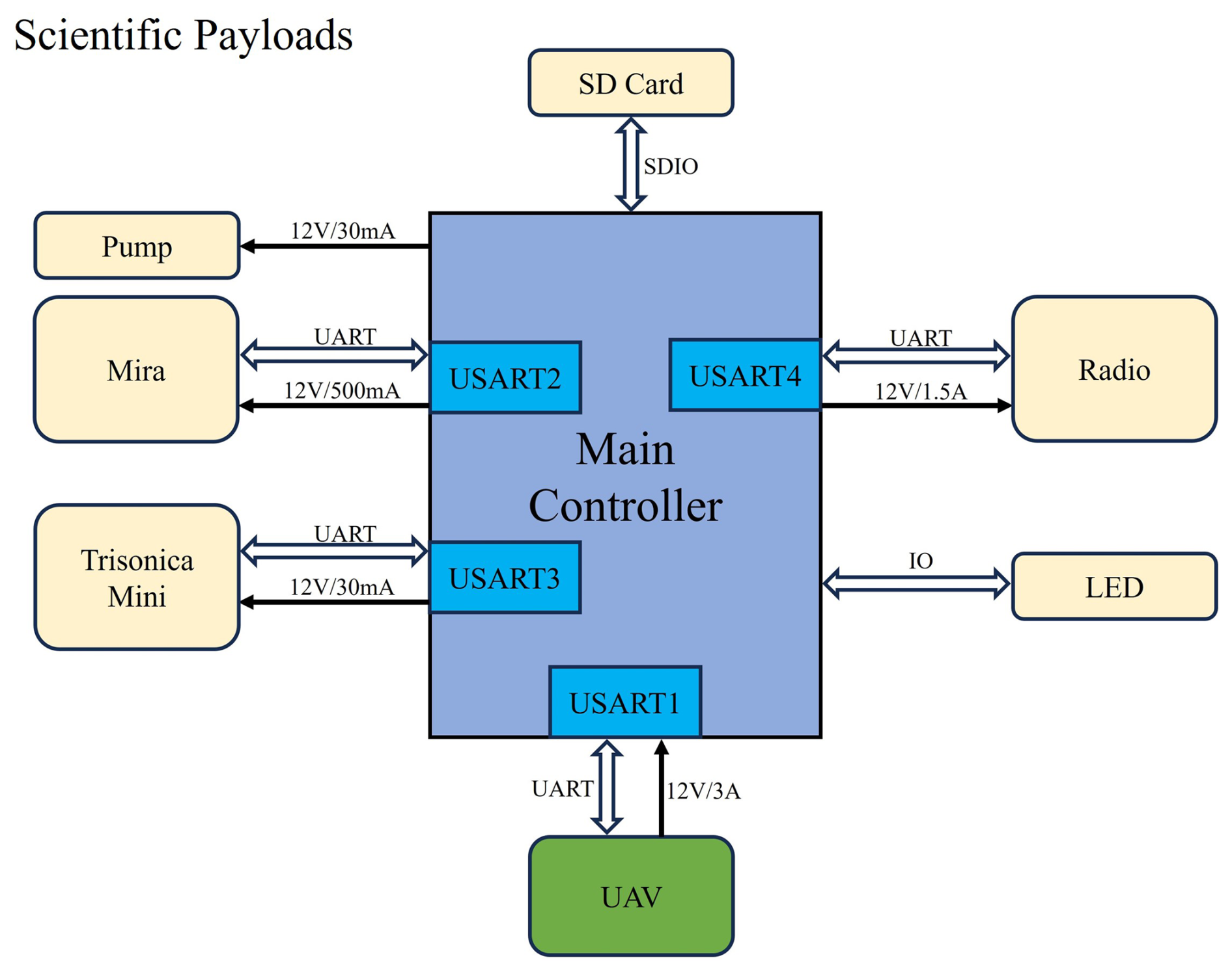
Figure 1 Diagram of the scientific payloads on the UAV-based flux measurement system. The light-emitting diode (LED) is used as a status indicator to display the operating state of the UAV measurement system during flight and ground testing.

2.2 Field site description

The UAV-based field measurements were conducted at the Qianyanzhou Experimental Station (26^∘44^′29^′′ N, 115^∘03^′29^′′ E) located in Jiangxi Province, southern China. This station is one of the core flux observation sites of the China Flux Observation Research Network (ChinaFLUX) and is equipped with a comprehensive EC measurement system (Yu et al., 2006). The flux tower has a height of approximately 43 m above ground, with the EC system installed at 31 m above ground level, while the mean forest canopy height is about 18 m.

The long-term observation site, 1 ha in size and centred on the flux tower, is dominated by plantation forests, primarily consisting of Pinus massoniana, Cunninghamia lanceolata, and Pinus elliottii arranged in a strip-mixed pattern with an approximate ratio of 49:48:3, respectively (Huang et al., 2007). The region experiences a typical subtropical monsoon climate, characterized by prevailing southerly winds in summer and northerly winds in winter. The mean annual air temperature is 17.9 °C, and the mean annual precipitation is approximately 1490 mm, with most rainfall occurring between March and June.

To evaluate the performance of the UAV platform for CO₂ vertical flux measurements, flights were conducted from a UAV take-off location approximately 160 m southeast of the flux tower, where the relatively open forest structure allowed safe UAV take-off and landing (Fig. 2a). The UAV-derived fluxes were then directly compared with tower-based measurements. The terrain within approximately 1 km² surrounding the flux tower is characterized by continuous low hills and gentle slopes, with slope angles of approximately 2.8–13.5° and local relative elevation differences of approximately 10–30 m. The approximately 15 m elevation difference between the flux tower and the UAV take-off location is therefore part of the naturally undulating low-hill terrain. Owing to this topographic variability, all UAV flight altitudes reported in this study are referenced to the take-off elevation of the UAV take-off location; consequently, the actual height above the local ground surface varied spatially along the flight path. Within a radius of approximately 350 m northwest of the UAV take-off location, only a limited number of low-rise buildings below the forest canopy used exclusively for scientific research are present, resulting in minimal anthropogenic influence on the measured CO₂ fluxes. Such an experimental condition provides a representative forest ecosystem setting in which UAV-derived fluxes can be evaluated against flux tower observations.

From May 2023 to December 2024, a total of 209 UAV flights were conducted at the site. After quality control, including the removal of records affected by rainfall and other conditions that could compromise instrument performance, 168 flights, corresponding to approximately 70 h of cumulative flight time, were retained for analysis. These included 40 flights in spring, 55 in summer, 53 in autumn, and 20 in winter, with seasons defined according to the Northern Hemisphere meteorological seasons: March–May, June–August, September–November, and December–February, respectively.

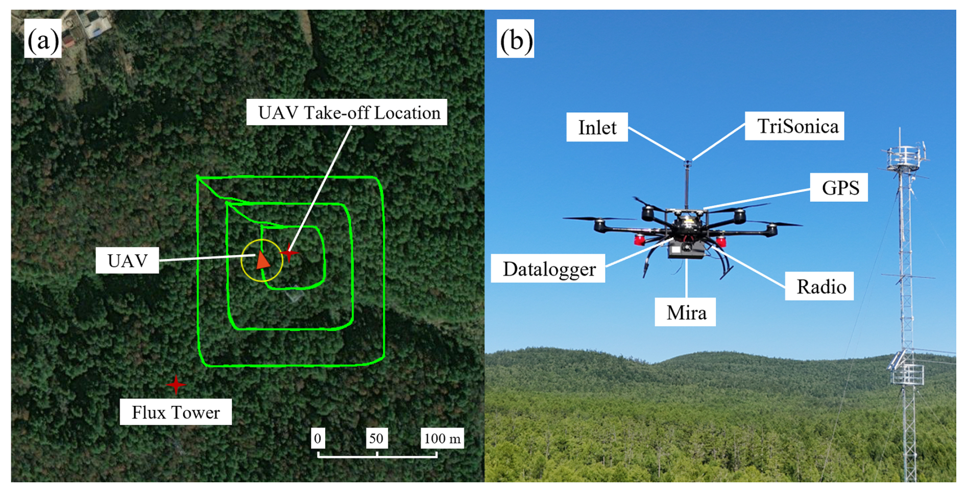
Figure 2 (a) A top-down view of the UAV's flight tracks from a representative flight. The green flight tracks represent the ‌box pattern‌, categorized into three box sizes: 50 × 50 × 50 m³, 100 × 100 × 50 m³, and 150 × 150 × 50 m³. The flux tower location, where EC measurements of vertical CO₂ fluxes are continuously conducted, and the UAV take-off location for the profile pattern are indicated in the figure. The straight-line distance between the flux tower and the UAV take-off location is approximately 160 m. All UAV flights were conducted following the same predefined flight routes. (b) The instrumented UAV platform; the flux tower can be seen in the background.

2.3 Flight patterns

Two complementary flight strategies were executed in this study: a box pattern and a profile pattern (Fig. 3a). The box pattern consists of a closed rectangular flight path flown above the forest canopy at multiple altitudes, enabling sampling of horizontal CO₂ transport across a defined control volume. Box flights were conducted at heights of 35, 40, 45, 50, 60, and 85 m above ground level. Using flight-path fitting and screen linear interpolation, the 3-D spatial distributions of the CO₂ mole fraction anomaly, wind vectors, and air density were reconstructed within the box domain. In the present study, we reconstructed the spatially distributed data for visualization purposes only (Fig. 3b), but computed the horizontal fluxes using the original observations directly. Flight-path fitting refers to the construction of a smooth, closed loop from the discrete UAV trajectories at all altitudes, thereby defining the four virtual vertical surfaces of the box. Screen linear interpolation refers to the mapping of CO₂ mole fractions and corrected wind speed measurements observed along the flight path onto a regular 2-D grid on the vertical surfaces for visualization of spatial patterns.

The profile pattern was designed to capture vertical gradients of CO₂ mole fractions, wind speed, and air density from near the surface to the top measurement height. Each box-pattern flight was paired with a vertical profile, and all measurements were completed within approximately 20 min to ensure consistency of the sampled air mass in the control volume. Vertical CO₂ fluxes were computed from the profile data using the gradient method (Sect. 3.2.2), with the analysis height range defined by the lowest and highest box levels (35–85 m). Because the EC system is installed at 31 m above ground level, UAV-derived CO₂ vertical fluxes were calculated using profile data collected at 26 and 36 m, thereby bracketing the EC measurement height for comparison with the tower-based EC measurements.

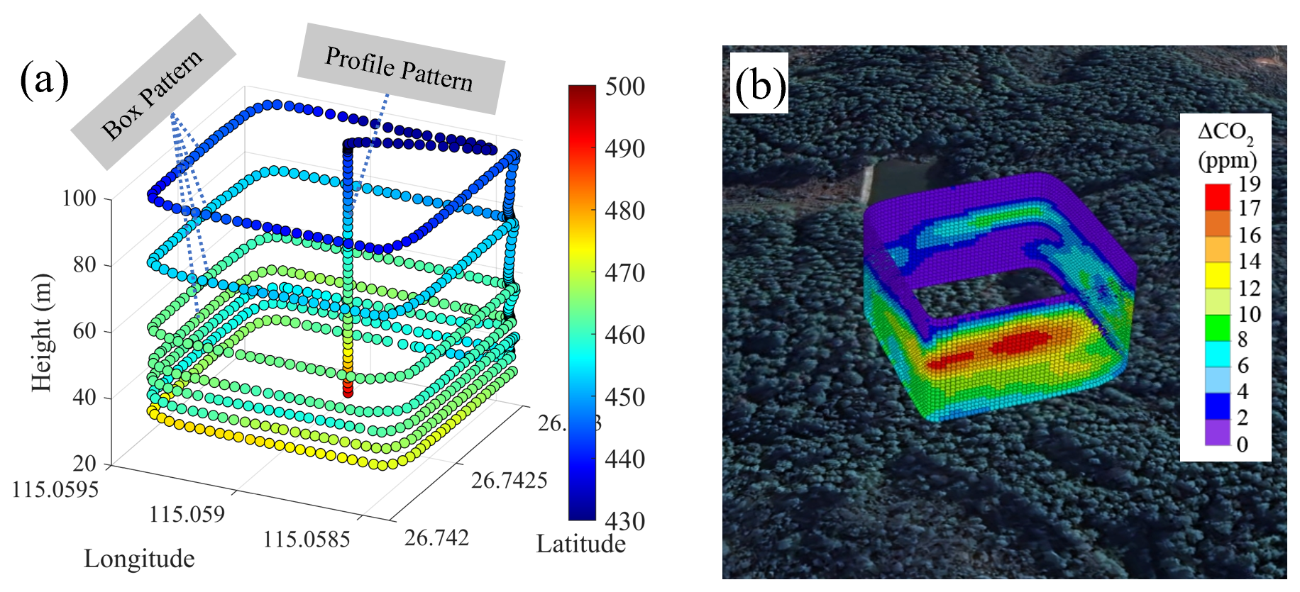
Figure 3 Overview of flight patterns.‌ (a) Two distinct flight strategies: box pattern and the profile pattern. (b) The spatial distribution of CO₂ mole fraction anomaly obtained through flight-path fitting and screen linear interpolation for the morning flight conducted from 07:00 to 07:30 UTC on 8 August 2024.

3 Methodologies

3.1 Wind speed calibration

To obtain accurate and reliable wind speed measurements, the raw data acquired by the ultrasonic anemometer were processed using a dedicated wind speed calibration algorithm. This algorithm, developed by Yang et al. (2025), was specifically developed for the UAV platform and the mounted instrumentation used in this study, and employs computational fluid dynamics (CFD) simulations to characterize the flow-field distortion by the UAV rotor-induced airflows. Hundreds of simulation scenarios were conducted, encompassing a wide range of flight altitudes, wind directions, and ambient wind speeds, in order to quantify the influence of rotor-induced airflow disturbances on wind measurements. The simulated disturbance fields were subsequently combined with UAV motion and attitude compensation schemes, yielding a comprehensive correction algorithm that simultaneously accounts for UAV translation, rotation, and rotor effects. The algorithm was validated with 3-D wind measurements at multiple levels on an 80 m meteorological tower (Yang et al., 2025). All wind measurements used in this study were corrected using this algorithm, ensuring consistency and comparability with reference-grade wind observations.

3.2 UAV-based estimation of the net CO₂ emission rate

CO₂ emissions associated within the control volume defined by the virtual box were quantified using a mass-balance framework that integrates measurements obtained from box-pattern and profile-pattern UAV flights. Throughout this study, the term “net CO₂ emission rate” refers to a signed, control-volume-integrated mass-balance quantity expressed in (kg h⁻¹). Positive values represent net CO₂ release from the control volume and may include CO₂ supplied by vegetation and soil respiration, whereas negative values represent net CO₂ uptake, primarily associated with vegetation photosynthesis. Thus, a negative net emission rate indicates that the forest acts as a net CO₂ sink during the measurement period. This approach assumes that CO₂ mole fraction and wind fields across the control volume boundaries are sampled with sufficient spatial coverage and that atmospheric conditions remain steady or quasi-steady during the measurement period. Under these conditions, the net emission rate can be inferred from the fluxes crossing the boundaries of the control volume.

According to the divergence theorem, the rate of change of mass of a stable compound within a control volume equals the surface integral of the mass flux through its enclosing surfaces. Consequently, the net CO₂ emission rate within the volume equals the net outward flux integrated across all box wall surfaces, where positive flux contributions represent CO₂ mass leaving the box and negative flux contributions represent CO₂ mass entering the box. Based on the integral form of the continuity equation, the emission rate within the control volume enclosed by the box pattern can be expressed as

$$\begin{array}{}\text{(1)}& E_{\mathrm{C}}=E_{\mathrm{C},\mathrm{H}}+E_{\mathrm{C},\mathrm{HT}}+E_{\mathrm{C},\mathrm{V}}+E_{\mathrm{C},\mathrm{VT}}-E_{\mathrm{C},\mathrm{M}}\end{array}$$

where E_C denotes the net CO₂ emission rate within the control volume, E_C,H and E_C,V denote the integrals of horizontal and vertical advective fluxes through the box walls, respectively; E_C,HT and E_C,VT represent the integrated turbulent fluxes in the horizontal and vertical directions, respectively, and E_C,M accounts for changes in CO₂ mass associated with air-density variations. Equation (1) forms the basis of the TERRA emission inversion model (Gordon et al., 2015).

To investigate the contributions of individual transport components to the net CO₂ emission, the TERRA framework was updated here, particularly with respect to the treatment of the vertical flux, so that the vertical turbulent flux could be calculated directly from the UAV measurements rather than parametrized through an entrainment assumption.

For clarity, u, v, and w denote the instantaneous east-west, north-south, and vertical wind-speed components, respectively, with positive values indicating eastward, northward, and upward flow. Throughout this section, c denotes the instantaneous CO₂ mass concentration (mg m⁻³), calculated as: c=M_Rχ_Cρ_air, where χ_C is the measured CO₂ mole fraction (ppm), ρ_air is the concurrently measured air density (kg m⁻³), and M_R is the ratio of the molar mass of CO₂ to that of air. With these units, the equation yields c directly in mg m⁻³. For the Reynolds decomposition of the concurrent 10 Hz tower observations, each variable $q\in \mathit{\{}u,v,w,c\mathit{\}}$ was decomposed over non-overlapping 30 min intervals as: $\stackrel{\mathrm{‾}}{q}=\frac{\mathrm{1}}{k}\sum _{i=\mathrm{1}}^k{q}_i$, and turbulent fluctuation: $q_i{}^{\prime }=q_i-\stackrel{\mathrm{‾}}{q}$, where k is the number of valid observations and is nominally 18 000 for a complete interval.

These concurrent tower observations were used to assess the relative importance of the mean and turbulent wind components and, consequently, the relative magnitudes of the corresponding transport terms in Eq. (1). Further details of the tower-data processing are provided in Sect. 3.4. For the horizontal component, the mean east-west wind component, $\left|\stackrel{\mathrm{‾}}{u}\right|$, was typically 2–3 m s⁻¹, whereas the 95th percentile of |u^′|, calculated from the instantaneous 10 Hz deviations from the corresponding 30 min means defined above, was less than 0.1 m s⁻¹. Thus, the mean horizontal wind component was more than one order of magnitude larger than the turbulent fluctuation, indicating that E_C,H was substantially larger than E_C,HT under the observed conditions.

For the vertical component, the opposite relationship was observed. The magnitude of the mean vertical wind component, $\left|\stackrel{\mathrm{‾}}{w}\right|$, was typically less than 0.02 m s⁻¹, whereas the 95th percentile of |w^′| reached approximately 0.3 m s⁻¹. Thus, the vertical turbulent fluctuation was more than one order of magnitude larger than the mean vertical wind component, indicating that E_C,VT was substantially larger than E_C,V. On this basis, the vertical advective term was neglected in Eq. (1).

The density-related term (E_C,M) can be expressed as

$$\begin{array}{}\text{(2)}& E_{\mathrm{C},\mathrm{M}}=\iiint c{\displaystyle \frac{\mathrm{d}{\mathit{\rho }}_{\mathrm{air}}}{\mathrm{d}t}}\mathrm{d}x\mathrm{d}y\mathrm{d}z\left(\mathrm{2}\right)\end{array}$$

where t is time, and x, y, and z denote the east-west, north-south, and vertical spatial coordinates, respectively. Thus, x and y describe the horizontal directions, whereas z represents the vertical direction.

Because the vertical extent (≈50 m), horizontal extent (≈150 m), and duration of the UAV flights are limited, air-density variation over time $\frac{\mathrm{d}{\mathit{\rho }}_{\mathrm{air}}}{\mathrm{d}t}$ within the control volume can be assumed to be negligible, and E_C,M was therefore neglected. Accurate estimation of the remaining flux terms (E_C,H and E_C,VT) enables computation of the net CO₂ emission rate. The reliability of the box-pattern approach for resolving CO₂ emission is further supported by Han et al. (2024), who conducted a series of controlled UAV-based CO₂ validation experiments over an industrial coking facility.

3.2.1 Computation of the horizontal advective contribution to the net CO₂ emission rate

The horizontal advective contribution to the net CO₂ emission rate was derived from box-pattern measurements by integrating the horizontal advective CO₂ flux across the four vertical walls of the virtual box. The integrated horizontal CO₂ emission rate can be written as

$$\begin{array}{}\text{(3)}& E_{\mathrm{C},\mathrm{H}}=∯c\left(s,z\right)U_{⟂}\left(s,z\right)\mathrm{d}s\mathrm{d}z\end{array}$$

where E_C,H is the horizontal advective contribution to the net CO₂ emission rate and $U_{⟂}(s,z)$ is the wind speed component normal to the flight path at point P(s,z). Here, the along-track coordinate s is defined along the horizontal flight trajectory, which formed a closed loop around the control volume. The start and end points of s therefore correspond to the same spatial location, ensuring a closed control volume boundary and avoiding gaps in the reconstructed flux field. Point P denotes the sampling location at along-track position s and flight altitude z.

For each altitude level z_i, the line flux F(z_i) was first calculated from the box-pattern data as

$$\begin{array}{}\text{(4)}& F\left(z_i\right)=\sum _{j=\mathrm{1}}^{N_i}c\left(s_j,z_i\right)\cdot U_{⟂}\left(s_j,z_i\right)\cdot \mathrm{\Delta }{s}_j\end{array}$$

where j denotes the sampling point index along the flight path at altitude z_i, N_i is the total number of sampling points at altitude z_i, and Δs_j represents the along-track distance between two consecutive sampling points along the closed-loop flight trajectory.

For each UAV flight, one closed-loop transect was conducted at each measurement height, yielding one line-flux value for that height. To obtain fluxes for discrete altitude intervals, line-flux values at adjacent measurement heights were averaged in the vertical direction. The resulting layer-averaged fluxes were then used in the horizontal advective contribution to the net CO₂ emission rate calculation

$$\begin{array}{}\text{(5)}& \begin{array}{rl}{E}_{\mathrm{C},\mathrm{H}}& =\sum _{i=\mathrm{1}}^{n}F\left(z_i\right)\mathrm{\Delta }{z}_i=\sum _{i=\mathrm{1}}^n\\ & \left(\sum _{j=\mathrm{1}}^{N_i}c(s_j,z_i)U_{⟂}(s_j,z_i)\mathrm{\Delta }{s}_j\right)\mathrm{\Delta }{z}_i\end{array}\end{array}$$

where i denotes the vertical layer index from the first layer to the nth layer, n is the total number of vertical layers, and Δz_i is the thickness of the ith altitude interval. In this study, the first observed altitude layer z₁ corresponds to the lowest UAV sampling height (35 m above ground level).

3.2.2 Computation of the vertical turbulent contribution to the net CO₂ emission rate

The vertical turbulent contribution to the net CO₂ emission rate was estimated from profile measurements using the gradient method, which relates turbulent scalar fluxes to vertical gradients of the scalar quantity. In practice, vertical profiling over forested terrain is operationally challenging, and UAV measurements were conducted at a single representative location. The resulting vertical fluxes were compared with EC flux tower measurements to evaluate the reliability of the UAV-derived vertical flux estimates (see Sect. 4.2.1). This comparison was not intended to imply that vertical fluxes alone represent the full CO₂ mass balance of the control volume. Instead, the horizontal flux terms were calculated separately to quantify lateral CO₂ transport across the control volume boundaries, which provides information on local advection and spatial heterogeneity that cannot be obtained from vertical flux measurements alone.

Before calculating the vertical gradients, the UAV profiles of CO₂ mass concentration, horizontal wind-speed magnitude, and air temperature were smoothed using a seven-point moving average applied along the vertical profile. To distinguish these locally smoothed profile quantities from the 30 min temporal means used for the fixed EC tower data, a tilde is used throughout this subsection. Thus, $\stackrel{\mathrm{̃}}{c}\left(z\right)$, $\stackrel{\mathrm{̃}}{S}\left(z\right)$, and $\stackrel{\mathrm{̃}}{T}\left(z\right)$ denote the smoothed CO₂ mass concentration, horizontal wind-speed magnitude, and air temperature, respectively.

The vertical turbulent contribution to the net CO₂ emission rate was obtained by integrating the vertical CO₂ flux over the horizontal area enclosed by the box pattern. Assuming that the profile-derived vertical flux is representative of this area,

$$\begin{array}{}\text{(6)}& E_{\mathrm{C},\mathrm{VT}}=\iint F_{\mathrm{v}}\mathrm{d}x\mathrm{d}y=A\cdot F_{\mathrm{v}}\end{array}$$

where F_v denotes the CO₂ vertical flux and A is the horizontal area of the control volume.

According to the flux-gradient relationship (Kaimal and Finnigan, 1994), the vertical turbulent scalar flux is related to the vertical gradient of the smoothed scalar profile by

$$\begin{array}{}\text{(7)}& F_{\mathrm{v}}=-K_{\mathrm{C}}{\displaystyle \frac{\partial \stackrel{\mathrm{̃}}{c}}{\partial z}}\end{array}$$

where K_C is the turbulent exchange coefficient for CO₂.

A mixing-length formulation is used to estimate the turbulent exchange coefficient. The momentum eddy diffusivity is written as (Lee and Mahrt, 2005)

$$\begin{array}{}\text{(8)}& K_{\mathrm{M}}=l{u}_{*}\end{array}$$

where l is the mixing length, K_M is the exchange coefficient for momentum, and u_* is the friction velocity. Under neutral stratification conditions, the neutral mixing length above a displaced canopy is

$$\begin{array}{}\text{(9)}& l_{\mathrm{0}}=\mathit{\kappa }(z-d)\end{array}$$

where κ=0.4 is the von Kármán constant and d is the zero-plane displacement height.

To account for atmospheric stratification, a stability factor m is applied to the mixing length (Budyko et al., 1962),

$$\begin{array}{}\text{(10)}& l=m{l}_{\mathrm{0}}=m\mathit{\kappa }(z-d)\end{array}$$

where m is the stratification correction parameter, determined as a function of the gradient Richardson number (‌R_i) according to Budyko et al. (1962):

$$\begin{array}{}\text{(11)}& m=(\mathrm{1}-R_i{)}^{\mathrm{1}/\mathrm{2}}\end{array}$$

where R_i is the gradient Richardson number. For the finite vertical separation used in the UAV profile calculation, R_i is approximated by the bulk Richardson number R_B

$$\begin{array}{}\text{(12)}& \begin{array}{rl}{R}_i& \approx R_{\mathrm{B}}={\displaystyle \frac{g}{{\stackrel{\mathrm{̃}}{T}}_{\mathrm{m}}}}\cdot {\displaystyle \frac{({\stackrel{\mathrm{̃}}{T}}_{\mathrm{2}}-{\stackrel{\mathrm{̃}}{T}}_{\mathrm{1}})(z_{\mathrm{2}}-z_{\mathrm{1}})}{({\stackrel{\mathrm{̃}}{S}}_{\mathrm{2}}-{\stackrel{\mathrm{̃}}{S}}_{\mathrm{1}}{)}^{\mathrm{2}}}},\\ {\stackrel{\mathrm{̃}}{T}}_{\mathrm{m}}& =({\stackrel{\mathrm{̃}}{T}}_{\mathrm{1}}+{\stackrel{\mathrm{̃}}{T}}_{\mathrm{2}})/\mathrm{2}\end{array}\end{array}$$

where g is gravitational acceleration; and the subscripts 1 and 2 denote values evaluated from the smoothed vertical profiles at the lower and upper heights z₁ and z₂, respectively. When applying the gradient method to estimate the flux, the vertical separation, $\mathrm{\Delta }z=z_{\mathrm{2}}-z_{\mathrm{1}}$, is typically chosen within a range of 1–10 m (Meredith et al., 2014). In this study, z₁ and z₂ are located 5 m below and 5 m above the target height, respectively, giving $\mathrm{\Delta }z=z_{\mathrm{2}}-z_{\mathrm{1}}=\mathrm{10}$ m.

Because the forest canopy is aerodynamically rough, the wind profile is expressed using the displacement-height form of the neutral logarithmic wind profile (Raupach, 1994). The smoothed horizontal wind-speed magnitude is written as

$$\begin{array}{}\text{(13)}& \stackrel{\mathrm{̃}}{S}\left(z\right)={\displaystyle \frac{u_{*}}{\mathit{\kappa }}}\ln {\displaystyle \frac{z-d}{z_{\mathrm{0}}}}\end{array}$$

where z₀ is the aerodynamic roughness length. Evaluating Eq. (13) at z₁ and z₂ and eliminating z₀ gives the friction velocity as

$$\begin{array}{}\text{(14)}& u_{*}=\mathit{\kappa }{\displaystyle \frac{{\stackrel{\mathrm{̃}}{S}}_{\mathrm{2}}-{\stackrel{\mathrm{̃}}{S}}_{\mathrm{1}}}{\ln \left[\right(z_{\mathrm{2}}-d)/(z_{\mathrm{1}}-d\left)\right]}}\end{array}$$

Assuming K_C = K_M for the scalar-transfer calculation used here, substituting Eqs. (10), (11), and (14) into Eq. (8) gives

$$\begin{array}{}\text{(15)}& K_{\mathrm{C}}={\mathit{\kappa }}^{\mathrm{2}}(\mathrm{1}-R_i{)}^{\mathrm{1}/\mathrm{2}}{\displaystyle \frac{{\stackrel{\mathrm{̃}}{S}}_{\mathrm{2}}-{\stackrel{\mathrm{̃}}{S}}_{\mathrm{1}}}{\ln \left[\right(z_{\mathrm{2}}-d)/(z_{\mathrm{1}}-d\left)\right]}}(z-d)\end{array}$$

Using the finite-layer formulation employed in the gradient calculation, the wind-speed and CO₂ differences between z₁ and z₂ are expressed over the same logarithmic height interval. Substitution into Eq. (7) gives

$$\begin{array}{}\text{(16)}& F_{\mathrm{v}}={\mathit{\kappa }}^{\mathrm{2}}(\mathrm{1}-R_i{)}^{\mathrm{1}/\mathrm{2}}{\displaystyle \frac{\left({\stackrel{\mathrm{̃}}{S}}_{\mathrm{2}}-{\stackrel{\mathrm{̃}}{S}}_{\mathrm{1}}\right)({\stackrel{\mathrm{̃}}{c}}_{\mathrm{1}}-{\stackrel{\mathrm{̃}}{c}}_{\mathrm{2}})}{{\left\{\ln \left[\right(z_{\mathrm{2}}-d)/(z_{\mathrm{1}}-d\left)\right]\right\}}^{\mathrm{2}}}}\end{array}$$

The corresponding vertical turbulent contribution is

$$\begin{array}{}\text{(17)}& E_{\mathrm{C},\mathrm{VT}}=A{\mathit{\kappa }}^{\mathrm{2}}(\mathrm{1}-R_i{)}^{\mathrm{1}/\mathrm{2}}{\displaystyle \frac{\left({\stackrel{\mathrm{̃}}{S}}_{\mathrm{2}}-{\stackrel{\mathrm{̃}}{S}}_{\mathrm{1}}\right)({\stackrel{\mathrm{̃}}{c}}_{\mathrm{1}}-{\stackrel{\mathrm{̃}}{c}}_{\mathrm{2}})}{{\left\{\ln \left[\right(z_{\mathrm{2}}-d)/(z_{\mathrm{1}}-d\left)\right]\right\}}^{\mathrm{2}}}}\end{array}$$

For each UAV flight, F_v and the corresponding vertical turbulent contribution E_C,VT were calculated from the paired vertical profile measurements rather than from the box-pattern observations. For the comparison with the EC system, z₁=26 m and z₂=36 m above the UAV take-off elevation are used, and the resulting flux is assigned to the midpoint height of approximately 31 m. The reliability of the vertical flux estimates from Eq. (16) is evaluated against the EC flux tower observations in Sect. 4.2.1.

3.3 Computation of uncertainties

The uncertainty of the UAV-derived CO₂ emission estimates was evaluated by considering both measurement-related uncertainties and methodological uncertainties associated with the UAV-based 3-D flux quantification framework. The net CO₂ emission, E_C, was calculated from the horizontal transport contribution, E_C,H, and the vertical turbulent contribution, E_C,VT. Therefore, uncertainty was assessed for the input variables and calculation procedures involved in both terms.

The measurement-related uncertainty was divided into two components: CO₂ analyzer uncertainty (${\mathit{\delta }}_{{\mathrm{CO}}_{\mathrm{2}}}$) and wind measurement uncertainty (δ_V). Assuming that the two uncertainty components are independent and represent standard-deviation-type uncertainties, they were combined in quadrature to obtain the measurement-propagated uncertainty:

$$\begin{array}{}\text{(18)}& {\mathit{\delta }}_{\mathrm{meas}}^{\mathrm{2}}={\mathit{\delta }}_{{\mathrm{CO}}_{\mathrm{2}}}^{\mathrm{2}}+{\mathit{\delta }}_{\mathrm{V}}^{\mathrm{2}}\end{array}$$

Here, ${\mathit{\delta }}_{{\mathrm{CO}}_{\mathrm{2}}}$ represents the uncertainty associated with the measured CO₂ mole fraction, including analyzer precision, calibration uncertainty, and short-term measurement noise. Wind-related uncertainty was included in δ_V, which includes uncertainty arising from the ultrasonic anemometer measurements, and the wind-correction procedure used to correct for these effects.

3.3.1 CO₂ analyzer uncertainty

The CO₂ analyzer uncertainty was estimated from the performance of the MIRA CO₂ analyzer and the ground-based intercomparison with the LI-7500 analyzer. The MIRA analyzer has an accuracy better than 0.2 ppm, whereas the CO₂ variations resolved during UAV sampling frequently exceeded several to tens of ppm. Therefore, the relative uncertainty associated with the CO₂ mole fraction measurement was small compared with the observed CO₂ gradients used in the flux calculations. In addition, the analyses shown in Figs. 4 and 5 indicate that the error caused by the MIRA CO₂ analyzer is almost negligible. Therefore, the contribution of ${\mathit{\delta }}_{{\mathrm{CO}}_{\mathrm{2}}}$ was conservatively set to 1 %.

3.3.2 Wind measurement uncertainty

Wind measurement uncertainty was treated as a separate uncertainty component because wind speed and wind direction directly affect the horizontal transport term, and the turbulent exchange parameters used in the vertical flux calculation. For the uncertainty introduced by the wind-speed correction, based on the validation experiment reported by Yang et al. (2025), the corrected UAV wind speed showed a root mean square relative error of 0.28 compared with the meteorological tower reference measurements. Therefore, a conservative relative uncertainty of 28 % was assigned to the residual wind-correction uncertainty. Additionally, the ultrasonic anemometer used on the UAV has a wind speed accuracy of ±0.2 m s⁻¹ and a wind direction accuracy of ±1°. For typical flight-level wind speeds of 4–6 m s⁻¹, this corresponds to a relative error of about 5 % in the horizontal wind components. Assuming that the residual wind-correction uncertainty and the instrument-related uncertainty were independent relative standard uncertainties, they were combined in quadrature and the final contribution of δ_V was estimated to be 28.5 %.

3.3.3 Methodological uncertainty

In addition to measurement-related uncertainty, the UAV-based flux estimates are also affected by methodological uncertainty associated with the flux quantification framework itself.

For the horizontal transport term, E_C,H, methodological uncertainty arises mainly from discrete sampling along the box-pattern flight path and the spatial reconstruction of lateral boundary fluxes. The resulting uncertainty is collectively referred to as δ_spatial. Because the UAV samples the control volume boundaries along discrete trajectories rather than continuously measuring the entire boundary surface, the reconstructed lateral flux depends on the interpolation or averaging method used to integrate the boundary observations. To evaluate spatial reconstruction uncertainty (δ_spatial), E_C,H was recalculated using three treatments of the discrete box-pattern observations, including linear interpolation, nearest-neighbor interpolation, and segment averaging. Linear interpolation is the method used for the primary E_C,H calculation in this study and was therefore treated as the reference method. The E_C,H estimates obtained using nearest-neighbor interpolation and segment averaging were compared with those obtained using linear interpolation, and the resulting relative differences were used to quantify the sensitivity of to the spatial-reconstruction method. Because the purpose of this analysis was to assess the methodological sensitivity of the flux calculation rather than to derive a separate methodological uncertainty for every individual UAV flight, three representative cases spanning different seasons and observational conditions were selected for the analysis: spring morning (12 May 2024), summer noon (20 August 2023), and autumn noon (3 December 2024). Applying the full set of alternative reconstruction and recalculation procedures to all UAV flights would require substantial additional computation. Given that the uncertainty analysis in the present study already considers the major measurement-related and methodological uncertainty sources, these representative cases were used to provide a practical assessment of the sensitivity associated with spatial reconstruction. Relative to the linear-interpolation results, the nearest-neighbor and segment-averaging methods produced differences of 6 % and 8 %, respectively. To provide a conservative estimate, the larger value was adopted, and δ_spatial=8 % was therefore used to represent the methodological uncertainty associated with spatial reconstruction of the lateral boundary fluxes.

For the vertical turbulent contribution term, E_C,VT, the methodological uncertainty was mainly associated with the flux-gradient approach and, in particular, with the estimation of the turbulent exchange coefficient from wind-related variables, including the 3-D wind components and friction velocity. To evaluate the sensitivity of E_C,VT to this part of the methodology, perturbations in the wind-related inputs were propagated through the flux-gradient calculation (δ_gradient). Based on the wind-correction validation described above, a relative perturbation of 28.5 % was applied to the wind-related inputs used to derive the turbulent exchange coefficient. The same three representative cases used for the uncertainty analysis of E_C,H were also used for E_C,VT. The resulting uncertainties were 3 %, 2 %, and 5 % for the three representative cases. The largest value (5 %) was used to characterize the sensitivity of the vertical flux-gradient calculation to wind-related perturbations. Because the sensitivity of the vertical flux-gradient calculation was derived by propagating the wind-related uncertainty, δ_gradient and δ_V were not treated as independent uncertainty components. To avoid double counting, δ_gradient was therefore excluded from the quadrature calculation of the total uncertainty. Assuming that the remaining uncertainty components are independent, the total relative uncertainty (δ_combined) was calculated:

$$\begin{array}{}\text{(19)}& {\mathit{\delta }}_{\mathrm{combined}}^{\mathrm{2}}={\mathit{\delta }}_{{\mathrm{CO}}_{\mathrm{2}}}^{\mathrm{2}}+{\mathit{\delta }}_{\mathrm{V}}^{\mathrm{2}}+{\mathit{\delta }}_{\mathrm{spatial}}^{\mathrm{2}}\end{array}$$

3.3.4 Total estimated uncertainties

By combining the uncertainy components, including CO₂ analyzer uncertainty (${\mathit{\delta }}_{{\mathrm{CO}}_{\mathrm{2}}}$), wind measurement uncertainty (δ_V), and methodological uncertainty (δ_spatial), the total relative uncertainty of the UAV-derived CO₂ emission rates can be obtained through quadrature addition. This yields a total relative uncertainty of approximately 29.6 %, which is rounded to approximately 30 %.

3.4 Stationary tower-based data processing

The EC system installed at the flux tower consists of a 3-D ultrasonic anemometer (CSAT3, Campbell Scientific, USA), an open-path ${\mathrm{CO}}_{\mathrm{2}}/{\mathrm{H}}_{\mathrm{2}}\mathrm{O}$ analyzer (LI-7500, LI-COR Biosciences, USA), and a datalogger (CR3000, Campbell Scientific, USA). Raw data are acquired at a sampling frequency of 10 Hz. In the present study, concurrent EC data from the flux tower were processed after correcting the time lag between wind and gas measurements following Sahlée et al. (2007), and standard quality-control procedures were applied to the turbulence data (Sect. S1 in the Supplement).

Fluxes were computed over 30 min averaging intervals, and coordinate rotation, virtual temperature correction, and frequency-response correction were applied to ensure high-quality vertical flux estimates. For the EC calculations, the measured wind components were first transformed into a streamline coordinate system through coordinate rotation. In this rotated coordinate system, u_s denotes the streamwise wind component aligned with the mean horizontal wind direction. Following standard EC formulations (Webb et al., 1980; Baldocchi, 2003), the friction velocity (u_*) and scalar fluxes (F_v) were computed as

$$\begin{array}{}\text{(20)}& {\displaystyle }& {\displaystyle }{u}_{*}=(-\stackrel{\mathrm{‾}}{u_{\mathrm{s}}^{\prime }w{}^{\prime }}{)}^{\mathrm{1}/\mathrm{2}}\text{(21)}& {\displaystyle }& {\displaystyle }{F}_{\mathrm{v}}=\stackrel{\mathrm{‾}}{w{}^{\prime }c{}^{\prime }}\end{array}$$

where the primes denote the turbulent fluctuations defined in Sect. 3.2, which were calculated relative to the corresponding non-overlapping 30 min means.

4 Results and discussion

4.1 Gas analyzer comparison test

To evaluate the consistency between the two CO₂ analyzers, a ground-based co-located intercomparison experiment was conducted using the open-path ${\mathrm{CO}}_{\mathrm{2}}/{\mathrm{H}}_{\mathrm{2}}\mathrm{O}$ gas analyzer (LI-7500) employed in the EC system and the closed-path analyzer (MIRA) used on the UAV. During the experiment, the two analyzers were placed side by side at the same ground location. Their sampling inlets were positioned at the same height and as close to each other as practicable to ensure that both instruments sampled the same air mass simultaneously. The experiment was conducted from 21:00 to 22:00 LT on 12 August 2024 (Fig. 4), with the LI-7500 operating at 10 Hz and the MIRA analyzer at 1 Hz. A fixed time lag of 5 s, associated with air flow through the sampling line, was applied to synchronize the MIRA measurements with the LI-7500 data.

Figure 4 Comparison of CO₂ mole fractions measured by the LI-7500 and MIRA analyzers.

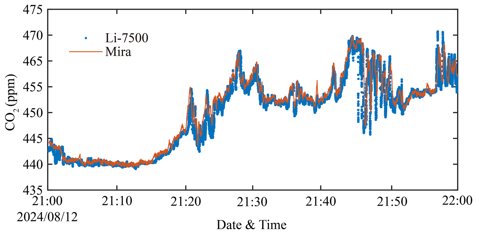
As shown in Fig. 4, the CO₂ mole fractions measured by the two instruments exhibit highly consistent temporal variability, although small differences in absolute values and short-term fluctuations are present. Both datasets show a pronounced increase in CO₂ mole fraction during the initial phase of the experiment, followed by enhanced variability with multiple peaks, and sustained elevated mole fractions during the later period. The overall temporal coherence between the two datasets is strong, indicating that both instruments capture the same underlying CO₂ fluctuation dynamics. The MIRA measurements, with an average value of approximately 451.7 ppm, tended to report slightly lower CO₂ mole fractions than the LI-7500 measurements, which had an average value of approximately 451.8 ppm. This attenuation is primarily attributed to high-frequency losses associated with the closed-path sampling system, including viscous damping and signal smoothing during sample transport through the $\mathrm{1}/\mathrm{8}$ in. outer-diameter polytetrafluoroethylene (PTFE) sampling tube. Because the sampling tube used in this study was relatively short (approximately 0.5 m) and the sample residence time inside the tube was 0.5 s, its influence on CO₂ measurements is expected to be limited. Such attenuation is a well-documented characteristic of closed-path systems and does not compromise the ability of the analyzer to resolve mean CO₂ mole fraction levels and mesoscale variability (Burba et al., 2012; Metzger et al., 2016). In summary, despite minor attenuations at high frequencies, the closed-path MIRA analyzer demonstrates strong agreement with the EC-based LI-7500 measurements, supporting its suitability for CO₂ measurements from the UAV-based platform.

Further, the scatterplot of the CO₂ measurement results from both instruments, shown in Fig. 5, reveals a strong linear relationship. The data are closely distributed around a narrow band of the fitted linear regression line, with a Pearson correlation coefficient of r=0.986. Because both analyzers are subject to measurement uncertainties, reduced major axis (RMA) regression was applied. The RMA regression yielded a slope of 0.966 and an intercept of 1.64 ppm. The close clustering of the data points around the fitted line indicates low random error and high precision between the two instruments. This regression result indicates that the UAV observations were able to capture temporal variability in CO₂ in the real atmosphere, such as minute-scale increases, decreases, and multi-peak structures. In addition, the calculations of the horizontal line flux divergence and the vertical flux both require subtraction of the background CO₂ mole fraction and estimation of the CO₂ gradient, respectively. Therefore, the systematic bias between the two instruments is expected to have a negligible impact on the flux calculations.

Figure 5 Scatterplot comparison of CO₂ mole fractions measured by the UAV-mounted MIRA analyzer and the flux-tower LI-7500 analyzer. The orange line denotes the RMA regression. The regression yielded a slope of 0.966 and an intercept of 1.64 ppm, with r=0.986, indicating strong agreement between the two instruments under field conditions.

4.2 In-flight comparison test

4.2.1 Seasonal variability of vertical fluxes

A key part of the present study is to determine reliable vertical flux measurements using the UAV platform over a forest ecosystem in complex terrains. To quantitatively evaluate the agreement between UAV-based profile retrievals and flux tower measurements, the UAV-derived vertical CO₂ flux (F_v) and friction velocity (u_*) are compared against their EC counterparts (Fig. 6). Because both datasets contain measurement uncertainties, the RMA regression (Smith, 2009; Warton et al., 2006) was used, which is more appropriate than ordinary least squares when neither dataset can be treated as error-free. The season-specific RMA slope, intercept, and r values are summarized in Table 3. For the comparison with the EC system installed at 31 m above ground, the UAV-derived vertical flux was calculated from the smoothed vertical profile measurements between z₁=26 and z₂=36 m relative to the UAV take-off elevation.

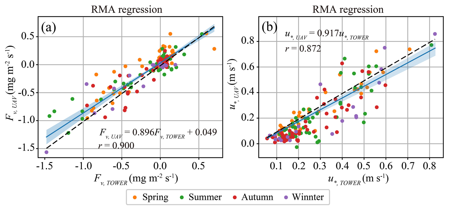
Figure 6 RMA regressions comparing UAV-based measurements with flux tower observations across all seasons. Panel (a) shows CO₂ flux (F_v) and panel (b) shows friction velocity (u_*). In both panels, the x axis represents the flux tower measurements and the y axis represents the UAV-based measurements. Points are colored by season (Spring, Summer, Autumn, Winter). The solid blue line denotes the RMA fit, the shaded band indicates the 95 % confidence interval (CI) of the regression line, and the dashed black line represents the 1:1 reference. The regression equations are expressed using the corresponding physical variables in each panel, and the Pearson correlation coefficient (r) is also reported.

Table 3 Seasonal RMA regression results comparing UAV-derived measurements with flux tower observations for CO₂ flux (F_v) and friction velocity (u_*). Seasons are defined according to the three-month meteorological seasons: spring (March–May), summer (June–August), autumn (September–November), and winter (December–February). For each season, the table reports the sample size (n), correlation coefficient (r), RMA slope and its 95 % confidence interval (CI), and the intercept. The u_* regressions are constrained to pass through the origin (intercept fixed at 0).

As shown in Fig. 6a, UAV-derived F_v,UAV exhibits a clear linear relationship with EC F_v,TOWER, with points generally distributed around the 1:1 line, indicating that the UAV approach captures the temporal variability of canopy-scale vertical CO₂ exchange. Table 3 further demonstrates consistently strong correlation coefficients across seasons (r=0.863–0.938). The slope, slightly lower than unity, suggests a modest “range compression” in the UAV-derived fluxes, meaning that the magnitudes tend to be slightly attenuated under strong emission or strong uptake conditions (large positive/negative fluxes). In spring, the slope is 0.928 (95 % CI: [0.777, 1.074], r=0.890), and in autumn the slope is 0.997 (95 % CI: [0.771, 1.281], r=0.863); both are close to unity and their confidence intervals encompass 1, suggesting good consistency in flux magnitude. In summer, the slope decreases to 0.801 (95 % CI: [0.694, 0.929], r=0.938), and the confidence interval does not include 1, indicating a smaller flux magnitude during periods of stronger exchange. Hence, the slightly lower-than-unity slope likely reflects enhanced nonstationarity and rapid scalar fluctuations during the peak growing season, which increase sensitivity to sampling height from ground and platform-related perturbations. In winter, the slope is 0.940 (95 % CI: [0.551, 1.079], r=0.917), showing strong correlation but larger uncertainty due to the smaller sample size (n=20).

Figure 6b shows a clear linear relationship between friction velocity $u_{*,\mathrm{UAV}}$ and $u_{*,\mathrm{TOWER}}$. Because u_* should physically approach zero under very weak turbulence, an origin-constrained regression (intercept fixed at 0) was used to avoid non-physical extrapolation from a free intercept. The full-sample RMA regression is:

$$\begin{array}{}\text{(22)}& u_{*,\mathrm{UAV}}=\mathrm{0.917}(\pm \mathrm{0.063})u_{*,\mathrm{TOWER}},r=\mathrm{0.872}\end{array}$$

This result indicates that the UAV platform captures the variations in turbulent intensity well (r=0.872), while the slope below unity suggests a slight multiplicative underestimation of u_* relative to tower observations. Regressions for different seasons (Table 3) further indicate that the best agreement occurs in spring, with a slope of 1.012 (95 % CI: [0.926, 1.093], r=0.942). In contrast, $u_{*,\mathrm{UAV}}$ shows a slight underestimation relative to $u_{*,\mathrm{TOWER}}$, with slopes of 0.915, 0.819, and 0.914 in summer, autumn, and winter, respectively. Taken together, Fig. 6 and Table 3 demonstrate that the fluxes and turbulence metrics derived from the UAV measurements reproduce well the tower-observed variability of both canopy-scale CO₂ exchange and key turbulence characteristics across all seasons (r=0.9 for F_v and r=0.872 for u_*), supporting the feasibility and robustness of such UAV profile measurements for monitoring above-canopy exchange. Nevertheless, two systematic features warrant attention: (i) F_v magnitudes tend to be slightly underestimated in summer (slope significantly <1), and (ii) u_* shows a slight overall underestimation under the origin-constrained regression.

4.2.2 Diurnal variability of vertical fluxes

To further evaluate the applicability and consistency of the UAV-based profiling method under different diurnal conditions, the UAV-derived F_v estimates were grouped and compared with results from EC observations in three time periods: early morning (06:00–08:00 local standard time, LST), noon (13:00–15:00 LST), and evening (19:00–21:00 LST). RMA regression was applied to both the vertical CO₂ flux (F_v) and the friction velocity (u_*) for each time period (Fig. 7), with the corresponding statistical results summarized in Table 4.

Figure 7 RMA regressions comparing UAV-based measurements with flux tower observations for (a) CO₂ flux (F_v) and (b) friction velocity (u_*) grouped by time of day. In both panels, the x axis represents the flux tower measurements and the y axis represents the UAV-based measurements. Data are separated into morning (06:00–08:00 LST), noon (13:00–15:00 LST), and evening (19:00–21:00 LST) and shown with different colors. Solid colored lines represent the RMA fits for each time period, and the shaded bands indicate the 95 % confidence intervals. The dashed black line denotes the 1:1 reference. Reported in each panel are the RMA slopes and their 95 % confidence intervals; the u_* regressions in panel (b) are constrained to pass through the origin (intercept fixed at 0).

As shown in Table 4, the RMA regressions for F_v exhibit relatively strong correlations during the early morning and midday periods (r=0.898, n=63 and r=0.867, n=55, respectively). The corresponding slopes are 0.871 (95 % CI: [0.732, 0.986]) for early morning and 0.916 (95 % CI: [0.750, 1.087]) for midday, both close to unity but slightly lower than 1, indicating a modest compression of the UAV-derived flux range relative to the EC measurements. Thus, although the UAV-based method reproduces the observed variability reasonably well, the magnitude of stronger fluxes tends to be attenuated. A possible explanation is that the gradient method derives fluxes from a smoothed CO₂ vertical profile over a finite height interval, which may partially attenuate steep or rapidly varying gradients under strong exchange conditions. Differences in temporal sampling between the relatively short UAV profile and the 30 min EC averaging interval may also contribute to the observed differences. This behavior is consistent with the seasonal-scale results presented in Sect. 4.2.1 and likely reflects the increased sensitivity of the gradient method to strong flux events under limited vertical sampling resolution and short-term nonstationary conditions.

Table 4 RMA regression statistics for comparisons between UAV-based measurements and flux tower observations, grouped by time of day (morning, noon, and evening). Results are reported for CO₂ flux (F_v) and friction velocity (u_*), including sample size (n), correlation coefficient (r), RMA slope, the 95 % confidence interval (CI) of the slope, and the intercept. For u_*, the regression is constrained to pass through the origin (intercept fixed at 0).

In contrast, the agreement for F_v deteriorates substantially during the evening period, with a low correlation coefficient (r=0.235, n=50) and a highly uncertain slope (1.730, with a 95 % confidence interval spanning both positive and negative values). The possible reason for such a comparison result is that, under low evening turbulence, both the UAV-based and EC-based flux measurements become less reliable, because the vertical turbulent exchange weakens and the relative influence of non-turbulent transport terms increases. Under such conditions, the UAV methodology is subject to larger uncertainties in the derived vertical fluxes and shows an apparent low bias relative to the EC measurements. It should be noted, however, that EC vertical flux measurements under such low turbulence conditions also bear large uncertainties, and hence this comparison only implies a low bias in the UAV methodology relative to the EC methodology, and does not indicate the absolute errors in the UAV-determined F_v nor that from the EC methodology. The diurnal variation of friction velocity (u_*) derived from the tower system (Fig. S1, Sect. S2 in the Supplement) shows a clear asymmetry between morning and evening transitions, with turbulence developing gradually after sunrise but decaying rapidly in the evening, which helps explain the poorer agreement under evening conditions. Furthermore, an analysis of the evening flux differences indicates that both UAV- and tower-derived vertical CO₂ fluxes are associated with greater uncertainties in the evening, whereas the overall differences remain small and show no significant seasonal variations. A more detailed analysis of the evening flux differences is provided in Sect. S3.

Figure 8 illustrates the seasonal and diurnal variability of the UAV-derived vertical CO₂ fluxes across morning, noon, and evening periods for all four seasons. Distinct diurnal patterns are evident in every season. Midday periods consistently exhibit the strongest downward CO₂ fluxes, corresponding to maximum ecosystem uptake, particularly in spring, summer, and autumn. In contrast, morning and evening fluxes were substantially weaker than the midday peaks, probably resulting from neutral or weakly positive turbulent mixing as well as the combined effects of weaker CO₂ uptake/emission associated with lower photosynthetic and respiratory activity. This diurnal structure aligns with the canonical coupling between solar radiation, canopy photosynthesis, and boundary-layer turbulence.

Figure 8 Seasonal variations of UAV-derived vertical CO₂ fluxes during morning, noon, and evening across spring, summer, autumn, and winter. Bars represent the mean flux for each period, and error bars indicate one standard deviation. Positive values denote upward (emission) fluxes, while negative values represent downward (uptake) fluxes.

Seasonal contrasts are equally pronounced. Summer and spring display the strongest net CO₂ uptake, consistent with favorable moisture conditions and strong radiative forcing in this subtropical forest. Autumn fluxes are weaker, reflecting declining photosynthetic activity, while winter fluxes cluster near zero, with negligible uptake or slight emissions across all periods. The ordering of seasonal uptake strength – summer > spring > autumn ≫ winter – is consistent with long-term EC observations at this site (Yu et al., 2008).

The observed diurnal and seasonal structures in the UAV-based vertical fluxes closely match those reported in previous tower-based studies at the Qianyanzhou station (Yu et al., 2006; Zhang et al., 2014) and in other temperate and subtropical forest ecosystems (Baldocchi, 2008; Goulden et al., 1996). These results therefore not only summarize the observed variability but also provide an ecologically meaningful consistency check for the UAV-based vertical flux approach.

4.3 Illustration of net CO₂ emission estimation for a representative UAV flight

To illustrate the application of the developed box-profile framework at the individual-flight level, this subsection examines a representative early morning flight conducted on 8 August 2024 within the 100 × 100 × 50 m³ control volume. Complete paired box-pattern and profile-pattern measurements were available for this flight, allowing the horizontal advective and vertical turbulent contributions to be combined to determine the local net CO₂ emission rate. This analysis is intended as a process-level illustration rather than a statistical summary of the complete dataset; the spatial-scale analysis involving multiple observations is presented in Sect. 4.4.

Figure 9 shows the 3-D CO₂ mole fraction anomaly field (ΔCO₂) along the box walls, calculated relative to a constant background defined as the mean of the lowest 5 % of the time-series CO₂ observations. The reconstructed ΔCO₂ distribution exhibits pronounced spatial heterogeneity, with localized regions of elevated CO₂ mole fraction embedded within relatively low-background regions. In particular, a distinct hotspot reaching ∼40 ppm is observed near the upper-right sector of the box, while elevated ΔCO₂ values also form elongated bands along portions of the lateral walls. This non-uniform pattern indicates that the near-canopy CO₂ field was far from horizontally homogeneous during the sampling window, consistent with the expectation of enhanced stratification and limited mixing in early morning conditions.

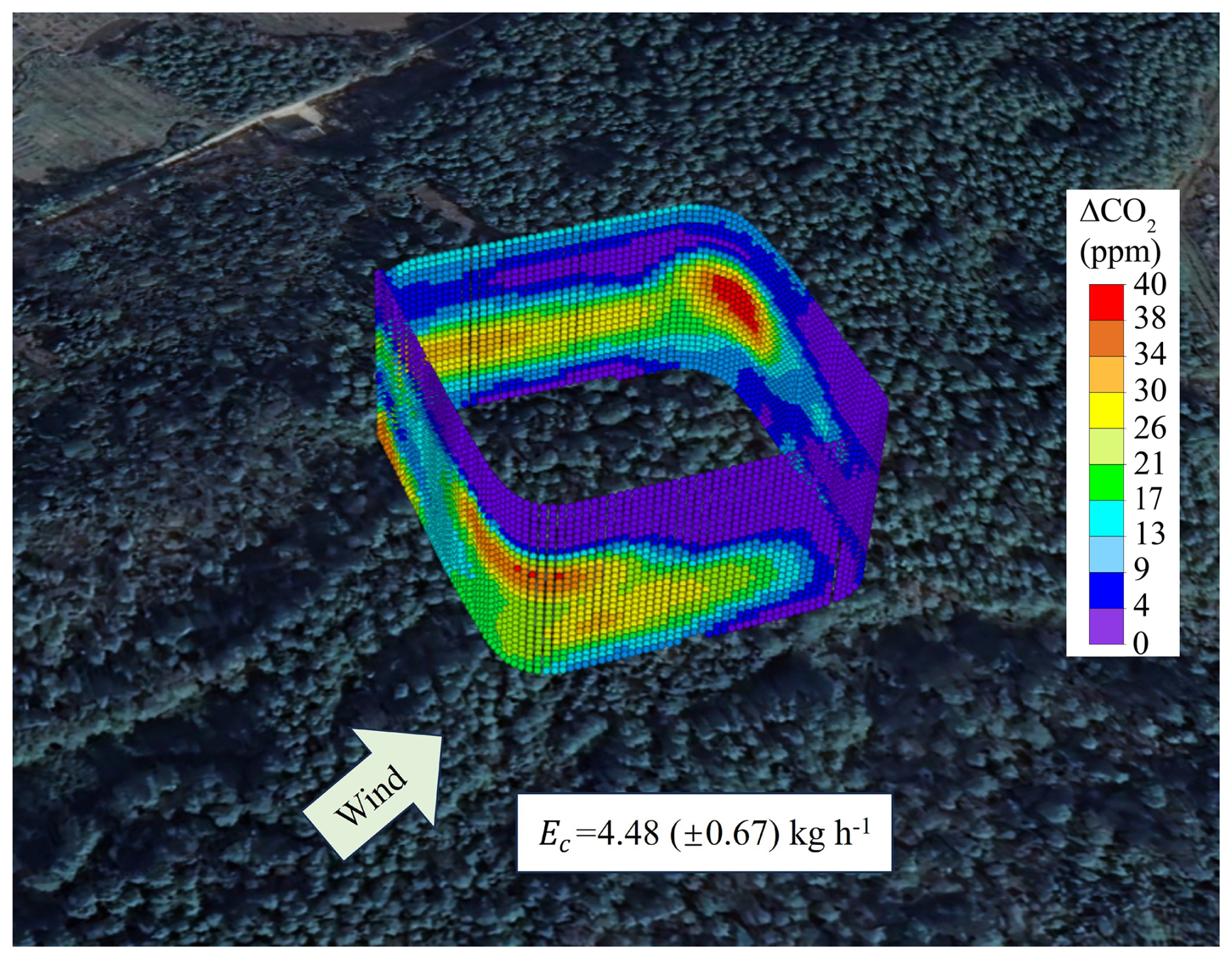
Figure 9 3-D distribution of the CO₂ mole fraction anomaly field (ΔCO₂), obtained from processed and interpolated UAV measurements following the procedure described in Sect. 2.3, within the 100 × 100 × 50 m³ domain during the morning flight on 8 August 2024, relative to a constant background value.

The wind vector shown in Fig. 9 indicates a prevailing southwesterly flow. The spatial alignment of the ΔCO₂ enhancements with the box boundaries suggests that lateral advection and flux divergence played a central role in shaping the observed CO₂ mole fraction gradients: CO₂-enriched air masses are transported into the control volume on the upwind side and redistributed along the walls, producing strong cross-boundary gradients that dominate the mass balance. Consistent with this interpretation, the box-mass balance calculation yields a positive net CO₂ emission rate of $E_{\mathrm{c}}=\mathrm{4.48}\pm \mathrm{0.67}$ kg h⁻¹ for the 100 × 100 × 50 m³ control volume. Decomposition of the individual mass-balance terms indicates that the horizontal advective contribution ($E_{\mathrm{C},\mathrm{H}}=\mathrm{4.22}\pm \mathrm{0.63}$ kg h⁻¹) accounts for nearly all of the net emission rate, whereas the vertical turbulent contribution is small ($E_{\mathrm{C},\mathrm{VT}}=\mathrm{0.26}\pm \mathrm{0.04}$ kg h⁻¹). The near-zero vertical term is also consistent with the concurrent EC observations similarly indicating a negligible turbulent vertical CO₂ flux. According to the sign convention defined in Sect. 3.2, the positive E_c indicates net outward CO₂ transport from the finite UAV sampling box, primarily resulting from horizontal flux divergence during this flight. This result should not be interpreted as the net CO₂ exchange between the entire forest ecosystem and the overall atmosphere, because the UAV box only encloses a limited area above the canopy. Instead, the box-based flux calculation is intended to quantify local CO₂ mass balance and to diagnose the contribution of horizontal advection, which can affect the interpretation and spatial representativeness of vertical CO₂ flux measurements.

Overall, the 3-D ΔCO₂ structure shown in Fig. 9 highlights that, at this moment, CO₂ exchange above the forest canopy was controlled predominantly by horizontal transport under heterogeneous CO₂ mole fraction fields. This highlights the importance of resolving spatial gradients and lateral boundary fluxes in order to diagnose horizontal advection and local CO₂ redistribution within the UAV sampling box. These processes can affect the interpretation and spatial representativeness of vertical flux measurements from a single-point flux tower, but they are not directly observable from the tower measurement alone.

4.4 Spatial heterogeneity of net CO₂ emission

To verify whether net emissions (E_C) calculated using the mass-balance approach differ across spatial scales, emission computations were made for three box-shaped control volumes constructed from the UAV flight tracks, with horizontal dimensions of 50 × 50 m², 100 × 100 m², and 150 × 150 m², respectively, and a common vertical extent of 50 m. The vertical contribution term E_C,VT and the horizontal transport contribution term E_C,H within each control volume were separately computed as per the detailed outlines above. In this analysis, E_C,H was calculated separately for each box size using the corresponding box-pattern boundary observations, whereas E_C,VT was derived from the paired vertical profile measurements collected during the same UAV flight. The net emissions were normalized by the areas of the boxes to give area-normalized emission intensity $e_{\mathrm{C}}=E_{\mathrm{C}}/A$, where A denotes the bottom area of the box. A total of 168 UAV flights were retained after quality control for the overall study. However, the number of observations within a specific season and time-of-day period was substantially smaller. Because the purpose of this analysis was to assess spatial-scale dependence, rather than seasonal or diurnal variability, only measurements obtained within the same season and time-of-day period were compared, thereby minimizing differences in ecosystem activity and atmospheric conditions. In addition, only cases with valid observations for all three control volume sizes (50 × 50 × 50, 100 × 100 × 50, and 150 × 150 × 50 m³) were retained to ensure an internally consistent comparison across spatial scales. After applying these criteria, seven observation days from summer noon and seven observation days from autumn morning were selected for the spatial-heterogeneity analysis. An observation day did not necessarily correspond to a single UAV flight; multiple UAV measurements could be conducted within the selected time window on the same day. These two periods also showed relatively good agreement between UAV-derived vertical fluxes and EC observations in Sect. 4.2.

For the seven selected summer noon observation days, UAV measurements were conducted between 13:00 and 14:00 LT (UTC$+\mathrm{08}:\mathrm{00}$) under predominantly southeasterly winds. The EC flux measurements corresponding to these UAV observation periods varied by less than 8 % among the seven selected days. Similarly, for the seven selected autumn morning observation days, UAV measurements were conducted between 06:00 and 07:00 LT (UTC$+\mathrm{08}:\mathrm{00}$) under predominantly southwesterly winds, and the corresponding EC flux measurements varied by less than 5 % among the seven selected days. These relatively small variations indicate that the selected observations within each season-time-period subset were obtained under broadly comparable ecosystem-exchange conditions. The selected datasets were intended to provide internally comparable subsets for evaluating spatial-scale dependence rather than to represent the full seasonal climatology.

If the CO₂ source-sink distribution in this region were spatially uniform, e_C would be expected to be similar among the three control volume sizes, i.e., e_C (150) ≈e_C(100) ≈e_C (50). For the seven selected summer noon observation days, the e_C were −0.25, −0.30, and −0.24 mg m⁻² s⁻¹ for the 50 × 50 × 50, 100 × 100 × 50, and 150 × 150 × 50 m³ control volumes, respectively (Fig. 10). These consistently negative values indicate net CO₂ uptake during the summer noon period, while the relatively small differences among the three spatial scales suggest weak scale dependence under these conditions. Furthermore, one-way analysis of variance (ANOVA) shows that the mean differences in e_C among the three scales were not statistically significant, with an ANOVA F-statistic of 0.349, indicating low between-group variance relative to within-group variance, and a p-value of 0.710, indicating that the observed differences could be readily explained by random variation rather than a true scale effect. Overall, under summer noon conditions, the area-normalized net exchange intensity is insensitive to the horizontal scales examined, and within-group variability dominates (Fig. 10).

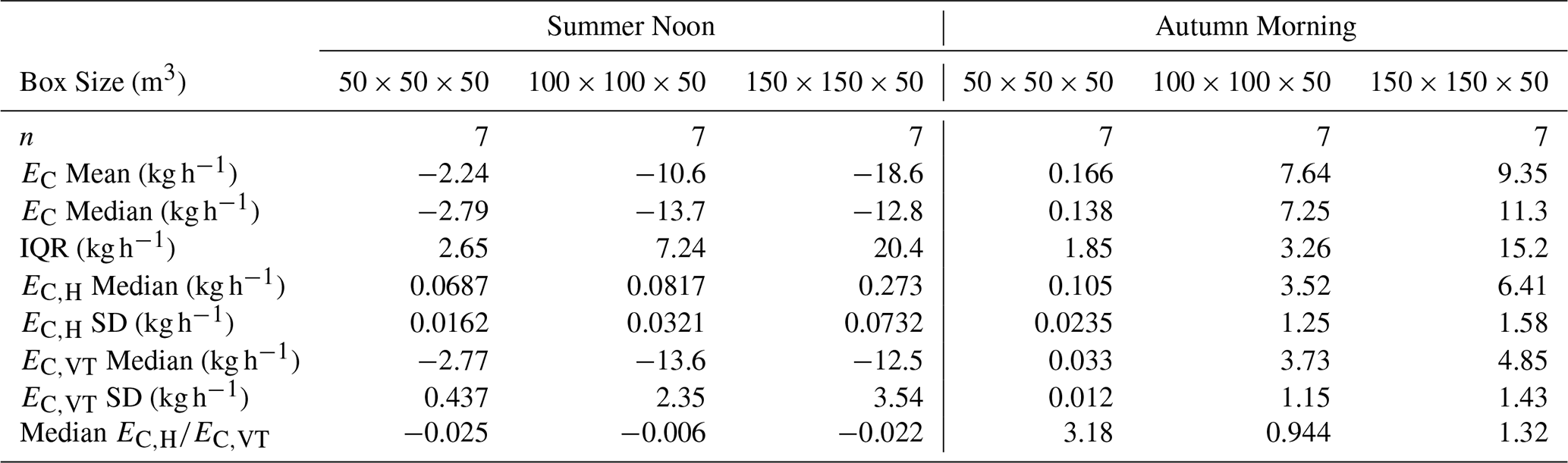
In addition, during summer at noon, the median values of $E_{\mathrm{C},\mathrm{H}}/E_{\mathrm{C},\mathrm{VT}}$ in Table 5 remain very small (from −0.025 to −0.006), indicating that the net CO₂ budget is dominated by the vertical turbulent-exchange term. This conclusion is further supported by the absolute magnitudes of the two components. For the 50 × 50 × 50, 100 × 100 × 50, and 150 × 150 × 50 m³ control volumes, the median E_C,H values were 0.0687, 0.0817, and 0.273 kg h⁻¹, respectively, whereas the corresponding median E_C,VT values were −2.77, −13.6, and −12.5 kg h⁻¹, respectively. Under summer noon conditions, stronger turbulence and more efficient vertical mixing likely suppress the relative influence of horizontal CO₂ gradients, so that horizontal transport contributes only a minor fraction to the virtual control volume budget. Although the negative values of $E_{\mathrm{C},\mathrm{H}}/E_{\mathrm{C},\mathrm{VT}}$ indicate that the horizontal and vertical components often have opposite signs, the magnitude of E_C,H remains much smaller than that of E_C,VT.

Figure 10 Distribution of e_C across box sizes (50 × 50 × 50 m³, 100 × 100 × 50 m³, 150 × 150 × 50 m³) during summer noon. Boxes represent the interquartile range (IQR), the center line is the median, and whiskers extend to 1.5 × IQR. Colored points are individual samples. The blue solid polyline connects the mean e_C of each group, with boxed numerical annotations. The reported F and p values denote the F-statistic and corresponding p-value from the one-way ANOVA, respectively.

Table 5 Summary statistics of net CO₂ emission estimates (E_C) derived from three box sizes during summer noon and autumn morning. For each box size, n denotes the number of valid samples. Reported metrics include the mean and median of E_C (kg h⁻¹), the interquartile range (IQR), the median and standard deviation (SD) of the horizontal-transport contribution (E_C,H) and the vertical-exchange contribution (E_C,VT), as well as the median ratio $E_{\mathrm{C},\mathrm{H}}/E_{\mathrm{C},\mathrm{VT}}$.

Another case study of spatial heterogeneity is based on the autumn morning dataset (Fig. 11). The mean values in Fig. 11 indicate that the emission intensities (e_C) derived for different box sizes (0.02, 0.21, and 0.11 mg m⁻² s⁻¹, respectively) differ to some extent. The differences among box sizes are substantially larger than the uncertainty of the method used in this study (30 %), representing differences in e_C among the different box sizes. One-way ANOVA also showed that the differences among the three scales were significant (F=4.482, p=0.025). This provides direct evidence that the net CO₂ emission intensity derived for the three virtual control volumes above the canopy is spatially heterogeneous.

Compared with the summer noon conditions, the role of horizontal transport becomes much more pronounced during autumn mornings. The median values of $E_{\mathrm{C},\mathrm{H}}/E_{\mathrm{C},\mathrm{VT}}$ increase to 3.18, 0.944, and 1.32 for the 50 × 50 × 50, 100 × 100 × 50, and 150 × 150 × 50 m³ control volumes, respectively. Importantly, these elevated ratios reflect not only the presence of horizontal CO₂ gradients, but also the fact that the vertical turbulent-exchange component is comparatively weak during this period. Specifically, for the 50 × 50 × 50, 100 × 100 × 50, and 150 × 150 × 50 m³ control volumes, the median E_C,H values were 0.105, 3.52, and 6.41 kg h⁻¹, respectively, whereas the corresponding median E_C,VT values were 0.033, 3.73, and 4.85 kg h⁻¹, respectively. This indicates that, under weak-turbulence morning conditions, horizontal CO₂ transport can become comparable to, or even exceed, the vertical turbulent component. Such behavior is consistent with enhanced spatial heterogeneity in CO₂ exchange across the different control volumes. As the control volume scale increases, small-scale horizontal gradient structures are progressively averaged out, reducing the relative contribution of E_C,H and leading to the observed scale dependence of E_C. The component-wise contribution analysis (Table 5) indicates that the relative contribution of the horizontal transport term is markedly enhanced. The median metric, median $E_{\mathrm{C},\mathrm{H}}/E_{\mathrm{C},\mathrm{VT}}$, is 3.18 for 50 × 50 × 50 m³, 0.944 for 100 × 100 × 50 m³, and 1.32 for 150 × 150 × 50 m³. These results suggest that there is significant spatial heterogeneity in the CO₂ emissions/uptake in the range covered by the different boxes leading to horizontal CO₂ mole fraction gradients, and as a result near-surface horizontal CO₂ gradients under the measured horizontal winds are non-negligible within small control volumes.

This scale sensitivity further highlights the true advantage of UAV observations for characterizing spatial heterogeneity. UAV measurements can provide multipoint, 3-D CO₂ distributions and associated wind speed gradient information within a short time window, enabling the simultaneous estimation of E_C,H (horizontal transport) and E_C,VT (vertical transport) within a consistent data framework. Moreover, by varying the box sizes, the same dataset can be re-aggregated into different spatial scales to facilitate a multi-scale comparison. In contrast, EC flux towers essentially measure point-based vertical turbulent fluxes, whose representativeness is determined by a footprint that varies with wind direction and atmospheric stability. As a result, flux tower observations yield a footprint-weighted effective flux, making it difficult to construct a spatial control volume and impossible to explicitly resolve the lateral transport term E_C,H. Therefore, box-size dependence driven by spatial heterogeneity is more readily captured by UAV observations, whereas flux towers are limited in both observation geometry and the types of physical quantities they can diagnose.

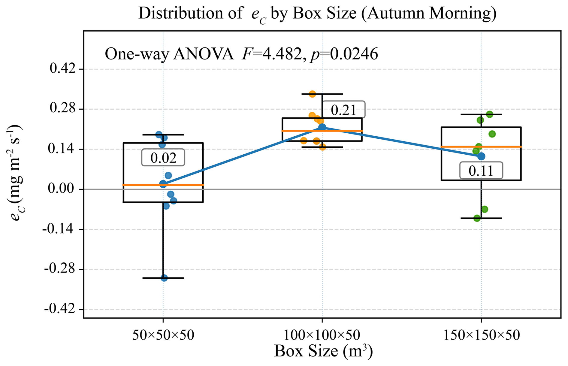
Figure 11 Distribution of e_C across box sizes (50 × 50 × 50 m³, 100 × 100 × 50 m³, 150 × 150 × 50 m³) during autumn morning. Boxes represent the interquartile range (IQR), the center line is the median, and whiskers extend to 1.5 × IQR. Colored points are individual samples. The blue solid polyline connects the mean e_C of each group, with boxed numerical annotations. The reported F and p values denote the F-statistic and corresponding p-value from the one-way ANOVA, respectively.

5 Conclusions

This study developed and field-evaluated a methodology for quantify 3-D CO₂ fluxes over a forest ecosystem using an integrated unmanned aerial vehicle measurement platform, a specifically designed flight strategy, and a computational algorithm that explicitly resolves both vertical exchange and horizontal advection within a unified 3-D mass-balance framework. Extensive applications of this methodology at the Qianyanzhou subtropical plantation forest site demonstrate that the methodology can robustly determine canopy-scale CO₂ exchange. Vertical CO₂ fluxes derived from the airborne profiles are in good agreement with those determined from collocated eddy covariance tower observations across seasons, with a Pearson correlation coefficient of r=0.9 based on 168 paired samples, indicating that the UAV-based gradient method reproduces both the magnitude and variability of vertical turbulent exchange under typical daytime conditions. The profile-derived vertical fluxes showed clear diurnal and seasonal patterns over the forest ecosystem at Qianyanzhou, with the strongest uptake around midday during the growing season and near-neutral exchange in winter. However, the vertical fluxes derived from the airborne profiles and those determined from the eddy covariance measurements diverged under weak turbulence conditions during the stable evening period, highlighting increased uncertainties in both methods under low vertical flux conditions.

Measurements collected along the box-pattern flight paths further reveal that horizontal transport can be a dominant term under certain conditions. Enhanced CO₂ mole fractions on the virtual walls of the flight boxes and wind vectors show pronounced spatial heterogeneity and lateral gradients, especially in the morning, indicating that advection-driven convergence/divergence may substantially shape the CO₂ mass balance within the airborne-defined control volume above the forest canopy, processes that cannot be directly resolved from single-tower measurements. A multi-scale analysis using different box sizes (50 × 50 × 50, 100 × 100 × 50, and 150 × 150 × 50 m³) shows that net emission estimates can exhibit scale dependence, reflecting the spatial heterogeneity of sources/sinks. These results highlight the value of airborne observations for determining spatial heterogeneity in short-term ecosystem carbon exchange with the atmosphere, a task that is difficult to accomplish using single-site measurements alone, for diagnosing when and where the assumption of horizontal homogeneity becomes invalid, and for quantifying lateral flux contributions explicitly. The horizontal flux analysis should therefore be interpreted as a diagnostic of local advective redistribution and spatial representativeness above the canopy, not as a measure of whole-forest lateral CO₂ export or import.

Overall, the combined box-profile airborne framework provides a flexible and spatially explicit complement to conventional eddy covariance monitoring, offering an effective pathway to bridge the observational gap between point-scale tower fluxes and larger-scale heterogeneities, particularly over heterogeneous canopies and complex terrain. In conclusion, unmanned aerial vehicle platforms offer a transformative opportunity for observing ecosystem-atmosphere CO₂ exchange in 3-D. With continued methodological refinement and broader application, such systems are well positioned to become an essential component of next-generation carbon observation strategies in forest ecosystems and beyond.