Characterising the occurrence of monomodal and multimodal ice hydrometeor populations and their fall speeds in midlatitude frontal ice clouds using radar Doppler spectra

Multimodality in vertically pointing radar Doppler spectra is frequently observed in stratiform clouds, but understanding the microphysical processes causing these signatures, and indeed quantifying their occurrence, remains a challenge. In this study, we utilise Ka-band radar Doppler spectra from 23 deep stratiform clouds observed over Chilbolton, UK. We apply a peak finding algorithm to identify spectral reflectivity peaks in the Doppler spectra, which can be used to infer the presence of distinct coexisting ice particle populations, such as pristine crystals mixed with aggregate snowflakes. Using these results, we provide a quantitative estimate for the distribution of multimodal spectra with temperature. There are two clear temperature regimes where the occurrence of multimodal spectra increases sharply, indicating production of new particles; these are between −8 and −3 °C, which we attribute to secondary ice production, and between −18 and −13 °C, where the mechanism responsible for producing multimodal spectra is unclear.

The peak finding algorithm also returns the velocities associated with the peaks in spectral reflectivity, which allows us to analyse the distribution of velocity with temperature for primary and secondary particle populations. We find that primary populations from monomodal spectra experience a significant reduction in vertical velocity at −13 °C. Examining the mean Doppler velocity (MDV) reveals a decrease in MDV from monomodal spectra at the same temperature. Whilst it has been suggested previously that this velocity decrease is caused by the presence of a secondary mode, our findings indicate that it is governed by the primary population; that is, falling particles are slowing down. Dendritic growth is favoured near this temperature, and we therefore hypothesise that particles such as polycrystals and aggregates, which form in colder cloud layers, precipitate to this level and form dendritic branches. This velocity decrease may then be associated with increased drag force acting against these particles which counteracts their increasing mass, thus causing the velocity to decrease.

1 Introduction

Although only a small fraction of global precipitation reaches the surface as snow, satellite observations have shown that the majority of precipitation events originate from the ice phase (Field and Heymsfield, 2015; Heymsfield et al., 2020). Ice microphysical processes also have a significant influence on radiative balance due to the interaction of ice crystals with solar radiation; studies have suggested that changing particle habits, phase and size distributions are likely to have noticeable climate impacts (Hofer et al., 2019; Zhang et al., 2022; Pasquier et al., 2023). Uncertainties in how ice microphysical processes will change in both ice and mixed phase clouds are responsible for some of the greatest uncertainties in future climate predictions (Sun and Shine, 1994; Lohmann and Feichter, 2005; Sherwood et al., 2020; Mülmenstädt et al., 2021). This motivates continual improvement in our understanding of ice microphysical processes and their representation in both numerical weather prediction (NWP) and climate models. Interpreting remote sensing observations is also dependent on our fundamental understanding of ice microphysical processes and characteristics.

Accurate representation of ice particle size distributions (PSDs) remains a challenge. Early attempts to characterise the shape of ice PSDs (Gunn and Marshall, 1958) involved estimating the size of aggregate snowflakes by analysing the diameter of a water drop produced by a singular melted snowflake. From these experiments, Gunn and Marshall (1958) concluded that aggregate snowflakes greater than 1 mm in diameter are well represented by an exponential distribution. More recent studies using aircraft observations (e.g. Evans et al., 2005; Woods et al., 2008) have shown concurring results that the tail of ice PSDs is exponential. However, other studies based on in situ PSD measurements (e.g. Heymsfield et al., 2002, 2013; Leighton et al., 2020) suggest that gamma distributions are a more accurate representation of observed ice PSDs. Understanding the shape of ice PSDs is essential to their accurate representation in NWP models, but the complexity of ice microphysical properties and processes has necessitated simplifications regarding PSD shape in parameterisations (Bartolomé García et al., 2024). As a result, PSD parameterisations are unable to accurately represent multimodal particle populations. Mammatt et al. (2026) demonstrate this using aircraft observations to evaluate the accuracy of the double moment gamma parameterisation from the Cloud and AeroSol Interacting Microphysics (CASIM) scheme (Field et al., 2023), which has recently been implemented in the operational UK Met Office Unified Model. Examination of the observed PSDs, particle images and particle shape analysis showed that the PSD shape was likely to have been influenced by secondary ice production (SIP), leading to a bimodal PSD. This led to poor representations of the observed PSDs, as the parameterisation could not simultaneously fit the high concentration of relatively small particles produced by SIP as well as the lower concentration of relatively large particles. This resulted in large errors in forecast process rates, including underestimating aggregation rate by up to 50 % and precipitation rate by up to 25 %. The analysis in Mammatt et al. (2026) is based on one case study, but demonstrates the importance of accurately representing ice PSDs in NWP models and how multimodal populations can impact that representation. It is therefore desirable to look at a larger dataset to better understand how frequently and at what temperatures bimodal PSDs are observed. In the present study, this will be achieved by identifying spectral reflectivity peaks in vertically pointing radar Doppler spectra, from which the presence of multimodal PSDs can be inferred, along with the vertical velocity of these populations. Gathering statistics over many events will allow us to quantify the occurrence of multimodal spectra and of the velocity of different particle populations with temperature. The aim is to contribute to improving interpretation of the microphysical processes active at different temperatures, which may be used to inform representations of ice microphysical processes in NWP models and analysis of remote sensing retrievals in the future.

Vertically pointing radar Doppler spectra provide information on particle vertical velocities with altitude. From these observations, it is possible to identify coexisting particle populations which are distinguishable by their velocities (Kollias et al., 2002; Luke and Kollias, 2013; Kneifel et al., 2016). The terminal velocity of large unrimed snowflakes generated by aggregation is almost independent of particle size, as the additional drag caused by the larger cross-sectional area opposes the effect of increasing mass (Kneifel and Moisseev, 2020). From in situ and radar observations, there is evidence to suggest that this terminal velocity is about 1 m s⁻¹, assuming surface pressure and negligible vertical air motion (Zawadzki et al., 2001). The high concentrations of secondary particles produced by SIP are distinguishable from the primary population due to their very slow vertical velocities (Shupe et al., 2004; Kalesse et al., 2016; Field et al., 2017). Riming, on the other hand, increases the vertical velocity of particles relative to an unrimed population due to their increased mass and fall characteristics (Zikmunda and Vali, 1972; Locatelli and Hobbs, 1974; Mosimann, 1995). It is therefore possible to segregate coexisting particle populations observed in Doppler spectra due to differing fall speeds, and to suggest microphysical processes which may be active and result in differing velocities. This feature has allowed previous studies (e.g. Oue et al., 2018; Wugofski and Kumjian, 2025) to utilise peak separation methods to identify cloud where multiple populations of particles are present. It is also important to remember that distinct particle populations with different characteristics can have vertical velocities which are indistinguishable in the Doppler spectra; these populations can cause the Doppler spectrum to broaden without producing a separate peak. Previous studies investigating drizzle formation have used the skewness of Doppler spectra to identify early drizzle generation (Kollias et al., 2011b, a; Luke and Kollias, 2013), but to the best of our knowledge, similar methods for early identification of multimodal ice populations have not been studied. However, von Terzi et al. (2022) suggest that skewness is one of the variables which reacts earliest (i.e. at the coldest temperatures) to new particle formation near the dendritic growth layer (DGL, −10 to −20 °C). This might suggest skewness is particularly sensitive to changes in the shape of the ice particle velocity and size distributions.

Ice multiplication influences the shape of observed Doppler spectra by forming populations of particles with slow vertical velocities. It has long been observed that concentrations of ice nucleating particles (INPs) can be many times lower than observed concentrations of ice crystals in clouds (e.g. Mossop, 1985; Harris-Hobbs and Cooper, 1987; Pruppacher and Klett, 1997; Cantrell and Heymsfield, 2005). Early observations of this discrepancy (e.g. Mossop et al., 1970, 1972) prompted investigation into mechanisms to explain these observations; these have included amplification of primary nucleation (e.g. Hobbs and Rangno, 1985; Fridlind et al., 2007) and, more convincingly, production of ice crystals without requiring an INP (Field et al., 2017, and references therein). SIP has therefore been a topic of interest for a number of years. Generally, however, studies have focussed on SIP in convective clouds, with relatively little attention paid to stratiform frontal clouds. Hallett and Mossop (1974) first showed findings consistent with the production of secondary ice particles that result from the splintering of a liquid cloud droplet during the riming process. These splinters are initially very small but as they grow in both size and mass, they appear as a secondary particle mode in radar Doppler spectra, which is distinguishable from the primary population by their slow vertical velocity (Zawadzki et al., 2001). Hallett and Mossop (1974) suggest that rime splintering is observed to be active in a relatively narrow temperature regime of approximately −3 to −8 °C. Since this first study, there have been numerous studies further investigating this process using in situ aircraft observations (Crosier et al., 2011, 2014; Lloyd et al., 2014; Keppas et al., 2017). However, results from recent laboratory studies suggest there are still discrepancies regarding the efficiency of this mechanism (Seidel et al., 2024). Droplet fragmentation has also been investigated as a mechanism of generating secondary particles (Phillips et al., 2018), which is thought to require drizzle drops of at least 50 µm (Wildeman et al., 2017) but may be more efficient for larger drops of > 300 µm (Lauber et al., 2018; Keinert et al., 2020). A recent study by Pfeifer et al. (2025) showed observations supporting the idea that fragmentation of refreezing raindrops is likely to be an efficient ice multiplication mechanism. Ice-ice collisional breakup has also been proposed as an efficient SIP mechanism (Vardiman, 1978; Yano and Phillips, 2011; Yano et al., 2016; Phillips et al., 2017), in which ice fragments are produced during collisions between ice particles. Whilst there is a lack of agreement surrounding the conditions in which the droplet fragmentation and ice-ice collisional breakup mechanisms are active, they may occur over a broader temperature range than rime splintering (Field et al., 2017; Korolev and Leisner, 2020).

This study will be presented as follows: in Sect. 2, we describe the radar and model data used and explain the processing of the spectral data. In Sect. 3, we explain the peak finding algorithm used to identify spectral reflectivity peaks in the Doppler spectra and how the parameters for the algorithm were chosen and validated. We assess the turbulent contribution to the spectral width and explain the impact this has on the accuracy on the peak finding algorithm, filtering out data which is impacted. In Sect. 4, we apply the method to 23 case studies and use the results from the peak finding algorithm to quantify how frequently multimodal spectra are observed in radar Doppler spectra as a function of temperature. We suggest that rime splintering causes the high percentage of observed multimodal spectra at −5 °C, but also show findings consistent with the production of secondary particles in a second temperature window of −10 to −18 °C. The mechanism for this is unclear. We then investigate the distributions with temperature of particle population velocity and mean Doppler velocity (MDV), and how these differ between monomodal and multimodal microphysical regimes. To our knowledge, there are limited studies in the existing literature quantifying the fraction of multimodal spectra with temperature in frontal clouds and which demonstrate the impact of multimodal cloud regimes on Doppler radar measurements.

2 Data

2.1 Radar data

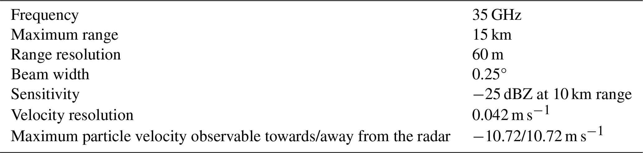
The Copernicus Ka-band (35 GHz) radar at the Chilbolton Facility for Atmospheric and Radio Research (CFARR) takes continuous routine observations, including reflectivity, MDV, standard deviation of mean Doppler velocity (${\mathit{\sigma }}_{\stackrel{\mathrm{‾}}{v}}$) and spectral width (Walden, 2026). It also takes observations of Doppler spectra every minute; it is important to note that these are 1 s spectra recorded once per minute, and are not an average over several seconds. Key properties of the radar are summarised in Table 1 (see also Illingworth et al., 2007). Note that here and throughout this study, negative velocities indicate movement towards the radar, and therefore indicate descending hydrometeors for our vertically pointing radar. Increases or decreases in velocity will be discussed in the absolute sense whilst retaining the negative sign convention.

Table 1 Summary of key properties of the Copernicus radar.

Using archived data, we identify 23 frontal case studies from a 14-month period in 2017–2018 to examine in closer detail; Table 2 provides further detail on each of these cases and more information for each case can be found in the Supplement. The cases were chosen by looking for nimbostratus cloud systems in the daily radar quicklook plots, and comparing those events with features marked on the operational Met Office surface pressure analysis charts. The analysed cases were selected to represent typical frontal clouds, and are primarily stratiform with large vertical extents covering a wide range of temperatures, and surface precipitation for part of the observation period. Data from all 24 h of each case study day are included in the analysis that follows. Reflectivity, example spectrograms, and results from the peak finding method (see Sect. 3.1) are shown for each case in the Supplement. Data are received in their raw, uncalibrated form, and therefore noise correction and calibration methods must be applied before further analysis is carried out. Corrections to reduce the impact of signal attenuation by rain and turbulent Doppler spectra broadening are also applied. These processes are explained in the following sections.

Table 2 Description of the case studies selected to examine in further detail in our analysis. Depth of system is estimated to within 0.5 km from visual examination of radar images, and refers to the depth above the melting layer. Cloud top temperatures are estimated to within 5 °C from comparison between radar images and model data (see Sect. 2.2). Multimodal occurrence refers to the percentage of all in-cloud pixels which are identified as multimodal. Maximum surface rain rates are those associated with the main deep frontal cloud observed on each day, and were measured with a high resolution rain gauge (Norbury and White, 1971) at CFARR. Descriptions of the synoptic situation are based on surface pressure analysis charts from the UK Met Office, and highlight the features that cloud is associated with.

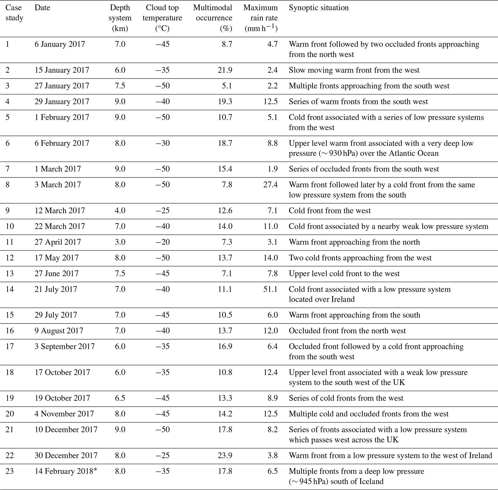
^* Detailed analysis of aircraft data for this case can be found in Mammatt et al. (2026).

2.1.1 Noise correction

To extract the main spectral reflectivity peak and remove artefacts caused by echoes, we apply noise correction to the spectral data. This is achieved by estimating the mean background noise value, P_noise, from the uncalibrated power of the signal of the signal, P_u. This involves calculating the mean spectral power of empty gates; the standard deviation of the power in these empty gates is also calculated. P_noise is then subtracted from the remaining spectra and data within three standard deviations of P_noise are removed. This method allows us to retain the vast majority of the observed spectra, even at low reflectivities. This is important for providing information on the slow-moving (and therefore weakly scattering) ice particles. At this stage, the data are still in their uncalibrated form, so the next step is to apply a calibration. We also apply a range correction which accounts for the decrease in echo power with range for a given reflectivity, which is

$$\begin{array}{}\text{(1)}& Z_{\mathrm{c}}=P_{\mathrm{u}}+\mathrm{20}{\log }_{\mathrm{10}}\left(R\right)-C_{\mathrm{calibration}}\end{array}$$

where Z_c is the calibrated reflectivity, P_u is the uncalibrated power of the signal, and C_calibration is a calibration constant; Z_c, P_u and C_calibration are all in dB units. R is the range in metres. The Copernicus radar is routinely calibrated by comparing the signal to that from the Chilbolton Advanced Meteorological Radar (CAMRa), which operates in the S-band (3 GHz) and is absolutely calibrated to within ±0.5 dB in Rayleigh scattering cirrus clouds. We follow the procedure outlined in Hogan et al. (2000). CAMRa is calibrated in heavy rain using the redundancy between reflectivity, differential reflectivity and differential phase shift, as described in Goddard et al. (1994). 35 GHz reflectivity profiles are then matched with the calibrated 3 GHz data in high level cirrus clouds where the particles are Rayleigh scatterers at both 35 and 3 GHz. The small gaseous attenuation at 35 GHz is taken into account by using numerical forecast output for the water vapour profile of the atmosphere, and a line-by-line absorption model (Liebe, 1989).

Figure 1 shows an example of a noise-corrected spectrogram (stacked Doppler spectra with height); this example is from 17 May 2017. Figure 1a shows the full spectrogram; there is a sharp increase in the observed Doppler velocities and range of velocities at approximately 3 km, which is because rain falls significantly faster than ice particles (Field et al., 2005). The primary mode is falling at approximately −0.7 to −1.5 m s⁻¹, and there are two regions at higher altitude where signatures consistent with multimodality are visible, which can be seen in closer detail in Fig. 1b. At 3–4 and 5–6 km, we see that there are two “strands” to the spectrogram, which is indicative of the formation of a particle population which has distinctly different properties to the primary population.

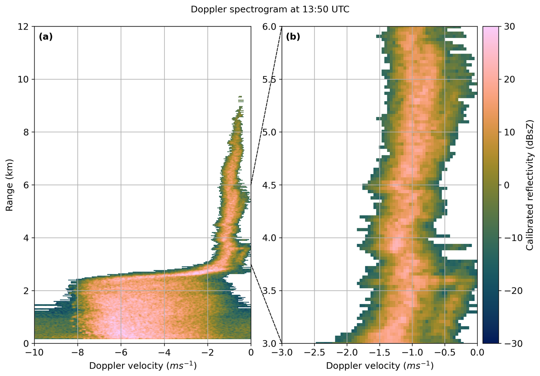
Figure 1 An example of the routine Doppler spectra observed at CFARR. This example is from 13:50 UTC on 17 May 2017. Negative velocity values indicate movement towards the radar. Panel (a) shows the full spectrogram and panel (b) shows a closer view of the ice phase regions of the spectrogram where multimodal spectra are present.

2.1.2 Assessing the effect of turbulence on Doppler spectra

Due to the stratiform nature of the cases selected for this study, we expect that the primary influence on the observed Doppler spectra will be particle fall speeds. However, turbulence also acts to broaden the Doppler spectra (Babb et al., 2000). To assess the impact of air turbulence on the observed Doppler spectra examined, we follow the technique described in O'Connor et al. (2005) to quantify the contribution of turbulence to the width of our observed spectral peaks. The broadening of the Doppler spectrum due to homogeneous isotropic turbulence is

$$\begin{array}{}\text{(2)}& {\mathit{\sigma }}_{\mathrm{t}}^{\mathrm{2}}={\mathit{\sigma }}_{\stackrel{\mathrm{‾}}{v}}^{\mathrm{2}}{\displaystyle \frac{L_{\mathrm{s}}^{\frac{\mathrm{2}}{\mathrm{3}}}}{L_{\mathrm{t}}^{\frac{\mathrm{2}}{\mathrm{3}}}-L_{\mathrm{s}}^{\frac{\mathrm{2}}{\mathrm{3}}}}},\end{array}$$

where ${\mathit{\sigma }}_{\stackrel{\mathrm{‾}}{v}}$ is the standard deviation of the mean Doppler velocity over a time window (in our case this time window is 30 s). L_s and L_t are the length scales for spectral and moment level observations respectively. The length scale L is calculated by

$$\begin{array}{}\text{(3)}& L=Ut+\mathrm{2}z\sin \left({\displaystyle \frac{\mathit{\theta }}{\mathrm{2}}}\right),\end{array}$$

where t = 1 s for L_s and t = 30 s for L_t, corresponding to the sampling time of a single MDV estimate versus the window for computing ${\mathit{\sigma }}_{\stackrel{\mathrm{‾}}{v}}$. U is the horizontal wind speed, z is the height in metres and θ is the beamwidth of the radar in radians (see Table 1).

Figure 2 shows an example of the quantities involved in these calculations. Figure 2a shows the standard deviation of mean Doppler velocity from the moment level observations. Figure 2b shows the magnitude of the horizontal wind speed, calculated from the zonal and meridional model winds (see Sect. 2.2). Figure 2c shows the turbulent contribution to spectral width, calculated using the method outlined above. In this example, we see that the turbulent contribution to the spectral width is generally very low throughout the majority of the cloud, with values generally below 0.05 m s⁻¹. There is a region at around 13:00 UTC where there is a significant increase in σ_t, with values in excess of 0.2 m s⁻¹. This indicates that turbulent processes in this region of the cloud act to broaden the observed Doppler spectra here. The turbulent contribution to spectral width is calculated for each of our case studies; from examination of these results and comparisons with individual spectra from all cases, we choose a threshold of 0.042 m s⁻¹ (equal to one velocity bin in our Doppler spectrum) and remove data where the turbulent contribution is greater than this threshold. This threshold is fixed and is not recalculated for each case. Ice microphysical processes happen at low fall speeds so sensitivity to small velocity changes from external factors is high; this has impacts for further analysis, such as identifying individual populations and mechanisms. Our conservative velocity threshold removes these effects, whilst allowing the vast majority of data to be kept.

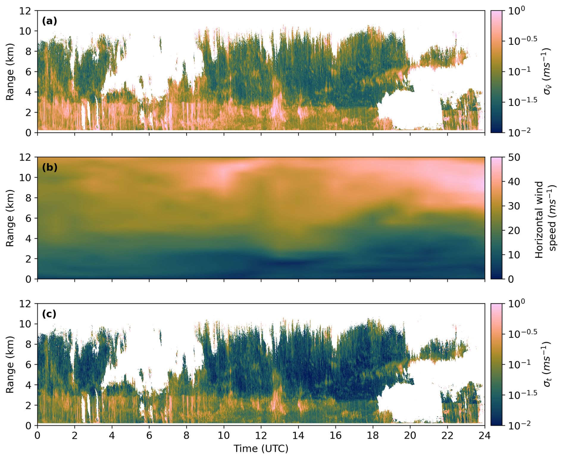
Figure 2 Panel (a) shows the standard deviation of mean Doppler velocity, ${\mathit{\sigma }}_{\stackrel{\mathrm{‾}}{v}}$, from the moment level observations. Panel (b) shows the magnitude of the horizontal wind speed from the model. Panel (c) shows the turbulent contribution to spectral width, σ_t, estimated using the method described in Sect. 2.1.2 for the cloud volume observed on 17 May 2017.

2.1.3 Impact of rain attenuation

Attenuation of radar signals by raindrops results in weakened echoes. The key results presented in the following sections are not sensitive to attenuation, as it does not influence the shape of the spectra but simply causes a reduction in the reflectivity across the whole spectrum. It is possible, however, that high levels of attenuation may cause spectral peaks with lower spectral reflectivities to fall below the noise floor and thus be removed; it is therefore desirable to identify and neglect regions which are heavily influenced by attenuation. Rain rate is measured at CFARR using a high resolution rain gauge (Norbury and White, 1971), and we can use this to estimate attenuation of the radar signal strength caused by rain. One-way attenuation for a Ka-band radar is given by

$$\begin{array}{}\text{(4)}& a\approx \mathrm{0.28}R\end{array}$$

(Matrosov, 2005), where a is the attenuation (in dB km⁻¹) and R is the rain rate (in mm h⁻¹). Using the 0 °C isotherm from the model (see Sect 2.2), the total attenuation caused by rain below the melting layer is estimated. We can also estimate attenuation caused by the melting layer for a Ka-band radar using the relationship described in Li and Moisseev (2019), which is

$$\begin{array}{}\text{(5)}& A=\mathrm{0.97}{R}^{\mathrm{0.61}}\end{array}$$

where A is the attenuation caused by the melting layer in dB.

Figure 3a shows the radar image calculated from the integrated Doppler spectra, Fig. 3b shows the estimated attenuation caused by rain, Fig. 3c shows attenuation caused by the melting layer, and Fig. 3d shows the total attenuation estimate (the sum of attenuation caused by rain and the melting layer). The blue shading in all panels shows where the total attenuation exceeds 10 dB. Comparing Figs. 3b and c shows that the majority of the total attenuation is caused by rain. We can see that the peak of ∼ 36 dB of total attenuation seen at around 13:00 UTC corresponds to an apparent drop in cloud top height, to around 6 km from approximately 10 km at neighbouring times; we suggest that this reduced echo top is in fact a result of weakened signal rather than a physical feature. To remove the influence of events like this, we exclude regions of cloud where the total attenuation estimate exceeds 10 dB.

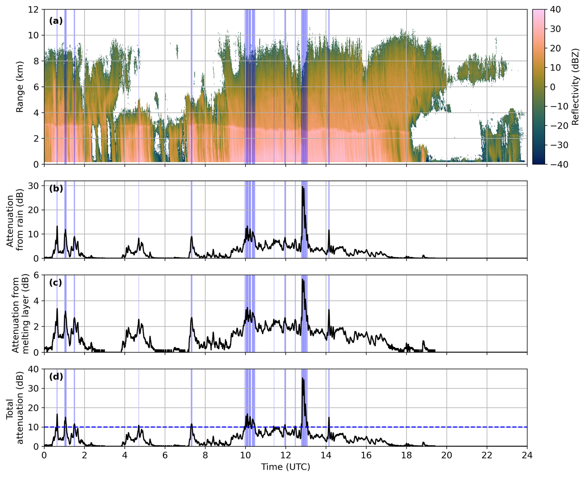
Figure 3 Radar image calculated from integrated Doppler spectra (a), attenuation from rain (b), attenuation from the melting layer (c) and total attenuation (d) for the example case. The blue shading in all panels shows where the total attenuation exceeds 10 dB. Note the differing y-axis scales between panels (b), (c) and (d).

2.2 Model data

Archived NWP model data for Chilbolton for each case was obtained via the ACTRIS Cloudnet portal. ICON model data (Zängl et al., 2015) is available for cases from 6 January to 17 May 2017, which has a lead time of 12–23 h, and ECMWF IFS data (Wedi et al., 2015) is available for cases from 27 June 2017 to 14 February 2018, which has a lead time of 12–35 h. Variables are forecast hourly in both models. Here, we are primarily interested in temperature from the models so that comparisons can be made with the location of different microphysical features. As our cases are associated with extratropical cyclones, they do not have fine scale temperature fluctuations, so hourly forecast temperatures are sufficient. Mittermaier and Illingworth (2003) compared the height of the 0 °C isotherm from modelled hourly temperature profiles against the height of the bright band for several frontal cases, and found that models were able to capture of the height of the bright band and the shape of the frontal surface mainly with very good accuracy. Comparison between the height of the bright bands with that of the 0 °C isotherm in our cases showed similarly good agreement, and it is therefore likely that differences between the modelled and true atmospheric temperature are not introducing large uncertainties into our results. Doppler spectra measurements are made every minute; we therefore interpolate the temperature field onto the same grid so that we have a temperature profile for every Doppler spectrogram. The horizontal wind fields are also used as inputs to Eq. (2).

3 Methods

There have been several different methods developed for identifying peaks in Doppler spectra. These include identifying peaks separated by the noise floor (Hildebrand and Sekhon, 1974) and utilising spectral density sorting algorithms (Kollias et al., 2007). More recently, Kalesse et al. (2019) developed a supervised machine learning method that is first trained on manually identified peaks before being used to identify peaks in the Doppler spectra. Radenz et al. (2019) created an algorithm that transforms the Doppler spectrum into a tree structure, with each peak represented as a node within the tree. Combining these methods facilitates the use of both to identify peaks and gain additional information about the microphysical properties of each particle mode (Vogl et al., 2024). Whilst these methods are invaluable for providing detailed microphysical information on selected case studies, a more computationally efficient method is desirable to process data from several cases.

3.1 Doppler spectra peak finding algorithm

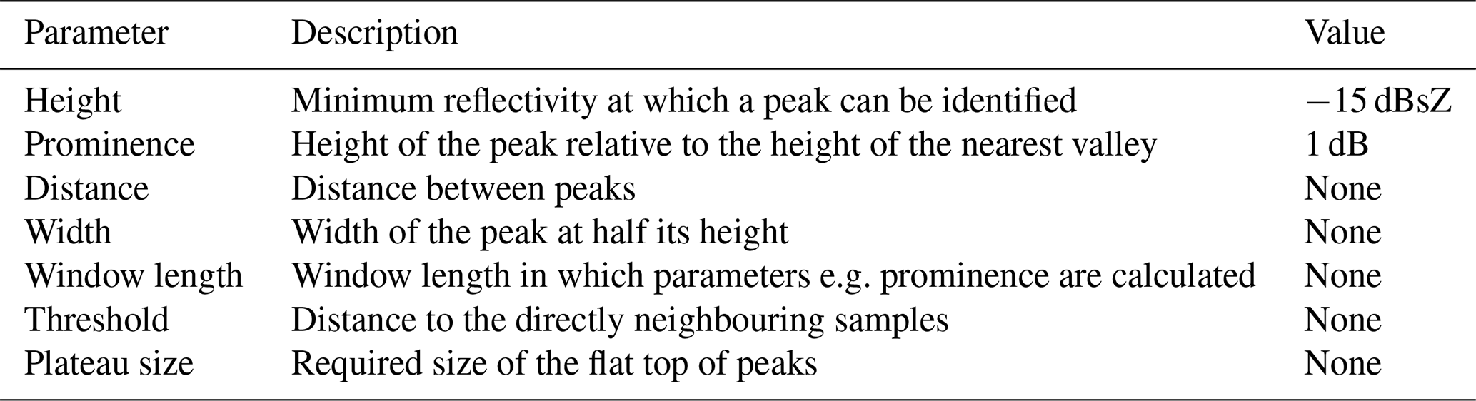
In order to quantify the fraction of multimodal spectra in our case studies, we identify the number of peaks in the one dimensional Doppler spectra at each time and height gate (hereafter referred to as “pixels”). It is unrealistic to manually identify the spectral peaks in each of the 15.9 million pixels examined in this study, so we apply a peak finding algorithm to the one dimensional Doppler spectra. We use the SciPy function “find_peaks” (Virtanen et al., 2020) to identify peaks in spectral reflectivity. This function was chosen because SciPy is designed to efficiently process large quantities of data. Section 3.1.1 and Table 3 describes the tuneable parameters in the “find_peaks” functions in more detail and how they were chosen, and Sect. 3.1.2 describes how we validate the accuracy of the peak finding parameters.

Table 3 Description of the parameters from SciPy's peak finding algorithm (Virtanen et al., 2020) and the values chosen. Parameters with a value of “None” were not used in this method.

3.1.1 Choosing peak finding parameters

The tuneable parameters and values chosen for the “find_peaks” function are outlined in Table 3. Height determines the minimum spectral reflectivity at which a peak can be identified; the low threshold chosen here was purely to remove any remaining noise that had not been removed during the noise correction process (described in Sect. 2.1.1). The method for finding the prominence of peaks is demonstrated using idealised spectra in Fig. 4. Prominence is found by extending a horizontal line in both directions from the top of a peak until it intersects with the slope of a higher peak or the edge of the spectrum, shown as the red dotted lines in Fig. 4. The difference between the lowest signal value between these two points and the height of the peak is the prominence, shown by the blue dashed line in this figure. Changing the prominence threshold changes the minimum length of the blue line whilst still retaining this maximum as a distinct peak.

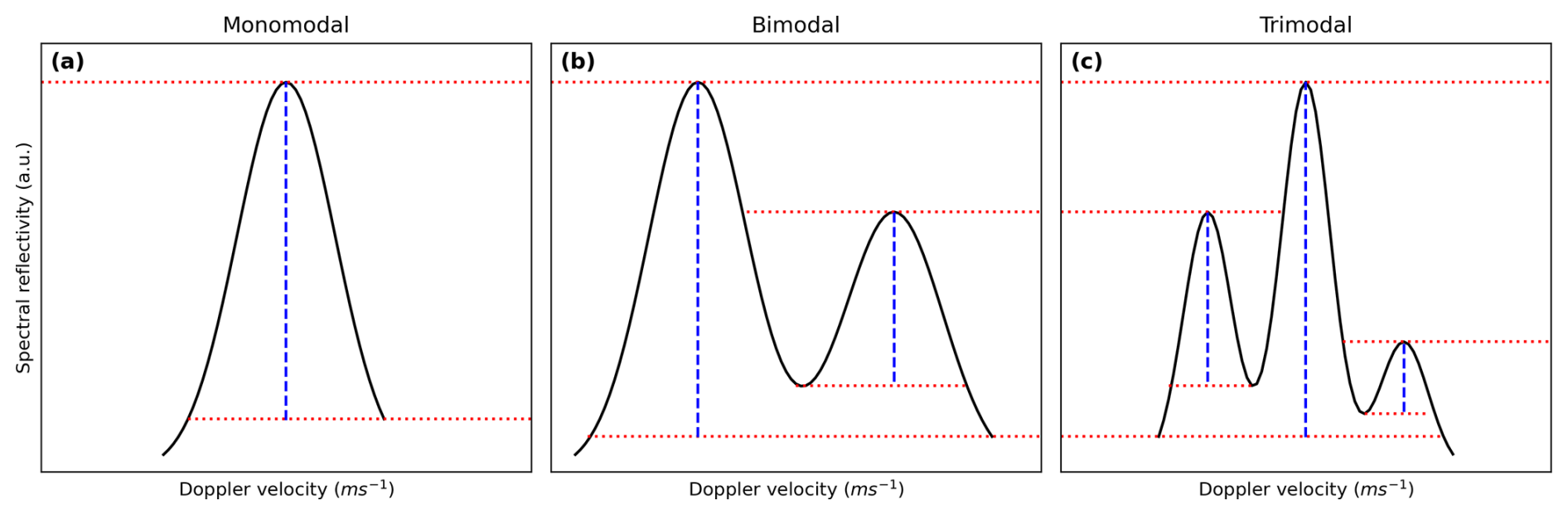
Figure 4 Idealised monomodal (a), bimodal (b), and trimodal (c) spectra. The red dotted lines show the identified minima and maxima of the spectra, and the blue dashed lines show the difference between these; this equates to the prominence. See text for a more comprehensive description. The y axis shows spectral reflectivity in arbitrary units (a.u.) and the x axis represents Doppler velocity.

We remove peaks where the spectral reflectivity is more than 30 dB lower than the spectral reflectivity of the largest peak. This has little impact on the overall results, but helps remove artefacts identified on the very edge of the one dimensional spectra which arise from imperfections in radar hardware. There are several other optional parameters which are described briefly in Table 3, but we found no significant change in results when they were applied and were therefore not implemented for simplicity.

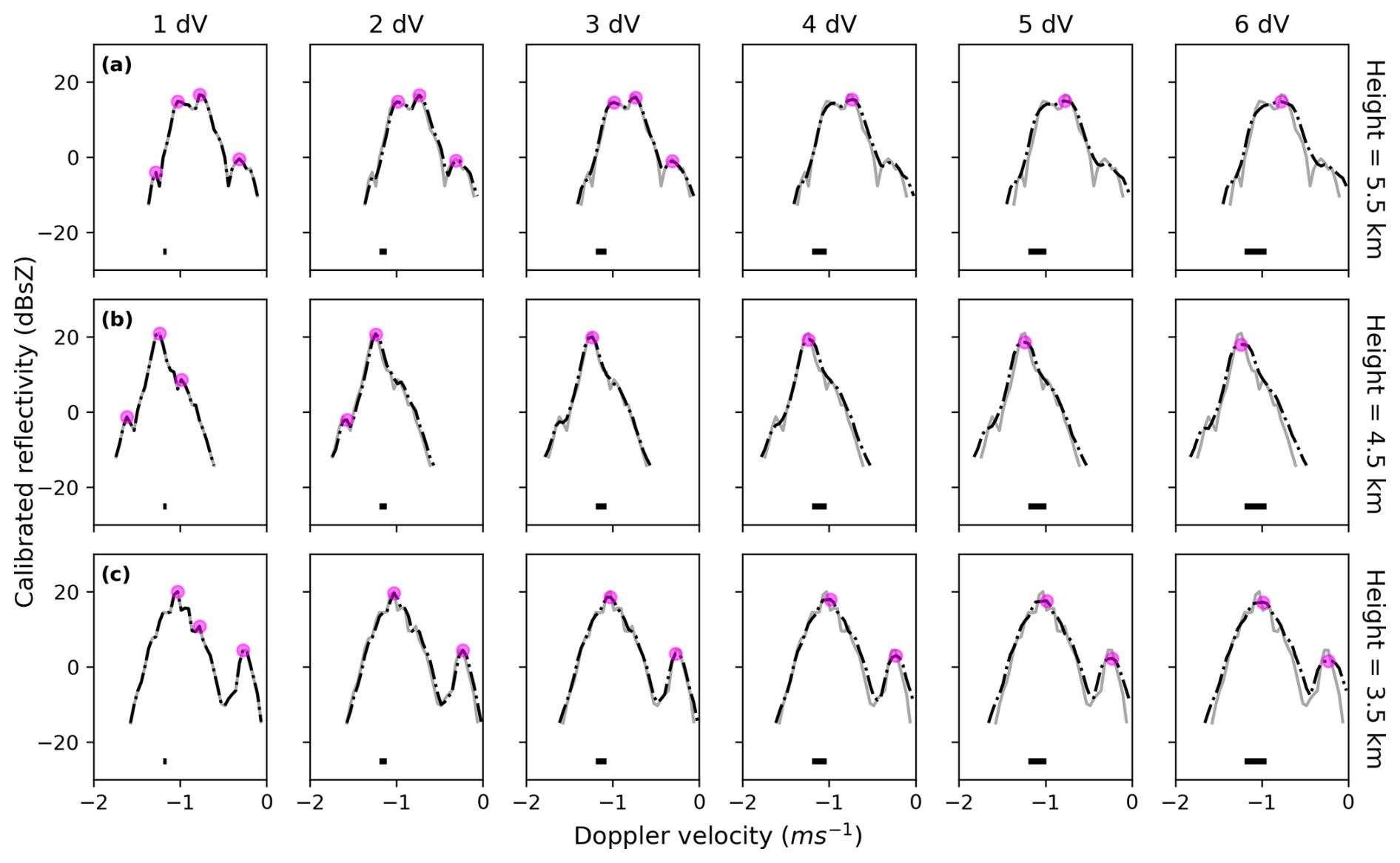
Figure 5 One dimensional Doppler spectra from heights of 5.5 km (a), 4.5 km (b) and 3.5 km (c) from the example shown in Fig. 1. The grey line in each panel shows the spectra with no smoothing, and the black line shows the smoothed spectra calculated using increasing averaging windows. The length of the averaging window is described by the number of velocity bins that the moving average is calculated across; dV is the velocity bin width, equal to 0.042 m s⁻¹. Note that the grey line is not visible when the averaging window is 1 dV as this equates to no smoothing. The thick black line at the bottom of each panel represents the width of the averaging window relative to the velocity scale. The peaks identified by the peak finding algorithm using the parameters described in Table 3 for each spectra are shown by the magenta points.

The one dimensional Doppler spectra for each pixel are noisy in their raw form due to the influence of receiver noise, and because weather echoes fluctuate randomly as a result of the time-varying relative positions (and therefore relative phases) of the scatters (e.g. Keat et al., 2016), which manifests itself in random fluctuations in the value of the spectral reflectivity in each velocity bin. A moving average is therefore calculated for each spectra before the peak finding algorithm is applied. This prevents random variations in the spectral reflectivity profile being identified as peaks. Choosing the number of velocity bins (dV, each of width 0.042 m s⁻¹) to apply the moving average across is non-trivial; too short a window means not enough of the noise is smoothed out, whilst too long a window causes the peaks to lose magnitude and separation, and they therefore begin to merge into each other. It is also important to inspect whether the chosen averaging window works equally well on monomodal and multimodal spectra, as well as in cases where the velocity separation between coexisting populations is marginal. Figure 5 shows examples of the process by which this parameter was chosen. With the prominence threshold fixed at 1 dB, we increase the averaging window gradually and apply the peak finding algorithm to each smoothed spectra to show when the “true” peaks are being correctly identified without noise contamination, and when peaks start to be lost due to over-smoothing – this occurs when the prominence of a peak falls below the 1 dB threshold. Figure 5a shows an example of a marginal multimodal spectrum, where small changes in the peak finding methodology have the most influence over the classification of this spectrum. We see that an averaging window of at least two velocity bins is required to smooth the noise; this prevents identification of the narrow peak on the left tail of the distribution, which is unlikely to be caused by microphysical features. However, we see in this example that a small change in the averaging window of three to four velocity bins would make the difference between spectra like these being identified as trimodal or monomodal. Comparison with the full Doppler spectrogram shown in Fig. 1 provides insight into the microphysical properties at this height, and we see that it is likely that there are multiple collocated particle populations. Figure 5b shows an example of a monomodal spectrum, where we would expect only one particle population to be identified. The importance of choosing the correct averaging window is again apparent in this example, as it is clear that the noisy nature of the raw spectrum has a greater influence. Here, an averaging window of at least three velocity bins is required to effectively smooth out the noise. Figure 5c shows a bimodal spectrum of two particle populations with very distinct vertical velocities. We expect that cases such as these should be comparatively easy for the algorithm to accurately detect the peaks. Indeed it can be seen that the “true” peaks are correctly identified with only a minimal averaging window of two velocity bins, and longer averaging windows do not change the results here. Taking these and many similar examples into account, we decide that an appropriate averaging window is three velocity bins (3 dV). This provides a good compromise between sufficient smoothing to reduce the impact of noise without reducing the signal of marginally differing populations in multimodal spectra. Once the peak finding algorithm has been applied to the individual smoothed Doppler spectra, it is useful to assess the temporal consistency of the number of identified peaks; this step is explained in the following section (Sect. 3.1.2). It is important to note that the averaging window needs to be worked out individually for different radars and calibrations.

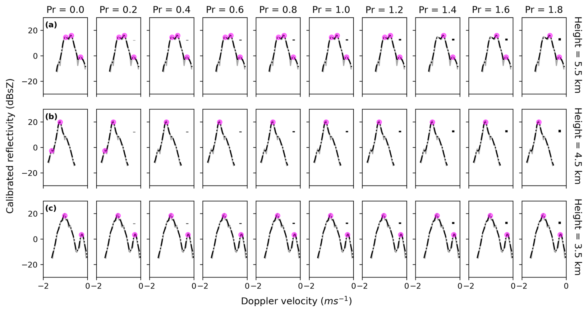
Figure 6 As Fig. 5, but showing the effect of changing the prominence (Pr in dB units) parameter. The window length for the moving average is fixed at three velocity bins. The one dimensional Doppler spectra are at heights of 5.5 km (a), 4.5 km (b) and 3.5 km (c) from the example shown in Fig. 1. The prominence value is varied and displayed above each column (see text and Table 3 for description). The thick black line in the top right corner of each panel shows the scale of the prominence thresholds relative to the spectra.

A similar test can be performed to show the effect of varying the value of the prominence threshold whilst fixing the averaging window at three velocity bins, the results of which are presented in Fig. 6. We find the small changes of this prominence threshold have less of an influence on the results than changing the averaging window length. In row (a), we see that the prominence threshold must reach 1.4 dB before it starts to influence the number of peaks identified for this spectrum. We find in row (b) that a low threshold of less than 0.4 dB causes an extra peak to be identified here. Inspection of the spectrogram shown in Fig. 1 suggests that the particle population at this height is monomodal, so we would expect a single peak to be identified here. This suggests that the low reflectivity peak identified in these spectrum is a result of noise in the observed Doppler spectrum which the averaging process has not smoothed completely. Figure 6 shows that even a relatively low prominence threshold is sufficient to remove features such as this, which demonstrates the importance of utilising this parameter. Row (c) shows that the prominence values tested here have no influence on the number of peaks detected for multimodal particle populations with peaks that are well separated in velocity and spectral reflectivity. Taking these and many such examples into account, we decide that a prominence threshold of 1 dB is sufficient to prevent “false” peaks being identified, but is not high enough to prevent the detection of particle populations separated by small changes in velocity and spectral reflectivity. Having settled on the value of the prominence threshold independently, we find that it is in good agreement with the value used in previous studies which use machine learning techniques to identify peaks in one dimensional Doppler spectra (Radenz et al., 2019; Vogl et al., 2024).

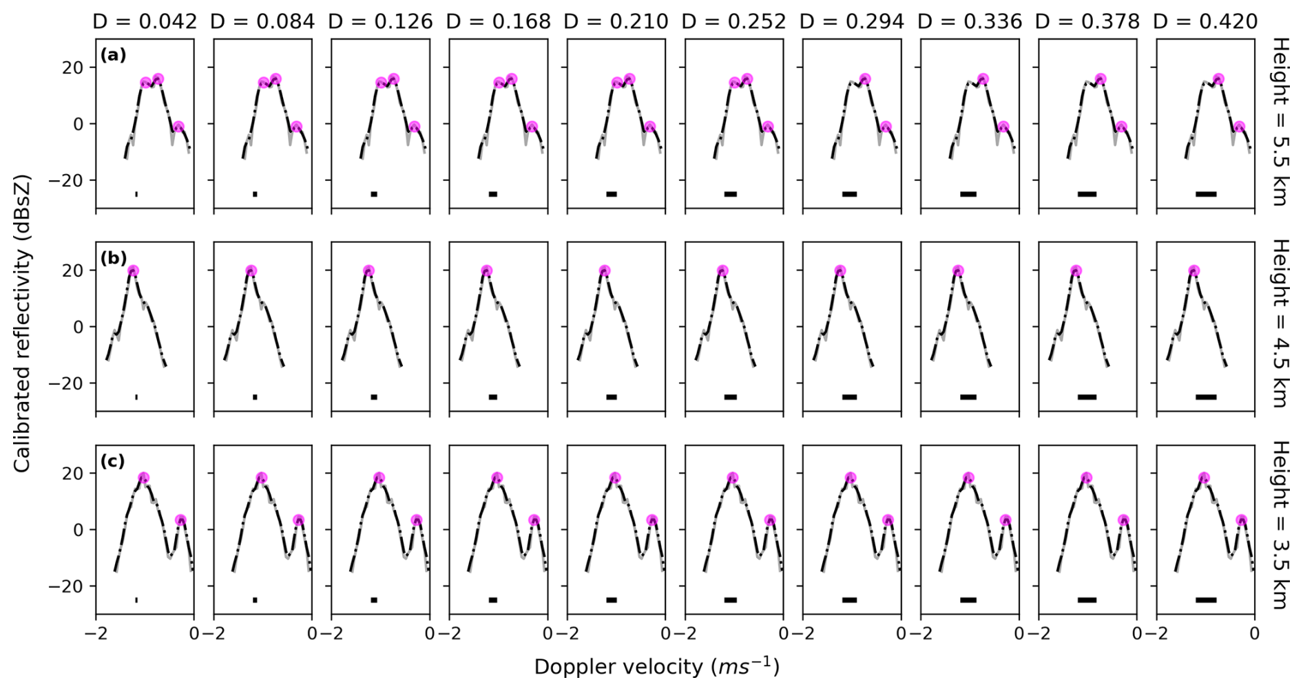
Figure 7 As Fig. 5, but showing the effect of changing the distance (D in m s⁻¹) parameter. The window length for the moving average is fixed at three velocity bins and prominence is fixed at 1 dB. The one dimensional Doppler spectra are at heights of 5.5 km (a), 4.5 km (b) and 3.5 km (c) from the example shown in Fig. 1. The distance parameter is varied and displayed above each column (see Table 3 for description); these values equate to a range of 1–10 velocity bins. The thick black line at the bottom of each panel shows the scale of the distance parameter relative to the spectra.

The distance parameter describes the minimum distance from the main peak that subsequent peaks can be identified. Figure 7 demonstrates the effect of changing this parameter on the number of peaks identified. Here, the averaging window was fixed at three velocity bins and the prominence threshold was held at 1 dB. Row (a) shows that the distance parameter must be increased to at least seven velocity bins (0.294 m s⁻¹) to influence the number of peaks detected in this spectrum. However, it seems likely that each of the three peaks identified when the distance parameter is removed are caused by genuine microphysical variations in this cloud volume, and it is therefore undesirable to limit the number of these peaks which are identified. Monomodal populations are inherently unaffected by the implementation of the distance parameter, as demonstrated in row (b). Multimodal populations with large separations between the identified peaks are similarly unaffected by the distance parameter. Based on this and many similar tests, we decided not to utilise the distance parameter as it risked causing peaks in the reflectivity spectrum caused by true microphysical variation to be ignored, whilst having little to no impact on the vast majority of spectra.

Whilst this peak finding method is accurate in ice and mixed phase cloud regions, it has not been tested in liquid phase regions. However, we find that it is inaccurate in rain because it has a broad and noisy reflectivity spectrum. For this study, we are interested in processes active in ice and mixed phase regions of cloud, and therefore apply a temperature threshold to neglect spectra at temperatures warmer than 0 °C.

3.1.2 Validating peak finding parameters

To confirm that the peak finding algorithm is working accurately, we examine the number of peaks identified per pixel against a spectrogram. An example of the results from this comparison are shown in Fig. 8. Panel (a) shows the number of peaks detected at each range gate, panel (b) shows the modal number of peaks for that profile and panel (c) shows the identified peaks marked on the main spectrogram by the black points. The grey shading shows where the turbulence threshold has been exceeded (described in Sect. 2.1.2); it is possible to see that these shaded areas correspond to narrow bands of the spectrogram which appear to have been smudged and, in the case of the example at 3.6 km, have lost the distinction between the two particle populations. We find from panel (a) that generally the algorithm can correctly identify the difference between monomodal and multimodal spectra, but the exact number of peaks detected is a little noisy. We therefore assess for spatial and temporal continuity by calculating the modal number of peaks in a vertical span of 240 m (four range bins) and temporal span of 10 min (10 individual spectra). The dimensions for this modal window were varied to test whether the results change with a change in these dimensions. We found that using a window that included half or double the amount of pixels had very little impact on the results presented later (not shown for brevity); this gave us confidence that the peak finding results are not highly sensitive to the exact figures chosen here. Panel (b) shows that the modal number of peaks for this spectrogram is significantly more consistent with height compared to the raw results in panel (a). The modal number of peaks indicates multimodality at 3–4 and 5.5–6 km, which appears well correlated with the areas on the spectra in panel (c) in which multiple particle populations are visible. From 4–5.5 km, the modal number of peaks is consistently representative of a monomodal population, which is supported by the narrow width of the spectrogram shown in panel (c) in the same region. The location of the peaks on the main spectrogram in panel (c) support the argument that the algorithm is working accurately because we see that the identified peaks are aligned with the peaks in spectral reflectivity that are determinable by eye.

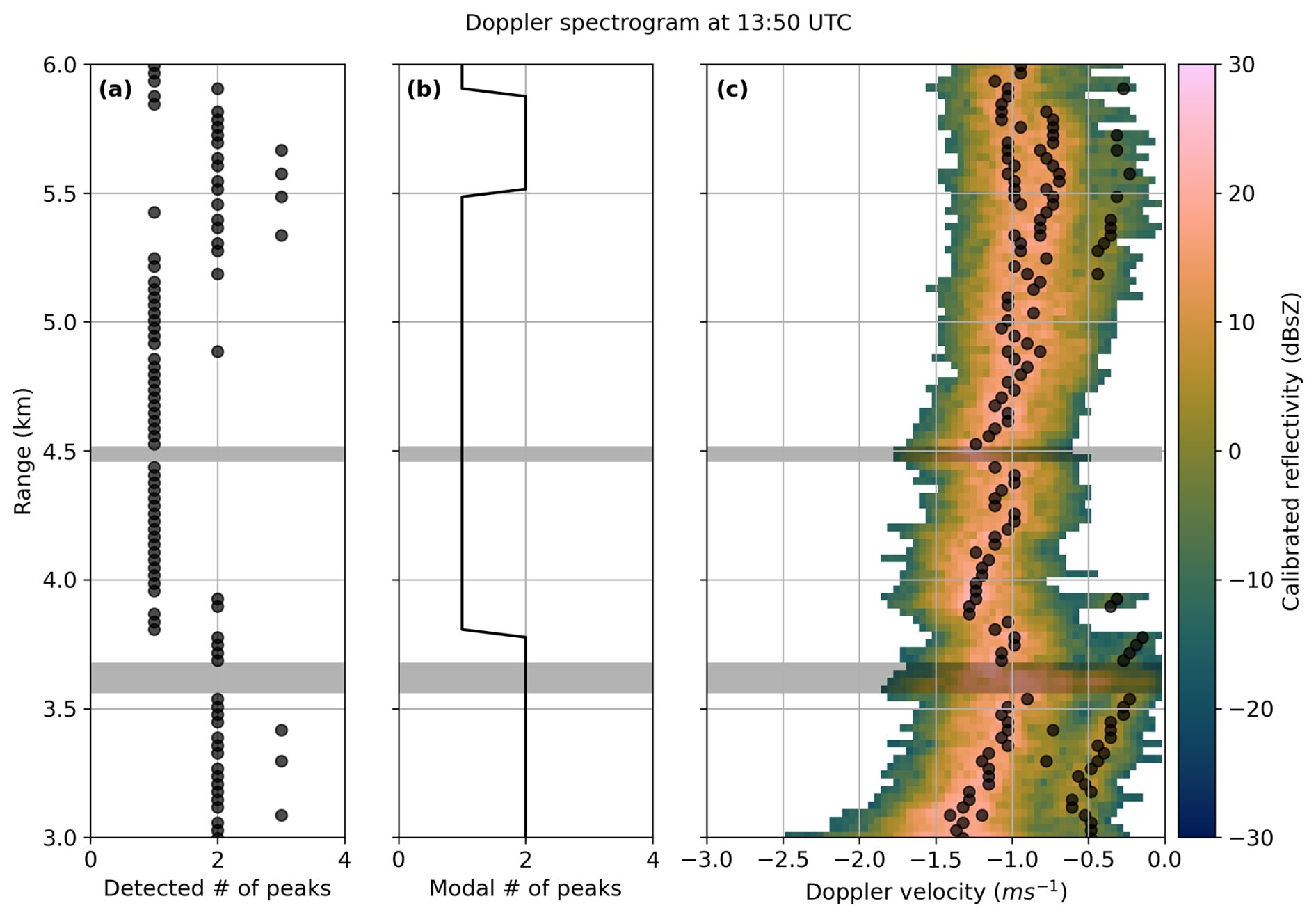
Figure 8 The number of peaks identified in each range gate is shown in panel (a), the modal number of peaks in a 240 m and 10 min window in panel (b), and the location of identified peaks on the main spectrogram of the example described in Sect. 2.1.1 is shown in panel (c). The grey shading in each panel shows where the turbulence threshold has been exceeded (see Sect. 2.1.2).

3.1.3 Separating particle modes

The peak finding method not only provides an estimate of the number of peaks identifiable in each spectrum, but also the velocity at which these peaks occur, from which the spectral reflectivity of these peaks is also discernible. This provides a wealth of information about the individual particle populations that would not be available from knowing solely the number of identified peaks per pixel. The primary population is identified based on the assumption that this population has the greatest spectral reflectivity, an approach also taken by Wugofski et al. (2025). We therefore assign any population at slower velocities than the primary population to the “slow mode” and any populations at faster velocities to the “fast mode”. Inspection of these identified “fast mode” populations suggests that they are data artefacts on the fringes of spectra resulting from imperfections in the analogue sampling of the in-phase and quadrature components of the radar signal. However, they are identified in only ∼ 2 % of spectra and are disregarded in the analysis that follows. Whilst this method generally provides an accurate estimate of the primary and secondary velocities, there are times when the diagnosis of primary and secondary peaks can be ambiguous. This happens when there are two populations with very similar spectral reflectivities, so that the spectral reflectivity of one population is not consistently bigger than the other. However, the proportion of these ambiguous cases is very small and affects isolated spectra, not whole cloud systems or cases. This occasional ambiguity therefore has a limited impact on the analysis that is performed using these results.

4 Results and Discussion

In this section, we present two case studies in detail, chosen to represent the variation observed among the selected case studies outlined in Table 2. We present standard moment level data for each case to help provide context, then show the results from our peak finding method described in Sect. 3.1. We qualitatively assess the findings from these two examples and discuss the mechanisms that may be responsible for the multimodal spectra observed in these cases. Results from the peak finding method for all cases described in Table 2 are shown in the Supplement. Using results from all cases, we then provide a quantitative estimate for the distribution of identified multimodal spectra with temperature. We analyse the peak velocities identified using the peak finding technique to investigate how the vertical velocity of particles varies between monomodal and multimodal regimes. This is then compared to the vertical distribution of MDV to assess the influence of multimodal particle populations on measurements of MDV. This has applications for interpretation of data from ground based instruments, but also for spaceborne Doppler radar such as that on the Earth Cloud, Aerosol and Radiation Explorer (EarthCARE) satellite (Illingworth et al., 2015; Wehr et al., 2023).

4.1 Case study: 6 January 2017

On 6 January 2017, an area of relatively deep low pressure, centred between Iceland and Scandinavia, was associated with a complex multi-fronted system. A warm front and two occluded fronts associated with this system passed over the UK before meeting a blocking high pressure centred over Central Europe. An ice cloud associated with these fronts was observed, which was up to 7 km deep above the melting layer (which remained at around 2 km throughout the day). Moment level observations of this cloud made by the Copernicus radar (described in Sect. 2.1) are shown in Fig. 9. Here we show the reflectivity in Fig. 9a, MDV in Fig. 9b, and spectral width in Fig. 9c. A thin layer of low level cloud is present for several hours during the first half of the day along with some upper level cirrus (see Fig. S1 in the Supplement), before the thick frontal cloud comes into the view of the radar at around 13:00 UTC and persists for the rest of the day. There are hints of microphysically interesting features in this cloud such as discernible regions of increased spectral width that correspond to “streaks” in the reflectivity and changes in MDV, for example between 14:00 and 17:00 UTC and between 21:30 and 23:30 UTC at heights of approximately 2–3 km. There was moderate rainfall associated with this cloud, shown in Fig. 9d, which started at 14:00 UTC and continued for the rest of the day, reaching peak values of ∼ 4 mm h⁻¹ between 23:00 and 00:00 UTC.

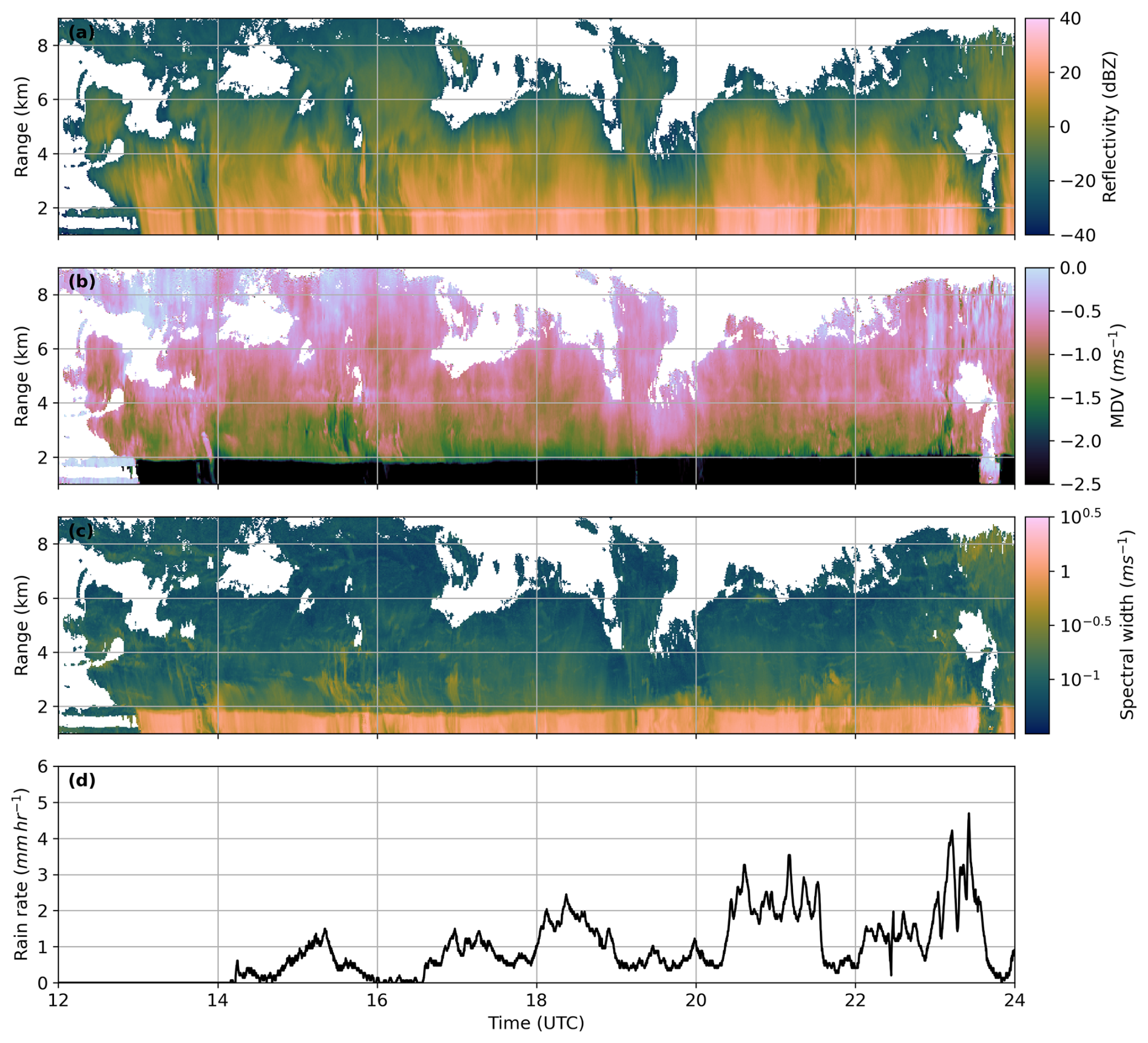
Figure 9 Moment level observations of reflectivity (a), mean Doppler velocity (b) and spectral width (c) from the Copernicus radar and rain rate (d) measured at CFARR for 6 January 2017.

Microphysical features, such as those mentioned above, can be investigated in greater detail using the results from the peak finding method described in Sect. 3.1. From this method we have an estimate of the number of peaks observed in the Doppler spectra for each pixel in a cloud, and the Doppler velocities for both the primary and secondary populations. The results from this analysis are shown in Fig. 10 and Fig. 11. Figure 10a shows the number of identified peaks per pixel and Fig. 10b shows the skewness of the Doppler spectra. It is useful to compare the location of identified multimodal spectra against the skewness of the one-dimensional Doppler spectra, as multimodal particle populations are thought to cause the shape of the Doppler spectra to deviate from that of a Gaussian distribution. However, two separate identical modes could also cause the skewness to be zero as the distribution would be symmetrical. Fig. 11a shows the velocity of the primary population, Fig. 11b shows secondary velocities, Fig. 11c shows tertiary velocities and Fig. 11d shows the difference between the primary and secondary velocities. Temperature contours from archived ICON data are shown in blue on all panels.

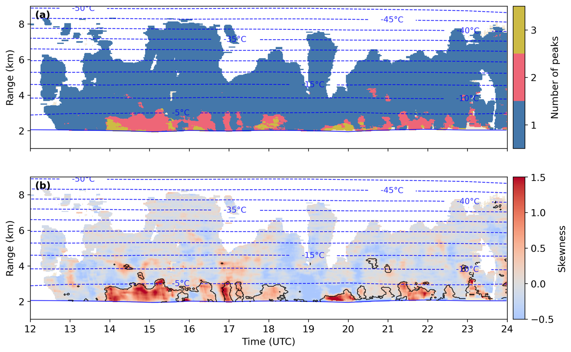
Figure 10 Number of peaks identified by the peak finding method (a) and skewness of the individual Doppler spectra (b) for 6 January 2017. The black contours in panel (b) show where multimodal spectra are detected. Blue contours show modelled temperature. The beige shading in panels (a) and (b) shows cloud pixels that were removed during filtering for turbulence and attenuation; this is only visible in very small patches in this cloud (for example 23:00 UTC at 2 km).

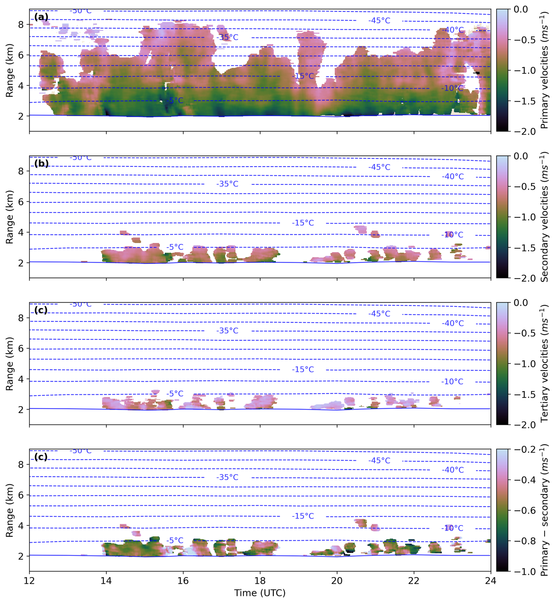
Figure 11 Primary mode velocities (a), secondary velocities (b) and tertiary velocities (c) for 6 January 2017. Panel (d) shows the difference between the primary and secondary velocities. Blue contours show modelled temperature. The beige shading in panel (a) shows cloud pixels that were removed during filtering for turbulence and attenuation. Note the change in colour scale in panel (d) where the difference is in the absolute sense, i.e. −1 m s⁻¹ is the greatest difference, −0.2 m s⁻¹ is the smallest difference.

We find that multimodal spectra are frequent between the temperatures of −5 and 0 °C from around 14:00 UTC until the end of the observed period. It is interesting that the number of peaks also increases with increasing temperature in some parts of this layer; there is a visible shift from bimodal to trimodal spectra with increasing temperature at 14:00–15:00, 17:30–18:30, and 19:00–20:00 UTC. Inspection of spectrograms at different times, for example those shown in Fig. 12, reveal that there were indeed a mixture of trimodal (Fig. 12a) and bimodal (Fig. 12b) spectra observed on this day. At temperatures between −5 and −15 °C, there are a handful of isolated regions with multimodal spectra at approximately 14:00–15:00 and 20:00–21:00 UTC. Multimodal spectra are almost non-existent at temperatures colder than −15 °C. Comparison with the skewness shown in Fig. 10b reveals that the location of multimodal spectra identified by the peak finding method is largely consistent with regions of positive skewness. Consistent with von Terzi et al. (2022), skewness appears to increase at temperatures colder than the multimodal spectra identified by the peak finding algorithm; this may suggest that skewness is sensitive to multimodal particle populations where the two populations are too similar to be separated by the peak finding algorithm. An understanding of the microphysical processes that are active in this case may be gained by examining the velocities in Fig. 11. We find at temperatures lower than −5 °C, primary velocities (Fig. 11a) remain consistent with height. At temperatures greater than −5 °C, we see that the primary velocity increases as particles fall, with velocities reaching −1.5 to −2 m s⁻¹. These increases in velocity are correlated with the presence of multimodal spectra. This suggests that the process responsible for producing multimodality in the Doppler spectra is connected to the increased primary mode vertical velocities. Riming causes increased particle fall speeds due to increased mass, without causing particles to grow much in size; this is because it acts to “fill in the gaps” of open structured particles such as dendrites and aggregates before adding to the overall size (e.g. Garrett and Yuter, 2014; Kneifel and Moisseev, 2020). Riming necessarily occurs in environments which are saturated with respect to liquid water, and therefore splinters which may be produced by rime splintering can rapidly undergo vapour growth to form needle and column crystals which fall at a distinctly slower speed than the rimed population. If they grow large or fast enough, the needle and column crystals themselves will begin to rime. Secondary and tertiary velocities (Fig. 11b and c) also appear to increase as temperature increases, suggesting particle growth, but interestingly the difference between the primary and secondary velocities (Fig. 11d) appears to remain relatively constant. Examination of the velocities shown on the spectrograms in Fig. 12 suggests that this may result from similar rates of increasing particle population velocities.

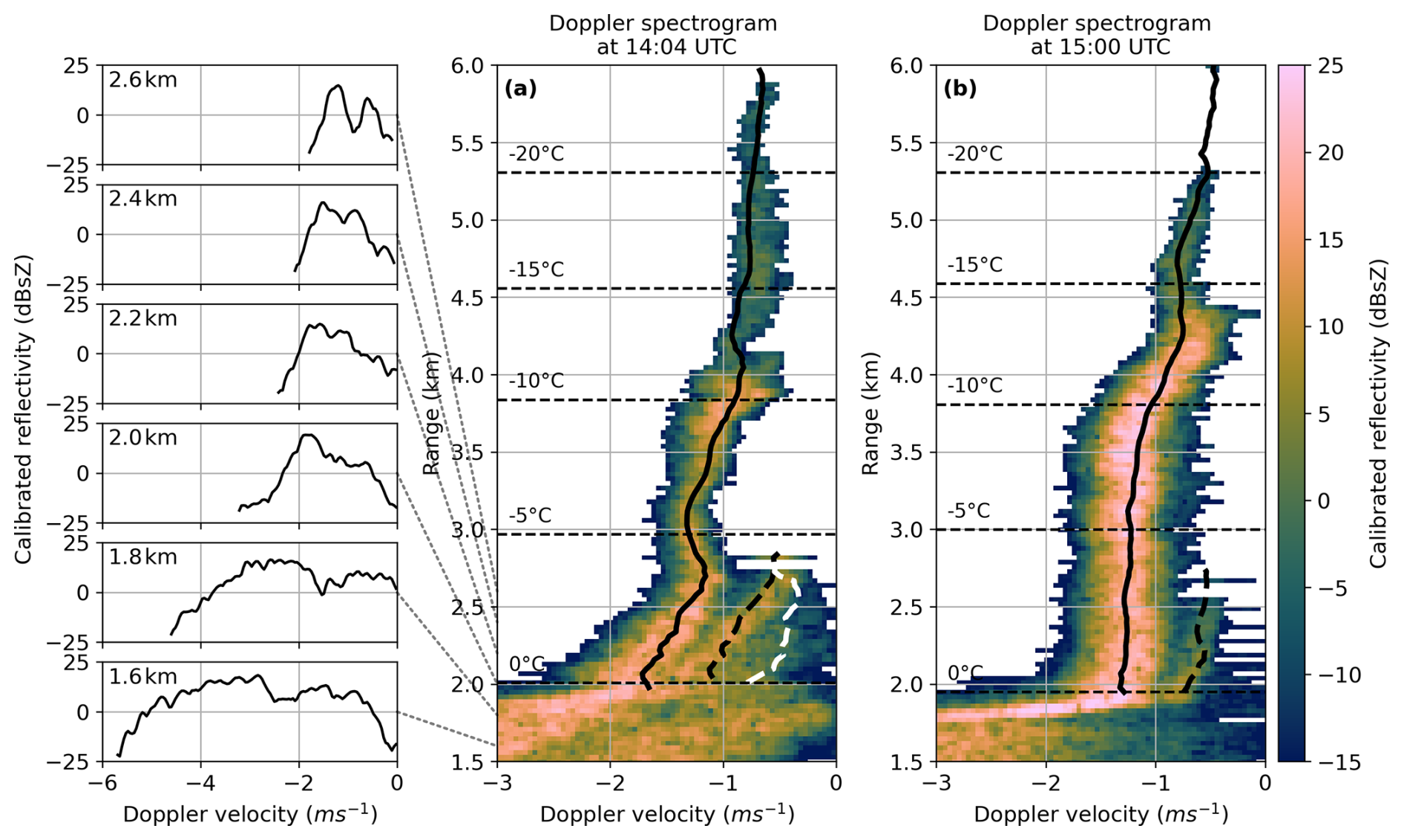
Figure 12 Examples of spectrograms with trimodal (a) and bimodal (b) signatures for 6 January 2017. Panel (a) includes one-dimensional Doppler spectra for a range of heights around the melting layer, and demonstrate that the drizzle mode remains visible in the liquid phase region of the spectrogram. The primary (solid line), secondary (black dashed line) and tertiary (white dashed line) velocities are also shown.

Example spectrograms shown in Fig. 12 support the suggestions outlined above. Figure 12a shows evidence that both a secondary ice mode and a drizzle mode are present at this time, which corresponds to a region where trimodal spectra were identified (shown in Fig 10a). The drizzle mode is first visible at 2.75 km, and is identifiable as the vertical velocity of the population does not rapidly increase at the melting layer, and indeed remains separate in the rain below. The one-dimensional Doppler spectra shown in Fig. 12 shows that the drizzle mode is visible as a tertiary peak in the Doppler spectra above the melting layer, and is also visible as a separate population below the melting layer. The velocity of the primary population increases rapidly at the same height as the drizzle mode is first visible, which suggests the primary population is riming. One explanation for the production of the secondary ice particle mode is therefore rime splintering; cloud droplets are required to form and grow drizzle drops, so the presence of drizzle shows that there is liquid water present at temperatures associated with rime splintering and that liquid water droplets are therefore available for riming. Another explanation is that droplet fragmentation is producing the secondary ice population here, as it is possible that some of the drizzle drops will freeze and produce secondary particles via the mechanisms described by Lauber et al. (2018). Figure 12b shows a secondary particle mode is visible at heights of approximately 2–2.5 km, which corresponds to temperatures of approximately −3 to 0 °C. This secondary mode consists of ice particles as it melts at 0 °C, as seen by the rapid increase in vertical velocity of the population. It seems unlikely that droplet fragmentation is producing the secondary mode here due to the lack of a drizzle mode in the Doppler spectrogram; it follows that rime splintering may be responsible but without knowledge of whether cloud droplets are present, it is not possible to definitively ascertain the mechanisms that may be active. The primary population velocity increases from the top of the profile to around −17 °C, where a slight decrease in velocity is apparent and reaches a minimum at approximately −13 °C. This feature has been observed previously (e.g. von Terzi et al., 2022), and the potential mechanisms responsible for producing this feature are discussed in greater detail in Sect. 4.4. Particle velocities gradually increase again from around −13 to 0 °C.

4.2 Case study: 17 May 2017

On 17 May 2017, low pressure conditions were dominant over the UK resulting in several frontal features which passed over the UK throughout the course of the day. Associated with these frontal features was a long-lived ice cloud which was up to 8 km deep above the melting layer and which persisted for the majority of the day. The melting layer was at about 3 km and dropped slightly in height throughout the day. Moment level observations of this cloud are shown in Fig. 13, with reflectivity in Fig. 13a, MDV in Fig. 13b and spectral width in Fig. 13c. At a glance, this appears to be a more homogenous cloud than that in the previous case study, with fewer clear microphysical features. There is a region at 5–6 km between 10:00 and 15:00 UTC with MDV that is lower than the surrounding regions, and the values of MDV observed here are less than −0.5 m s⁻¹. Interestingly, Fig. 15a shows that the velocities of the primary population also decrease in the same region. We see that there are increased values of spectral width at 13:00 UTC which correspond to a disturbance of the melting layer which is visible in Fig. 13a–b. Figure 13d shows the rain rate, which remains moderate to heavy throughout the day, with an intense shower at 13:00 UTC. This very heavy shower corresponds with the disturbance in the melting layer visible in Fig. 13a–c, which suggests that this feature is a cell of embedded convection. Figure 2 shows that the turbulent contribution to spectral width is high in this region, and is therefore removed when the turbulent filtering method described in Sect. 2.1.2 is applied.

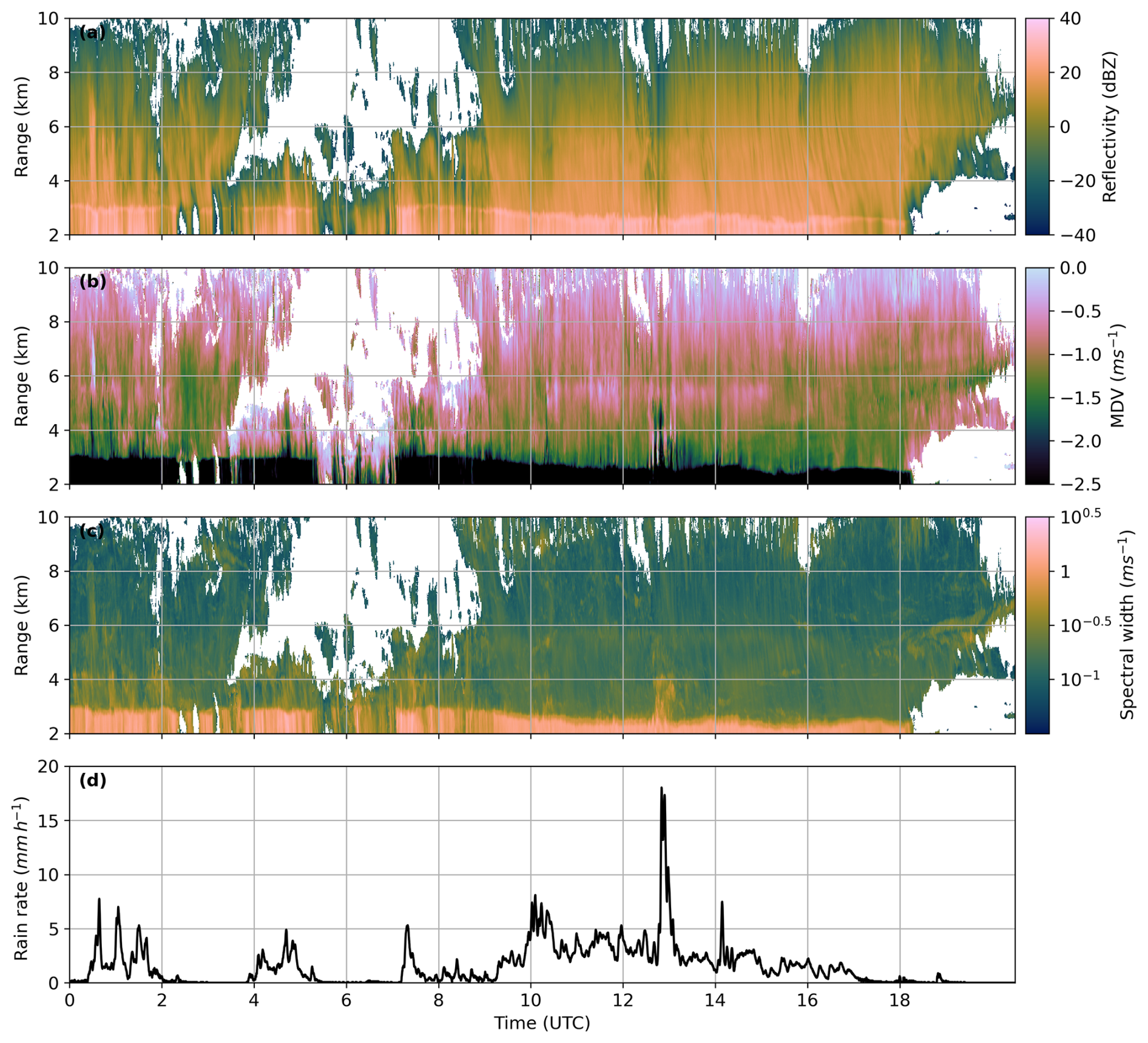
Figure 13 Moment level observations of reflectivity (a), mean Doppler velocity (b) and spectral width (c) from the Copernicus radar and rain rate (d) measured at CFARR for 17 May 2017.

The results from the peak finding method can again be used to infer what processes are influencing the development of this cloud, and are presented in Fig. 14. Figure 14a shows the number of identified peaks and Fig. 14b shows the skewness of the one-dimensional Doppler spectra. As described in Sect. 4.1, skewness is an indication of how much the one-dimensional Doppler spectra deviate from a symmetric distribution. We see that the regions of high skewness are largely consistent with regions of multimodality detected by the peak finding algorithm. We see that the distribution of multimodal spectra in this example is different to the that examined in Sect. 4.1. Almost all multimodal spectra are bimodal, expect a few isolated regions early in the observation period which are trimodal. From Fig. 14a, we can see that at temperatures between −5 and 0 °C, multimodal spectra are prevalent throughout much of the cloud. Figure 14 shows the velocities of the different populations in this cloud; Fig. 14a shows the velocity of the primary population, Fig. 14b shows the velocity of the slow mode and Fig. 14 shows the velocity difference between the two populations. Similarly to the case analysed in Sect. 4.1, we suggest that the multimodality observed is associated with riming, as there are increased primary velocities visible in Fig. 14a that are consistent with particles influenced by riming; particle velocities are approximately −1.5 m s⁻¹ throughout much of the cloud layer at temperatures between −5 and 0 °C. The slow mode velocities in this layer, shown in Fig. 14b, appear to increase with temperature. The difference in velocity between the two populations (Fig. 14c) decreases with increasing temperature, indicating growth of the secondary population. The presence of the slow particle mode, together with its increasing velocity with temperature, strengthens the argument that riming is active at these temperatures. Consequently, rime splintering may also be active and responsible for the presence of the slow particle mode. Given the lack of trimodal spectra in this case, it seems unlikely that fragmentation during freezing of drizzle drops is producing the observed multimodal signatures; spectrograms shown in Fig. 16 support this idea as there is no evidence of a drizzle mode. We also find that between temperatures of −10 and −15 °C there are frequent multimodal regions. The mechanism behind this multimodality is unclear, as this is outside the temperature range which is expected for the rime splintering mechanism. The velocity of the secondary population at these temperatures is very slow at around −0.25 m s⁻¹. As dendritic growth is preferential at these temperatures, it follows that the slow particle mode may consist of small plate-like or dendritic particles which fall slowly due to relatively large surface areas resulting in increased air resistance. It is also possible that small drizzle drops (∼ 100 µm) would produce a similar signature here, but it seems unlikely that they would persist at these temperatures in stratiform cloud.

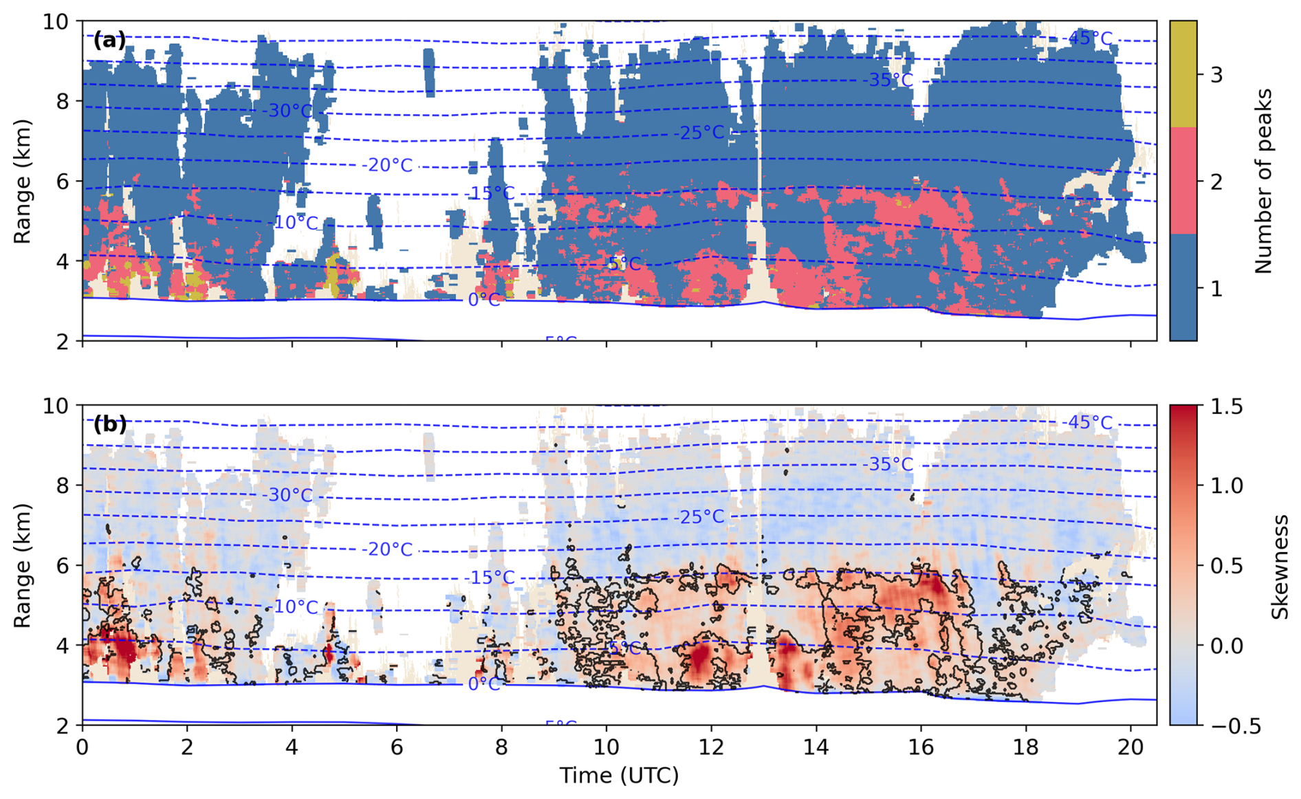
Figure 14 Number of peaks identified by the peak finding method (a) and skewness of the individual Doppler spectra (b) for 17 May 2017. Blue contours show modelled temperature. The black contours in panel (b) show where multimodal spectra are detected. The beige shading in panels (a) and (b) shows cloud pixels that were removed during filtering for turbulence and attenuation.

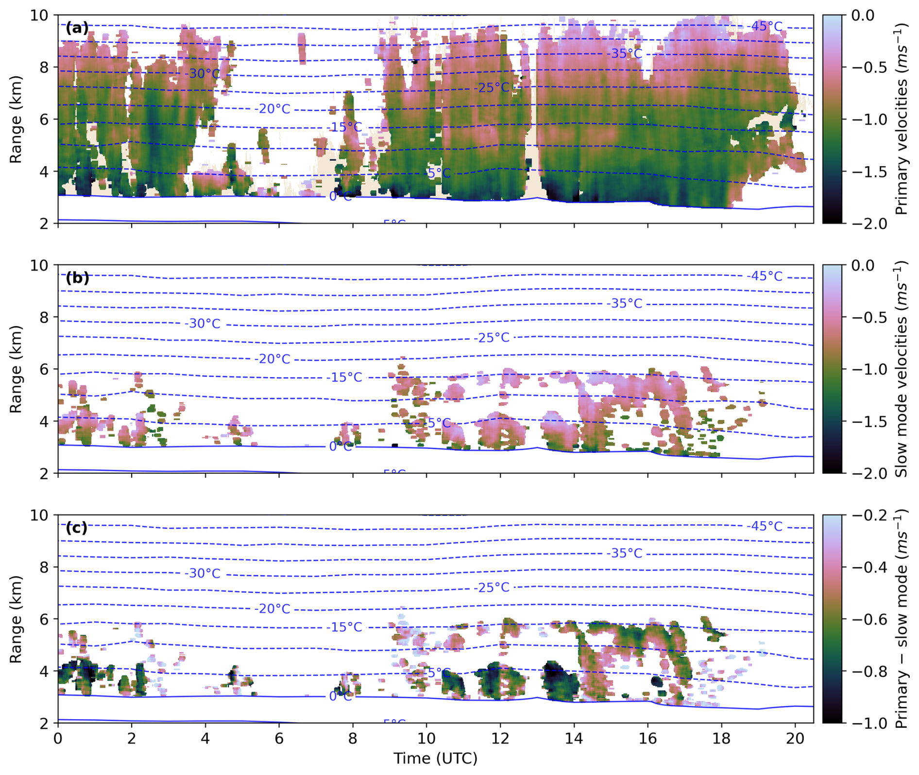
Figure 15 Primary mode velocities (a), slow mode velocities (b) and the difference between the primary and slow mode velocities (c) for 17 May 2017. Blue contours show modelled temperature. The beige shading in panel (a) shows cloud pixels that were removed during filtering for turbulence and attenuation. Note the change in colour scale in panel (c) where the difference is in the absolute sense, i.e. −1 m s⁻¹ is the greatest difference, −0.2 m s⁻¹ is the smallest difference.

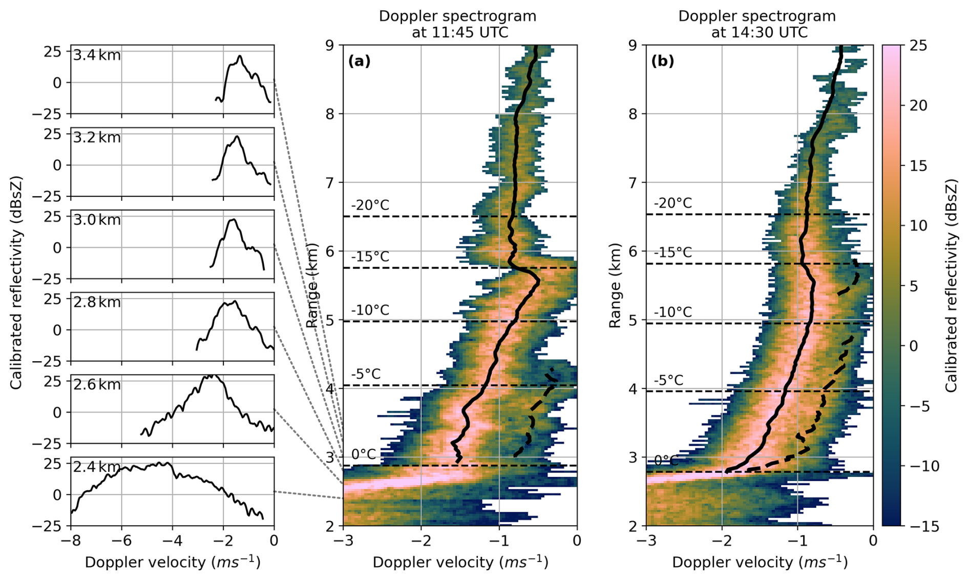
Figure 16 Examples of spectrograms with bimodal signatures at −5 °C (a) and both −5 and −15 °C (b) for 17 May 2017. Panel (a) includes one-dimensional Doppler spectra for a range of heights around the melting layer, and demonstrate that the secondary mode consists of ice as it does not retain a separate peak in the liquid phase region of the spectrogram. The primary (solid line) and secondary (dashed line) velocities are also shown.

Figure 16 shows two examples of spectrograms observed during this case study. In Fig. 16a, a secondary population is visible that forms at approximately −7 °C and increases in vertical velocity, but remains distinct from the primary population. In Fig. 16b, it is possible to see a secondary population which forms at −15 °C and grows until the velocity becomes indistinguishable from the primary population at approximately −10 °C. Another secondary population is visible from around −7 °C to the melting layer. It is clear that the secondary populations shown in Fig. 16a and b are ice as they rapidly increase in velocity at the melting layer, thus suggesting that drizzle is not prevalent in this case; one-dimensional spectrograms shown support this suggestion as there is only population visible below the melting layer.

4.3 Statistics from all case studies

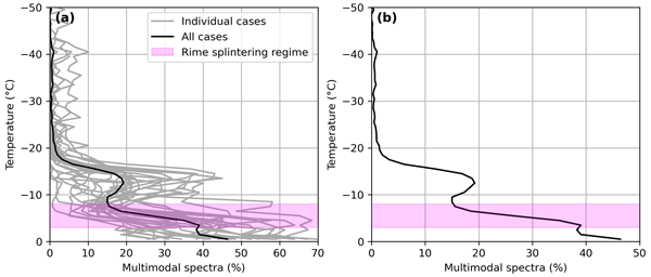
In Sect. 4.1 and 4.2, we have qualitatively analysed the distribution of multimodal spectra with temperature, and discussed possible mechanisms influencing the development of the clouds in these case studies. In order to make these findings applicable more generally, it is useful to quantify the distribution of multimodal spectra with temperature across all of the case studies outlined in Table 2. We therefore calculate an estimate of the fraction of “in-cloud” pixels where multimodal spectra are observed and the results of this analysis are shown in Fig. 17. The grey lines show the results for individual case studies, and the black line shows the overall statistics. Wugofski and Kumjian (2025) show statistics of multimodal spectra identified using moment-level variables but to the best of our knowledge, the frequency of observed multimodal spectra identified by analysis of spectral reflectivity has not been quantified in this way previously.

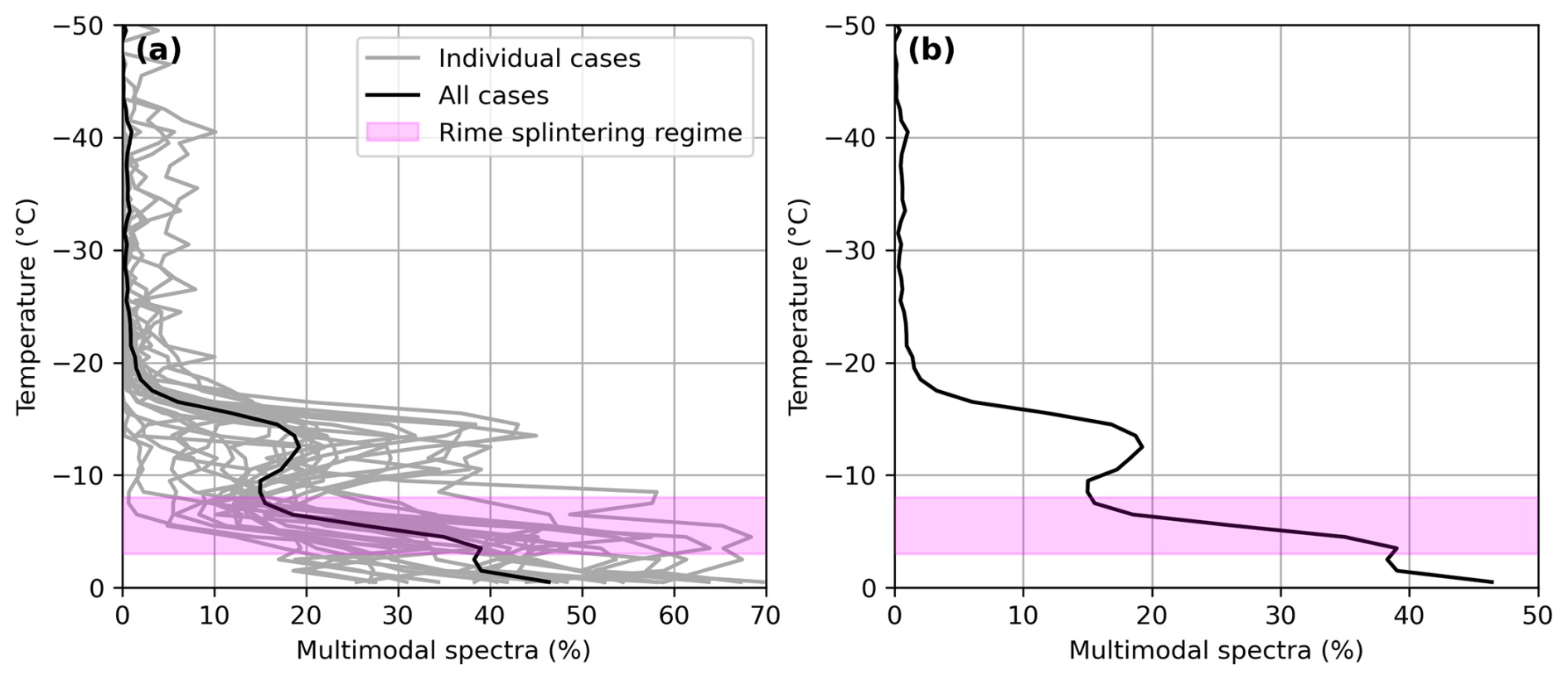
Figure 17 Percentage of “in-cloud” pixels with observed multimodal spectra. (a) The grey lines show the results for individual cases, and the black line shows the statistics across all case studies. (b) The distribution from all case studies is shown individually for clarity. The rime splintering regime is shown in magenta (based purely on temperature). Note the different x-axis limits between panels.

The magenta shading in this figure highlights temperatures from −3 to −8 °C, which is the temperature range in which it is thought that the rime splintering mechanism is active (Field et al., 2017; Korolev and Leisner, 2020, and references therein), and indeed previous studies have shown in situ observations of particles which are consistent with rime splintering being observed at these temperatures (e.g. Crosier et al., 2011, 2014; Keppas et al., 2017; Mammatt et al., 2026). However, as the mechanism behind rime splintering remains uncertain, references to the “rime splintering regime” throughout this section are referring the range of the temperatures between −8 to −3 °C and are not intended to imply that rime splintering is necessarily active. We see that throughout this temperature regime, the percentage of multimodal spectra increases rapidly from approximately 15 % at −8 °C to 40 % at −3 °C. The percentage of multimodal spectra continues to increase at temperatures higher than this ice multiplication regime, which suggests that secondary particle populations continue to grow and evolve throughout this relatively narrow temperature band before reaching the melting layer. Individual cases vary in the magnitude of the percentage of multimodal spectra throughout this regime, but all follow broadly the same pattern.

At temperatures of −10 to −18 °C, we see an increase in the percentage of multimodal spectra from less than 5 % at −18 °C to a maximum of 20 % at −13 °C. This is outside of the temperature range that the rime splintering mechanism is thought to be active in, so we expect that a different mechanism is causing the observed multimodality. It is possible that new particles at these temperatures are formed by primary nucleation and that the newly-formed dendritic particles fall slower than crystals falling from above, leading to two populations of ice crystals with distinctly different fall speeds existing in the same radar volume (e.g. Yan et al., 2025). This raises the question of why primary nucleation would consistently occur in this region. There is a lack of evidence in the current literature that ice nucleating particle (INP) concentrations increase at these temperatures, and instead observations support that idea that INP concentrations decrease with increasing temperature (e.g. DeMott et al., 2010). There have been studies which show that conditions here are potentially favourable for SIP; droplet fragmentation and ice-ice collisional fragmentation have been suggested as potential mechanisms for the production of secondary ice particles at temperatures outside the rime splintering regime (Field et al., 2017; Korolev and Leisner, 2020). Droplet fragmentation has received some attention in recent years (Phillips et al., 2018; Keinert et al., 2020; Lauber et al., 2021), and occurs when a drizzle drop spontaneously freezes and projects splinters as a result of a shattering ice shell. This process is unlikely to be the primary cause of multimodality observed at these temperatures, as we have not seen signatures consistent with a drizzle mode visible in the Doppler spectra at these temperatures. Trimodal spectra, which are likely to indicate the presence of a drizzle mode (see Fig. 12a), are only detected at temperatures warmer than −5 °C in Fig. 10a and there are very few trimodal spectra in Fig. 14a. Ice-ice collisional breakup has also been proposed as an efficient SIP mechanism (Vardiman, 1978; Yano and Phillips, 2011; Yano et al., 2016; Phillips et al., 2017), in which ice fragments are produced during collisions between ice particles. von Terzi et al. (2022) suggest a link between increased aggregation between dendritic particles and potential production of ice fragments formed during collisions. Dendritic growth on particles precipitating from above produces fragile branches which may be susceptible to fragmentation, and the fragments produced may have the potential to grow into a secondary particle mode. Whilst there have been laboratory studies carried out previously to investigate these processes, a lack of observational in situ evidence means uncertainty surrounding the efficiency and feasibility of these mechanisms remains high.

Multimodal spectra are very rare at temperatures lower than −20 °C, with just 0.64 % of all spectra at temperatures less than −20 °C identified as multimodal; this is in agreement with previous studies which support the argument that SIP is very inefficient at low temperatures (Field et al., 2017; Korolev and Leisner, 2020). However, Korolev et al. (2022) presented a case study of a precipitating cirrocumulus-nimbostratus cloud system with generating cells of turbulence, and suggested that SIP can be observed at temperatures as low as −27 °C. This demonstrates the continued importance of investigation into SIP processes active outside of the rime splintering regime.

4.4 Vertical profiles of peak velocities and MDV

The velocities associated with the peaks identified by the peak finding algorithm can help us gain understanding into how these vary with height; these velocities will be referred to as peak velocities throughout this section, as they are the velocity at which the peak spectral reflectivity is observed. Note that these are not MDVs for each population, but specifically the velocity at which the peak spectral reflectivity occurs. It is possible to separate the peak velocities into the different populations they represent, as described in Sect. 3.1.3, and in Fig. 18 we therefore show histograms of all peak velocities (a), all primary peak velocities (b), primary peak velocities from monomodal spectra (c), primary peak velocities from multimodal spectra (d) and slow mode velocities (e) against temperature. The medians from Fig. 18a–e are shown in Fig. 18f to facilitate simple comparison. This analysis shows some interesting features. We see from Fig. 18a–c that the vertical profile of all peak velocities, all primary peak velocities and monomodal primary velocities is generally similar, and Fig. 18f shows that the medians are frequently indistinguishable from each other. This suggests that the influence of secondary peaks on the overall distribution of velocities (Fig. 18a) is modest, but there are differences which demonstrate that this cannot be neglected. Here, we see that velocities in Fig. 18a–c increase with temperature from −50 °C, where the median velocity is approximately −0.6 m s⁻¹, to −18 °C, where the median velocity is around −0.9 m s⁻¹. There is a clear decrease in velocity between −18 and −13 °C, where the median velocity falls to around −0.8 m s⁻¹. Whilst this appears to be a small change, this equates to an 11 % reduction between the velocity at −18 and at −13 °C. We attribute this feature to dendritic growth on particles precipitating from above – that is, the growth of dendritic branches on polycrystals and aggregates formed at lower temperatures. These geometrically open dendritic features experience greater drag force than other crystal growth habits, and therefore fall more slowly for a projected area to given mass ratio (Heymsfield and Westbrook, 2010). From this velocity minimum at −13 °C, the median velocity increases with temperature for the rest of the profile, however the temperature range between −10 and 0 °C is where we see the greatest differences between these profiles. Figure 18a shows that the median velocity remains approximately constant at −1.1 m s⁻¹ between −8 and −3 °C, before increasing to −1.5 m s⁻¹ at 0 °C. In contrast, the median velocity in Fig. 18b increases mostly consistently from −1.0 m s⁻¹ at −10 °C to −1.3 m s⁻¹ at 0 °C. In Fig. 18c, we find that the median velocity increases gradually from −1.0 m s⁻¹ at −10 °C to −1.2 m s⁻¹ at 0 °C.

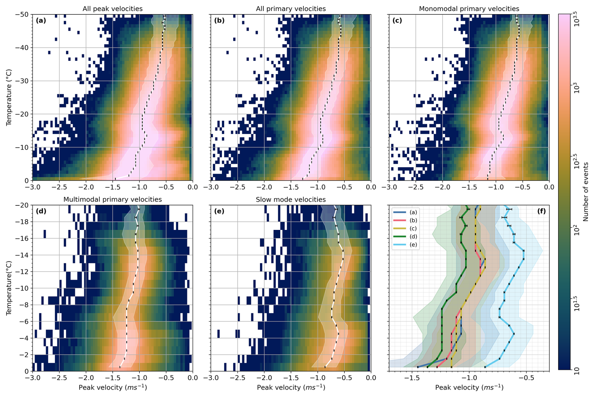
Figure 18 Vertical profiles of particle population velocities as 2D histograms. The white solid line shows the median and the white shading shows interquartile range in panels (a)–(e). Shown are all peak velocities (a), all primary peak velocities (b), primary peak velocities from monomodal spectra (c), primary peak velocities from multimodal spectra (d) and slow mode velocities (e). The medians and interquartile ranges of all distributions are shown in panel (f). The standard mean error, calculated as the width of the interquartile range divided by the square of the number of samples, is shown by the black bars. Note the logarithmic colour scale, change in y-axis limits between the top and bottom row and change in x-axis limits in panel (f).

Figure 18d–e show velocities associated with multimodal spectra. It is clear from Fig. 18f that the primary velocity from multimodal spectra is consistently higher than from monomodal spectra, remaining higher than −1 m s⁻¹ between temperatures of −20 and −10 °C, and increasing to approximately −1.3 m s⁻¹ throughout the rime splintering regime. This may suggest that riming is influencing the velocity of particles in this temperature regime, although the median velocity remains lower than −1.5 m s⁻¹; this is the threshold at which Kneifel and Moisseev (2020) suggest high vertical velocities can be reliably assigned to riming. Figure 18e shows the velocities of the slow particle mode, and demonstrates clearly the temperatures at which the slow mode is first detectable. The median velocity clearly shows the formation and growth of an appreciable slow falling population from −15 °C, where the median velocity is −0.5 m s⁻¹, to −10 °C, where the median velocity has increased to −0.7 m s⁻¹. Another growth regime is then visible from −5 °C, where the median velocity is −0.6 m s⁻¹, to 0 °C, where the velocity has increased to −0.8 m s⁻¹. This supports our argument for the existence of multiple populations at these temperatures, with the slow particle mode increasing in velocity as temperature increases suggesting growing particle size.

It is also possible to calculate the distribution with temperature of MDV; Fig. 19 shows this distribution for all spectra (a), monomodal spectra (b) and multimodal spectra (c). Figure 19d shows the medians from Fig. 19a–c for simpler comparison. We see from Fig. 19a–b that the profile of MDV with temperature is very similar in shape, but the median MDV from monomodal spectra is consistently slightly slower than from all spectra at temperatures higher than −15 °C. This is particularly visible in the lowest section of the profile between −5 and 0 °C (see Fig. 19d). Comparison with Fig. 18a and c shows that these profiles are consistent with the profiles of primary velocities from all spectra and monomodal spectra respectively. Interestingly, we see in Fig. 19c–d that the median MDV from multimodal spectra is consistently faster than from monomodal spectra throughout the whole profile, which is in agreement with the increased primary population velocities seen in Fig. 18d. This further supports the suggestion that the mechanism responsible for producing multimodal spectra acts to increase the velocity of the primary population, and that this has a greater influence on the MDV in both of the identified temperature regimes than the presence of the slow particle mode. However, monomodal spectra have a greater influence on the overall MDV at this temperature, as seen by the decreased MDV at −13 °C visible in Fig. 19a. Figure 17 shows that around 20 % of spectra are multimodal at this temperature, and therefore the majority of spectra are monomodal.

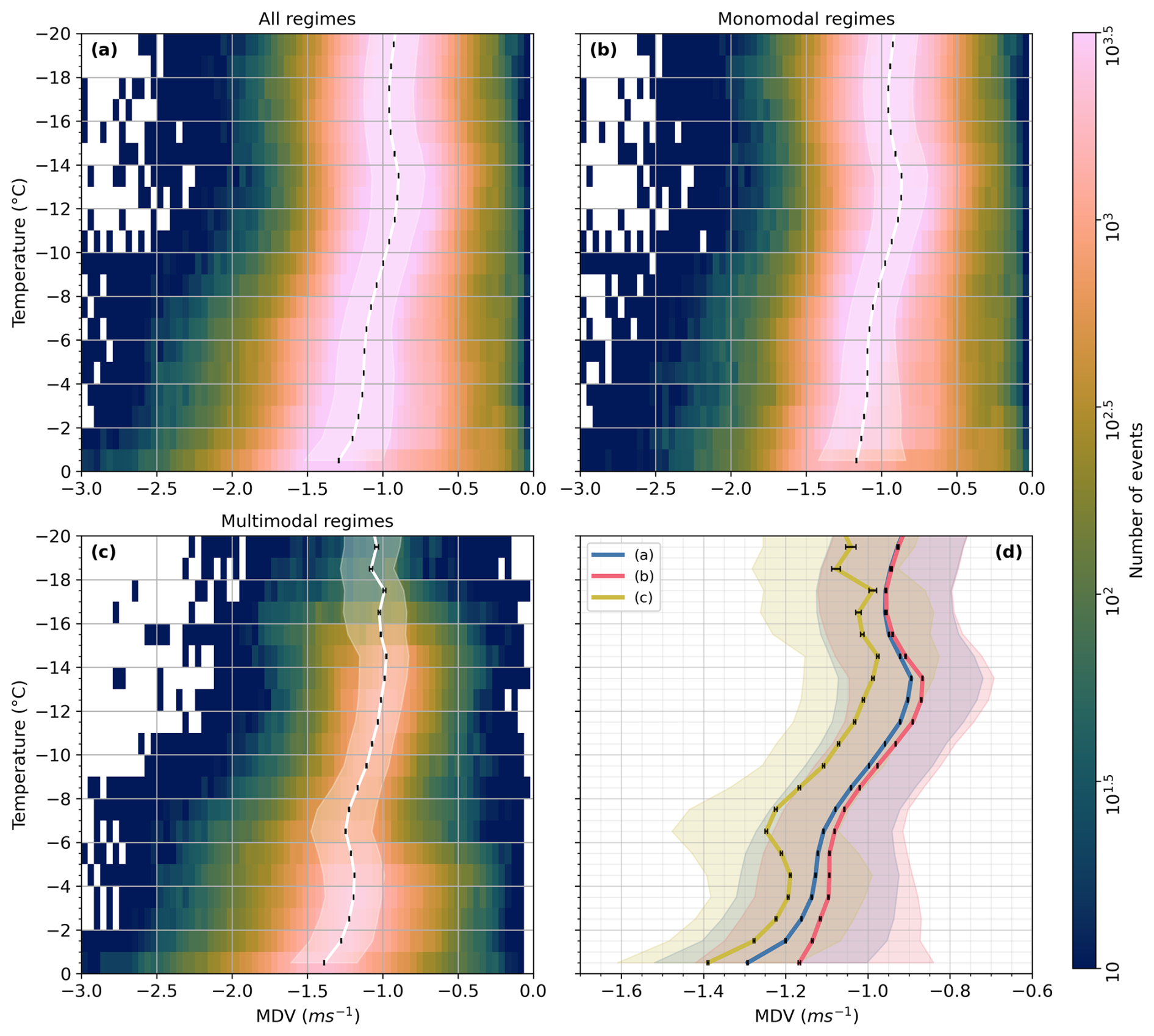
Figure 19 Vertical profiles of MDV as 2D histograms from all spectra (a), monomodal spectra (b) and multimodal spectra (c). The medians of each distribution are shown by the white line and interquartile ranges in panels (a)–(c). The medians and interquartile ranges of all distributions are shown in panel (d). The standard mean error, calculated as the width of the interquartile range divided by the square of the number of samples, is shown by the black bars. Note the logarithmic colour scale and change in x-axis limits in panel (d).

Previous remote sensing studies have aimed to characterise the vertical profile of MDV, and have suggested that on average it increases monotonically with increasing temperature. For example, Billault-Roux et al. (2023) calculate vertical profiles of MDV from Doppler radar for separate coexisting particle populations, and demonstrate that this variable generally follows a monotonically increasing profile for the primary particle mode, with small variations at temperatures close to 0 °C. The vertical MDV profile of the secondary modes show greater variation between cases, both in magnitude and profile shape. However, these results were shown for relatively short time periods (in the order of 20 to 30 min), where short lived but high-frequency random air motions such as turbulence or gravity waves may influence results (Protat and Williams, 2011). Another example is the statistics of MDV from Doppler radar data presented by Wiener et al. (2024). The data were collected over a 7-year period in Antarctica and the statistics show that the observed MDV in these cases follows a monotonically increasing profile. However, the profile of MDV is calculated against height, meaning smaller scale features in the this profile may be smoothed by varying vertical temperature profiles in different atmospheric conditions. Westbrook and Illingworth (2009) show findings from a continuous sample of stratiform ice clouds over 17 months that the vertical velocities of ice crystals relative to a 1.5 µm Doppler lidar have a strong temperature dependence; particles fall faster at higher temperatures which indicates the influence of particle growth and aggregation. However, close inspection of Fig. 3 in Westbrook and Illingworth (2009) shows that it is possible to see a fractional decrease (∼ 0.05 m s⁻¹) in the average lidar Doppler velocity at around −16 °C. Using the same dataset, Westbrook et al. (2010) investigate the fall speeds of specularly reflecting ice crystals in layer clouds; these are assumed to be planar crystal types, such as plate-like and dendritic crystals. The distribution of fall speeds of specularly reflecting particles demonstrates that instead of systematically increasing with temperature, there is a reduction in particle velocity at approximately −13 °C (see Fig. 13 in Westbrook et al., 2010). As these statistics are shown for specularly reflecting crystals, and this temperature is within the DGL, it is reasonable to suggest that the dominant crystal type at this temperature is dendritic. This feature is not discussed by Westbrook et al. (2010), but rather is treated as evidence of the velocity distribution of specularly reflecting crystals being slower and having a weaker variation with temperature compared to the statistics shown for “normal” (i.e. non-specularly reflecting) ice cloud in Westbrook and Illingworth (2009). However, comparisons with results shown in Figs. 18 and 19 suggest that the results shown by Westbrook et al. (2010) are in fact in agreement with the idea that dendritic crystals, whether pristine dendrites or precipitating particles with dendritic growth, consistently fall more slowly than different crystal types in other temperature regimes.

There have been different explanations in literature for observations of decreased MDV in the DGL. One suggestion is that the presence of a slow-falling secondary ice mode acts to decrease the observed MDV (Schrom and Kumjian, 2016). An alternative interpretation (Zawadzki, 2013) suggests that these changes at −15 °C are driven by ascending air motion at that level. However, our observation of multimodal spectra at this temperature over many events seems inconsistent with this idea as it is not obvious why ascent would be concentrated at that particular temperature. Our data is dominated by frontal clouds formed by large-scale ascent, which occurs over a wide range of temperatures. Another explanation suggests that enhanced depositional growth in the DGL causes latent heat release that is sufficient to increase buoyancy and consequently cause upward air motion (Zawadzki, 2013; Schrom and Kumjian, 2016). von Terzi et al. (2022) test these interpretations by analysing spectral edge velocities and conclude that the reduction in MDV is the result of new particle formation with low vertical velocities combined with the presence of a weak updraft likely caused by latent heat release from enhanced depositional growth. Our results instead demonstrate that changes in the primary population typically govern this decrease in MDV.

4.5 Discussion of mechanisms for multimodality

In Fig. 17, we show that there are two temperature regimes in which multimodal spectra are frequently detected. These temperature regimes are located between approximately −8 and −3 °C, where up to 40 % of spectra are multimodal, and between approximately −18 and −10 °C, where up to 20 % of spectra are multimodal. Whilst relatively little research into ice multiplication has focussed on frontal clouds, Mammatt et al. (2026) show findings from aircraft observations of a frontal case study that multimodal particle size distributions (PSDs) at −5 °C were likely to be caused by rime splintering in the case analysed. Two flight segments were analysed at −5 °C, one with significant liquid water content (LWC) but infrequent observations of drizzle-sized drops, and one without significant LWC. Analysis of particle shape in the segment with liquid water showed results consistent with the presence of two distinct particle populations coexisting in the same cloud volume, along with observations of needle crystals which were significantly higher in concentration than the expected ice nuclei concentration (DeMott et al., 2010). Ice particle concentrations in the segment where liquid water was absent were consistent with primary nucleation. Based on these observations, it is reasonable to suggest that neither ice-ice collisional fragmentation nor droplet fragmentation was the dominant source of small particles in this case. Given that the case studies described in Table 2 were selected to represent similar cloud types (i.e. stratiform frontal clouds), it may be reasonable to suggest that rime splintering is also active at similar temperatures in many or all of the cases analysed here. However, some care is needed in this interpretation as small particles produced by any mechanism, whether primary or secondary ice production, within this temperature range of around −8 to −3 °C would be likely to grow rapidly by vapour diffusion into a distinct population of needle-like and columnar crystals; it is therefore nearly impossible to definitively state which ice production mechanism is dominant based on observations alone.

The frequent detection of multimodal spectra between −18 and −10 °C is more puzzling. In Figs. 18 and 19, we show that there is a local minimum in the velocity of the primary population in the DGL; we suggest is caused by growth of dendritic branches on particles falling from higher altitudes, which acts to increase their drag and reduce the fall speeds of those particles. One possible explanation for the formation of the secondary mode in this temperature regime is that secondary particles are created by collisions between ice particles. Dendritic branches are thin and one could imagine that they could therefore break away from the rest of the ice particle or shatter into smaller fragments on impact (Grzegorczyk et al., 2023, and references therein). Once detached, these fragments will grow from vapour into new ice particles, producing a new population of slow-falling secondary particles which grow and sediment faster as they evolve and settle through the DGL. These will appear as a slow mode in the Doppler spectra with the velocity of this secondary peak increasing in magnitude as they fall to lower altitudes, consistent with our observations. The breaking off of these dendritic branches would reduce the surface area of the particle, and collisions between particles could lead to aggregation; both of these processes may cause an increase in the vertical velocity of the primary population as a result.

Weighing against this interpretation is the observation that the local minimum in Doppler velocity in the DGL is observed systematically in monomodal spectra as well as multimodal spectra. In fact, Fig. 19 shows that this minimum is more pronounced in monomodal cases than in multimodal ones. If dendritic arms are growing on particles precipitating from above in these monomodal cases, why do collisions between them not form secondary particles?

One possible explanation could be that particle concentrations are systematically lower in monomodal spectra compared to multimodal spectra. This would mean that the number of collisions between particles is also lower, preventing sufficient break off of dendritic branches to form a clear secondary mode. Particles then slow down more in monomodal spectra compared to in multimodal spectra because the dendritic branches causing greater air resistance are less likely to break off.

An alternative hypothesis is that the secondary production process involves riming, and our data provides some evidence to suggest this is the case. When we examine the velocity of the primary population in multimodal spectra, it is systematically higher than the primary velocity in monomodal spectra, which suggests that the processes involved in the formation of the multimodal population are also conducive to increasing the vertical velocity of the primary population. Riming is an effective mechanism to increase the fall speed of snowflakes (Garrett and Yuter, 2014; Moisseev et al., 2017). The existing literature on rime splintering is focussed on the temperature window near −5 °C, where Hallett and Mossop (1974) report hundreds of secondary ice particles produced per milligram of rime. However, close examination of their Fig. 2 reveals a slower (but non-zero) production rate of a few tens of splinters per milligram of rime at −13.5 and −15.5 °C. If those findings are accurate, then our measurements could potentially be explained by a (relatively slow) rime splintering process in the DGL.

The uncertainty surrounding both the mechanism producing multimodal spectra and mechanism causing the observed decrease in primary population velocity in the DGL demonstrates the importance of further research into the microphysical processes active at these temperatures. In particular, ice multiplication and aggregation processes involving dendritic particles remain poorly understood. For example, if increased drag force against pristine dendritic crystals causes a decrease in velocity, what happens when dendritic crystals aggregate – does the velocity increase due to the increased mass, or does the velocity remain similar or continue to decrease due to increased air resistance? Despite recent efforts to improve parameterisation of the terminal velocities of aggregated snowflakes, including aggregates comprised of dendrites (e.g. Dunnavan, 2021; Vázquez-Martín et al., 2021; Donovan et al., 2025; Seifert et al., 2026), the answer to this question remains unclear. Are the rime splintering or ice-ice fragmentation mechanisms efficient enough at low temperatures in non-turbulent clouds to cause one fifth of all spectra at these temperatures to be multimodal? One way to approach this further research is to use detailed super-particle models such as that developed by Brdar and Seifert (2018), combined with extensive scattering databases and radar forward operators such as that detailed by von Terzi et al. (2026), which link microphysics with radar observables.

If the analysis presented here were to be repeated on a different dataset, it could be developed further by utilising polarimetric radar data; polarimetric data were not available for the cases analysed here. Polarimetric data can provide insights into the properties of the particles in the observed cloud volume. For example, the linear depolarisation ratio (LDR) can be used to infer the shape of particles; high values of LDR imply the presence of needle or column crystals, whereas planar crystals correspond to low values of LDR (e.g. Oue et al., 2018; Billault-Roux et al., 2023). Likewise, values of differential reflectivity (ZDR) and specific differential phase (KDP) close to zero can be used to infer an active riming process (Oue et al., 2018). Another avenues of future work which arise from this work may include using lidar based techniques or machine learning based methods (Schimmel et al., 2022) to identify liquid water. It would also be interesting to investigate whether cloud top height or temperature has an impact on the number of modes identified or location of multimodality, or whether multimodal signatures are different between clouds associated with cold and warm fronts.

The implications of the findings presented in this study are apparent for NWP, where ice microphysical processes are crudely represented. For example, some models have no parameterisation in place to represent SIP (Wilson and Ballard, 1999; ECMWF, 2024), and those that do are usually focussed on rime splintering (Korolev and Leisner, 2020). Ice microphysical processes such as SIP have significant influences on cloud development and inaccurate representation can cause large errors in forecast process rates (Mammatt et al., 2026), thus demonstrating the importance of continued efforts to better understand these fundamental processes.

5 Conclusions

We have used radar Doppler spectra from 23 case studies to analyse the distribution of multimodal spectra in midlatitude frontal clouds. We have presented a method for detecting multimodal spectra using a peak finding algorithm, which is applied to the case studies. Results from two cases are shown to demonstrate the variability in the selected cases, and to show qualitatively how the spatial distribution of multimodal spectra changes between cases. The results from the peak finding algorithm enable us to quantitatively estimate the distribution of multimodal spectra with temperature; whilst there is no clear method to quantify the errors caused by inaccurate peak detection due to the unique nature of each Doppler spectrum (Shupe et al., 2004), we believe this to be a conservative estimate based on relatively strict turbulence and peak finding thresholds. We find there are two distinct temperature regimes where multimodal spectra are frequently detected. The first of these is between −3 and −8 °C where up to 40 % of spectra are multimodal, which is consistent with the temperatures at which rime splintering occurs. Indeed, Mammatt et al. (2026) investigate the final case study used in this work (Table 2) in greater detail, and show aircraft observations which support the idea that coexisting populations of dendritic crystals and needle crystals are responsible for producing multimodal PSDs, which are likely to produce the multimodal spectra observed. It is reasonable to assume that the same microphysical processes may be active in the majority of cases studies selected for the analysis presented in this paper, as they were chosen to represent clouds similar to the one analysed in Mammatt et al. (2026). The other temperature regime where multimodal spectra are frequently observed is between temperatures of −18 and -10 °C, where up to 20 % of spectra are multimodal. The mechanism responsible for the multimodal spectra detected at this temperature is unclear, but we suggest is likely to be caused by SIP.

The peak finding algorithm also returns the velocity corresponding to the peak spectral reflectivity for each Doppler spectrum, from which we produce the vertical profile of peak particle population velocities. These results can be separated into profiles for monomodal spectra and multimodal spectra, and suggest that there is a consistent decrease in particle velocity at temperatures around −13 °C in monomodal spectra; we hypothesise that this is caused by increased drag against particles with open geometry such as those with dendritic growth. The velocity of the primary population in multimodal spectra is higher than that in monomodal spectra, and the decrease in particle velocities at −13 °C is less apparent. Similar analysis can be performed for MDV, which can be separated for monomodal and multimodal spectra. Similarly to the particle velocity, a minimum in MDV is observed at −13 °C in monomodal spectra, and MDV from multimodal spectra is consistently higher than from monomodal spectra. This suggests that the conditions conducive to forming multimodal spectra are also conducive to growing the primary population. The mechanism behind this is unclear, but may be a result of riming or collisions between ice particles. As it is not possible to prove the occurrence of microphysical processes such as SIP and riming solely from radar observations, (Lauber et al., 2021; Luke et al., 2021; Li et al., 2021), the continued uncertainties surrounding the mechanisms active in frontal stratiform clouds demonstrates the importance of continued research into secondary ice production, especially at temperatures outside of the rime splintering regime, and processes active in the DGL.