Plume emission rate estimation using Gaussian plumes in remote imaging spectroscopy with SPIIRE

The detection and quantification of methane and other trace gas emissions using remote sensing with imaging spectroscopy is an increasingly important tool for understanding local, regional, and global emissions. Traditional algorithms for quantifying the emission rate often rely on user-determined, instrument-dependent parameters and arbitrary plume boundaries. In this paper we present a new algorithm to estimate the emission rate based on a statistical inversion of a physical, Gaussian plume model that does not depend on such parameter choices or plume boundaries, termed SPIIRE. The method fully exploits instrument noise models, incorporates surface-albedo and atmospheric effects present in gas enhancement imagery, and is well suited for operational use. We present simulation results showing improved noise resilience, demonstrate performance against controlled-release experimental data using AVIRIS-3 and EMIT, and provide multiple examples using EMIT. The controlled-release results show improved performance of SPIIRE relative to an IME-based method. We then show how the model can be extended to complex scenes having overlapping plumes and to spatially-distributed sources like landfills.

1 Introduction

In recent years, there has been tremendous progress in the detection and quantification of methane and other trace gas emissions through airborne and spaceborne imaging spectroscopy. This evolution has transitioned from initial demonstrations (Thorpe et al., 2013; Thompson et al., 2016) to robust monitoring capabilities (Cusworth et al., 2024; Zhang et al., 2025) within just a decade. These advancements have spurred the development of capabilities for existing missions, exemplified by NASA's Earth Surface Mineral Dust Source Investigation (EMIT) (Thorpe et al., 2025), and have led to the creation of innovative orbital instruments such as the Carbon Mapper Coalition Tanager-1 (Duren et al., 2025). Additionally, ongoing and completed controlled gas release experiments (Thorpe et al., 2021; Ayasse et al., 2023; Reuland et al., 2026) have demonstrated the ability of these technologies for quantifying emissions.

A variety of emission rate quantification methods exist, as described in (Jacob et al., 2022), for example, ranging from workhorse Integrated Mass Enhancement (IME) methods, described below in more detail, to more recent machine-learning based methods (Jongaramrungruang et al., 2022; Roberts et al., 2026). Many such methods are applied to overhead imagery of trace-gas concentration and assume constant emission rates and constant, spatially uniform wind. These assumptions imply that the total mass flux of gas remains constant across any cross-wind slice of the atmosphere downwind of the emission source. IME-based methods rely on these assumptions to infer an emission rate by converting the estimated concentration length of the gas plume relative to the background atmospheric concentration, or the “gas enhancement,” into the mass enhancement for each pixel. The mass enhancement is then summed over all pixels within the plume to create the IME which is then multiplied by the wind speed divided by the plume length. This results in the estimated emission rate in mass emitted per unit time (Frankenberg et al., 2016; Thorpe et al., 2023; Varon et al., 2018; Duren et al., 2019; Brodrick et al., 2026; Varon et al., 2020; Irakulis-Loitxate et al., 2021; Guanter et al., 2021; Sánchez-García et al., 2022; Roger et al., 2024; Kim et al., 2025; Li et al., 2026). For simplicity, in the remainder of this paper we define the IME method to follow Brodrick et al. (2026), although we note that the specific implementation and choice of parameters used in IME methods can generate significant variability in the estimates.

However, significant challenges persist in determining which pixels should contribute to the IME and how to accurately measure plume length. Plume boundaries are often defined through a combination of human input and basic image processing techniques, leading to variability in emission estimates based on subjective decisions. For example, Brodrick et al. (2026) uses the predetermined plume origin to seed a threshold-and-refine algorithm to identify a plume mask for the IME. Plume length can be calculated in a variety of ways, ranging from the longest dimension of the plume mask (Brodrick et al., 2026) to the square root of the mask area (Varon et al., 2018). Some authors choose to compensate for potential errors in the plume length measurement using an “effective” wind speed in which the wind speed is modeled as a parameterized function that is fit to either simulation results or experimental data. The effective wind speed is also used to compensate for turbulence, angular acquisition configuration (Gorroño et al., 2026), plume mask criteria and other similar effects. Consequently, IME-based methods frequently depend on tuned parameters that can significantly influence emission estimates and may require adjustments for different instruments, platforms (such as airborne versus spaceborne), collection geometries (Gorroño et al., 2026) or environmental conditions. Although these parameters can be and have been tuned using experimental data, the challenge of acquiring such data for orbital systems, along with the calibration process itself, remains a fundamental issue for IME-based approaches.

Gaussian plumes have been extensively utilized in the literature for both plume modeling and emission rate estimation. The derivation typically assumes a point source emitting into a constant wind with turbulent diffusion effects incorporated by treating the downwind Gaussian width as a parameterized function of distance. Historically, the determination of these width parameters has relied on estimates of the atmospheric state, as detailed by Seinfeld and Pandis (2016), who derive Gaussian plumes and present various turbulent spreading models. Notable examples of emission rate estimation using Gaussian plumes include Krings et al. (2011), who analyzed overhead airborne data with multiple narrow passes through individual plumes, Fioletov et al. (2015), who applied Gaussian plumes to estimate SO₂, and Shah et al. (2019), who employed multiple vertical and horizontal samples at a single downwind location. Three recent studies – Nassar et al. (2021), Kuhlmann et al. (2024), and Pang et al. (2025) – adapt Gaussian plumes to gas enhancement imagery, each differing in their methodologies. While none of these studies employ a probabilistic framework, Kuhlmann adapts the spreading parameters to the data and utilizes a flexible plume. In contrast, both Nassar and Pang use straight plumes with fixed spreading parameters, with Nassar's based on wind speed (see Sect. 2.2 of Nassar et al., 2021).

In this paper, we present a Maximum Likelihood Estimation (MLE) method for emission rate estimation utilizing Gaussian plume models (Seinfeld and Pandis, 2016; Varon et al., 2018) called Statistical Plume Imaging Inversion for Rate Estimation, SPIIRE. Our approach estimates parameters directly from the data, comparing the plume model to the observed gas enhancement imagery to assess the likelihood that the measured data represents a noisy realization of a Gaussian plume. A numerical optimizer is used to determine the parameters that maximize this likelihood, or equivalently, minimize the weighted model-data error. This method adapts a physical plume model to observational data, demonstrating robustness against instrument noise and surface albedo effects, while minimizing reliance on user-specific or instrument-specific parameters.

SPIIRE incorporates three key features that collectively ensure accurate model fits. First, it estimates all parameters within a turbulent Gaussian plume model directly from the data, including those related to downwind spreading. Second, the Gaussian plume is designed to be flexible in the cross-wind direction, allowing it to adapt to the observed plume as it aligns with local topography and variations in wind direction. Lastly, the probabilistic MLE framework takes into account variable detection sensitivity caused by local atmospheric and surface albedo effects, downweighting noisy, low-signal pixels during optimization based on their known uncertainties (Fahlen et al., 2024). Together, these enhancements yield quantitative models of observed plumes while minimizing the subjectivity associated with manual plume delineation.

More complex scenarios that challenge IME-based approaches include plume complexes (Duren et al., 2019; Sánchez-García et al., 2022; Thorpe et al., 2023) and area sources (Cusworth et al., 2024; Maasakkers et al., 2022; Zhang et al., 2025; Marjani et al., 2024). Plume complexes consist of multiple apparent sources whose plumes merge or overlap, complicating the ability of IME-based methods to discern which gas enhancements should be attributed to each source. This overlap can also obscure the identification of plume length, potentially introducing significant errors. Pang et al. (2025) propose a novel approach for estimating emissions from plume complexes by employing a Gaussian plume inversion to “separate” overlapping plumes, allowing an IME-based strategy to be applied to each plume individually. Area sources, such as landfills, emit gas over a relatively large and contiguous area, often lacking a distinct downwind tail. These sources frequently do not meet the assumptions inherent in IME-based methods, resulting in diminished accuracy.

The Gaussian plume model can effectively address these challenges by simultaneously modeling multiple plumes. Overlapping plumes can be easily accommodated by summing the concentrations of multiple Gaussian plumes and optimizing each plume's parameters concurrently. Area sources can similarly be represented by clustering several Gaussian plumes within a small region surrounding the source and optimizing their parameters to ensure that the combined forward model accurately reflects the observed enhancement. Initial examples of these generalizations are shown Sect. 4.2 and 4.3 but more work is needed to demonstrate the accuracy of the emission rates in these cases.

The paper is organized as follows: Sect. 2 details the 2D Gaussian plume inversion method, Sect. 3 describes results, including simulated plumes and controlled release results, and Sect. 4 extends the method to overlapping plume complexes and distributed sources. Section 5 provides discussion, including consideration of wind speed estimation, and is followed by conclusions in Sect. 6.

2 Plume Model Inversion

2.1 Gaussian Plume Models

A simple model for the concentration C of a gas emitted from a point source and carried in the wind is the Gaussian plume model, defined by

$$\begin{array}{}\text{(1)}& C(x,y,z)={\displaystyle \frac{Q}{u}}{\displaystyle \frac{\mathrm{1}}{\sqrt{\mathrm{2}\mathit{\pi }}{\mathit{\sigma }}_y}}{e}^{-\frac{y^{\mathrm{2}}}{\mathrm{2}{\mathit{\sigma }}_y^{\mathrm{2}}}}{\displaystyle \frac{\mathrm{1}}{\sqrt{\mathrm{2}\mathit{\pi }}{\mathit{\sigma }}_z}}{e}^{-\frac{(z-z_{\mathrm{0}}{)}^{\mathrm{2}}}{\mathrm{2}{\mathit{\sigma }}_z^{\mathrm{2}}}},\end{array}$$

where ($x,y,z$) is a right-handed coordinate system with positive z normal to the Earth's surface and x increasing in the direction of the wind speed vector which was assumed constant in space and time in Eq. (1)'s derivation (Seinfeld and Pandis, 2016). The plume origin is assumed to be at $(x,y)=(\mathrm{0},\mathrm{0})$. Because we will simply integrate over z in the following section, we use an overly-simplistic vertical distribution that assumes that all the gas is above the surface, or z₀≫σ_z, for convenience. The quantity Q is the gas emission rate, typically in units of kg h⁻¹, and u is the wind speed.

The plume spreading parameters are denoted by σ_y and σ_z and are generally functions of the downwind position x. A variety of spreading models and parameterizations exist for Gaussian plume models (Carrascal et al., 1993). A particularly common model is to assume that

$$\begin{array}{}\text{(2)}& {\mathit{\sigma }}_y\left(x\right)=a{\left({\displaystyle \frac{x}{d}}\right)}^b.\end{array}$$

Different authors find different values for parameters a, b, and d and often recommend that they change with wind speed or atmospheric state (like those of the Pasquill-Gifford atmospheric state models in, for example, Seinfeld and Pandis, 2016). In this work, we take d = 1000 m and allow the fitting procedure described below to find the values of a and b that best match the data. The choice of 1000 m follows Varon et al. (2018) but, based on the parameterization in Eq. (2), this choice is arbitrary and only for convenience in comparing the retrieved parameters a and b to previous work (Carrascal et al., 1993). Importantly, the spreading model we propose does not include an explicit dependence on the wind speed. This means that the wind speed only appears in the ratio $Q/u$. As a result we cannot estimate Q separately from u, but only their ratio, which we call C_Q below. For convenience, we use units of kg h⁻¹ per m s⁻¹ for C_Q as Q is typically kg h⁻¹ while u is m s⁻¹. Again, we ignore σ_z as will become clear shortly.

Standard Gaussian plumes assume constant wind, but we can accommodate some wind direction variation by allowing the cross wind mean to vary as a function of the downwind position, as in $C_{\text{2D}}(x,y)\to C_{\text{2D}}(x,y-m(x\left)\right)$. Since many plumes appear to bend in the wind, this addition provides the model with the flexibility needed to obtain good fits, as will be seen below, and reduces the potential error associated with model-data mismatch. We leave the problem of relieving the inconsistency of allowing directional variation without a magnitude change to future work (but see Sect. 5 for a discussion regarding simultaneously estimating the wind magnitude). We parameterize this variation with a piecewise linear function defined by parameters m_x spaced at 3 times the Ground Sampling Distance (GSD) in the along wind x-direction. Previous work with Gaussian plumes has allowed wind variation using Bezier curves (Kuhlmann et al., 2024), but we have found that the piecewise linear function works well for the relatively high-spatial-resolution data used below. We have also found that the emission estimate is not very sensitive to this choice. The number of m_x parameters is the number that fit from the plume origin to the far end of the retrieval region.

2.2 Maximum Likelihood Estimation of Emission Rate

We seek to estimate C_Q by comparing the Gaussian plume model with the remote measurements. In the remainder of the paper, we assume that prior processing of the observations has estimated the concentration length ${\widehat{l}}_{i,j}$ in ppm m, where i,j are spatial pixel indices, and that potential plumes have been detected and queued for emission rate estimation. Since this data is a 2D overhead map of the gas concentration, the comparison requires adapting the 3D model to the 2D remote measurement by integrating over the z direction, giving the 2D Gaussian model

$$\begin{array}{}\text{(3)}& C_{\text{2D}}(x,y)={\displaystyle \frac{Q}{u}}{\displaystyle \frac{\mathrm{1}}{\sqrt{\mathrm{2}\mathit{\pi }}{\mathit{\sigma }}_y}}{e}^{-\frac{y^{\mathrm{2}}}{\mathrm{2}{\mathit{\sigma }}_y^{\mathrm{2}}}}.\end{array}$$

In performing the integration, we assume that all the gas is above the surface (z₀≫σ_z).

To facilitate the comparison of the model to the data, we seek a probabilistic treatment for the measurement following Fahlen et al. (2024). In that work, it is shown that the concentration length in each pixel can be treated as a Gaussian random variable (not to be confused with the Gaussian plume model). It is also shown that the estimated concentration length is biased from the true concentration length by local albedo and atmospheric variation, an effect quantified by the “sensitivity”. Both the sensitivity and the pixel's concentration length uncertainty can be calculated from the observation. We adapt this model to create a maximum likelihood estimator for the parameters of the Gaussian plume model of Eq. (3). To do so, we model the concentration length in each pixel as a Gaussian random variable and define its mean to be the Gaussian plume model in Eq. (3) scaled by the sensitivity. In this formulation, the concentration length measurement in each pixel is considered to be a realization of the corresponding random variable, with the measurement in highly uncertain pixels being more likely to deviate from the plume model than those in less uncertain pixels. We therefore obtain the probability distribution function in each pixel

$$\begin{array}{}\text{(4)}& p_{C_{\text{2D}}}\left({\widehat{l}}_{i,j}\right)={\displaystyle \frac{\mathrm{1}}{\sqrt{\mathrm{2}\mathit{\pi }{S}_{i,j}^{\mathrm{2}}{U}_{i,j}^{\mathrm{2}}}}}{e}^{-\frac{({\widehat{l}}_{i,j}-\mathrm{2}k{S}_{i,j}{C}_{\text{2D}}(x_i,y_j){)}^{\mathrm{2}}}{\mathrm{2}{S}_{i,j}^{\mathrm{2}}{U}_{i,j}^{\mathrm{2}}}},\end{array}$$

where S_i,j and U_i,j are the sensitivity and uncertainty, at pixel (i,j). The factor k, which converts the model from area concentration [kg m⁻²] to concentration length [ppm m], is 10⁶ (m³ mol⁻¹) (mol kg⁻¹). In the rest of this paper, we consider methane plumes near the surface at standard temperature and pressure (STP), yielding k≈ 1.4 × 10⁶ ppm m³ kg⁻¹. The factor of 2 in the exponent's numerator is to account for the light's path through the plume. Although this factor in principle depends on the look and solar angles along with the plume's cross-sectional shape and height above the ground, even including double plumes (Gorroño et al., 2026; Sánchez-García et al., 2022), we assume that the concentration length measurement in each pixel represents a double path through the plume: down from the sun then back up from the ground.

To estimate C_Q, we form the likelihood of the plume model parameters θ∈Θ given the data, given by

$$\begin{array}{}\text{(5)}& \mathrm{\Lambda }\left(\mathit{\theta }\right)=\prod _{i,j\in P}{p}_{C_{\text{2D}}}\left({\widehat{l}}_{i,j};\mathit{\theta }\right),\end{array}$$

and then seek the values of those parameters that maximize the likelihood, as in

$$\begin{array}{}\text{(6)}& \widehat{\mathit{\theta }}={\text{arg\hspace{0.17em}\hspace{0.17em}max}}_{\mathit{\theta }\in \mathrm{\Theta }}\mathrm{\Lambda }\left(\mathit{\theta }\right).\end{array}$$

The product in Eq. (5) is taken over all pixels inside the plume and surrounding area. In the results below, we define P to be all the pixels within the rectangular window that bounds the manually-delineated plume plus a 10 pixel buffer on all four sides. For the EMIT data used here, we rely on the plume boundaries that are part of the standard EMIT products (Brodrick et al., 2026). The AVIRIS data has no publicly available plume boundaries as of this writing, so we created them following the EMIT procedure. All the plume images below show the entire retrieval region P (except the right side of Fig. 8, which is zoomed for visual clarity). The advantage of including pixels beyond the manual delineation is twofold. First, we eliminate the subjectivity necessarily associated with drawing a boundary around the apparent plume by allowing the optimization to determine the plume shape without arbitrary restrictions. Second, we allow the method to take advantage of the region of gas enhancement beyond the apparent end of the plume. Although not visibly associated with the plume and therefore not included in the manual delineation, the model may predict gas enhancement here and its presence can be exploited by the likelihood formulation. We limit the buffer to 10 pixels both to limit computational time but also to reduce the likelihood that the plume model be degraded by inadvertently including scene artifacts that may be mistaken as true gas enhancements. The presence of the uncertainty in the denominator of the exponent in Eq. (4), when combined over P in Eq. (5), effectively downweights uncertain pixels. As the downweighting is relative to the neighboring pixels, this feature of SPIIRE is most helpful for plumes that span high and low-albedo regions (see Fig. 7 for example) rather than weak plumes that are only barely detectable. The parameter space Θ includes the wind-normalized emission rate C_Q and the spreading parameters a and b, a rotation α about the plume origin to allow for arbitrary wind directions, and the m_x plume bending parameters. Because the Gaussian plume model is derived for point sources, the concentration becomes infinite at the origin as the spreading model shrinks. In the implementation here, we work around this problem by forcing the origin to always lie on a pixel boundary that is excluded from P. However, a different spreading model σ_y or, ideally, a more physical plume model based on a finite-sized gas vent, could achieve a similar effect.

We use the SciPyBoundedMinimize optimizer provided in the jaxopt python library (Blondel et al., 2021). The initial value for the wind direction is computed as the line from the manually-determined plume origin to the centroid of the plume boundary. In practice, we optimize the log likelihood to simplify the cost function and we estimate ln C_Q and ln a to keep the numerical range of those parameters similar to that of the others.

The uncertainty in the emission rate Q depends on many factors, including instrument noise and wind speed. These two can be combined using standard error propagation methods based on the expression Q=uC_Q, yielding

$$\begin{array}{}\text{(7)}& {\mathit{\sigma }}_Q^{\mathrm{2}}={\left({\mathit{\sigma }}_{C_Q}{\displaystyle \frac{\partial Q}{\partial C_Q}}\right)}^{\mathrm{2}}+{\left({\mathit{\sigma }}_{\mathrm{u}}{\displaystyle \frac{\partial Q}{\partial u}}\right)}^{\mathrm{2}}.\end{array}$$

We calculate ${\mathit{\sigma }}_{C_Q}$ using the Cramer-Rao bound (Van Trees, 2004) and σ_u as the standard deviation of the surrounding wind samples following Brodrick et al. (2026). Another source of error is due to the mismatch between the true plume and the Gaussian model, but this is difficult to quantify. The use of the sensitivity and the m_x help to reduce this error, but the uncertainty persists, meaning that the above expression for uncertainty likely underestimates the true uncertainty. For further discussion, see Sect. 3 for empirical evidence regarding the uncertainty.

The principal limitations of SPIIRE are the challenge of estimating wind speed and the difficulty in fully quantifying the detrimental effects of applying SPIIRE to non-Gaussian plumes. The former is discussed below in Sect. 5.1. Regarding the latter, we suggest a path forward in Sect. 4.3 in which we generalize the model to adapt to apparently non-Gaussian plumes. Other limitations include the requirement for a parameterized downwind spreading model σ_y, the unknown 3D shape of the plume and the light's path through it (the 2 in Eq. 4) (Gorroño et al., 2026), and numerical difficulties associated with the optimization.

3 Results

We demonstrate SPIIRE using both airborne AVIRIS-3 (Coleman et al., 2026) and space-borne EMIT (Green et al., 2023) methane enhancement data (Brodrick et al., 2026). Although we use methane emissions throughout as a test case, we note that the method could apply equally well to other atmospherically stable gases or even to aerosol plumes. Both instruments are pushbroom imaging spectrometers with a spectral range of approximately 380–2500 nm and 7 nm spectral resolution. EMIT's swath width is approximately 80 km with 60 m spatial resolution. AVIRIS-3's equivalent, being an airborne sensor, is variable depending on the flight altitude but its spatial resolution ranges from approximately 0.5 to 6 m for the data used here. For both instruments, a column-by-column spectral matched filter is used on the calibrated radiance data to estimate the methane concentration length in each spatial pixel (Thorpe et al., 2017; Thompson et al., 2015) along with its sensitivity (bias) and uncertainty (Fahlen et al., 2024). The EMIT data can be found following Thorpe et al. (2025) and the AVIRIS-3 data following Chlus et al. (2024).

3.1 Simulated Data

A main advantage of SPIIRE is that the optimization region P is large and extends beyond the visible plume enhancement, allowing the model to smoothly respond to local variation and reducing the estimator's susceptibility to measurement noise. To demonstrate SPIIRE's resilience to measurement noise, we simulated 600 plumes using the 2D Gaussian plume model with random C_Q and spreading parameters but with no bends (the simulated m_x are all 0). We choose to simulate Gaussian plumes because they satisfy the assumptions of both IME methods and SPIIRE and therefore provide a test of the enhanced noise performance. The simulated C_Q are uniformly distributed between 200 and 3000 kg h⁻¹ per m s⁻¹ to span a typical range of emission rates and wind speeds observed with EMIT. The plumes are injected (added) into random locations in 263 randomly chosen EMIT methane enhancement scenes that have previously been determined to have no clouds or true emissions (see Figure 8 of Fahlen et al. (2024) for injection details). We include the local sensitivity when injecting the simulated plume into the noisy data. Figure 1 shows the simulation results by comparing the IME method on the left with SPIIRE on the right. As expected, SPIIRE has superior noise performance (reduced uncertainty) as demonstrated by its narrower vertical spread and is unbiased over the full range. We note that it may be difficult in practice to realize the full noise improvement as data-model mismatch will inevitably occur due to unmodeled effects like changing winds, local topography variation, intermittent sources, and so on. However, these effects often plague IME-based methods too, making SPIIRE's noise resilience an important contribution.

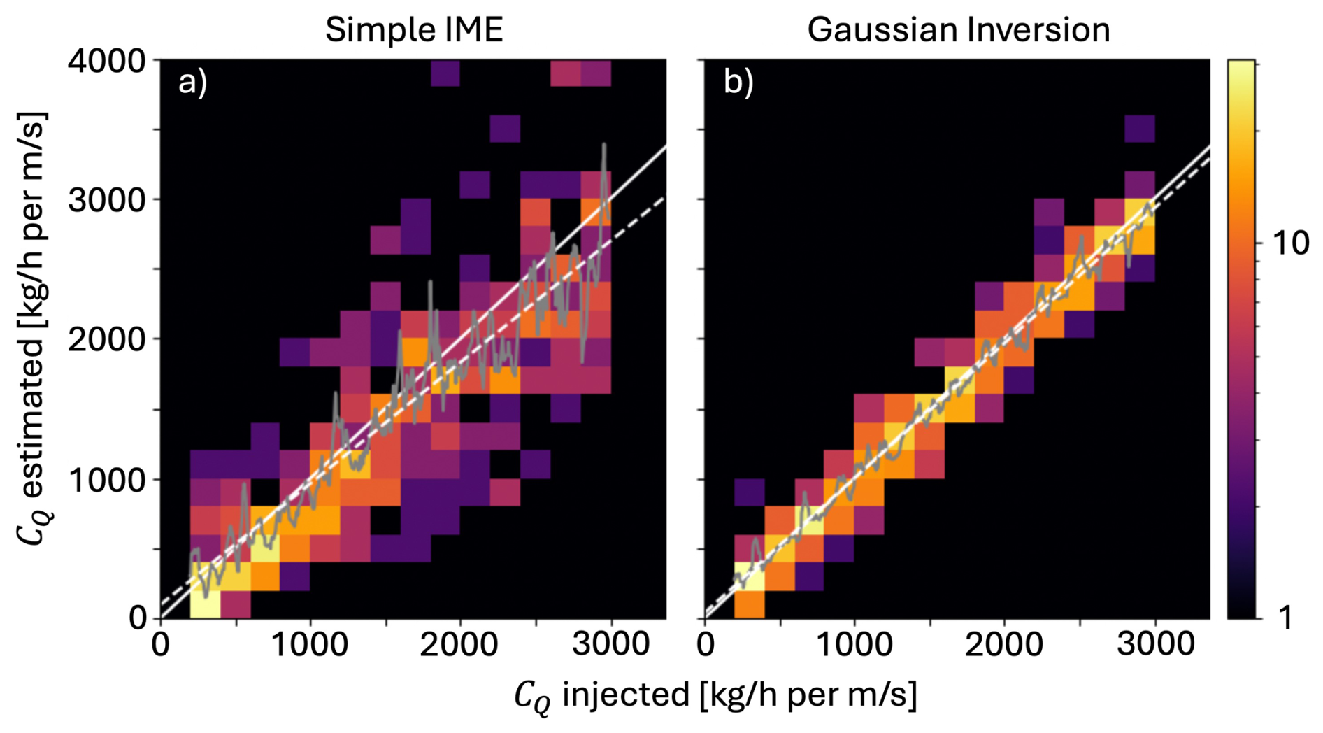
Figure 1 Histograms showing the estimated C_Q along the vertical axis and the injected C_Q along the horizontal for (a) the IME method and (b) SPIIRE. The solid white line is the one-to-one line, the dashed white line is the linear regression, and the gray line is the moving average.

3.2 Controlled Release Results

We demonstrate the accuracy of SPIIRE using controlled-release experimental data (Duren et al., 2025). Following the approach in El Abbadi et al. (2024), methane is released and accurately measured from a point 7.3 m above ground at two different sites: Casa Grande, AZ at (32.822° N, 111.785° W) and Evanston, WY at (41.275° N, 110.930° W). AVIRIS-3 performed 110 passes at Evanston on 11–14 September 2024 and 34 passes at Casa Grande on 4–5 November 2024. EMIT observed the site during 7 overpasses. Wind speeds and directions are measured at 2 and 10 m above ground using a sonic anemometer.

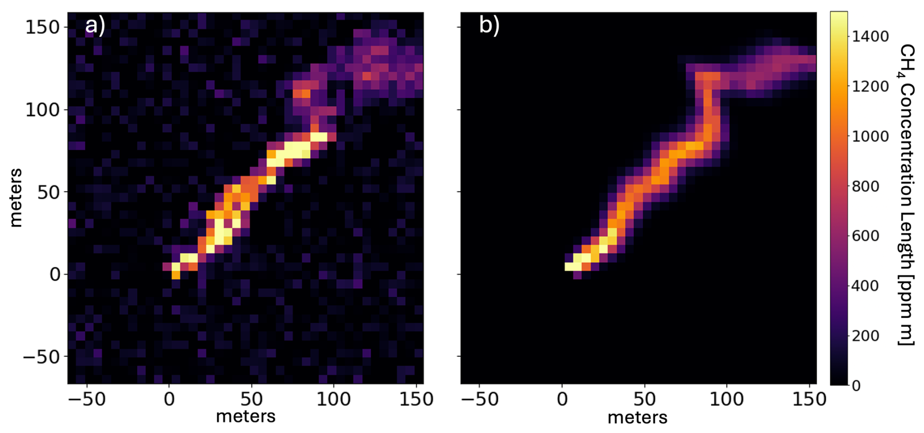
Figure 2 AVIRIS-3 SPIIRE example from the 4 November 2024 controlled release experiment. Figure (a) shows an image of estimated concentration length, and (b) shows the fit 2D Gaussian model plume with sensitivity correction. The metered emission rate is 155 kg h⁻¹ and the estimated rate is 165 ± 27 kg h⁻¹ with an approximately 4 m s⁻¹ wind speed. AV3 flightline AV320241104t183250. The figure, and all subsequent plume images, depicts the entire retrieval region P.

An example plume is shown in Fig. 2 using AVIRIS-3 data from 4 November 2024 at Casa Grande, Arizona (AV320241104t183250). As mentioned previously, the retrieval region P includes all pixels in the rectangular region within 10 pixels of the widest part of the plume in all directions (all pixels shown in Fig. 3a). The adapted Gaussian plume model is shown in Fig. 3b with the sensitivity correction applied. The bending of the plume model to accommodate apparent wind direction changes in the plume is achieved through the m_x. A key feature of the method is the modification of the model by the sensitivity to account for surface- and atmospheric-related biases, although this effect is modest at the mostly-uniform experimental site.

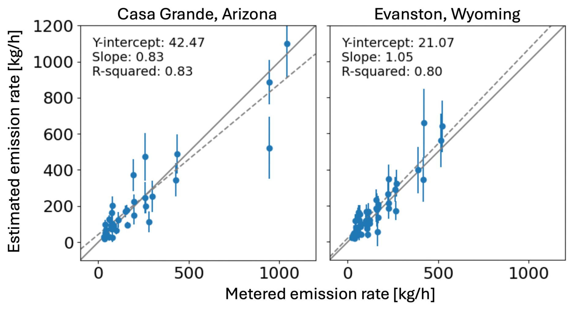
Figure 3 Emission rate estimates using SPIIRE on the AVIRIS-3 Arizona (left) and Wyoming (right) controlled release experiment data collections. The one-to-one line is solid gray while dashed gray indicates the linear regression through all points. In calculating the emission rate, the wind speed from the 2 m tower was used after averaging over the preceding 30 s. We note that results vary depending on the choice of tower and smoothing period. The percentage of emission estimates that are within the uncertainty is 50 % and 62 % for the Arizona and Wyoming locations, respectively.

The emission rates from SPIIRE are plotted against the metered emission rate for the two AVIRIS-3 controlled release experiments (Duren et al., 2025) in Fig. 3. We have removed several overpasses where the plumes are too weak to be credibly detected. The linear fit is shown in dashed gray with the fit statistics inset. The wind speeds used are from the 2 m sonic anemometer. Both the wind speeds and the metered emission rates are the mean over the preceding 30 s relative to the overpass time. We chose 30 s because it represents a reasonable propagation time for the range of plumes included in the experiment while providing sufficient smoothing. For both experimental locations, the estimated emission rates are accurate in the aggregate with a reasonable spread about the true emission rate. The IME method, shown in Fig. 4, yields similar but slightly worse performance, driven in part by outliers whose estimates are sensitive to the particular choices of implementation and parameter. We note that uncertainty in the wind speed and decisions about how it is processed affect the comparisons too.

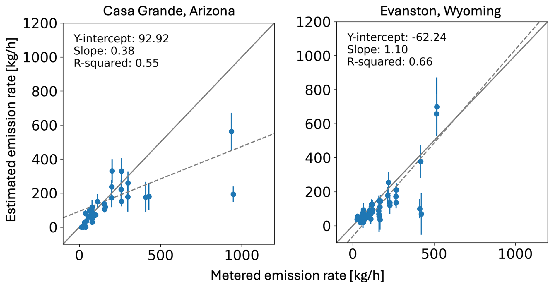
Figure 4 Emission rate estimates using IME on the AVIRIS-3 Arizona (left) and Wyoming (right) controlled release experiment data collections. The one-to-one line is solid gray while dashed gray indicates the linear regression through all points. In calculating the emission rate, the wind speed from the 2 m tower was used after averaging over the preceding 30 s. We note that results vary depending on the choice of tower and smoothing period. The percentage of emission estimates that are within the uncertainty is 44 % and 40 % for the Arizona and Wyoming locations, respectively.

The estimated emission rates for the EMIT controlled release experiment overpasses are shown in Fig. 5 for SPIIRE and Fig. 6 for IME. EMIT did not detect the first two despite relatively large metered emission rates, likely due to high winds during those collections (5.1 and 5.2 m s⁻¹, respectively). Because the releases only started a few minutes before the overpass, they are short compared to typical plumes, all between 8 to 16 EMIT pixels (< 1 km). This means that the assumptions guiding the decision to use a buffer region surrounding the visible plume do not hold here and we assume instead that the end of the apparent plume actually represents the end of the true gas enhancement. Accordingly, we modified the cost function for the five examples shown in Fig. 5 to include only the pixels within a circular region surrounding the emission source and whose radius matches the last visible portion of the plume. This choice reduces the number of pixels used in the retrieval and likely degrades the performance relative to that observed in the AVIRIS-3 data in Fig. 3. Nevertheless, the estimator's performance is good, with four of the five points within their uncertainty of the metered emission rate.

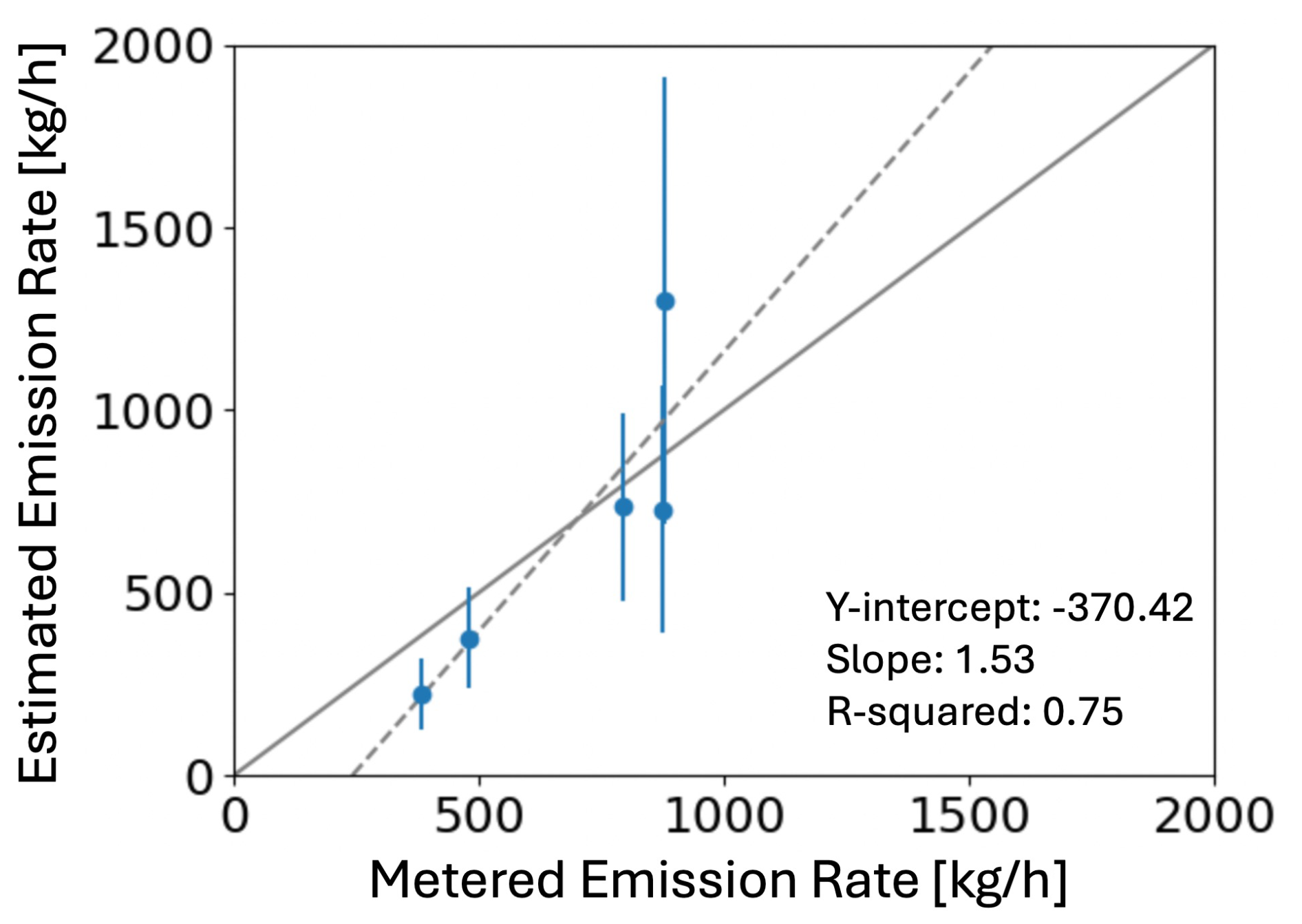
Figure 5 Emission rate estimates using SPIIRE on the EMIT Arizona controlled release experiment data collections. The one-to-one line is solid gray while dashed gray indicates the linear regression through all points. In calculating the emission rate, the wind speed from the 2 m tower was used after averaging over the preceding 30 s. We note that results vary depending on the choice of tower and smoothing period. The emission estimate for four of the five overpasses are within the uncertainty.

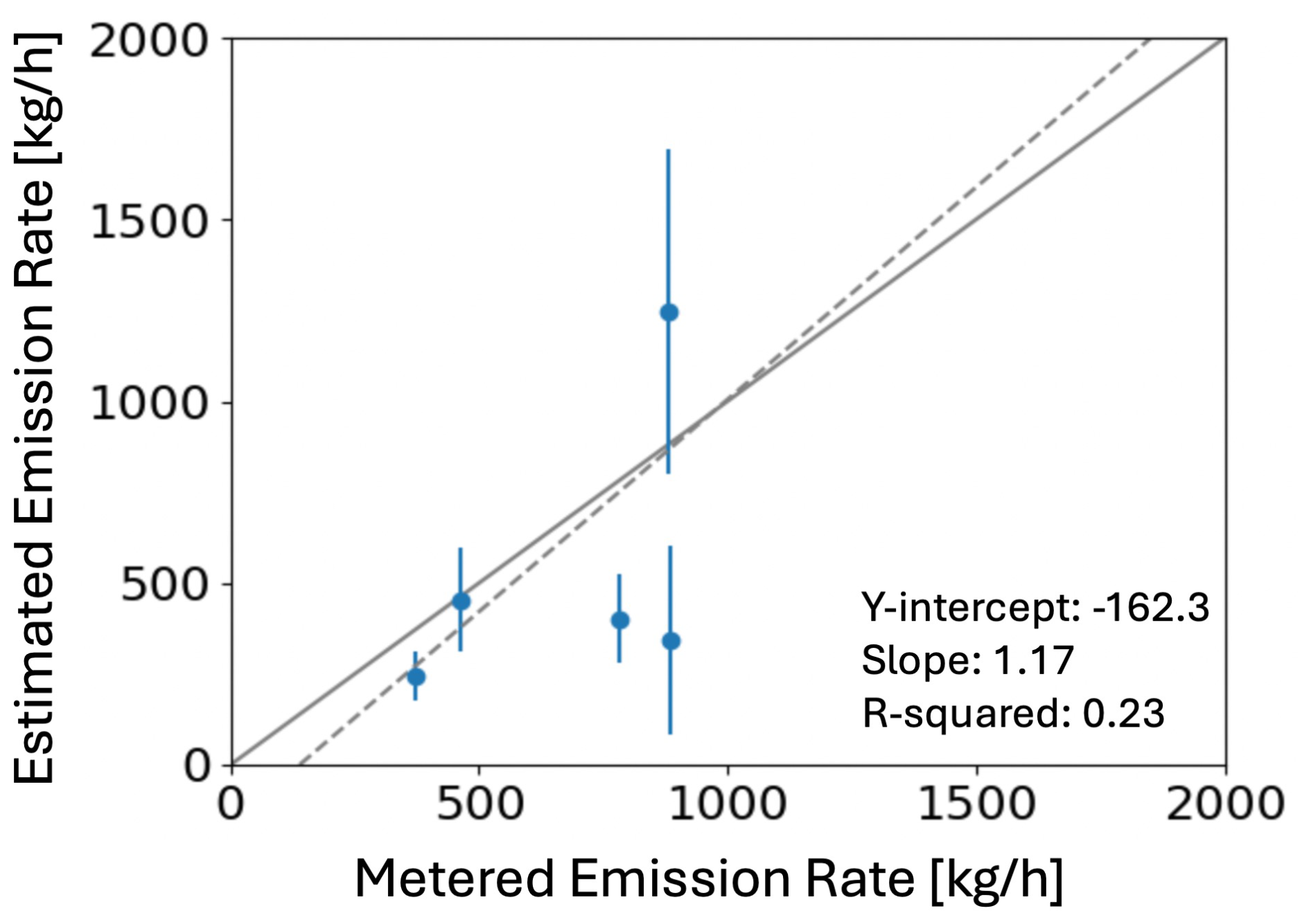
Figure 6 Emission rate estimates using IME on the EMIT Arizona controlled release experiment data collections. The one-to-one line is solid gray while dashed gray indicates the linear regression through all points. In calculating the emission rate, the wind speed from the 2 m tower was used after averaging over the preceding 30 s. We note that results vary depending on the choice of tower and smoothing period. The emission estimate for two of the five overpasses are within the uncertainty.

Section 2.2 noted that the uncertainty calculation in Eq. (7) and used in Figs. 3 and 5 neglects the uncertainty due to model-data mismatch because it is difficult to quantify. However, the experimental results provide a means to empirically assess the degree to which Eq. (7) underestimates the true uncertainty, at least for the point-source plumes provided by the experiment. We find that the emission rates fall within their uncertainty range of the true value in 50 %, 62 %, and 80 % of the overpasses at the AVIRIS Arizona, AVIRIS Wyoming, and EMIT Arizona sites, respectively. Since Eq. (7) represents a 1σ uncertainty, we would expect approximately 68 % of the overpasses to be within their uncertainty of the true emission rate if the uncertainty were not biased. The results indicate that neglecting model-data mismatch in the uncertainty calculation does not significantly bias the resulting uncertainty estimate.

We note that the IME method used to produce the estimates quoted throughout this paper requires a different set of user-defined parameters for the AVIRIS-3 results versus the EMIT results. This is to address the differences in spatial resolution and noise performance between the two instruments. It is possible to tune these parameters for AVIRIS-3 using the controlled release data, but the limited availability of such data for EMIT means that it is difficult to project the IME performance quoted above to EMIT observations. In contrast, the SPIIRE results throughout this work use the same set of parameters for both instruments, meaning that the validation shown here using AVIRIS-3 and EMIT controlled release data is more likely to apply to the full EMIT database, especially for point-source plumes like those in the experiment.

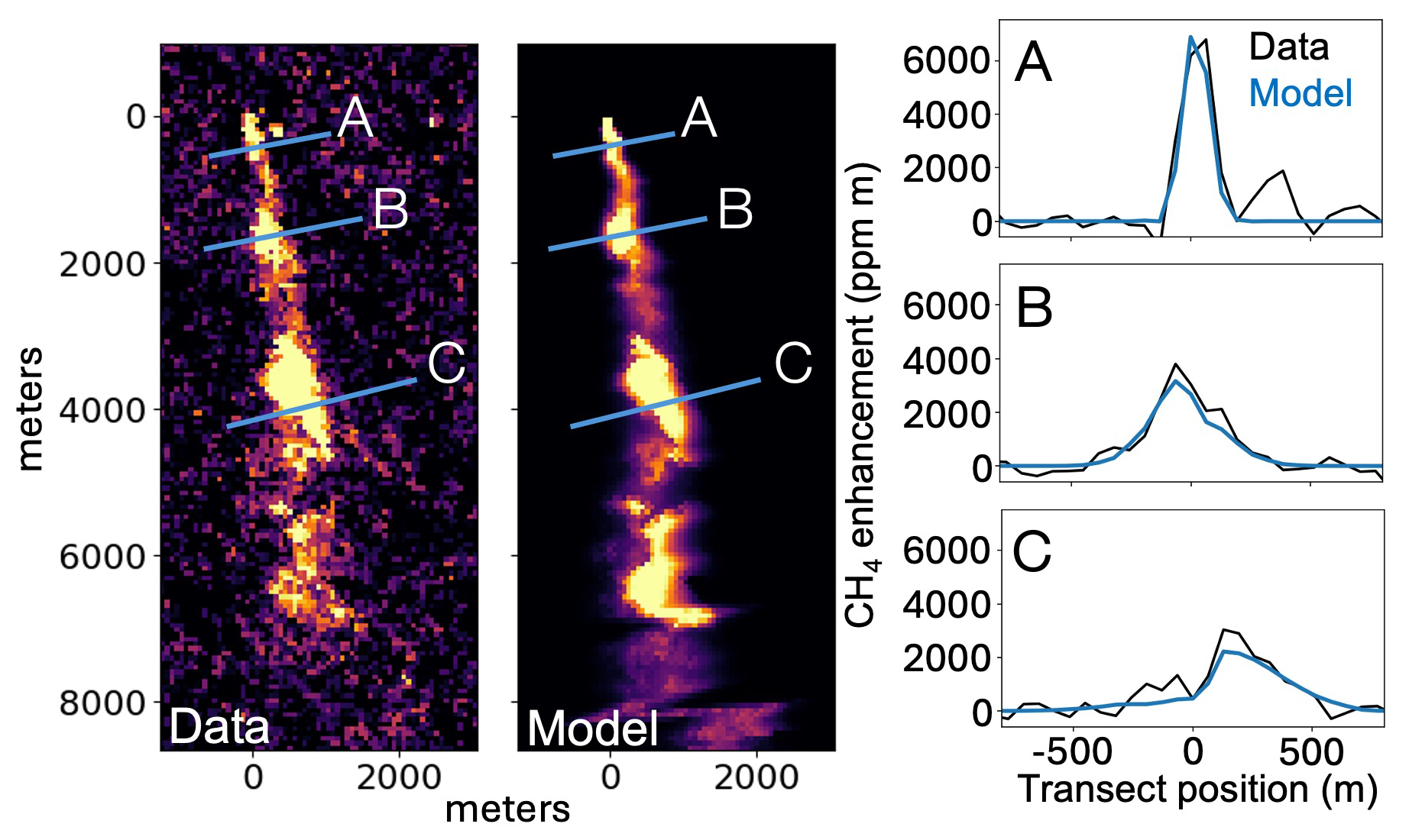
Figure 7 SPIIRE example from EMIT CH4_PlumeComplex-2794 from 28 February 2024 at 27.9686° N latitude and 69.8097° E longitude in Pakistan. From left to right: data image of estimated concentration length, fit 2D Gaussian model plume with sensitivity correction (color), and plots of three transects showing the data and the sensitivity-corrected model. The color scale is the same as that in Fig. 2. The IME emission rate estimate is 6997 ± 784 and the SPIIRE estimate is 9295 ± 1000 kg h⁻¹.

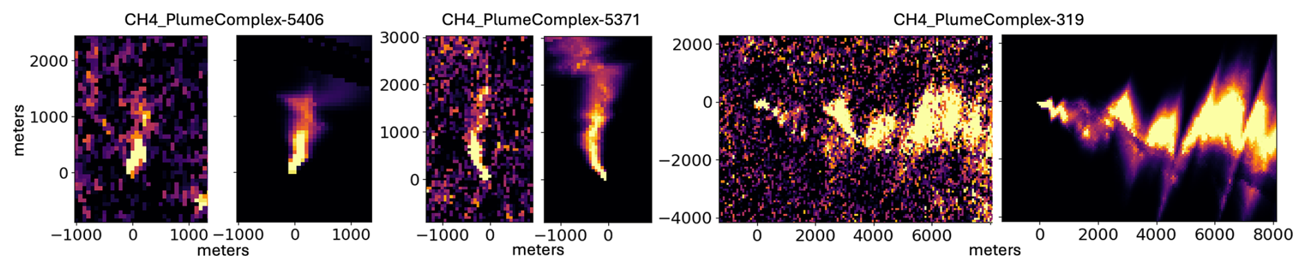
Figure 8 SPIIRE examples from EMIT plotted as in Fig. 2, left to right: CH4_PlumeComplex-5406 from 2 June 2025 at (49.490° N, 35.697° E), CH4_PlumeComplex-5371 from 17 July 2025 at (−21.968° N, 148.024° E), and a subregion of P for CH4_PlumeComplex-319 from 12 June 2023 at (41.437° N, −111.169° E). All three are likely oil and gas facilities. The IME estimates, left to right, are 1148 ± 65, 5619 ± 290, and 10 589 ± 874 kg h⁻¹, and the corresponding SPIIRE estimates are 1793 ± 101, 4596 ± 247, and 21 736 ± 1559 kg h⁻¹. The color scale is the same as that of Fig. 9.

3.3 Plume Modeling and Interpretation

A major benefit of SPIIRE is the improved understanding of visually-complex plumes. Figure 7 and the third example in Fig. 8 exhibit EMIT plumes whose initial appearance suggests an intermittent source or turbulent winds. We find instead that these plumes can be well modeled with a steady-state Gaussian plume that includes albedo effects through the sensitivity, suggesting that in some cases intermittency or turbulence need not be considered to understand complicated plume shapes. The cross-wind transects on the right side of the Fig. 7 demonstrate the quality of the plume modeling in this case. Although no ground truth emission rate is available for this plume, SPIIRE estimated Q at 3.4 times that of the IME method. This plume provides an example of the two methods diverging despite the plume appearing to be due to a point emission source. In this case the model-data agreement is good, suggesting SPIIRE's estimate is likely a more accurate representation of the true emission rate.

4 Applications

4.1 Isolated Plumes

IME-based methods are currently being used operationally and their emissions estimates are publicly available, including for example Duren et al. (2025); Thorpe et al. (2025), subject to quality control thresholds (Brodrick et al., 2026; Cusworth et al., 2024). SPIIRE could be readily incorporated into such workflows to augment the estimates and to provide the additional benefits of plume interpretation using the adapted 2D Gaussian model. As described in the following subsections, SPIIRE may also help to relieve the quality control thresholds by providing a new method to quantify otherwise challenging plumes in difficult environments. Three more SPIIRE examples from the EMIT database are shown in Fig. 8.

4.2 Overlapping Plume Complexes

IME-based approaches to plume emission rate estimation do not perform well in plume complexes having multiple apparent sources whose plumes merge downwind. In such cases it is impossible to know how to allocate CH₄ enhancement pixels to any particular source. However, it is straightforward to adapt SPIIRE to plume complexes by simultaneously inverting multiple plumes, with the model to be optimized simply the sum of each plume. Figure 9 shows an example EMIT scene having multiple apparent sources. Originally labeled CH4_PlumeComplex_4191, it is clear from a close examination of the data image at left along with high resolution base-layer imagery from Google Maps that there are in fact several point sources. The wind direction in this case appears to be coincidentally aligned so that the plumes overlap. We identify five independent point sources and simultaneously invert five corresponding Gaussian plumes. It is not necessary to assign the CH₄ enhancement in a particular pixel to any particular plume as the simultaneous inversion automatically adapts each plume to the data to provide a combined CH₄ model over the entire set of pixels in the figure.

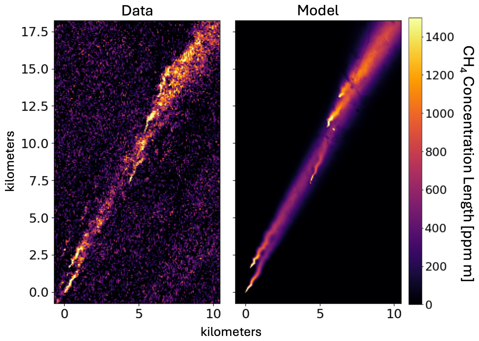
Figure 9 SPIIRE example from EMIT CH4_PlumeComplex-4191 from 1 February 2025 at 35.3551° N latitude and 40.3505° E longitude, likely an oil and gas site. The left plot shows the measured CH₄ enhancement and the right the fit 2D Gaussian model.

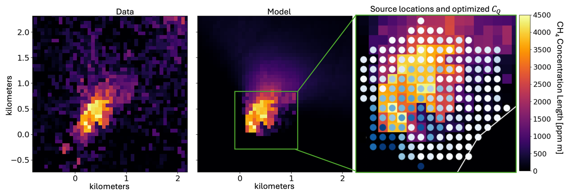
Figure 10 SPIIRE example from EMIT CH4_PlumeComplex-508 from 18 August 2022 at a landfill at 44.0395° N latitude and 87.8681° E longitude. The left plot shows the measured CH₄ enhancement and the middle the fit 2D Gaussian model with sensitivity correction. This plume is due to a landfill whose emissions are spread over several EMIT pixels. The right image shows the location of each point source in the model, with color indicating relative source strength: white represents no emission while dark blue is the maximum. The optimizer found that most sources have little or no emission. The combined emission rate is estimated to be approximately 11 000 kg h⁻¹ with a wind speed of 3.3 m s⁻¹.

4.3 Distributed Sources

Distributed, or area, sources are also challenging for IME-based quantification methods as they often do not appear to satisfy the assumptions needed to calculate the emission rate based on their IME. In particular, these sources often appear as amorphous enhancement regions spanning many pixels but without any apparent point source or long downwind tail. The plume in Fig. 10, showing a landfill in northwest China, is a good example. Using the Gaussian plume, we can model distributed sources as a collection of point sources spread over a predefined area and then allow the optimizer to individually determine each plume's C_Q. We assume that the wind speed is the same over the entire region, so we force each point plume to share the same spreading parameters. In the example shown in Fig. 10, we selected a polygon that covers the landfill and surrounding area using high-resolution Google Maps imagery. This region is approximately 800 m wide. The point sources within the polygon, one per pixel, are shown in the green inset on the right side of the figure with color indicating relative intensity. Specifically, white represents no emission and dark blue relatively high emission. The resulting optimized model is shown in the middle panel of Fig. 10. Intriguingly, the optimizer found that the data is best represented by a relatively few sources concentrated near the bottom left and middle of the enhancement region. The lack of downwind tail, a common feature of distributed sources, is also modeled well using the collection of point sources. The IME method yields an estimated emission rate of approximately 6200 kg h⁻¹ with a wind speed of 3.3 m s⁻¹ while the distributed point source model yields approximately 11 000 kg h⁻¹. Although it is possible that this method is susceptible to artifacts not compensated for with the sensitivity, we hope that future work can expand on this idea and demonstrate good performance over a large class of amorphous plumes commonly observed in plume databases.

5 Discussion

SPIIRE's accuracy on the experimental data shown in Figs. 3 and 5 suggests that the method could be operationalized to other gases and even aerosol plumes. We have performed the inversion using a single point source plume on the majority of the EMIT methane plume database with generally robust results provided the plumes satisfy the point source assumption. Following the quality control methods already in use (Cusworth et al., 2024; Brodrick et al., 2026), SPIIRE could directly augment IME estimates and be readily adapted to any type of emission, ranging from other gases (CO, NH₃, etc.) to aerosol plumes due to, for example, wildfires. The Gaussian model could also be generalized to model gases with short atmospheric lifetimes. For the many plumes that do not meet the point source assumption, the overlapping and area source models demonstrated in Sect. 4 present a path forward. More work is needed to use these operationally, however, especially in determining how many sources to use and where to put them. The example shown in Fig. 9 was relatively easy to manually identify the various sources, but this is often not the case, nor is manual identification a viable long-term solution. One potential path is suggested by the observation that the optimizer successfully avoided adding extraneous plumes in Fig. 10, suggesting that plumes could be seeded automatically at local maxima in the enhancement with the optimizer free to allocate source strengths. Alternatively, the distributed source model could be used for all plumes, although care must be taken to avoid increasing the dimensionality of the optimizer beyond what can be reasonably solved.

Apart from improvements in measurement precision, a major advantage of SPIIRE is that it alleviates the need for subjective plume boundaries. Even where workflows use automated ML-based plume segmentation to speed labeling, these systems are generally trained on human-labeled data and thus subject to the same human biases in the plume definition. In contrast, the 2D model is defined over an infinite geographic area, removing the boundary as a source of error. Only the plume origin need be identified. Thus, it would only require an automated system capable of finding plume origins to enable a fully automatic, end-to-end plume quantification capable of handling the enormous data volumes of next generation imaging spectrometers.

The advantages of the adapted plume model also include better knowledge of and resilience to turbulent wind effects that can distort the observed plume shapes and degrade the accuracy of IME-based approaches (Gałkowski et al., 2025). Although there is no doubt that turbulent winds can cause plumes to appear bunched up, Fig. 7 shows that in many cases what appear to be turbulent wind effects are in fact measurement artifacts that can be corrected in the retrieval. Additionally, SPIIRE is likely less sensitive to turbulent wind effects when they do occur for two reasons. To understand why, imagine a constantly-emitting source with small gas clouds that exceed the concentration predicted by a Gaussian plume model in some parts of the plume. Conservation of mass through the plume means that the excesses must also be accompanied by “holes” elsewhere. The algorithms that detect pixels to include in the IME calculation may fail to incorporate these holes, leading to a mismatch in the IME and fetch length and thus to errors in the emission rate estimate. SPIIRE, in contrast, fits the model through the gas clouds and holes, an averaging effect that smooths over the turbulence.

5.1 Wind Speed Estimation

A major challenge with emission rate quantification is in the estimation of the wind speed. Historically the wind speed has been derived from weather reanalysis data, like HRRR (Dowell et al., 2022) and ERA5 (Hersbach et al., 2020), but recent work using multiple observations separated by a few seconds provides an alternative based on the observation itself (Eastwood et al., 2025). A seemingly straightforward improvement to the method described above would be to simply simultaneously estimate the wind speed along with the other parameters, but, as mentioned in Sect. 2, the functional form of the standard plume model in Eq. (3) is degenerate in Q and u. Pang et al. (2025) attempt this, which may partially explain the poor performance that they obtained in their Gaussian plume inversions. Alternative models with more explicit dependence on wind speed exist, as in Eq. (4) of Kuhlmann et al. (2024), but these either have other degeneracies or are apparently nonphysical. We have not been able to generate meaningful results with them. We have also considered establishing a correlation between the retrieved spreading parameters a and b with the various studies that predict them using atmospheric stability classes (Pasquill-Gifford, for example, as in Seinfeld and Pandis, 2016; Carrascal et al., 1993). Unfortunately, the retrieved values for these parameters often exceed their published ranges making the correlation difficult to establish. We therefore leave simultaneous wind speed estimation for future work, especially the development of a physical plume model with explicit wind speed dependence that cannot be compensated by a nuisance parameter.

6 Conclusions

SPIIRE addresses key challenges in the field, including the subjective delineation of plume boundaries and the reliance on hard-to-determine parameters. By integrating a probabilistic framework, we enhance the reliability of emission rate estimations, allowing for better adaptation to real-world conditions. Moreover, the model's flexibility enables it to accommodate complex scenes with overlapping plumes and spatially distributed sources, providing a more comprehensive understanding of emission dynamics.

In summary, this paper aims to bridge the gap between methodologies and modern requirements for emission quantification, offering a robust, flexible, and user-independent approach. We demonstrate the effectiveness of our method through simulation results, controlled-release experimental data, and practical applications using different imaging spectrometers, highlighting its potential for widespread operational use in environmental monitoring. Additionally, the algorithm can be extended to estimate emission rates in complex scenarios involving multiple overlapping plumes and distributed sources, such as landfills.