Simultaneous temperature and wind profiling in the troposphere and lower stratosphere using a Rayleigh Doppler lidar with a Fizeau-interferometer-based high-spectral-resolution receiver

Simultaneous profiling of atmospheric wind and temperature is essential for investigating atmospheric dynamics and wave–mean flow interactions. However, conventional molecular Rayleigh lidar techniques generally retrieve temperature and wind using different measurement principles, such as hydrostatic integration for temperature retrieval and double-edge discrimination for wind measurement. Direct retrieval of both quantities from a single spectrally resolved molecular backscatter signal remains less commonly demonstrated, particularly in the troposphere and lower stratosphere. To explore this approach, we developed a high-spectral-resolution lidar (HSRL) receiver based on a Fizeau interferometer and a 32-channel linear photomultiplier-tube array. The receiver spatially resolves the Rayleigh–Brillouin (RB) spectrum across the detector array, enabling the Doppler shift and thermally induced spectral broadening to be determined from the same measured spectrum for joint wind and temperature retrieval without frequency scanning. Numerical simulations were first performed to optimize the spectral sampling characteristics of the receiver, identifying the 32-channel configuration as a favorable compromise between spectral resolution and signal-to-noise ratio (SNR) over the 2 to 20 km altitude range. Wind profiles were retrieved from 2 to 20 km with a temporal resolution of 10 min, while temperature profiles were retrieved from 5.3 to 20 km with a temporal resolution of 5 min. Temperature retrieval was performed where the Mie scattering signal fraction was below approximately 8 %, which corresponded to a lower retrieval altitude of about 5.3 km under the observed atmospheric conditions. The vertical resolutions were 60 m below 10 km and 300 m above 10 km. Compared with radiosonde measurements, the retrieved temperatures showed mean absolute temperature differences of 1.19 K at 5.3–10 km and 2.10 K above 10 km. Below 5.3 km, wind retrieval used model temperature as an auxiliary input, yielding mean absolute differences of 2.34 and 2.50 m s⁻¹ for the zonal and meridional wind components, respectively. In the fully lidar-based joint-retrieval region above 5.3 km, the corresponding wind differences were 1.84 and 2.97 m s⁻¹ at 5.3–10 km and 3.02 and 3.08 m s⁻¹ above 10 km. These results demonstrate that the proposed scan-free multichannel Fizeau-interferometer HSRL enables reliable temperature profiling from the middle troposphere to the lower stratosphere and extends wind measurements into the lower troposphere, while offering a compact spectral architecture with potential for future airborne and spaceborne Doppler lidar applications.

1 Introduction

Atmospheric temperature and wind are two fundamental state variables governing atmospheric dynamics and thermodynamics. Vertically resolved observations of these quantities are essential for studies of atmospheric waves and their interactions with the background circulation, for the evaluation and initialization of numerical weather prediction models, and for climate research. Radiosondes provide accurate in situ measurements of both temperature and wind but are generally limited in temporal resolution. Lidar, in contrast, offers continuous remote sensing with high temporal and vertical resolution and has therefore become an important tool for profiling atmospheric temperature and wind over extended altitude ranges.

A variety of lidar techniques have been developed for atmospheric temperature and wind measurements. Conventional Rayleigh temperature lidar retrieves temperature from molecular number-density profiles through hydrostatic integration and has been widely used for observations of the middle atmosphere (Hauchecorne and Chanin, 1980; Kaifler and Kaifler, 2021). Its application toward lower altitudes, however, becomes increasingly challenging because aerosol Mie scattering contaminates the molecular return and introduces biases into the retrieved density and temperature profiles. Rotational Raman lidar provides an alternative approach for tropospheric temperature profiling because the temperature dependence of the relative intensities of rotational Raman lines can be exploited without relying on hydrostatic integration (Behrendt and Reichardt, 2000; Behrendt et al., 2002; Radlach et al., 2008), although the relatively weak Raman scattering signal generally limits the achievable measurement range and temporal resolution. At higher altitudes, resonance lidar can extend temperature observations into the mesosphere and lower thermosphere (Alpers et al., 2004; Wang et al., 2026). Atmospheric wind, on the other hand, can be measured by Doppler wind lidar through the frequency shift of light backscattered from molecules or aerosols. Direct-detection Doppler wind lidar based on molecular scattering has been demonstrated from ground-based, airborne, and spaceborne platforms (Garnier and Chanin, 1992; Dou et al., 2014; Liu et al., 2026; Witschas et al., 2022a; Liu et al., 2002). Nevertheless, the RB spectrum contains information on both atmospheric motion and thermodynamic state: its spectral displacement is determined by the line-of-sight (LOS) Doppler velocity, whereas its spectral shape and width depend primarily on atmospheric temperature and pressure. Therefore, spectrally resolving the RB scattering signal provides the possibility of retrieving wind and temperature from the same measured spectrum.

High-spectral-resolution detection techniques have therefore been developed to resolve the spectral characteristics of molecular backscatter and extract the atmospheric information encoded in the RB spectrum. These techniques employ frequency-selective optical elements to convert the spectral characteristics of the molecular backscatter signal into measurable intensity or spatial distributions.

Considerable progress has been made in exploiting RB scattering for atmospheric temperature measurements. Early laboratory measurements of spontaneous Rayleigh–Brillouin scattering in nitrogen, dry air, and moist air were reported by Witschas et al. (2010), who compared the measured ultraviolet line shapes with the Tenti S6 model (Witschas et al., 2010). Accurate forward modeling of the RB spectrum is commonly based on the Tenti S6 model, which has been extensively investigated under atmospherically relevant temperature and pressure conditions (Hua and Kobayashi, 2005; Witschas et al., 2014a). Analytical approximations have also been developed to reduce the computational burden associated with repeated evaluation of the RB spectrum while maintaining sufficient spectral accuracy for atmospheric retrieval (Witschas, 2011a, b). Using a frequency-scanning Fabry–Perot interferometer, Witschas et al. (2021, 2016, 2014b) demonstrated daytime atmospheric temperature measurements from resolved RB spectra and subsequently extended the technique to airborne measurements (Witschas et al., 2021, 2016, 2014b). Hair et al. (2001) demonstrated the feasibility of iodine-vapor-filter HSRL for temperature retrieval using the Tenti S6 model while strongly suppressing aerosol scattering (Hair et al., 2001).

Although frequency scanning enables detailed reconstruction of the RB spectrum, sequential spectral sampling increases measurement time and system complexity and may be disadvantageous for rapidly varying atmospheric conditions or moving platforms (Liu et al., 2019). To overcome this limitation, Xu et al. (2020, 2021) developed an imaging high-spectral-resolution lidar receiver based on a Fizeau interferometer and a linear photomultiplier-tube (PMT) array. In this configuration, different spectral components are mapped onto different detector channels so that the complete RB spectrum can be recorded simultaneously without frequency scanning. Field measurements demonstrated tropospheric temperature profiling from 4.0 to 9.2 km with a temporal resolution of 5 min and a vertical resolution of 300 m, with systematic temperature errors below 3 K and random uncertainties of approximately 1.7–2.3 K (Xu et al., 2020; Xu et al., 2021). Such a multichannel imaging configuration is particularly attractive for atmospheric measurements because it converts the instantaneous optical spectrum directly into a spatially resolved intensity distribution.

Fizeau interferometers are also well suited to Doppler frequency measurements (McKay, 2002). They have been investigated in direct-detection atmospheric wind lidar systems (Bu et al., 2006) and were implemented as the Mie spectrometer of the Atmospheric Laser Doppler Instrument (ALADIN) aboard the Aeolus satellite, where Doppler frequency shifts of narrowband aerosol and cloud returns were converted into spatial displacements on the detector (Witschas et al., 2022b; Vaughan et al., 2025). These developments demonstrate the capability of Fizeau interferometers to encode spectral frequency information into spatial detector signals with high sensitivity and stability. When combined with a scanning lidar telescope, LOS Doppler measurements obtained at different viewing azimuths can further be combined to retrieve horizontal wind components. This capability is particularly important for atmospheric dynamics applications, for which zonal and meridional winds rather than a single LOS velocity are generally required.

Concepts for simultaneously retrieving atmospheric wind and temperature from high-spectral-resolution molecular scattering have been proposed and investigated previously. However, practical implementation remains challenging for several reasons. First, the receiver must resolve both the displacement and the shape of the RB spectrum with sufficient spectral sampling and SNR over a broad altitude range. Second, simultaneous wind and temperature retrieval constitutes a coupled inverse problem because spectral displacement and spectral broadening must be distinguished under measurement noise, aerosol contamination, and changing atmospheric conditions. Iterative spectral-fitting methods can therefore suffer from slow convergence, sensitivity to initial values, or unstable solutions at low SNR. Third, a single LOS measurement provides only the projected wind velocity, whereas retrieving physically useful horizontal wind vectors requires integration of the spectral receiver with a multi-directional scanning lidar system. A measurement architecture that combines scan-free full-spectrum acquisition, stable joint spectral inversion, and multi-azimuth wind measurements would therefore provide an important step toward operational simultaneous profiling of atmospheric temperature and vector wind.

In this study, we develop a multichannel Fizeau-interferometer HSRL receiver and integrate it into a scanning Doppler wind lidar previously developed at the University of Science and Technology of China (USTC). The receiver employs a 32-channel linear PMT array to spatially resolve the atmospheric RB spectrum in a single acquisition without frequency scanning. The Doppler displacement of the spectrum is used to determine LOS wind velocity, while its temperature-dependent spectral shape provides the information required for temperature retrieval. The scanning telescope directs the lidar beam toward different azimuthal directions, allowing multiple LOS measurements to be combined and thereby enabling retrieval of the zonal and meridional wind components.

In addition to the receiver development, a fast iterative retrieval algorithm is developed for the joint inversion of wind and temperature from the measured multichannel RB spectrum. The algorithm is designed to accelerate convergence while improving the robustness and stability of the coupled wind–temperature retrieval, particularly under varying SNR conditions. Numerical simulations are first used to optimize the receiver configuration, including the number of detector channels and the wedge angle of the Fizeau interferometer, and to characterize the retrieval performance. The complete system is subsequently evaluated through field measurements in Urumqi, China. Wind profiles are retrieved over an altitude range of 2–20 km, while fully lidar-based simultaneous wind and temperature retrieval is demonstrated from 5.3 to 20 km, with the lower altitude limit determined by a Mie scattering signal fraction below approximately 8 %. The retrieved zonal and meridional wind components and temperature profiles are evaluated against radiosonde measurements. The results demonstrate a measurement framework that combines scan-free multichannel RB spectroscopy, multi-directional Doppler wind sensing, and fast iterative joint retrieval, providing a compact and robust approach for simultaneous atmospheric wind and temperature profiling and a potential receiver architecture for future ground-based, airborne, and spaceborne Doppler lidar systems.

2 Measurement Principle

The measurement principle of the designed HSRL receiver is shown in Fig. 1. The atmospheric backscattering spectrum collected by the telescope, consisting of molecular RB scattering and aerosol Mie scattering, passes through the Fizeau interferometer and produces equal-thickness interference fringes. The spectral distribution is thereby converted into a spatial intensity distribution on the linear PMT, enabling multichannel photon collection without frequency scanning.

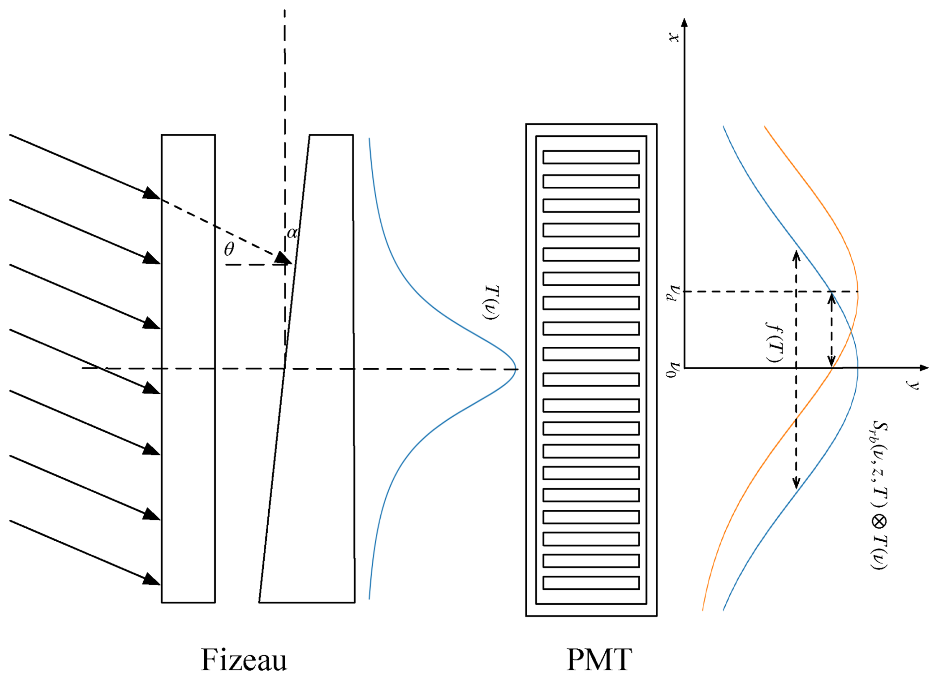
Figure 1 Schematic diagram of simultaneous wind and temperature measurement by Fizeau interferometer.

When temperature and wind information are extracted from the molecular RB spectrum, the two parameters are intrinsically coupled. The atmospheric temperature determines the width and detailed shape of the Rayleigh–Brillouin spectrum, whereas the line-of-sight wind velocity introduces a Doppler frequency shift of the spectrum. After spectral-to-spatial conversion by the Fizeau interferometer, both effects jointly modify the intensity distribution recorded by the linear PMT. Therefore, temperature and Doppler frequency shift must be retrieved simultaneously through spectral fitting rather than independently.

2.1 Wind measurement

Wind velocity is gained through fringe technique. A multibeam Fizeau wedge achieves static spectral scanning by means of varying distance between two plates of wedge. Following Mckay, the Fizeau fringe can be approximated by an Airy function given in Eq. (1) when the form factor S<0.6 (McKay, 2002), where S is calculated using Eq. (2).

$$\begin{array}{}\text{(1)}& {\displaystyle }A\left(\mathit{\varphi }\right)={\displaystyle \frac{{\left(\mathrm{1}-R\right)}^{\mathrm{2}}}{\mathrm{1}-\mathrm{2}R\cos \left(\mathit{\varphi }\right)+R^{\mathrm{2}}}},\text{(2)}& {\displaystyle }S=F_R{\left({\displaystyle \frac{\mathrm{2}{L}_{\mathrm{0}}{\mathit{\nu }}_{\mathrm{0}}{\mathit{\alpha }}^{\mathrm{2}}}{c}}\right)}^{\frac{\mathrm{1}}{\mathrm{3}}},\end{array}$$

In Eq. (1), R is the reflectance of the inner surface, ϕ is the phase factor, $\mathit{\varphi }=\mathrm{4}\mathit{\pi }L\mathit{\nu }/c$ which is related to the plate spacing L and the frequency of incident light. In Eq. (2), L₀ is the plate spacing at the center, ν₀ is the frequency of the laser, α is the wedge angle, F_R is the finesse of the Fizeau interferometer which can be calculated as: $F_R=\mathit{\pi }\sqrt{R}/(\mathrm{1}-R)$. Due to the wedge angle between the two optical plates, there are different spacings L at different positions of the Fizeau interferometer. Taking the center point of the Fizeau interferometer as the coordinate origin, where x=0 (according to Fig. 1), the expression for spacing L can be obtained as: $L=L_{\mathrm{0}}-\mathit{\alpha }x$. In summary, the relationship between the stripe position x and the frequency shift ν_d can be derived as follows:

$$\begin{array}{}\text{(3)}& x={\displaystyle \frac{{\mathit{\nu }}_{\mathrm{d}}{L}_{\mathrm{0}}}{\mathit{\alpha }\left({\mathit{\nu }}_{\mathrm{0}}+{\mathit{\nu }}_{\mathrm{d}}\right)}},\end{array}$$

According to the Doppler effect of light: ${\mathit{\nu }}_{\mathrm{d}}=\pm \mathrm{2}{v}_{\mathrm{r}}{\mathit{\nu }}_{\mathrm{0}}/c$, where v_r is the radial wind speed, ± represents the relationship between the radial wind speed and the direction of laser emission. When ν_d is sufficiently small relative to ν₀, the relationship between x and v_r can be obtained:

$$\begin{array}{}\text{(4)}& x={\displaystyle \frac{{\mathit{\nu }}_{\mathrm{d}}{L}_{\mathrm{0}}}{\mathit{\alpha }{\mathit{\nu }}_{\mathrm{0}}}}={\displaystyle \frac{\mathrm{2}{v}_{\mathrm{r}}{L}_{\mathrm{0}}}{\mathit{\alpha }c}},\end{array}$$

2.2 Temperature measurement

Atmospheric temperature can be retrieved by analysing the shape of the RB spectrum. The Tenti S6 model provides an accurate numerical description of the RB line shape but has no closed-form analytical expression. To reduce the computational cost of the retrieval, the analytical approximation developed by Witschas is adopted in this study. This approximation represents the RB spectrum as a superposition of three Gaussian functions and is formulated using the dimensionless frequency x and the uniformity parameter y (Witschas, 2011a, b).

$$\begin{array}{}\text{(5)}& {\displaystyle }x=\mathit{\omega }/\sqrt{\mathrm{2}}k{v}_{\mathrm{0}},\text{(6)}& {\displaystyle }y=n{k}_{\mathrm{b}}T/\sqrt{\mathrm{2}}k{v}_{\mathrm{0}}\mathit{\eta },\end{array}$$

In Eqs. (5) and (6), v₀ represents molecular thermal motion, $v_{\mathrm{0}}=\sqrt{k_{\mathrm{b}}T/m}$, where m is the molecular mass, η is the viscous shear coefficient, for which a value of 1.846 × 10⁻⁵ kg m⁻¹ s⁻¹ reported by Witschas et al. (2010) was adopted in the calculation, ω is the angular frequency, n is the number density, k_b is the Boltzmann constant, and k is the wave vector, $k=\mathrm{4}\mathit{\pi }/\mathit{\lambda }\sin (\mathit{\theta }/\mathrm{2})$, where θ is the scattering angle, which equals 180° in the lidar backscattering geometry. Under the molecular kinetic equation and the ideal gas equation, x and y can be written as:

$$\begin{array}{}\text{(7)}& {\displaystyle }x=\mathrm{2}\mathit{\pi }\mathit{\nu }/\sqrt{\mathrm{2}}k{v}_{\mathrm{0}}\left(T\right),\text{(8)}& {\displaystyle }=P\left(z\right)/\sqrt{\mathrm{2}}k{v}_{\mathrm{0}}\left(T\right)\mathit{\eta },\end{array}$$

Substituting x and y into the analytical approximation developed by Witschas yields the RB spectrum given in Eq. (9):

$$\begin{array}{}\text{(9)}& \begin{array}{rl}& S_{\mathrm{rb}}\left(\mathit{\nu },z,T\right)={\displaystyle \frac{A\left(z,T\right)}{\sqrt{\mathrm{2}\mathit{\pi }}{\mathit{\sigma }}_R\left(z,T\right)}}\exp \left[-{\displaystyle \frac{x{\left(v,T\right)}^{\mathrm{2}}}{\mathrm{2}{\mathit{\sigma }}_R{\left(z,T\right)}^{\mathrm{2}}}}\right]\\ & +{\displaystyle \frac{\mathrm{1}-A\left(z,T\right)}{\sqrt{\mathrm{8}\mathit{\pi }}{\mathit{\sigma }}_B\left(z,T\right)}}\exp \left[-{\displaystyle \frac{{\left(x\left(v,T\right)-x_B\left(z,T\right)\right)}^{\mathrm{2}}}{\mathrm{2}{\mathit{\sigma }}_B{\left(z,T\right)}^{\mathrm{2}}}}\right]\\ & +{\displaystyle \frac{\mathrm{1}-A\left(z,T\right)}{\sqrt{\mathrm{8}\mathit{\pi }}{\mathit{\sigma }}_B\left(z,T\right)}}\exp \left[-{\displaystyle \frac{{\left(x\left(v,T\right)+x_B\left(z,T\right)\right)}^{\mathrm{2}}}{\mathrm{2}{\mathit{\sigma }}_B{\left(z,T\right)}^{\mathrm{2}}}}\right],\end{array}\end{array}$$

3 Lidar system design

3.1 Basic parameters of the lidar system

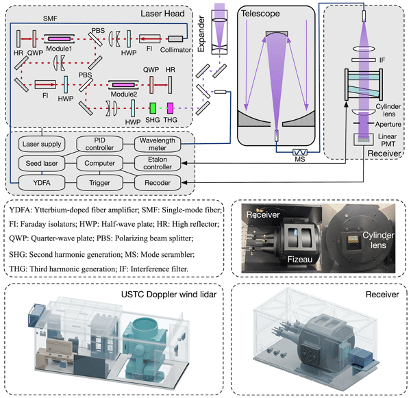
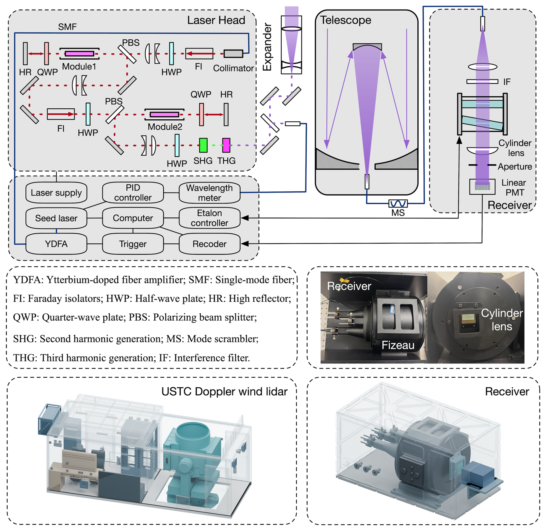
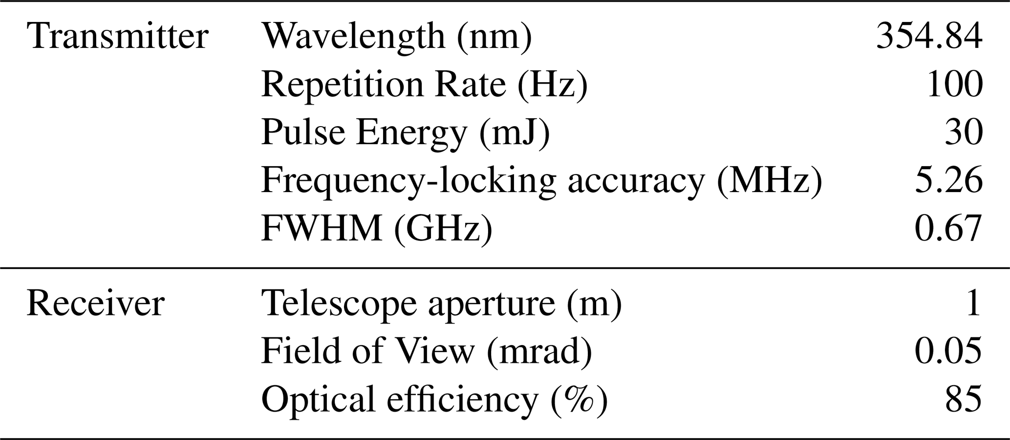
The schematic of the developed HSRL system is shown in Fig. 2. Except for the newly designed receiver, the overall lidar configuration is based on the USTC Doppler wind lidar system. The transmitter employs a fully solid-state, injection-seeded Nd:YAG master oscillator power amplifier (MOPA) system. A narrow-linewidth continuous-wave seed laser (NKT Photonics, K8230), operating at 1064 nm, serves as the initial optical source to provide a stable frequency reference. The seed beam is first amplified by a ytterbium-doped fiber amplifier (YDFA; Keopsys, PYFL-E02-LP-015-005-001-1064-G2-T1-ETO-PY9D-FA) and subsequently injected into a diode-pumped Nd:YAG laser head (Lumibird, 240794701), where it undergoes two stages of optical amplification to generate high-energy 1064 nm laser pulses. The amplified fundamental beam is then frequency converted through second-harmonic generation (SHG) and third-harmonic generation (THG), producing ultraviolet laser pulses at 355 nm. The final laser output has a pulse energy of 30 mJ at a repetition rate of 100 Hz. The laser beam is expanded by a beam expander before being transmitted into the atmosphere through a biaxial optical path. A small fraction of the transmitted 355 nm beam is directed into a wavelength meter (HighFinesse, WS8-2). The measured wavelength is fed to a custom-built PID controller, which stabilizes the transmitted laser frequency through feedback control of the 1064 nm seed laser. This reference channel ensures stable laser wavelength during long-term operation. After interacting with atmospheric molecules and aerosols, the backscattered light is collected by a Cassegrain telescope with a primary mirror diameter of 1 m. The received signal is coupled into a multimode optical fiber with a core diameter of 200 µm and a numerical aperture (NA) of 0.22, passed through a mode scrambler (MS) to improve the spatial uniformity of the output beam, and then delivered to the receiver. Within the receiver, the output beam from the optical fiber is first collimated and passes through a narrowband interference filter (IF) to suppress background radiation. The filtered signal is subsequently analyzed by a Fizeau interferometer, which converts the Doppler-shifted Rayleigh–Brillouin spectrum into a spatial interference fringe. Finally, the interference fringes emerging from the Fizeau interferometer are shaped by an aperture and then focused by a cylindrical lens onto a linear PMT. The acquired photon-counting data are transmitted to the computer for subsequent wind and temperature retrieval. The main parameters of the HSRL system are summarized in Table 1.

Figure 2 Schematic of the developed HSRL system.

Table 1 The basic parameters of lidar system.

The basic parameters of the Fizeau interferometer should be determined by RB spectrum. Under the small-wedge-angle condition, its transmission can be approximated by the Airy function (McKay, 2002; Vaughan et al., 2025). When the finite divergence of the incident beam is considered, the Airy function is averaged over the angular distribution, yielding the transmission function given in Eq. (10).

$$\begin{array}{}\text{(10)}& F\left(\mathit{\nu }\right)={\displaystyle \frac{\mathrm{2}}{{\mathit{\theta }}_{\mathrm{0}}^{\mathrm{2}}}}\underset{\mathrm{0}}{\overset{{\mathit{\theta }}_{\mathrm{0}}}{\int }}{T}_{\mathrm{p}}\sin \mathit{\theta }{\left[\mathrm{1}+{\displaystyle \frac{\mathrm{4}{F_R}^{\mathrm{2}}}{{\mathit{\pi }}^{\mathrm{2}}}}\sin {\left({\displaystyle \frac{\mathit{\pi }\mathit{\nu }\cos \mathit{\theta }}{\mathrm{FSR}}}\right)}^{\mathrm{2}}\right]}^{-\mathrm{1}}\mathrm{d}\mathit{\theta },\end{array}$$

where T_p is the peak transmittance of the interferometer, θ₀ is the divergence angle of the incident light in the Fizeau interferometer, θ is the angle of incidence in the Fizeau interferometer, ν is the frequency, and FSR is the free spectral range of the interferometer. The selection of FSR must ensure that it is greater than the width of the molecular scattering spectrum within the detection range, and not more than twice the bandwidth at 10 % of the RB line peak. Therefore, the FSR of the Fizeau interferometer should be within the range of 10 to 12.6 GHz. Based on this requirement, an existing tunable etalon (ET116FS-1068) can be modified to function as a Fizeau interferometer. The parameters of the Fizeau interferometer are summarized in Table 2.

Table 2 Parameters of the Fizeau interferometer.

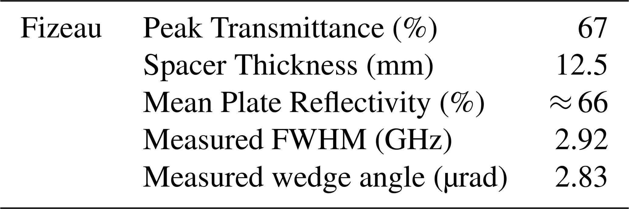
3.2 Simulation-based parameter optimization

The number of channels in the linear PMT array and the wedge angle of the Fizeau interferometer are key parameters that need to be optimized according to the existing instrument configuration. Therefore, simulations are performed to evaluate the performance of the proposed receiver and determine the optimal values of these parameters.

To ensure that the convolution of the RB spectrum and the transmittance of the Fizeau interferometer can be fully captured by the linear PMT, the frequency range of the linear PMT captured can be designed to be twice the bandwidth of the RB spectrum. Based on this, the wedge angle of the Fizeau interferometer can be calculated using Eq. (11):

$$\begin{array}{}\text{(11)}& \mathit{\alpha }=\arctan \left({\displaystyle \frac{\mathrm{2}{L}_{\mathrm{0}}\mathrm{\Delta }{\mathit{\nu }}_{\mathrm{RB}}}{L_{\mathrm{if}}{\mathit{\nu }}_{\mathrm{0}}}}\right),\end{array}$$

where L_if is the target area width of the linear PMT, L₀ is the central cavity length of the Fizeau interferometer, Δν_RB is the RB spectral line width, and ν₀ is the laser frequency. Taking Δν_RB as the RB spectral line bandwidth at 10 km, the PMT target area width is determined by the number of channels, after optimizing the number of channels as described below, the ideal wedge angle α can be obtained.

For a laser pulse emitted by a lidar, the number of photons received at a distance z is given by the lidar equation in Eq. (12):

$$\begin{array}{}\text{(12)}& N\left(z\right)={\displaystyle \frac{E_{\mathrm{0}}}{h{\mathit{\nu }}_{\mathrm{laser}}}}{\displaystyle \frac{A_{\mathrm{r}}}{z^{\mathrm{2}}}}{\mathit{\eta }}_{\mathrm{q}}{\mathit{\eta }}_{\mathrm{o}}\mathit{\beta }\left(z\right)\exp \left[-\mathrm{2}\underset{\mathrm{0}}{\overset{z}{\int }}\mathit{\alpha }\left(z\right)\mathrm{d}z\right]\mathrm{\Delta }z,\end{array}$$

where E₀ is the energy of a single laser pulse; h is Planck's constant; η_q is the quantum efficiency of the detector; η_o is the optical system efficiency; ν_laser is the laser emission frequency; Δz is the lidar range resolution; A_r is the effective receiving area of the receiving telescope; β(z) is the sum of the backscattering coefficients of aerosols and atmospheric molecules at detection distance z; α(z) is the sum of the aerosol and atmospheric molecular extinction coefficients at a distance z.

Under ideal conditions, the incident illumination is assumed to be spatially uniform, all light emerging from the Fizeau interferometer is imaged onto the linear PMT array by the cylindrical lens, and all PMT channels have identical detection responses. The expected photon count in each channel is then obtained by integrating the convolved spectral response over the channel width and multiplying by $N\left(z\right)/L_{\mathrm{if}}$, as shown in Eq. (13):

$$\begin{array}{}\text{(13)}& \begin{array}{rl}& N_j\left(y_j,\mathit{\nu },z,T\right)=\\ & {\displaystyle \frac{N\left(z\right)}{L_{\mathrm{if}}}}\cdot \underset{y_j-\mathrm{\Delta }y/\mathrm{2}}{\overset{y_j+\mathrm{\Delta }y/\mathrm{2}}{\int }}\left\{\left[S_{\mathrm{rb}}\left(\mathit{\nu },z,T\right)+S_{\mathrm{Mie}}\left(\mathit{\nu }\right)\right]\right.\\ & \left.\otimes F\left(\mathit{\nu }-\mathit{\nu }\left(y\right)\right)\otimes S_{\mathrm{laser}}\left(\mathit{\nu }\right)\right\}\mathrm{d}y,\end{array}\end{array}$$

where y_j represents the center coordinate of the jth channel of the linear PMT, where $y_j=(j+\mathrm{0.5}-n_{\mathrm{channel}}/\mathrm{2})\cdot {\mathrm{pitch}}_{\mathrm{Array}}$, and pitch_Array is the distance between the centers of two adjacent detection units in the array PMT; Δy is the effective width of each detector channel; v(y) maps spatial coordinates to frequency coordinates, where $v\left(y\right)=(y\cdot \mathrm{2}\mathrm{\Delta }{\mathit{\nu }}_{\mathrm{RB}})/L_{\mathrm{if}}$; S_Mie(ν) is the Mie scattering spectrum which is represented by a delta function. The combined spectrum S_rb+S_Mie is normalized to unit area. Thus, for the jth channel, the total expected counts can be expressed as: $N_{\mathrm{total}}=N_j+N_{\mathrm{d}}+N_{\mathrm{b}}$, where N_d is the expected dark noise produced by the detector and N_b is the expected background noise. In conditions that the backscattering signal received with this lidar system is weak, the number of photons is not sufficiently high. Accordingly, the statistical distribution of N_total satisfies the Poisson distribution, as shown in Eq. (14):

$$\begin{array}{}\text{(14)}& P(x=n)=P_n=e^{-\mathit{\lambda }}{\displaystyle \frac{{\mathit{\lambda }}^n}{n\mathrm{!}}}.\end{array}$$

Previous studies have investigated the influence of spectral sampling on parameter estimation accuracy. Hagen et al. (2007) examined the effects of sampling density, finite pixel width, and noise on the estimation of Gaussian spectral parameters, highlighting the importance of balancing spectral sampling resolution and measurement uncertainty (Hagen et al., 2007). In the present study, our retrieval method involves four free parameters, requiring at least four spectrally independent measurements as a necessary, but not sufficient, condition for local parameter identifiability. To evaluate the influence of spectral sampling density on retrieval performance, numerical simulations were conducted using seven detector configurations with 4, 8, 16, 32, 64, 128, and 256 channels.

The signals were simulated using a Monte Carlo method based on the 1976 U.S. Standard Atmosphere over a height range of 2–30 km, with vertical resolutions of 60 m below 10 km and 300 m at and above 10 km. For each detector configuration, 1000 independent Monte Carlo simulations were performed. In each simulation, multichannel photon-counting signals were generated and fitted to retrieve temperature and wind velocity, with retrieval accuracy evaluated using the root-mean-square error (RMSE). This approach provides a direct assessment of the influence of detector channel number on the accuracy of temperature and wind retrievals under different signal-to-noise conditions.

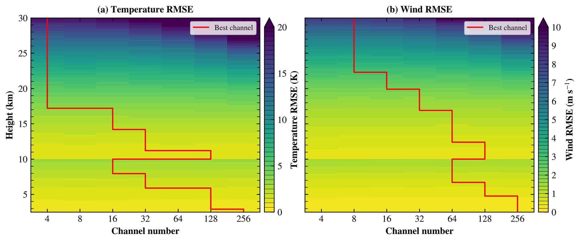
Figure 3 Influence of detector channel number and detection height on the retrieval accuracy of (a) temperature and (b) wind velocity. The color bars indicate the corresponding RMSEs. The red line indicates the optimal number of detector channels for different detection altitudes.

As shown in Fig. 3a, in regions with relatively high SNRs, increasing the number of detector channels provides only limited improvement in temperature retrieval accuracy. However, in regions with low SNRs, configurations with larger numbers of channels tend to exhibit higher temperature RMSEs. However, selecting too few channels may compromise the robustness of the retrieval system. Therefore, considering the trade-offs among retrieval robustness, system complexity, and the commercial availability of multichannel PMT arrays, a 32-channel linear PMT array (H11460-200, Hamamatsu) was selected for the proposed receiver. According to Eq. (11), the optimized wedge angle is 3.11 µrad, while the experimentally adjusted value is 2.83 µrad. The corresponding shape factor is S=0.062, well below 0.6, supporting the use of the Airy function.

4 Retrieval algorithm

To achieve more accurate simultaneous retrieval of atmospheric wind and temperature from the measured backscatter spectrum, an iterative retrieval algorithm based on nonlinear least-squares optimization is employed. The measured spectrum is fitted using the spectral model given in Eq. (15).

$$\begin{array}{}\text{(15)}& \begin{array}{rl}{N}_{\mathrm{fit}}\left(\mathit{\nu },z,T\right)=& \left(I_{\mathrm{RB}}\cdot S_{\mathrm{rb}}\left(\mathit{\nu },z,T\right)+I_{\mathrm{Mie}}\cdot S_{\mathrm{Mie}}\left(\mathit{\nu }\right)\right)\\ & \otimes F\left(\mathit{\nu }\right)\otimes S_{\mathrm{laser}}\left(\mathit{\nu }\right),\end{array}\end{array}$$

The fitting yields four parameters: the RB scattering intensity I_RB, the Mie scattering intensity I_Mie, the frequency shift ν, and the atmospheric temperature T. The overall procedure of the proposed joint retrieval algorithm is illustrated in Fig. 4.

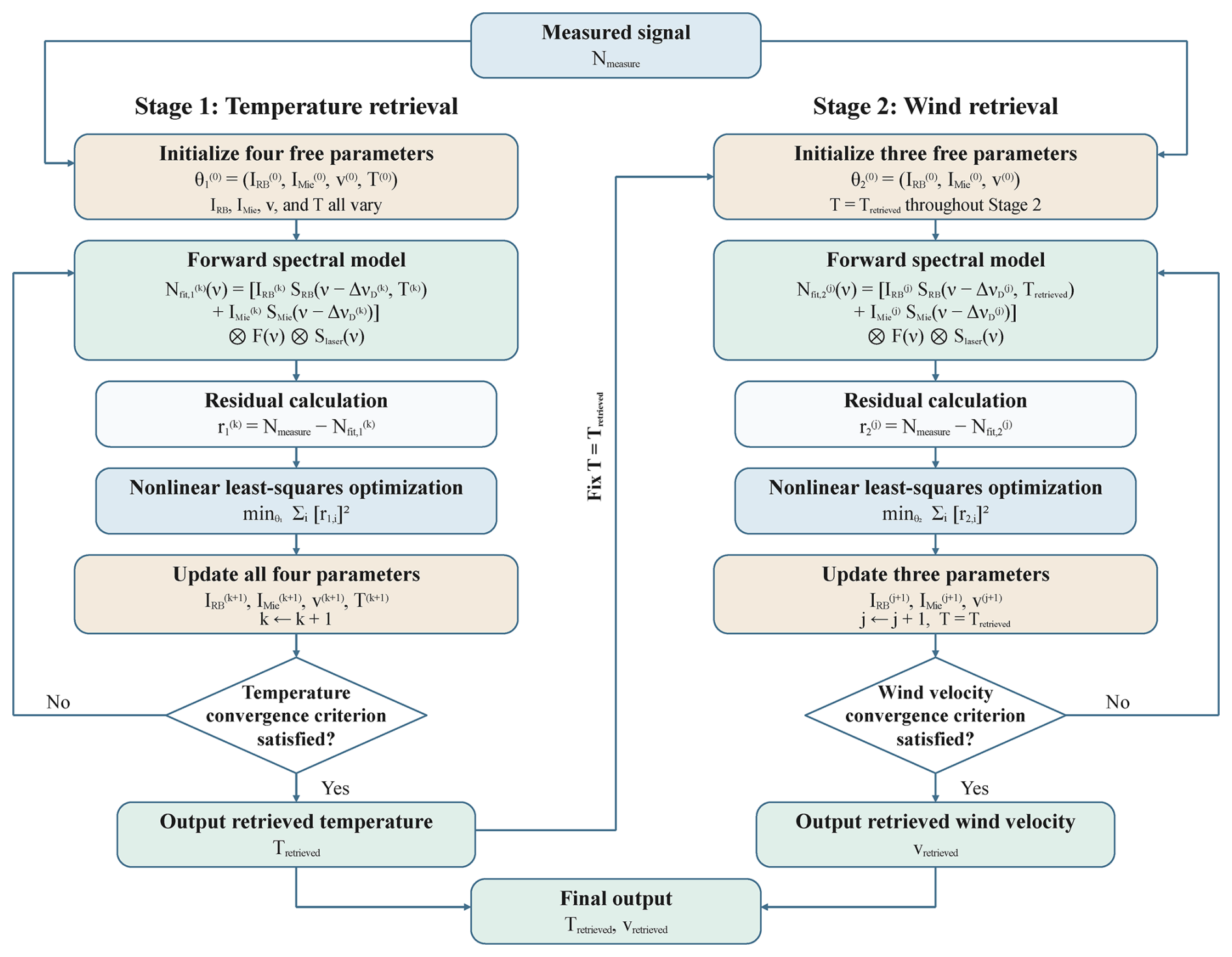
Figure 4 Flowchart of the iterative retrieval algorithm for simultaneous atmospheric wind and temperature retrieval based on nonlinear least-squares optimization.

To further evaluate the selected 32-channel configuration and the retrieval algorithm, 100 independent Monte Carlo simulations were performed at each altitude. Temperature and wind velocity were retrieved using Eq. (15) with both small (temperature: +5 K; wind velocity: +5 m s⁻¹; RB amplitude: +20 %; Mie amplitude: −20 %) and large (temperature: +20 K; wind velocity: +20 m s⁻¹; RB amplitude: +50 %; Mie amplitude: −50 %) initial-guess deviations to assess the number of iterations required for convergence under different initialization conditions.

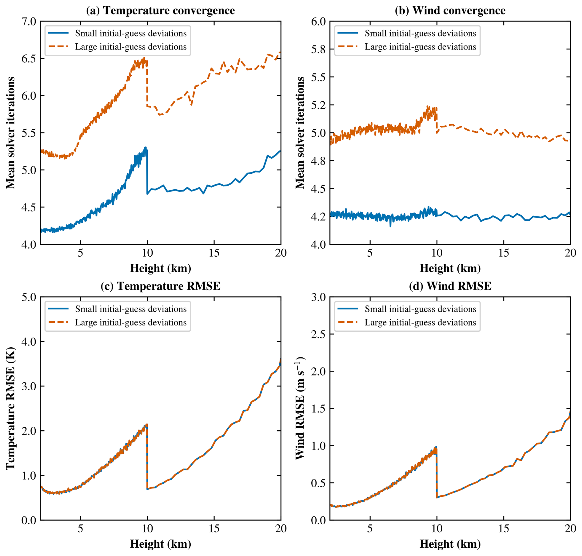
Figure 5 Comparison of mean solver iteration counts for (a) temperature and (b) wind velocity retrievals, and RMSEs of (c) temperature and (d) wind velocity. Blue solid and orange dashed lines represent small and large initial-guess deviations in all four parameters, respectively.

As shown in Fig. 5a and b, temperature retrieval requires approximately 4–5 iterations for small initial-guess deviations and 5–7 iterations for large deviations, whereas wind velocity retrieval requires approximately 4 and 5 iterations, respectively. The iteration count for temperature retrieval generally increases with altitude within each vertical resolution interval, while that for wind velocity retrieval remains relatively stable. Despite these differences in convergence behavior, the temperature and wind velocity RMSE curves for the two levels of initial-guess deviations nearly overlap, as shown in Fig. 5c and d, indicating that the final retrieval accuracy is largely insensitive to the initial-guess deviations tested.

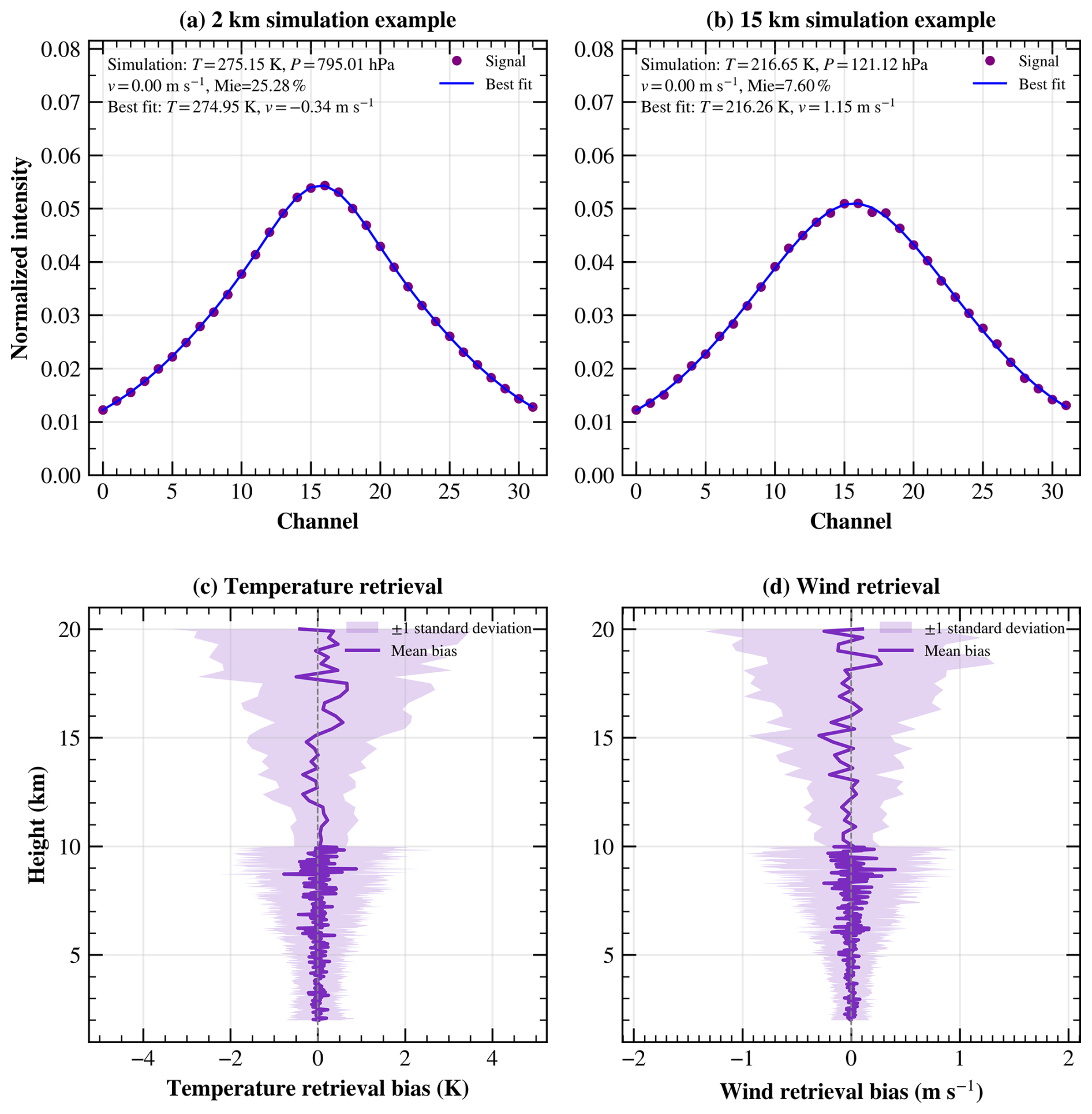
Figure 6 Examples of normalized simulated photon counts and their best fits at (a) 2 km and (b) 15 km. Mean retrieval biases and standard deviations of (c) temperature and (d) wind velocity as functions of height.

The retrieval accuracy of the receiver design and the joint retrieval algorithm is further evaluated in Fig. 6. Figure 6a and b show the simulated signals and their best fits for the first Monte Carlo realization at 2 and 15 km, respectively. Figure 6c and d present the mean temperature and wind velocity retrieval biases across 100 Monte Carlo realizations, with shaded bands indicating ±1 standard deviation.

As shown in Fig. 6c and d, the mean temperature and wind velocity retrieval biases remain close to zero across most heights. Across all simulated heights and realizations, the mean biases are 0.02 K and −0.003 m s⁻¹, and the corresponding mean absolute errors (MAEs) are 1.5 K and 0.6 m s⁻¹, respectively. The standard deviations increase overall from 0.6 K and 0.2 m s⁻¹ at 2 km to 2.9 K and 1.3 m s⁻¹ at 20 km. Field experiments are needed to further validate the performance of the proposed system and retrieval algorithm under actual atmospheric conditions.

5 Experiments

5.1 Calibration

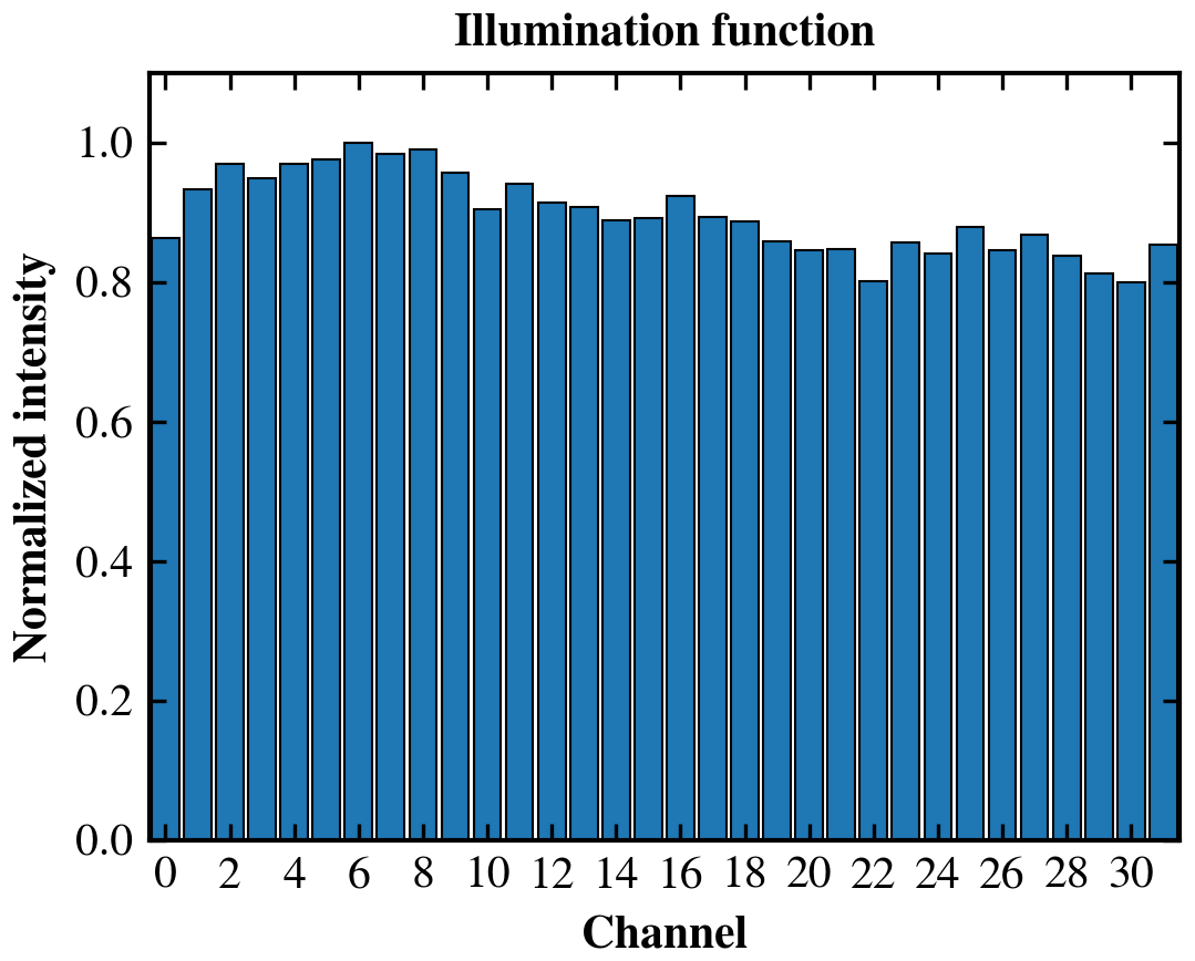
The response nonuniformity among the individual channels of the 32-channel PMT array can directly affect the measured spectral distribution and consequently introduce errors into the spectral retrieval. Therefore, the illumination function of the receiver was independently characterized and corrected. The illumination function was calibrated using a broadband LED light source by normalizing the intensity distribution measured by the 32-channel PMT array, which was subsequently used to correct the measured spectra.

Figure 7 shows the illumination, which was adopted for the correction of the measured spectra. For each measurement, the photon counts recorded by each PMT channel were corrected by multiplying them by the reciprocal of the corresponding illumination-function value.

Figure 7 Illumination function of the 32-channel PMT array.

To experimentally validate the proposed receiver design, an HSRL receiver was constructed using the parameters described above. To ensure measurement accuracy, the receiver transmission function was characterized using a 355 nm continuous-wave laser in the laboratory and the 355 nm pulsed laser of the USTC Doppler wind lidar under actual operating conditions. The pulsed-laser measurements were performed directly on the experimental lidar system. Furthermore, the optical fiber and mode scrambler used during the calibration measurements were identical to those employed during the atmospheric measurements, ensuring consistent optical illumination conditions between calibration and field measurements. The results are shown in Fig. 8.

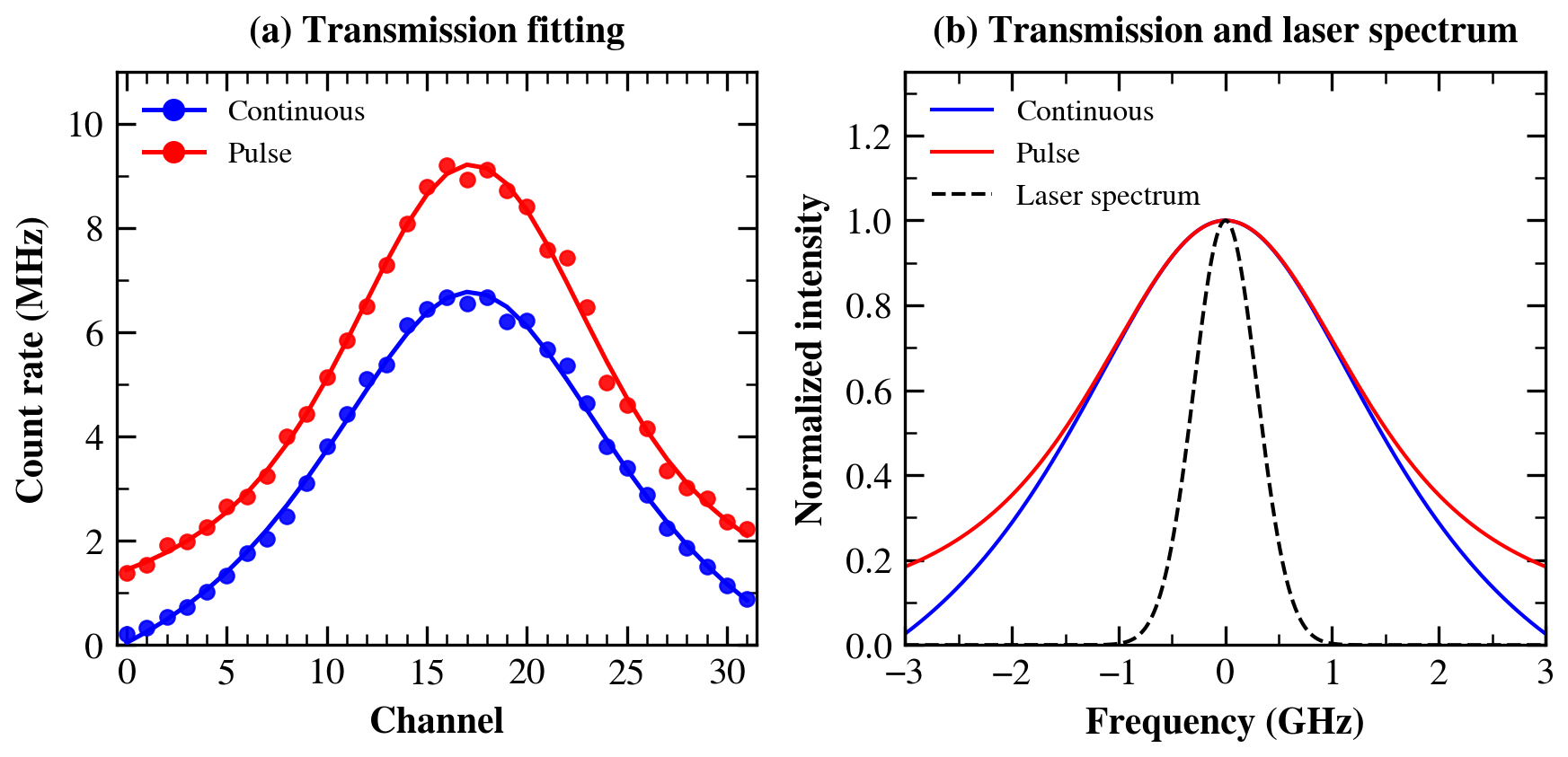
Figure 8 Receiver calibration results. (a) Receiver transmittance measured with a continuous-wave laser (blue circles) and a pulsed laser (red circles), together with their corresponding fitted curves. (b) Retrieved transmission functions for the continuous-wave and pulsed-laser measurements and the deconvolved Gaussian laser spectrum (black dashed line).

As shown in Fig. 8a, the transmission response measured using the continuous-wave laser was fitted with an Airy function, whereas the response measured using the pulsed laser was fitted by convolving the Airy function with a Gaussian function representing the laser spectrum. As shown in Fig. 8b, deconvolution of the continuous-wave and pulsed-laser responses yields the pulsed-laser spectrum, with a retrieved linewidth of 0.67 GHz.

To calibrate the receiver response to Doppler frequency shifts, frequency-scanning measurements were performed using a tunable continuous-wave laser. The laser frequency was varied over a known range, while the corresponding displacement of the interference fringe on the 32-channel PMT array was recorded. This procedure establishes the relationship between the optical frequency shift and the channel displacement, which is subsequently used to convert the measured fringe displacement into a Doppler frequency shift. During atmospheric measurements, the fringe peak is primarily located within and shifts among the central channels of the detector. Therefore, the calibration measurements were focused mainly on this region. A total of six independent frequency-scanning measurements were performed. One measurement covered the full response range of the 32-channel detector to characterize the overall frequency-to-channel relationship, whereas the other five measurements were restricted to the central six channels, corresponding to the region relevant to the atmospheric Doppler measurements. The calibration results are shown in Fig. 9.

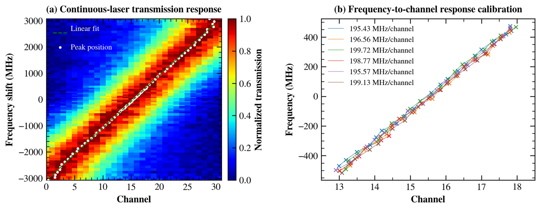
Figure 9 Calibration of the frequency-to-channel response. (a) Measured continuous-wave laser transmission response as a function of detector channel and laser frequency shift. The white dots indicate the fitted peak positions, and the dashed line represents the corresponding linear fit. (b) Frequency-to-channel response obtained from six independent frequency-scanning measurements, with the fitted slopes indicated in the legend.

As shown in Fig. 9a, the frequency-to-channel response was first characterized over the full range of the 32-channel detector. A nearly linear relationship between the laser frequency shift and the fitted peak position was observed over most of the detector range. Some deviations from linearity occur near the edges of the detector (around channels 0 and 31), which are mainly attributed to variations in the output energy of the tunable laser during the frequency scan and the limited spectral information available when the transmission peak approaches the edge of the detector. For wind retrieval, however, the spectral peak is primarily located within the central six channels, corresponding approximately to a Doppler-frequency-shift range of −500 to 500 MHz. Therefore, the full-range scan and five additional scans near the central channels were used to characterize the frequency-to-channel response in this effective working region, as shown in Fig. 9b. The resulting mean response was 197.53 MHz per channel, with a standard deviation of 1.90 MHz per channel, and this value was used for the subsequent Doppler-frequency-shift and wind retrievals.

5.2 Effect of Mie scattering on temperature retrieval

To evaluate the effect of Mie scattering on temperature retrieval, measurements were performed using the USTC Doppler wind lidar in Xinjiang, China, at 14:00 UTC. The telescope was oriented vertically with a total integration time of 5 min. The vertical resolution was 60 m below 10 km and 300 m above 10 km. By fitting the raw experimental data, the RB and Mie spectra can be separated, and the atmospheric temperature can be retrieved. The retrieved temperature, together with the relative RB and Mie scattering intensities, can subsequently be used to assess the influence of Mie scattering on the temperature retrieval.

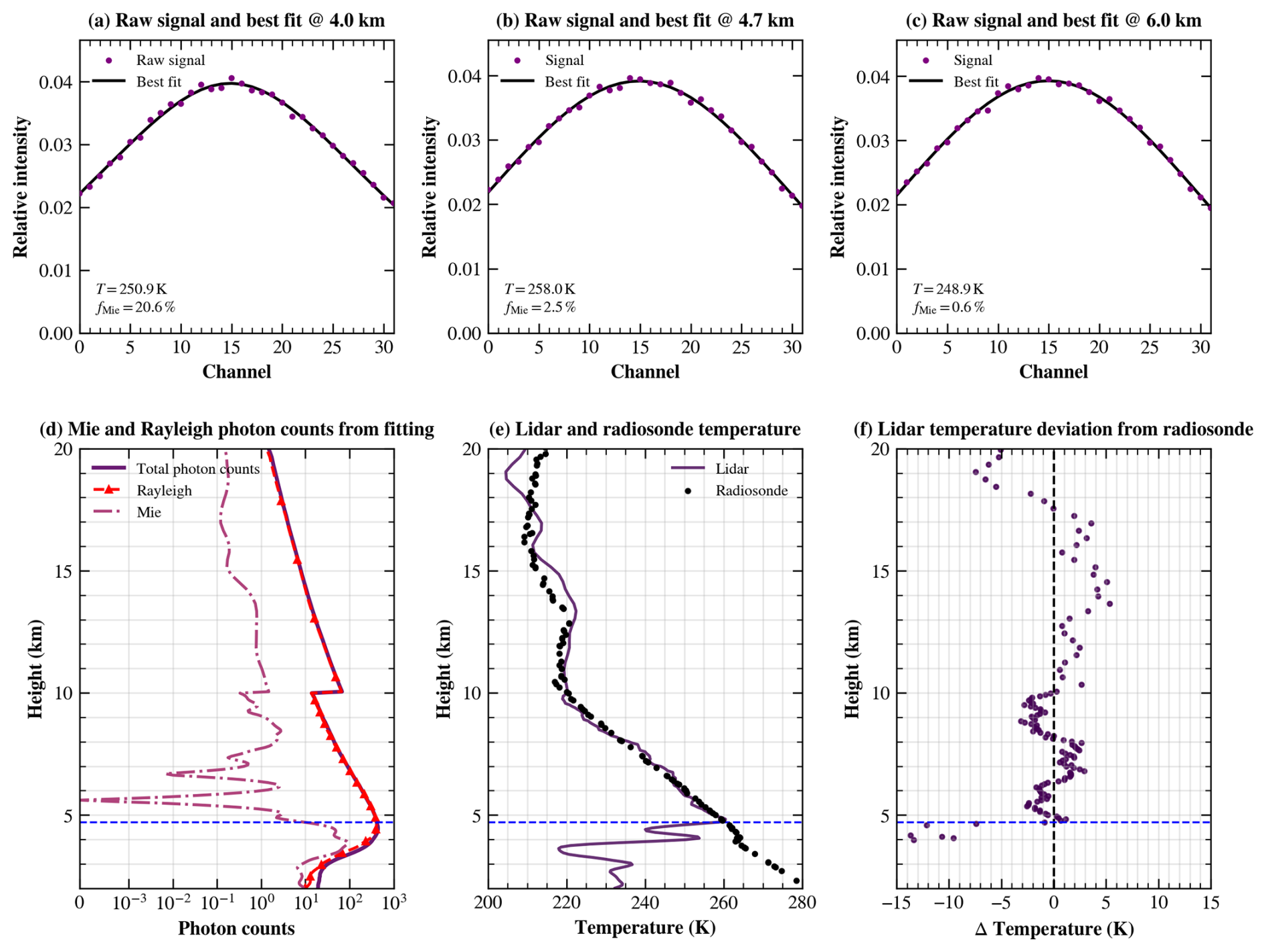
Figure 10 Spectral fitting results and evaluation of the influence of Mie scattering on temperature retrieval. (a–c) Best-fitting results of the measured signals at 4.0, 4.7, and 6.0 km. (d) Retrieved total, RB, and Mie photon counts. (e) Comparison between the lidar-retrieved and radiosonde temperature profiles. (f) Temperature difference (lidar minus radiosonde). The blue dashed line indicates the lower boundary of the temperature retrieval (4.7 km).

As shown in Fig. 10, the Mie scattering signal decreases rapidly above 4.0 km. By analysing the relationship between the Mie scattering signal fraction and the temperature retrieval difference relative to the radiosonde measurements, the lower boundary for reliable temperature retrieval was determined. Strong Mie scattering below 4.7 km significantly affects the accuracy of temperature retrieval. Therefore, temperature retrieval is performed only where the Mie scattering signal fraction is below 8 %. The lower boundary for temperature retrieval is therefore not fixed but depends on the aerosol and cloud conditions during each observation. For the measurement shown in Fig. 10, this criterion corresponds to an altitude of approximately 4.7 km. For the height range from the onset of telescope–laser overlap to the temperature retrieval boundary, wind retrieval is carried out using model-derived temperature as the input.

5.3 Simultaneous measurement of temperature and wind speed

Measurements were performed using the USTC Doppler wind lidar in Xinjiang, China (43.8° N, 87.6° E), at 20:00 UTC under conditions with thin clouds near 5 km. During the measurements, the telescope was tilted by 15° from the vertical and sequentially pointed toward the east, west, south, and north, with an integration time of 5 min in each direction. For ease of interpretation, the measured spectra at each altitude were normalized to unit area. The resulting spectra, covering the altitude range from 2 to 20 km, have a temporal resolution of 5 min and vertical resolutions of 60 m below 10 km and 300 m above 10 km, as shown in Fig. 11.

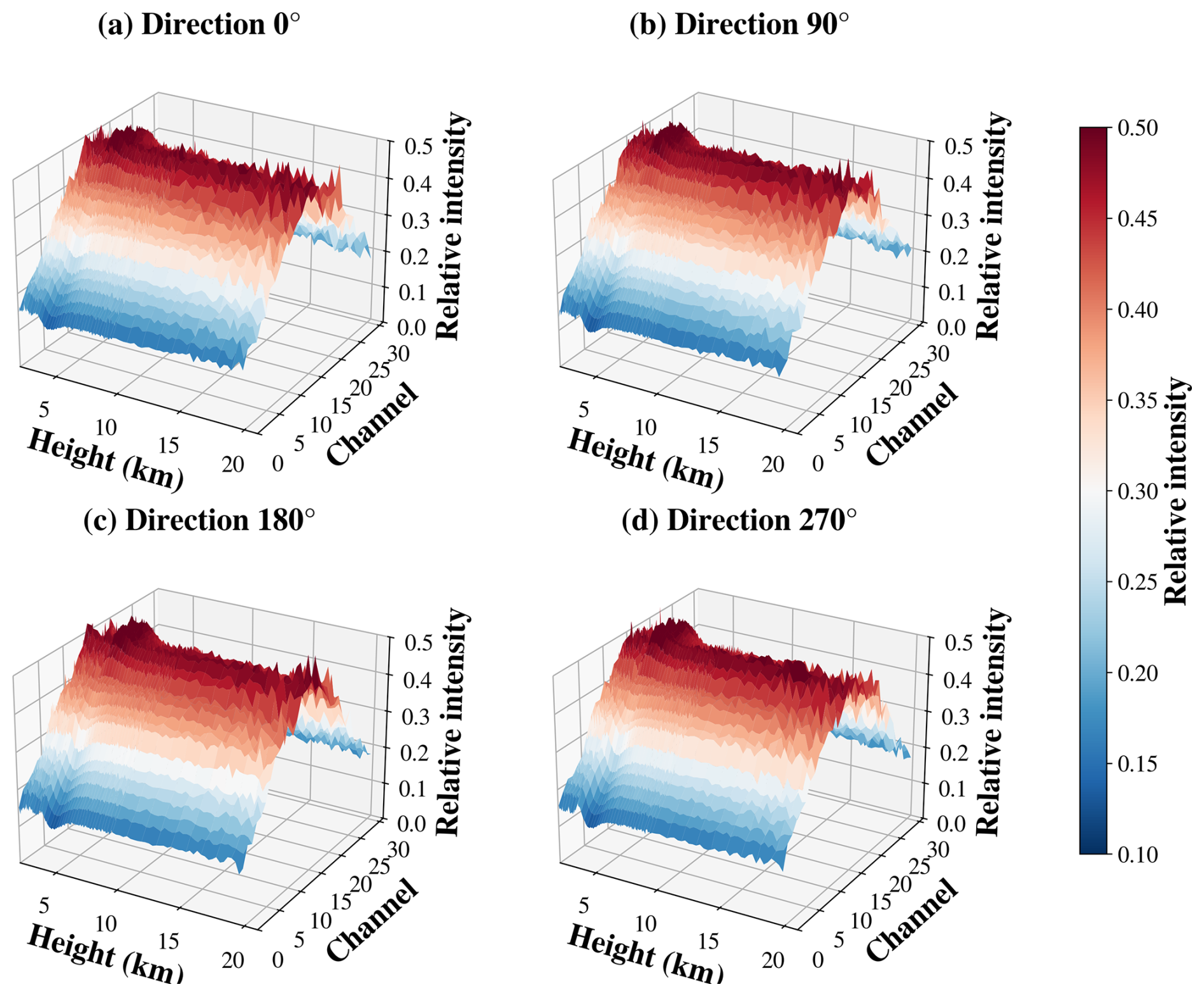
Figure 11 Spectra measured in four directions ranging from 2 to 20 km and normalized to unit area.

Figure 11 shows the raw data measured by the HSRL system. Because the system uses an off-axis design, signals below 2 km are outside the telescope field of view; therefore, the measurements start at 2 km. The atmospheric scattering spectrum measured near 5 km is significantly influenced by thin clouds, which effectively narrows the observed spectral profile and degrades the accuracy of molecular spectral retrieval. Therefore, based on the Mie-contamination threshold determined above, temperature retrievals are performed only above 5.3 km. The temperature and wind profiles retrieved from the spectral data shown in Fig. 11 are presented in Figs. 12 and 13, respectively, together with their deviations from the radiosonde measurements. The radiosonde launch site was located approximately 100 km from the lidar observation site.

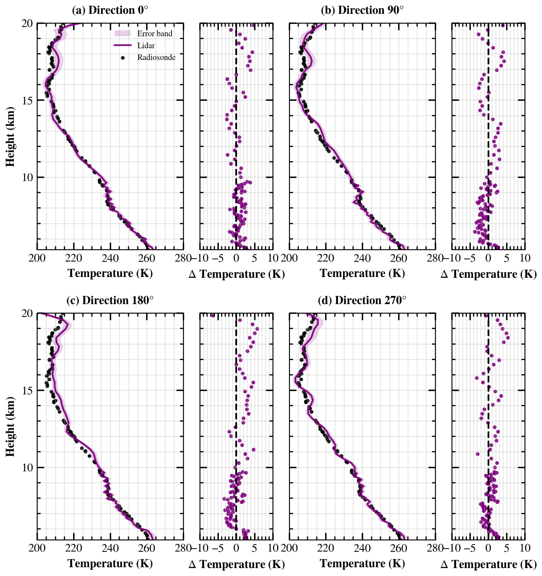
Figure 12 Temperature profiles retrieved from the lidar measurements in four directions (purple lines), together with the radiosonde temperature profile (black dots) and the corresponding temperature differences.

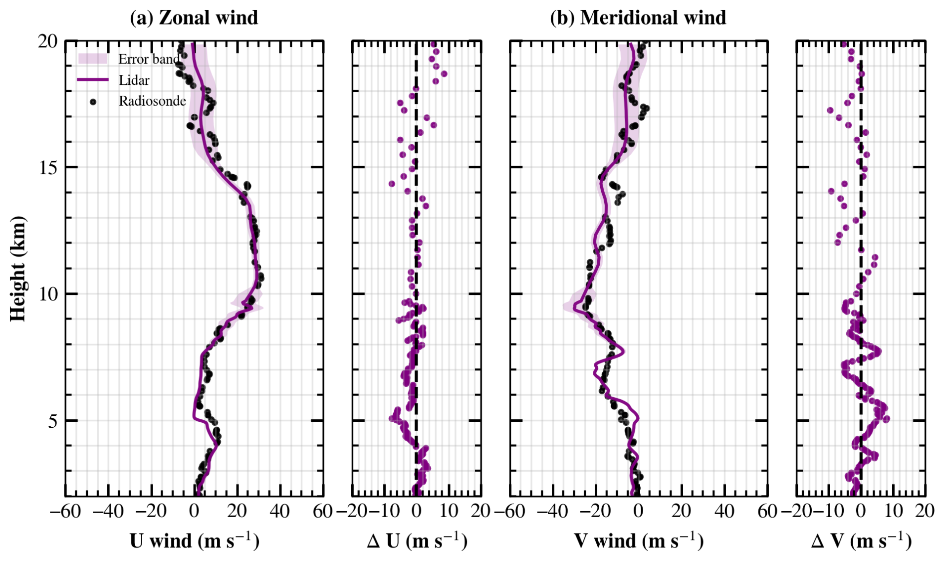
Figure 13 Retrieved zonal and meridional wind profiles (purple lines), together with the radiosonde measurements (black dots) and the corresponding wind differences.

As shown in Fig. 12, the purple lines represent the temperature profiles retrieved from the lidar measurements, while the black dots represent the radiosonde temperature profile. The error bands indicate the fitting uncertainty, which ranges from 1.55 to 2.02 K at a range resolution of 60 m and from 1.49 to 3.04 K at a range resolution of 300 m. Compared with the radiosonde measurements, the retrieved temperatures showed absolute differences of less than 3.70 K, with a mean absolute difference of 1.19 K at a range resolution of 60 m. Above 10 km, where the range resolution was increased to 300 m, the absolute differences remained below 6.35 K, with a mean absolute difference of 2.10 K.

For wind retrieval, the laser frequency was continuously monitored by a wavelength meter during the atmospheric measurements, providing a real-time frequency reference for the Doppler shift determination. Below 5.3 km, the fitting was performed using model-provided temperatures, whereas above 5.3 km, wind velocity and temperature were retrieved simultaneously. To further reduce systematic frequency offsets, the line-of-sight wind velocities measured in opposite azimuth directions were combined through differential processing before calculating the zonal and meridional wind components, as illustrated in Fig. 13.

The fitting uncertainty of the retrieved zonal and meridional wind components ranged from 0.47 to 1.19 m s⁻¹ below 5.3 km, from 0.63 to 5.98 m s⁻¹ between 5.3 and 10 km, and from 1.57 to 6.31 m s⁻¹ above 10 km. In the altitude range from 2.0 to 5.3 km, where temperature constraints were applied to the wind retrieval, the retrieved horizontal winds were generally consistent with the radiosonde measurements. The zonal wind showed a mean absolute difference of 2.34 m s⁻¹, with absolute differences of less than 7.44 m s⁻¹, while the meridional wind showed a mean absolute difference of 2.50 m s⁻¹, with absolute differences of less than 7.66 m s⁻¹. Between 5.3 and 10 km, where a range resolution of 60 m was used, the zonal and meridional winds showed absolute differences of less than 6.13 and 6.74 m s⁻¹, respectively, with corresponding mean absolute differences of 1.84 and 2.97 m s⁻¹. Some discrepancies are observed below 10 km, particularly around 5 km. Considering that the radiosonde launch site was located approximately 100 km from the lidar observation site, these discrepancies may partly be attributed to the spatial inhomogeneity of the tropospheric wind field, as the two measurements sampled different air masses. Above 10 km, where the range resolution was increased to 300 m, the zonal and meridional winds showed absolute differences of less than 8.65 and 8.78 m s⁻¹, respectively, with corresponding mean absolute differences of 3.02 and 3.08 m s⁻¹.

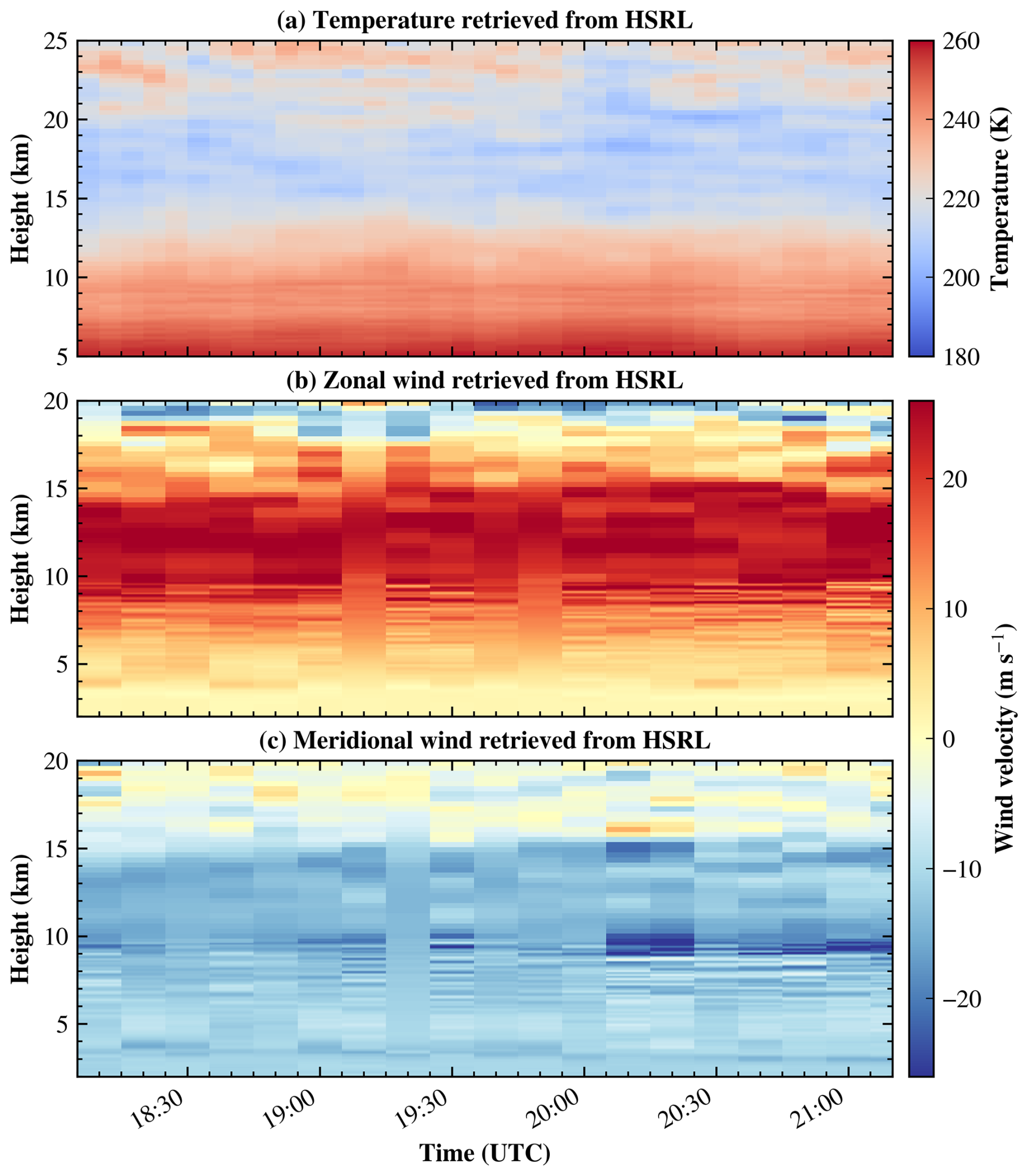
Figure 14 Time–height distributions of the retrieved temperature (a), zonal winds (b) and meridional winds (c).

Figure 14 presents continuous measurements obtained during a separate observation period. Based on the aerosol conditions during this measurement, the lower boundary for temperature retrieval was approximately 5 km. Simultaneous retrievals of wind and temperature were achieved from 5 to 20 km, whereas wind retrievals from 2 to 5 km were performed using model-provided temperature constraints. For a more comprehensive characterization of the vertical temperature structure, the temperature retrieval was extended to 25 km. The retrieved temperature profiles have a temporal resolution of 5 min. Because the telescope sequentially scans different azimuth directions, wind retrieval requires measurements from two consecutive scan positions, resulting in a temporal resolution of 10 min.

As shown in Fig. 14, the temporal stability of the continuous observations was evaluated using the standard deviation of the retrieved profiles. The standard deviation of the retrieved temperature ranged from 0.61 to 4.83 K over the altitude range of 5–20 km. The standard deviations of the retrieved meridional and zonal winds ranged from 0.15 to 8.56 m s⁻¹ and from 0.24 to 5.97 m s⁻¹, respectively. For both wind components, the largest standard deviations were observed between 9 and 15 km, corresponding to the altitude range of the westerly jet, where relatively strong winds and enhanced atmospheric variability resulted in larger temporal fluctuations.

6 Summary

In this study, we developed a Fizeau-interferometer-based HSRL receiver for simultaneous atmospheric wind and temperature measurements. By combining spectral-to-spatial conversion with a 32-channel linear PMT array, the complete atmospheric scattering spectrum can be recorded in a single measurement without frequency scanning, enabling simultaneous retrieval of atmospheric wind velocity and temperature through spectral fitting. This receiver architecture eliminates the need for frequency scanning while maintaining the capability to simultaneously retrieve both atmospheric parameters.

Simulation results demonstrated that the optimized 32-channel configuration provides an appropriate balance between spectral resolution and photon utilization over the 2–20 km altitude range. Field experiments further verified reliable wind retrievals from 2 to 20 km and simultaneous wind–temperature retrievals from 5.3 to 20 km, with good agreement with radiosonde observations, demonstrating the feasibility of simultaneous atmospheric wind and temperature measurements using a multichannel Fizeau interferometer without frequency scanning.

The results indicate that the retrieval performance is limited by different factors at different altitudes. In the lower troposphere, the received photon counts are sufficiently high, and the retrieval accuracy is mainly limited by the strong Mie scattering, which obscures the broad molecular RB spectrum and increases the difficulty of separating the molecular and aerosol scattering components. Under these conditions, increasing the spectral sampling density is more beneficial than further improving the SNR. Therefore, a Fizeau interferometer with a smaller wedge angle, combined with a detector having a larger number of channels, would provide finer spectral sampling of the atmospheric scattering spectrum, enabling more accurate reconstruction of spectral features and more reliable separation of the molecular and aerosol scattering components. This configuration reduces the frequency interval represented by each detector channel, allowing finer sampling of the atmospheric scattering spectrum.

In contrast, at higher altitudes the molecular backscatter signal decreases rapidly, and the retrieval uncertainty is primarily limited by photon noise rather than spectral sampling. Under these conditions, redistributing the received photons into fewer detector channels becomes more important than preserving fine spectral details. A Fizeau interferometer with a larger wedge angle compresses the atmospheric scattering spectrum into fewer detector channels, thereby increasing the photon counts per channel and improving the SNR. Although this results in a coarser spectral sampling, the enhanced photon utilization provides more robust spectral fitting and improves the retrieval precision of both atmospheric temperature and wind velocity under low-signal conditions.

These considerations suggest that an adaptive multichannel Fizeau receiver employing different wedge angles for different altitude ranges could provide a more optimal balance between spectral resolution and photon efficiency than a single fixed configuration. Such a receiver would exploit high spectral resolution in the lower atmosphere while maximizing photon utilization in the upper troposphere and lower stratosphere, thereby extending the measurement capability and improving the overall retrieval performance. In addition, the present receiver employs a PZT-tuned Fizeau interferometer, whose wedge angle is susceptible to long-term environmental variations and mechanical drift. Replacing the current design with a fixed-gap Fizeau interferometer would improve the long-term stability and robustness of the receiver, making it more suitable for continuous ground-based observations as well as future airborne and spaceborne Doppler lidar applications.

The proposed system provides a practical approach for simultaneous wind and temperature measurements in the troposphere and lower stratosphere and demonstrates the potential of multichannel Fizeau-based HSRL for future ground-based, airborne, and spaceborne atmospheric remote sensing.

Appendix A: Detailed simulation parameters and examples of raw data

The temperature, pressure, line-of-sight wind velocity, and Mie backscatter fraction profiles used in the simulations are shown in Fig. A1. The range resolution was 60 m below 10 km and 300 m above 10 km.

The first two of the 100 Monte Carlo realizations were selected as simulation examples, as shown in Fig. A2.

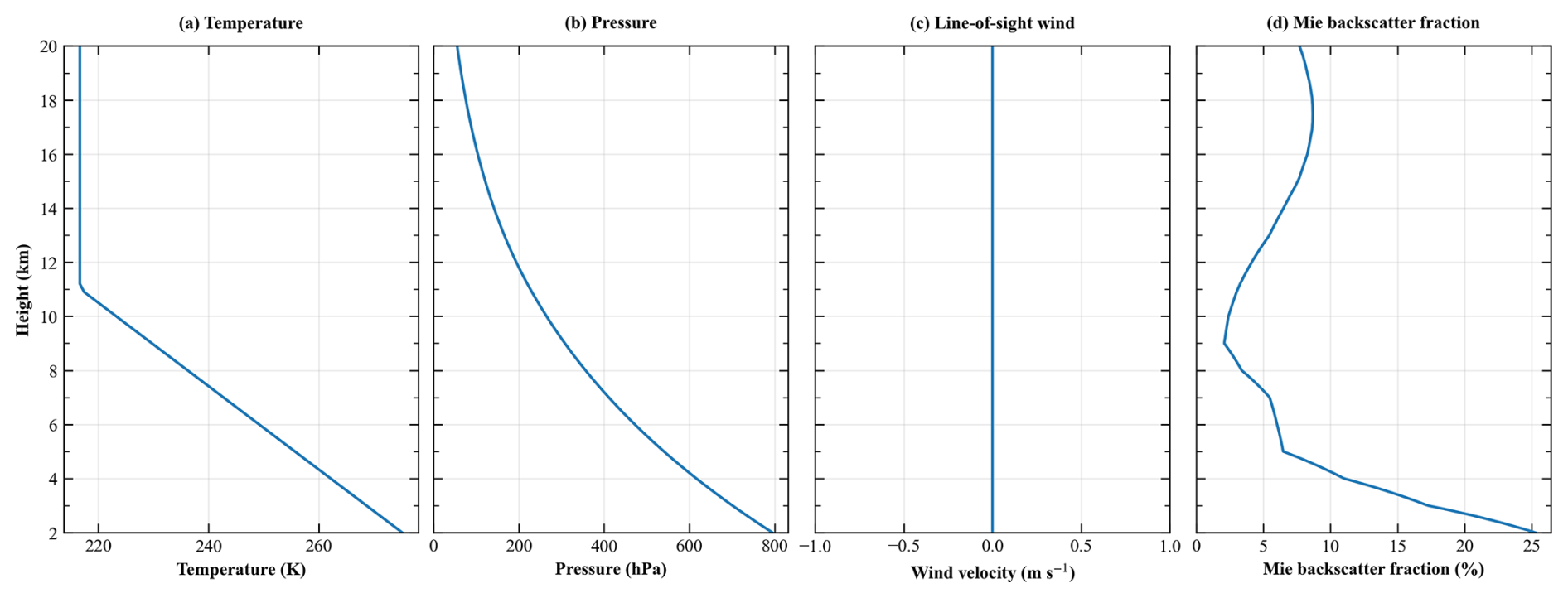
Figure A1 Profiles of (a) temperature, (b) pressure, (c) line-of-sight wind velocity, and (d) Mie backscatter fraction used in the simulations.

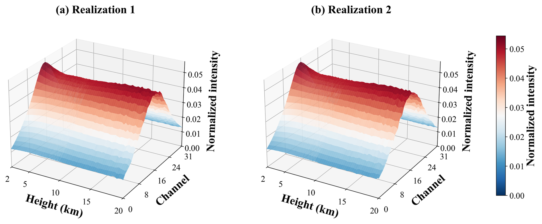
Figure A2 Simulated 32-channel photon counts for (a) the first and (b) the second Monte Carlo realizations.