
the Creative Commons Attribution 4.0 License.
the Creative Commons Attribution 4.0 License.
 | 19 Nov 2026
Machine-learning-based approach for solar radiation model prediction error identification, attribution and correction

Jorge Lezaca
Yves-Marie Saint-Drenan
Marion Schroedter-Homscheidt
Antti Arola
Accurate surface solar irradiance (SSI) is essential for climate monitoring and solar energy applications, yet operational radiation data products such as the Copernicus Atmosphere Monitoring Service (CAMS) solar radiation service (CRS) still exhibit systematic and situation dependent errors which are very specific due to CAMS internal parameterizations and retrieval implementation. These are arising from well-known uncertainties in clouds, aerosols and surface properties as well as from area-time mismatch between ground observations and pixel or model gridbox averaged properties, but error contributions of different parameters in various weather situations are not easy to quantify individually. In this study, we use two complementary families of data-driven XGBoost residual models for global horizontal (GHI), diffuse horizontal (DHI) and beam normal irradiance (BNI) using only the operational CRS inputs. Diagnostic models are interpreted using SHapley Additive exPlanations (SHAP) to characterise how the fitted models represent the residual structure in the analysed data, whereas separately tuned correction models are used to assess the generalisation performance of the post-process correction models. Across all components, cloud optical depth is identified as the primary feature associated with the radiation residuals represented by the diagnostic models. Aerosol and surface reflectance variables show additional component-dependent associations, particularly for DHI and BNI, but individual aerosol component rankings are interpreted as exploratory because the species-specific optical depths are correlated. The SHAP analysis also reveals a solar zenith angle dependence with contributions increasing at high solar zenith angles (SZA). Two single-case analyses under contrasting cloudy and aerosol-loaded conditions demonstrate how SHAP decomposes individual diagnostic-model residual predictions. We also apply the predictive models as a post-processing correction to CRS irradiance. On the test sets independent of training data, the correction reduces root mean squared error (RMSE) by 17.6 %, 20.5 %, and 23.9 % for GHI, DHI, and BNI, respectively. These results demonstrate meaningful generalisation to previously unseen days at the same stations. In a leave-one-station-out sensitivity analysis, the corresponding pooled RMSE reductions are 1.7 %, 8.4 %, and 0.5 %, showing that generalisation to stations absent from training is limited and component dependent. The results demonstrate that physically interpretable machine-learning methods can identify dominant irradiance deviations based on operationally available CRS input parameters, can quantify and prioritize improvement potentials, can monitor the development progress in a reproducible manner, and provide a post-processed bias correction as well. Beyond predicting CRS radiation errors, the explainable machine-learning framework identifies the operational CAMS variables most strongly associated with the residuals, providing practical guidance for future improvements of the CAMS radiation retrieval and modelling framework.
- Article
(7357 KB) - Full-text XML
- BibTeX
- EndNote


Surface solar irradiance is a key variable for climate research, meteorology, and solar-energy applications. Accurate estimates of the global horizontal irradiance (GHI), diffuse horizontal irradiance (DHI), and beam normal irradiance (BNI) are essential for evaluating the radiative energy budget of the atmosphere (Wild et al., 2013) and for planning and operating solar power systems (Myers, 2005). While ground-based irradiance measurements are considered as the reference, their availability is spatially sparse. Therefore, satellite and model-based surface solar irradiance products play an important role in providing continuous spatial and temporal coverage.
The Copernicus Atmosphere Monitoring Service (CAMS) combines state-of-the-art atmospheric modelling with Earth observation data to provide information services on atmospheric composition and related variables. The CAMS Radiation service (CRS) provides operational irradiance estimates based on satellite-derived cloud properties and atmospheric constituents such as aerosols, water vapour and ozone. Although CRS data are widely used (Mardaljevic et al., 2025; Urraca et al., 2024; Riise et al., 2024; Kenny and Fiedler, 2022; Mabasa et al., 2021), previous evaluation studies have shown that the irradiance components can exhibit systematic, scene-dependent errors (Lefèvre et al., 2013). These errors typically arise from uncertainties and inconsistencies in cloud optical depth and geometry, aerosol optical depth, and surface reflectance, as well as from limitations in the radiative transfer assumptions used in the operational system e.g. on plane-parallel cloud retrievals or typical cloud heights in the radiation scheme. Understanding and quantifying these error sources is important for improving the CRS production chain and for informing downstream applications.
Machine learning (ML) offers a flexible framework for modelling complex and nonlinear error characteristics. Rather than replacing the physical CAMS system, ML can be used in a hybrid manner to estimate and correct systematic biases while retaining the strengths of the physics-based model. Several studies have demonstrated that statistical and machine-learning-based post-processing can reduce systematic errors in numerical and remote-sensing-based geophysical products (Gneiting et al., 2005; Lipponen et al., 2021; Muschinski et al., 2023). However, many machine-learning approaches remain difficult to interpret physically, which can limit their usefulness for diagnosing error sources and guiding model development (Lundberg and Lee, 2017). For operational services such as CAMS, it is crucial to understand why corrections are applied and which physical processes drive the errors (Peuch et al., 2022).
In this study, we develop supervised error models using extreme gradient boosting (XGBoost) to predict the difference between observed and CRS-provided irradiances. The models are trained using CAMS solar radiation data collocated with ground measurements and all publicly available input variables to the CRS. By that we investigate the capability to describe the deviation space by the information from the input data space. It is generally known from retrieval theory that observed deviations often originate from assumptions in the retrieval steps being not valid for an individual situation e.g. of heterogeneous or multilayer clouds, non-representativity of a pixel or model grid box for the individual point-wise ground observation, 3D-effects as parallax or shadow effects due to satellite-sun geometry, etc. These error sources are theoretically known and were shown in many case studies, but are not quantifiable in routine oeprations of CRS for each individual location and point in time. Therefore, this paper investigates the possibility to implicitely quantify these effects at each individiual data point based on accessible CRS input parameters with the help of a machine learning based diagnostic scheme. To obtain this physical insight, we apply the SHapley Additive exPlanations (SHAP), an interpretability method that quantifies the contribution of each predictor to the modelled deviation. SHAP allows us to attribute CRS irradiance estimation deviations to specific features such as cloud optical depth, cloud type, aerosol optical depth, or surface reflectance, and to analyse how these contributions vary with solar zenith angle and atmospheric conditions. The combination of an error-model framework and SHAP analysis provides a physically interpretable diagnostic tool for the CRS with the capability to quantify the situation-dependent effects. Beyond improving the interpretation of CRS residuals, this framework enables systematic identification of the operational CAMS input variables and modelling components that contribute most strongly to the residual errors thus providing practical guidance for future development of the operational CRS.
In this work, we separate two related objectives. First, we use diagnostic residual models and SHAP analysis to characterise the features associated with the analysed GHI, DHI and BNI residuals within the training distribution. Unlike most previous explainable machine-learning studies that focus on predicting irradiance itself, our objective is to analyse and interpret the residual errors of an operational radiative transfer model. This diagnostic objective concerns the residual structure represented in the available collocated data rather than predictive generalisation to unseen dates or locations. However, the analysed residuals still combine CRS modelling and retrieval deficiencies with measurement, collocation, and point-pixel representativeness effects and the SHAP attributions therefore identify modelled associations with the total residual rather than a unique causal decomposition of radiative transfer error. To minimize the influence of measurement errors and non-representative observations, we use quality-controlled ground-based irradiance data for model training and evaluation. We also demonstrate the interpretability of SHAP using aggregated, dataset-level diagnostics and two single-sample analyses under contrasting atmospheric conditions. Second, using separately tuned predictive models, we assess the generalisation of the post-process correction model to unseen dates. We additionally use a leave-one-station-out sensitivity analysis to examine the correction generalisation to unseen spatial locations. The SHAP results therefore describe the behavior of the diagnostic models and may not necessarily correspond to explanations of the predictive correction models.
2.1 CAMS solar radiation service solar radiation data
The CAMS solar radiation service (CRS) provides global estimates of surface solar irradiance based on a combination of satellite observations and atmospheric composition analyses (Schroedter-Homscheidt et al., 2022; Qu et al., 2017). The CRS delivers the global horizontal irradiance (GHI), diffuse horizontal irradiance (DHI), and beam (direct) normal irradiance (BNI) data. In this study, we use the CRS solar radiation time-series product data (Copernicus Atmosphere Monitoring Service (CAMS), 2020). CRS provides these data with temporal coverage from February 2004 to present, with temporal resolution of 1 min, and spatially interpolated based on various input data resolutions to the single point of interest.
The CRS radiation algorithm is driven primarily by atmospheric content and cloud properties derived from the Meteosat Second Generation (MSG) geostationary satellite and the cloud retrievals are carried out using the Apollo-NG algorithm (Klüser et al., 2015; Schroedter-Homscheidt et al., 2022). Cloud optical depth, cloud type, and cloud fractional coverage are obtained from the processing of Spinning Enhanced Visible and Infrared Imager (SEVIRI) imagery on board the MSG. Atmospheric absorption and scattering processes are described using the CAMS estimates of aerosol optical depth (AOD) (including multiple aerosol species), total column water vapour (TCWV), and total column ozone (TCO). Surface albedo and bidirectional reflectance distribution function (BRDF) parameters (geometric, volumetric, and isotropic kernels) are included to account for surface–atmosphere radiative interactions. Together, these variables define the inputs to the radiative transfer parametrisations used in the generation of surface solar irradiance.
In this study, we concentrate on the all-sky conditions and we only consider the SEVIRI field of view, which covers most of Europe and Africa. For each ground station used in this study, the CRS data is extracted at the station location using the operational CRS4.6 service (Copernicus Atmosphere Monitoring Service (CAMS), 2020). The CRS4.6 data provides historical values of global, direct and diffuse solar radiation by combining CAMS global forecasting system data, satellite-based cloud information and radiative transfer simulations, for methodological detail, see (Schroedter-Homscheidt et al., 2022; Qu et al., 2017; Gschwind et al., 2019; Lefèvre et al., 2013). No additional temporal interpolation was applied, as the CRS provides 1 min resolved irradiation values, which rely on temporal interpolation of all relevant input datasets e.g. clouds, aerosols, surface albedo to the actual minute in order to combine with the respective solar geometry in that minute. The time instants corresponding to the actual MSG pixel acquisition at each ground observation location were used to identify data pairs with ground observations. All CRS variables required for the SHAP analysis (e.g. cloud properties, aerosol species, gas concentrations, surface parameters, solar geometry) were retrieved alongside the irradiance components from the CRS (expert mode data) to provide a consistent set of predictors for the error modelling framework.
The evaluation and post-processing described in the following sections reflect the performance of the operational CRS product as delivered to the end users. Following the operational Evaluation and Quality Control (EQC) procedures of the Copernicus Atmosphere Monitoring Service (CAMS) supplementary services (see Copernicus Atmosphere Monitoring Service (CAMS), 2026), only CRS radiation data with SZA smaller than 80° were included in the analysis, as pyranometer measurements become increasingly uncertain at larger SZAs.
2.2 Ground-based solar radiation observations
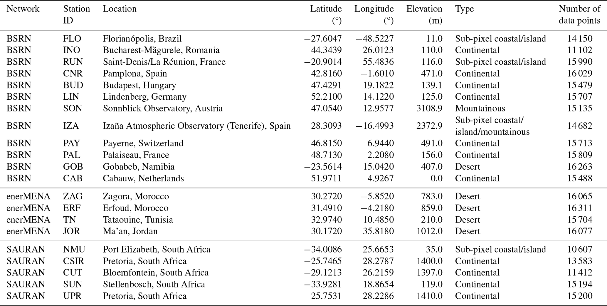
Ground-based sensors contribute localized measurements of atmospheric conditions, enhancing model validation and calibration efforts. Figure 1 and Table 1 shows the locations and information of the ground-based solar radiation stations used in the study. These ground observations were obtained through the THREDDS server catalog (Webservice-Energy, 2025), which is also the basis for the CRS periodical evaluation and quality checks (CAMS Radiation Service, 2025). This catalogue contains 1 min resolution irradiance and meteorological observations from high quality measurement networks worldwide. An interactive online viewer/downloader of the data is available (IN-SITU, 2025). This database is updated every 15 d with the newest available data collected from various measurement networks. For this study, we used year 2021 and stations from 3 high quality measurement networks were selected:
- BSRN:
-
the Baseline Surface Radiation Network (Driemel et al., 2018) is a part of the World Climate Research Program (WCRP). BSRN stations provide ground-based datasets of GHI, BNI, and the diffuse horizontal irradiance (DHI) component in a 1 min temporal resolution. The quality control procedures are described in the Long and Dutton report (Long and Dutton, 2022).
- enerMENA:
-
enerMENA is a project fully named “Towards a Sustainable Implementation of Solar Thermal Power in the MENA Region”. MENA represents the Mediterranean Europe and Northern Africa regions. It includes a dedicated ground measurement program “enerMENA meteo network” applying ventilated CMP21 Secondary Standard Kipp & Zonen pyranometers and Kipp & Zonen CHP1 First Class pyrheliometer instruments at various locations in Northern Africa. This network is described in Schüler et al. (2016).
- SAURAN:
-
the Southern African Universities Radiometric Network (SAURAN) aims to make high-resolution, ground-based solar radiometric data available from stations located across the Southern African region, including South Africa, Namibia, and Botswana. The stations provide high quality radiometric data, using state of the art radiometers, as well as a range of metrological data. Data is available in minute averaged intervals. Information and data can be found on (SAURAN, 2025).
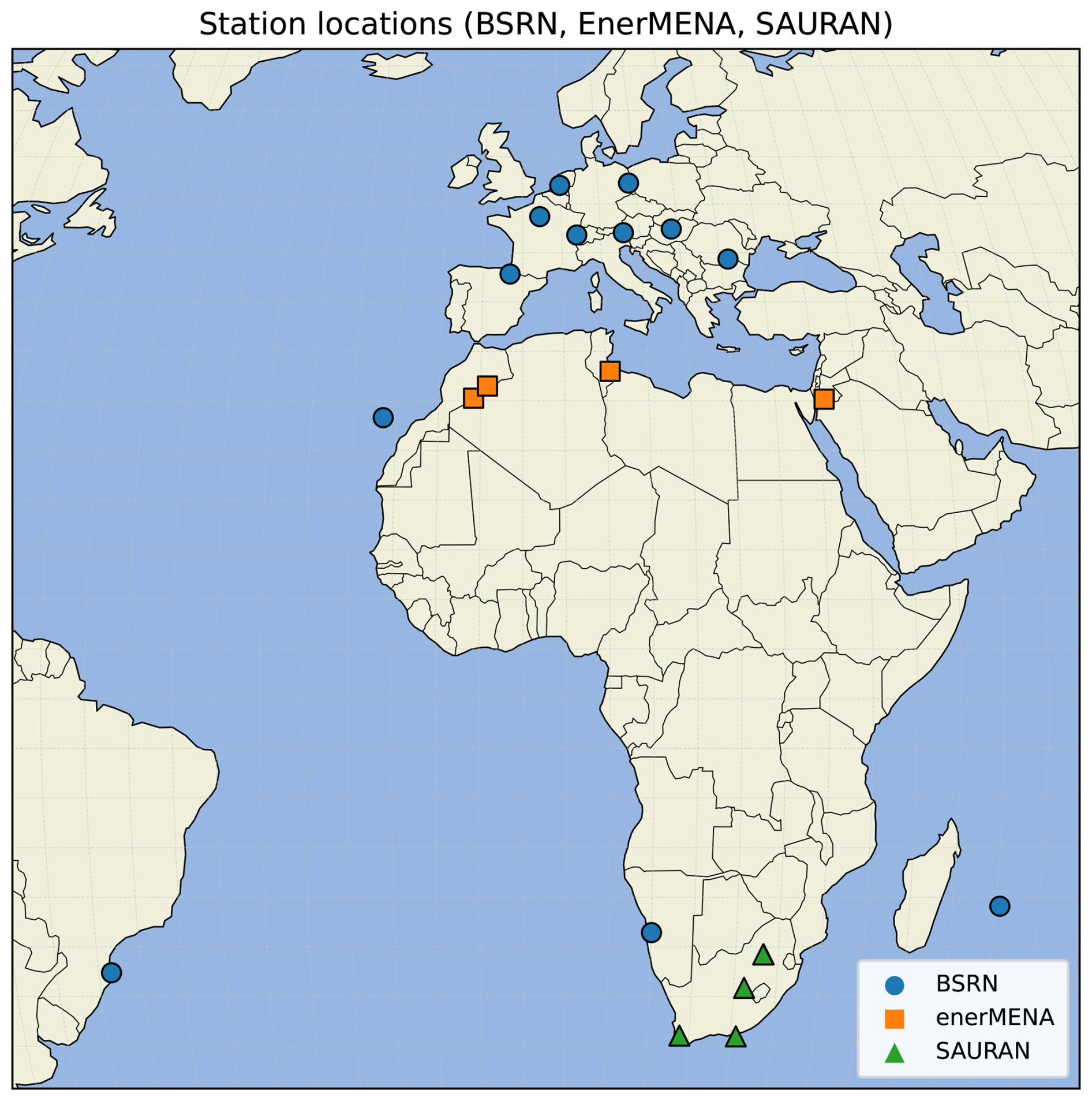
Figure 1Map of ground-based solar radiation stations used in the study.
Table 1Ground-based stations used in this study, including geographic location, elevation and site type, and the number of data points.
To ensure temporal consistency and reduce high-frequency variability at a point observation, the ground-based solar radiation measurements were averaged around the actual pixel observation time from centered 15 min intervals prior to analysis. The 15 min averaging window was selected to reduce the influence of short-term fluctuations in surface irradiance caused by cloud variability and to improve representativeness between point measurements and CRS estimates. While shorter averaging windows would better preserve rapid irradiance changes, they would also be more sensitive to timing mismatches and sub-pixel cloud variability. The selected averaging interval therefore represents a compromise between temporal resolution and collocation robustness.
2.3 Error correction model
In this study, we develop a machine-learning-based residual correction model for the CRS irradiance products. Note that the deviation between CRS and point-wise ground observations is called error in the following. Our model stems from the theoretical premise of an ideal radiative transfer model, which perfectly describes the atmospheric radiative transfer of global radiation at a point observation. Naturally, the ideal radiative transfer model does not exist in practice when input knowledge has other spatial and temporal resolution and lacks detail of optical properties of the atmospheric situation in the individual case. We write the model as
where g represents the global radiation and f is the ideal radiative transfer model with ideal input parameters xideal, including the necessary information to simulate atmospheric radiative transfer such as the state of the atmosphere and solar geometry.
In practice, the radiative transfer model inputs, such as the atmospheric state, are uncertain or partly unknown. Furthermore, often linearly interpolated lookup tables are used to evaluate the model due to limited computational resources and time limitations set by the operational applications resulting, for example, in interpolation errors. We denote the approximate radiative transfer model as = . The approximations and simplifications in lead to inaccurate global radiation predictions; thus, the model does not produce the same outputs as the ideal model f(xideal).
In practice, the CRS radiative transfer model is only an approximation of the ideal atmospheric radiative transfer because its inputs are uncertain or partly unknown and additional approximations as, for example, plane parallel atmosphere assumption, single pixel approximation, average cloud or aerosol optical properties or a linear temporal interpolation of input parameters are introduced by the operational implementation. Consequently, the CRS estimates differ systematically from the corresponding ground-based observations, but differently for each time stamp and location. In this study, this residual, or error, e is used as the target variable for the machine-learning model. Furthermore, it is aimed at quantifying the remaining residual from the operationally available parameters itself – without the need for any auxililary or ground truthing data which is not available in an operational context.
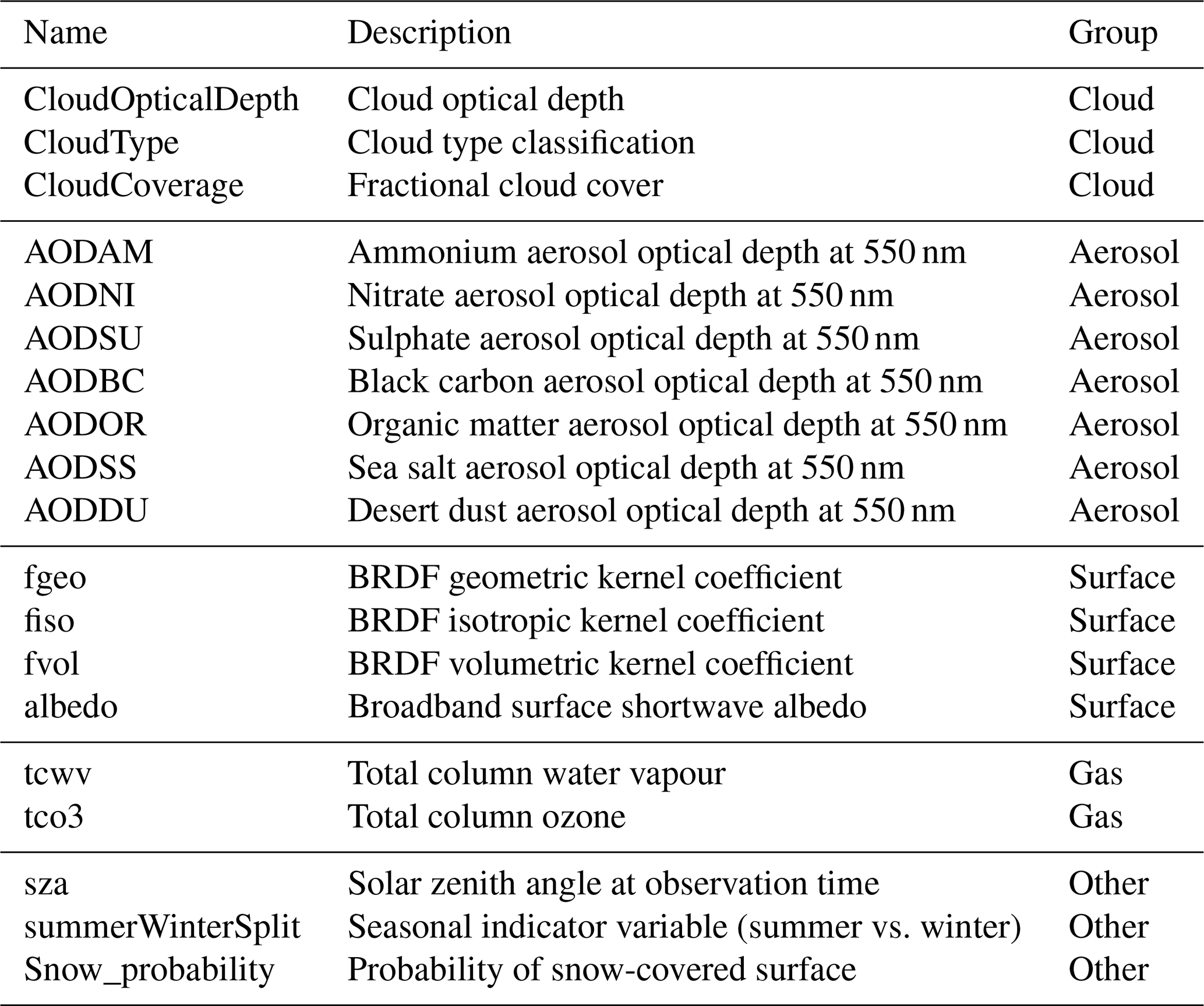
Machine learning approaches typically directly predict g given xideal based on training data. We refer this approach to the fully-learned retrieval approach. In our work, however, we do not take the fully-learned approach but develop a machine-learning-based model to predict the error e instead of g. We train a machine-learning model h(xapproximate)≈e using the operational CRS input parameters listed in Table 3.
Once trained, the error prediction model h is then employed in practical applications to adjust the predictions from , effectively bias-correcting the solar radiation estimates as follows:
This methodology synergistically combines the predictive power of the traditional physics-based radiative transfer model and the data-driven error-correcting capabilities of the machine-learning model h.
Rather than predicting the irradiance directly with the fully learned approach, the machine-learning model is trained to predict the residual between the CRS estimate and the ground-based observation. This residual-learning approach is adopted because the CRS radiative transfer model already captures the dominant physical controls of surface irradiance. The machine-learning model therefore focuses on learning the remaining systematic residual patterns. Compared with the fully learned direct irradiance prediction, this approach preserves the physical modelling framework while providing a practical post-processing correction for the operational CRS products.
The residual-learning approach of predicting the error in an approximate model rather than the fully learned approach has been demonstrated to result in more accurate predictions and requiring less training data compared to fully learned models in many applications (Lipponen et al., 2013, 2018). Moreover, the insights derived from the error correction model h and sensitivities to its inputs can provide valuable information about the weaknesses inherent in the original radiative transfer model . Such insights can be used to enhance the predictive accuracy of the models and they serve as a crucial tool for refining and improving the underlying physical radiative transfer models.
2.4 Extreme gradient boosting
Extreme Gradient Boosting (XGBoost; Chen and Guestrin, 2016) is a widely used tree-based machine-learning algorithm that belongs to the family of gradient boosting methods (Friedman, 2001; Natekin and Knoll, 2013). Its popularity stems from its high predictive accuracy, computational efficiency, and robustness in modelling nonlinear relationships in large and heterogeneous datasets. XGBoost has been successfully applied to a broad range of regression and classification tasks, including several atmospheric and environmental applications where complex, interacting processes must be represented in a data-driven manner (e.g. Ma et al., 2020; Dong et al., 2023; Zhen et al., 2024).
XGBoost builds an ensemble of regression trees in a sequential boosting framework. Each new tree is trained to correct the residual errors of the ensemble formed by the preceding trees, thereby iteratively improving the model. The optimisation is performed using gradient descent on the chosen loss function, typically the mean squared error in regression problems. The model includes several regularisation mechanisms, such as penalisation of tree complexity, shrinkage (learning rate), and column subsampling, that help prevent overfitting and enhance generalisation. Tree growth is controlled through both depth limitation and XGBoost pruning while growing strategy, which halts node splitting when the expected gain falls below a threshold, improving computational efficiency.
In this study, XGBoost is used to model the instantaneous CRS irradiance residual for each irradiance component (GHI, DHI, BNI). For both parts of the study, three separate regression models are trained using the same 19 operational predictors listed in Table 3 and the mean squared error loss function. The diagnostic and predictive parts nevertheless use different fitted models because their aims and evaluation requirements differ.
The diagnostic models are used only for the SHAP analysis. For each irradiance component, 100 000 rows were sampled from the overall analysis dataset using a fixed sampling seed. Ten models were fitted to these sampled rows using random seeds 1–10, max_depth = 15, colsample_bytree = 0.3, learning_rate = 0.9, and 100 boosting rounds. The resulting SHAP values were pooled across the ten fits to characterise the behaviour learned by these models over the sampled training distribution. Consequently, the main diagnostic SHAP results are explicitly in-sample and they describe how the fitted diagnostic models represent the analysed residuals and do not estimate predictive performance on unseen observations. This choice is consistent with the diagnostic aim of describing the residual structure represented in the available collocated dataset, evaluating SHAP only on held-out observations would instead address the different question of whether the learned relationships generalise beyond the fitted data. The large pooled sample supports a detailed description of the fitted diagnostic models over these cases, but it does not establish that every learned pattern is stable outside these data. Because SHAP decomposes both general structure and any sample-specific structure learned by a flexible model, we emphasise broad feature-group patterns and treat detailed individual-feature rankings as model-dependent. Moreover, it is important to note that using the training distribution does not remove measurement, retrieval, collocation, or point-pixel representativeness contributions already present in the target residual, it only avoids adding an out-of-sample generalisation question to the diagnostic analysis. The corresponding training and validation learning curves are shown in Fig. C1. The gap between training and validation RMSE further illustrates the high flexibility of the diagnostic models and motivates the cautious interpretation of detailed feature rankings.
The predictive correction models are designed and evaluated separately. To avoid leakage between temporally adjacent 15 min averages, complete station-day groups were assigned to training, validation, and test partitions in proportions of 70 %, 15 %, and 15 %, respectively, using the deterministic seed 20260901. Dates were assigned separately within each station so that all 21 stations were represented in every partition, and no station-day group occurred in more than one partition. The resulting training, validation, and test sample counts were 199 292, 42 147, and 43 613 for GHI; 199 300, 42 148, and 43 614 for DHI; and 175 376, 37 386, and 39 023 for BNI.
Although grouping complete station days prevents individual 15 min averages from the same day from appearing in different partitions, consecutive days can still be assigned to different partitions. Consequently, persistent synoptic situations and slowly varying predictors, such as aerosol optical depth, total column water vapour, and surface properties, may remain correlated across partition boundaries. The station-day evaluation should therefore be interpreted as generalisation to unseen days at represented stations rather than as a test of independence across longer synoptic periods.
For each component, we evaluated 1350 hyperparameter combinations. The search covered learning rates η of 0.025, 0.05, 0.10, 0.20, and 0.40; maximum depths of 4, 6, 8, 10, and 15; minimum child weights of 1, 5, and 15; row subsampling fractions of 0.70 and 0.90; and column subsampling fractions of 0.60, 0.85, and 1.00. Three regularisation profiles were tested: , , and . Validation RMSE was used for model selection. Training was limited to 3000 boosting rounds, with early stopping after 100 rounds without improvement in validation RMSE. After selecting the hyperparameters (Table 2) and number of boosting rounds, each final correction model was refitted on the combined training and validation partitions and evaluated once on the untouched test partition. No test result was used for model selection.
Spatial generalisation was assessed in a leave-one-station-out (LOSO) sensitivity analysis. For each of 21 folds and each irradiance component, all usable observations from one station were withheld, the model was fitted using the other 20 stations, and predictions were generated for all usable observations at the omitted station. The hyperparameters and number of boosting rounds were frozen at the values selected in the previous station-day search, and no LOSO outcome was used for further tuning. Results were calculated both for each omitted station and after pooling the predictions from all folds.
To assess whether the station-day correction skill could mainly reflect persistent station-specific biases, we additionally constructed a simple station-mean residual baseline. For each irradiance component and station, the mean CRS residual was calculated using only the training partition and applied as a constant correction to observations from the same station in the untouched test partition. We also repeated the predictive correction experiments after removing the four surface predictors fgeo, fiso, fvol, and albedo. The same data partitions, LOSO folds, hyperparameters, and numbers of boosting rounds as for the corresponding full-feature correction models were used in this sensitivity test.
Table 2Selected hyperparameters for the predictive correction models. The number of boosting rounds was selected by early stopping on the validation partition before refitting on the combined training and validation data.

XGBoost was selected for this study because of its strong predictive performance, robustness, and compatibility with the exact TreeSHAP algorithm used for feature attribution. The objective of this study is not to identify the optimal machine-learning algorithm, but to investigate residual error attribution within an explainable machine-learning framework. Consequently, a comprehensive comparison against alternative regression methods was considered outside the scope of the present work.
Table 3Input features of the error model. Data source for all inputs is CRS.
2.5 SHapley Additive exPlanations (SHAP) analysis
SHAP analysis provides a theoretically grounded framework for interpreting machine learning models by quantifying the contribution of each input feature to individual predictions. The method is rooted in cooperative game theory, where Shapley values (Shapley, 1953) distribute the total payoff of a game among players according to their marginal contributions. In a machine-learning context, the ”players” correspond to input features and the SHAP value of a feature represents its contribution to a specific model prediction relative to a baseline.
SHAP analysis (Lundberg and Lee, 2017) aims to provide a unified measure of feature importance that is both consistent and locally accurate. Consistency ensures that if a model changes so that a feature's contribution increases or remains unchanged, its attributed importance should not decrease. Local accuracy refers to the ability of SHAP values to perfectly decompose a model's prediction into the sum of the effects of each feature for a given instance. This property is crucial for detailed insight into complex models. These properties are especially valuable for interpreting nonlinear models with complex feature interactions, such as gradient boosted trees.
Exact computation of SHAP values requires evaluating all possible feature subsets, which is computationally infeasible for realistic problems. In this work, we use TreeSHAP, an algorithm specifically developed for tree-based models that exploits their structure to compute SHAP values efficiently (Lundberg et al., 2020). TreeSHAP enables the use of SHAP analysis for large datasets and high-dimensional feature sets, such as those used in the CRS radiation processing chain. For all SHAP computations, we use the Python SHAP package (Lundberg and Lee, 2017).
In this study, SHAP serves two complementary purposes. First, it provides a dataset-level diagnostic of the physical features associated with CRS irradiance errors. We use SHAP beeswarm plots to analyse the distribution of feature contributions across all samples and we group the features into physically meaningful categories (cloud, aerosol, gas, surface, and other) to assess their aggregate behaviour. Second, SHAP is used to investigate how error contributions change with solar geometry by computing group-wise mean absolute SHAP values in solar-zenith-angle bins, using SZA as a representative example of how the framework can resolve dependencies on individual physical features associated with CRS irradiance errors. This enables us to identify SZA-dependent error mechanisms. Finally, we apply SHAP to individual samples, allowing us to interpret the error sources in specific a situation, such as the overcast case detailed in Sect. 3.4. Together, these SHAP analyses provide a model-based diagnostic of the CRS residual characteristics. The main SHAP results explain the diagnostic models rather than the separately tuned predictive correction models described in Sect. 2.4. As a sensitivity test, however, we additionally calculated group-wise SHAP importance for the correction models on their held-out test sets and compared the resulting feature-group hierarchy with that obtained from the diagnostic models.
Although SHAP provides a theoretically well-founded framework for feature attribution based on Shapley values from cooperative game theory, strongly correlated predictors may share explanatory power, resulting in some ambiguity in the attribution assigned to individual variables. Consequently, the exact ranking of individual predictors should be interpreted with caution. In this study, we therefore also consider broader feature groups when interpreting the results, in addition to individual features.
We analysed the SHAP values of the diagnostic XGBoost residual models separately for global horizontal irradiance (GHI), diffuse horizontal irradiance (DHI) and beam normal irradiance (BNI). As described in Sect. 2.4, these are explanations of diagnostic models and must not be interpreted as out-of-sample correction results. On the held-out test partitions used later for correction evaluation, the original CRS products achieve coefficients of determination of 0.866, 0.584, and 0.655 for GHI, DHI, and BNI, respectively (Sect. 3.5). In all cases, the target variable is the residual between the CRS estimate and the corresponding ground-based observation: EGHI = GHIobs − GHICRS. Positive SHAP values therefore indicate conditions in which the CRS radiation model tends to underestimate the corresponding irradiance component, that is the observed irradiance is larger than the CRS irradiance, whereas negative SHAP values indicate CRS model irradiance overestimation.
As a sensitivity test, we calculated group-wise SHAP importances for the predictive correction models using their held-out test sets. Although these test sets contain substantially fewer samples than the diagnostic SHAP analysis, the broad feature-group attribution was consistent between the two model families. Cloud-related predictors remained the most important group for GHI, DHI, and BNI, while the detailed contributions of the secondary aerosol, surface, and gas groups showed some model dependence. This comparison supports the robustness of the main conclusion of cloud-dominated residual structure, while the detailed individual-feature interpretations below are based on the diagnostic models.
It should be noted that the residuals analysed here contain not only the deficiencies in the CRS radiative transfer modelling, but also measurement uncertainty, representativeness differences between point observations and satellite-scale pixels, and collocation and retrieval errors. Consequently, the SHAP analysis identifies the factors associated with the total residual rather than isolating individual physical error sources. Also, under broken-cloud conditions the point-pixel representativeness mismatch may covary with cloud optical depth, cloud coverage, and cloud type. Part of the high SHAP importance assigned to cloud optical depth may therefore represent scene-dependent mismatch that cannot be removed through straightforward improvements to the radiative transfer calculations alone. The high quality of the ground-based observations limits, but does not eliminate, the observational uncertainty of the analysis. The feature attributions must therefore be interpreted as associations learned by the diagnostic models rather than as unique or causal decompositions of CRS model error. This is very much in line with practical applications in the solar energy sector, where users of the CRS face a similar challenge to understand the need between CRS data and their local ground observations or power production data. Therefore, this approach is also helpful from the CRS user's perspective.
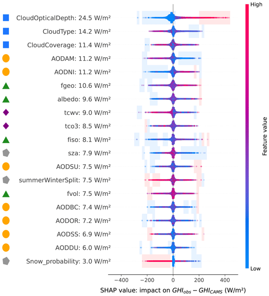
For each component, we show the SHAP beeswarm plots that summarise the feature-level behaviour over the whole data set. In the beeswarm plots, individual features are ordered by their importance (mean absolute SHAP value) so that the most important feature is shown at the top and colors indicate the corresponding feature values. Symbols on the left edge of the beeswarm plots indicate the feature group (cloud, aerosol, surface reflectance, gas, others) each feature variable belongs to. We also show the SZA binned plots to quantify how the mean absolute contribution of feature groups varies with solar geometry. In the SZA-binned plots, the SHAP values are first summed over all features belonging to a given group, and the mean absolute value of this group-level contribution is then computed in SZA bins and normalised by the total irradiance. Together, these figures allow us to identify the key features associated with CRS errors for each irradiance component and to assess how these error patterns change systematically with SZA.
3.1 Global horizontal irradiance (GHI)
For GHI, the beeswarm plot in Fig. 2 shows that cloud-related variables dominate the error budget. Cloud optical depth has the largest mean absolute SHAP value (24.5 W m−2), followed by cloud type and cloud coverage. Among all features, cloud optical depth is the only variable exhibiting a well-defined SHAP–feature relationship: high optical depths consistently correspond to positive SHAP values, indicating GHI underestimation by CRS under optically thick clouds, while low optical depths tend to produce negative SHAP values, consistent with GHI overestimation in thin-cloud or near-clear conditions. Cloud type and cloud coverage, despite their high importance, show no monotonic or structured dependence on SHAP values, with both low and high feature values appearing across the entire SHAP range.
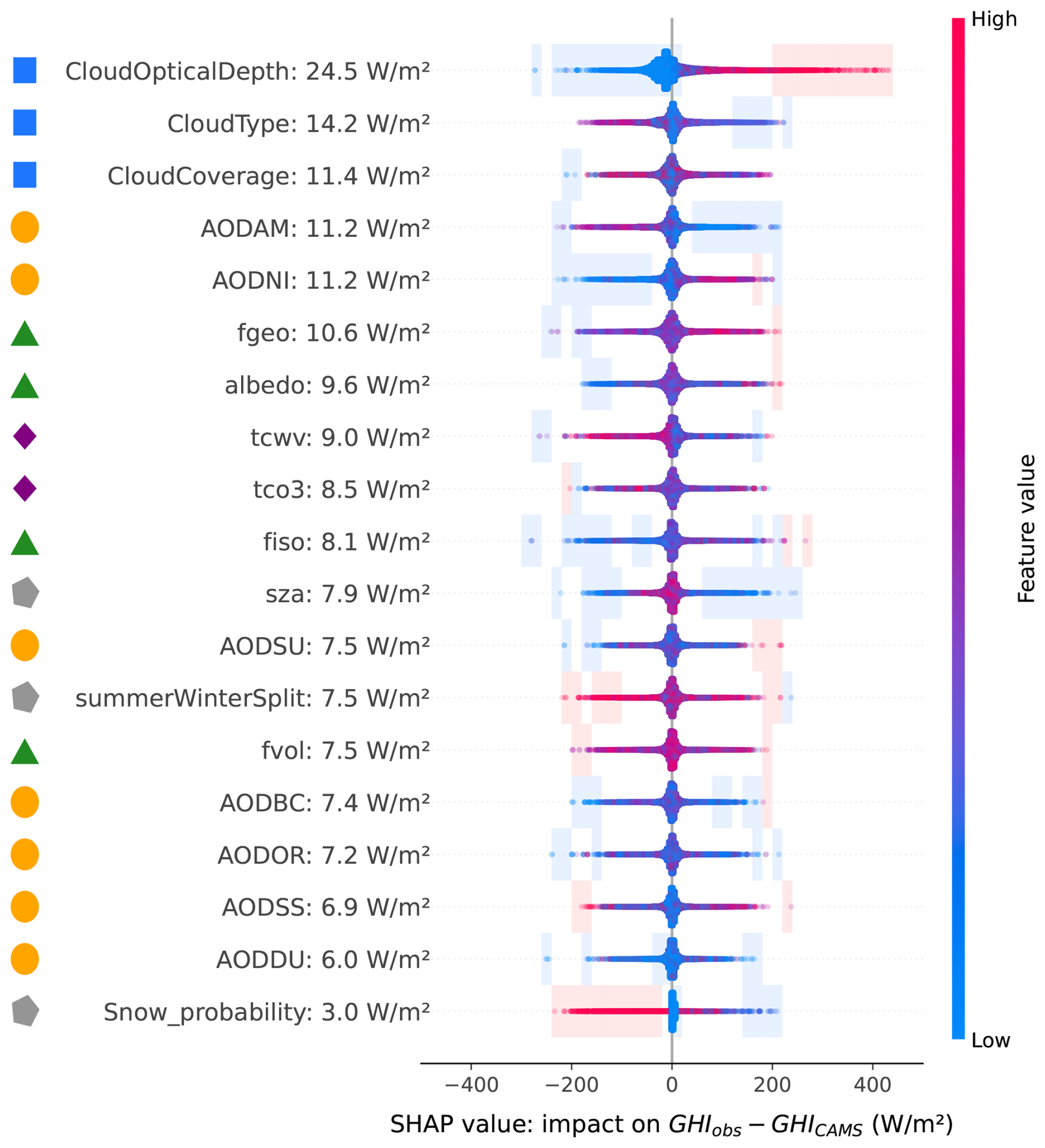
Figure 2SHAP beeswarm plot for the diagnostic GHI residual model defined as GHIobs − GHICRS. Input variables are ordered by their mean absolute SHAP value, indicating their overall importance within the fitted diagnostic models. Each point represents an individual sample model-observation attribution, with the horizontal position showing the SHAP value (impact on the predicted error) and the color indicating the corresponding feature value (blue: smaller than average, red: larger than average). For visualisation purposes, points are vertically displaced within each feature row in regions of high sample density. Shaded regions highlight areas where more than 90 % of the SHAP contributions originate from either larger-than-average (red shading) or smaller-than-average (blue shading). Symbols on the left denote feature groups (cloud, aerosol, surface, gas, and other variables). Positive SHAP values indicate conditions contributing to CRS GHI underestimation, while negative values indicate CRS GHI overestimation.
Aerosol, surface, and gas variables form the next group of influential predictors. Aerosol species AODAM and AODNI show substantial contributions but no consistent SHAP–feature pattern. This finding is interesting because these two inorganic aerosol species, ammonium and nitrate, were recently added to CRS (Peuch et al., 2022). Their elevated importance suggests that ammonium- and nitrate-related aerosol information is associated with the analysed residuals. However, SHAP values alone do not identify the underlying physical causes of the residuals. Possible explanations include uncertainties in the aerosol retrievals, representativeness errors, correlations with other predictors, or deficiencies in the aerosol representation within the CRS modelling framework for example in cases of polluted environments. Furthermore, AODAM and AODNI are strongly correlated in the input dataset (correlation coefficient 0.95) indicating that their nearly identical mean absolute SHAP values should not be interpreted as independent species-specific contributions. Surface parameters fgeo and albedo also lack a clear SHAP structure with high and low feature values present on both sides of the SHAP distribution. This indicates a non-monotonic but important sensitivity of GHI to surface reflectance. Gas variables tcwv and tco3 similarly affect the error but without an interpretable pattern. Snow_probability is the only lower-ranked variable with a clear tendency: snow-free scenes correspond mostly to near-zero SHAP values, while snow-covered scenes can produce either positive or negative SHAP contributions.
The SZA-binned group-wise contributions in Fig. 3 confirm the significance of clouds across most of the SZA range with sharply increasing importance at SZAs exceeding 70°. Aerosols dominate at the lowest SZAs and remain the second most influential group elsewhere, while surface variables form the third most important group with a gradual rise toward large SZAs. Gas and other variables contribute the least, though their contributions remain non-zero. It should be noted that the lowest SZA bins contain observations from only a limited number of stations as many locations in the dataset never experience such small solar zenith angles. Consequently, the patterns at very low SZAs represent a smaller and geographically restricted subset of the full dataset.
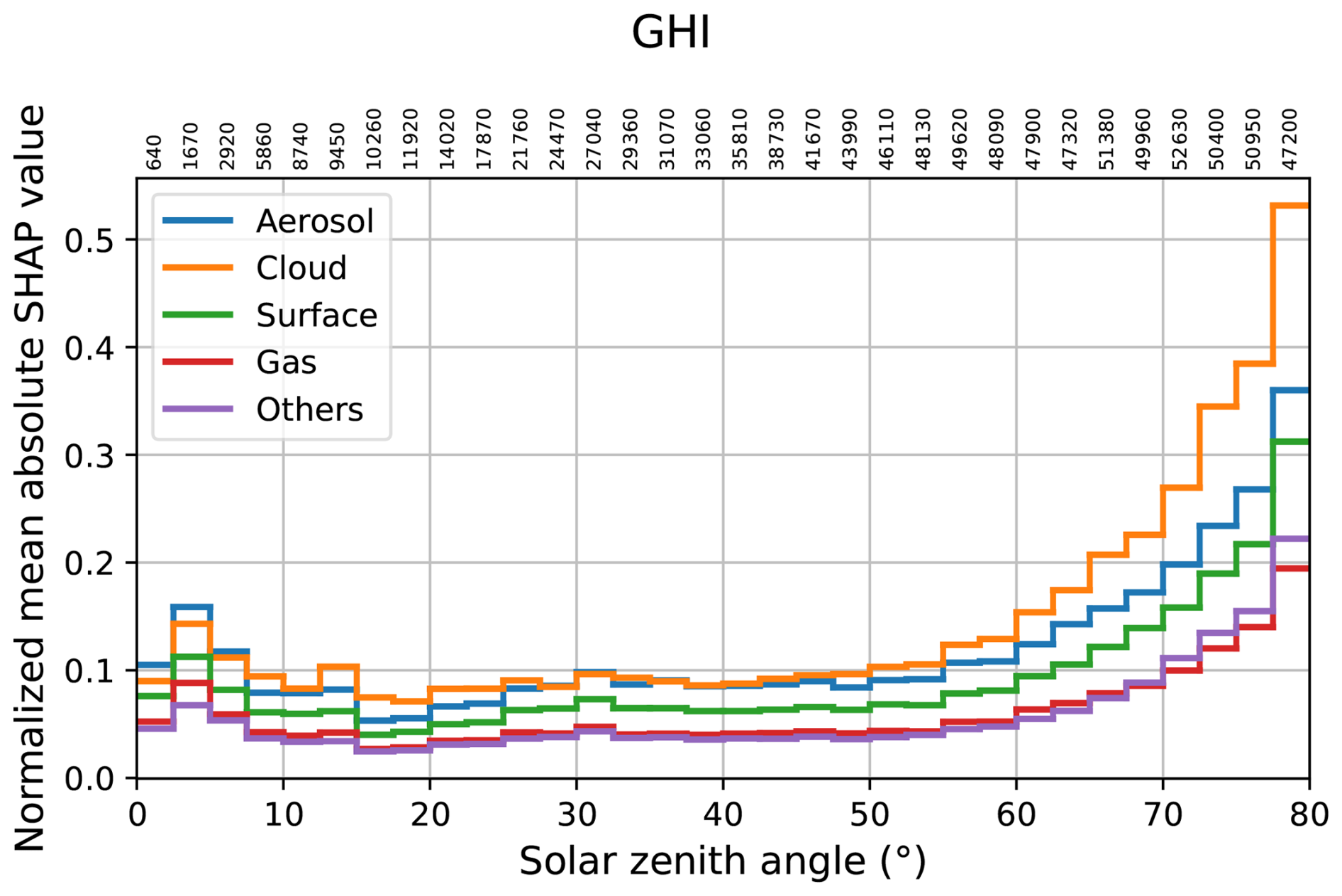
Figure 3Mean absolute group-wise SHAP contributions from the diagnostic models, normalised by total GHI, as a function of solar zenith angle. Each curve represents the sum of SHAP values over a feature group. Solar zenith angle is binned using 2.5° intervals over the range 0–80°. The numbers shown above the x axis indicate the number of samples within each solar zenith angle bin.
From a modelling perspective, cloud optical depth retrievals and the physical consistency among cloud properties are priority areas for further investigation, especially at large SZAs. Aerosol and surface-related associations are also present, but their non-monotonic behaviour and correlations with other predictors prevent the SHAP analysis from identifying a unique process or parameterisation responsible for these residuals. Overall, the GHI SHAP analysis identifies cloud, aerosol, and surface predictors associated with the fitted residuals and shows that the strength of these associations varies with SZA.
3.2 Diffuse horizontal irradiance (DHI)
For DHI, cloud optical depth is again the most influential feature, although the SHAP magnitudes are smaller than for GHI, see Fig. A1 in Appendix A. This reflects the smaller dynamic range of DHI and the more indirect coupling between radiative transfer errors and the diffuse component. As in the GHI case, cloud optical depth is the only cloud variable with a clear SHAP–feature relationship: high optical depths lead to positive SHAP values, indicating DHI underestimation under strong scattering, while low optical depths tend to produce negative SHAP values, consistent with overestimation in thin-cloud or cloud-free conditions. Cloud coverage and cloud type, by contrast, do not show monotonic or structured SHAP patterns, even though both remain among the higher-importance predictors.
Surface variables also contribute substantially to the DHI error. The BRDF geometric kernel coefficient fgeo ranks directly after cloud optical depth but shows no monotonic SHAP–feature structure. Both high and low surface reflectance conditions can lead to positive or negative SHAP values. The two most influential aerosol predictors, AODNI and AODAM, similarly show no consistent SHAP pattern. Gas variables tcwv and tco3 contribute modestly but without a monotonic dependence. Most other variables display no recognisable SHAP–feature structure. Snow_probability is a notable exception and snow-free scenes correspond almost exclusively to zero SHAP values, while snow-covered scenes yield non-zero SHAP values of either sign indicating that snow can shift the DHI error toward higher or lower values depending on the conditions.
The SZA-binned group-wise contributions in Fig. A2 in Appendix A provide additional insight. Aerosols dominate the normalised SHAP contributions across nearly all SZAs, particularly at small SZAs. However, the lowest SZA bins contain substantially fewer observations and originate from a more limited subset of stations than the higher SZA bins. Consequently, this result should be interpreted with caution. Clouds form the second most important group and increase steeply at SZAs greater than 70° reflecting the enhanced role of cloud representation as the direct beam weakens and diffuse multiple scattering becomes dominant. Surface variables consistently form overall the third most important group, and even the second most important group at SZAs 10–60°, and increase slightly with SZA. Gases and other variables contribute least.
The importance of aerosol-related predictors suggests that aerosol information is associated with the analysed DHI residuals, but the rankings of individual aerosol species are exploratory. However, SHAP values alone do not identify the underlying physical causes of the residuals. Possible explanations include aerosol retrieval errors, scattering geometry effects, representativeness errors, correlations with other predictors, or deficiencies in the aerosol representation within the CRS modelling framework. The surface-related associations similarly motivate further investigation of bright or anisotropic surface conditions. Overall, the DHI SHAP analysis indicates that cloud, aerosol, and surface information is jointly associated with the fitted DHI residual and that these associations are SZA-dependent.
3.3 Beam normal irradiance (BNI)
BNI exhibits the strongest absolute SHAP magnitudes among the three irradiance components, reflecting the high sensitivity of the direct beam to atmospheric extinction. Cloud optical depth is the most influential predictor, see Fig. A3 in Appendix A. Low cloud optical depths tend to produce negative SHAP values, indicating that CRS overestimate BNI in cloud-free or thin-cloud situations. However, the positive SHAP values do not follow a clear monotonic feature–SHAP relationship and both small and large cloud optical depths can correspond to positive SHAP values. Cloud coverage and cloud type also rank highly, yet – similar to their behaviour in GHI and DHI and neither of them exhibits a well-defined SHAP–feature structure.
It is noteworthy that the BRDF geometric parameter fgeo appears as the third most important predictor for BNI even though the direct beam should be only weakly affected by surface reflectance under ideal radiative transfer conditions. Therefore, the relatively high importance of the BRDF-related parameters is somewhat unexpected given the weak direct influence of surface reflectance on the direct beam component. However, SHAP values identify variables associated with the analysed residuals rather than direct physical causes. This behaviour likely reflects indirect effects rather than a direct physical influence of the surface on the beam. Specifically, fgeo may act as a proxy for scene characteristics that co-vary with BNI error, such as surface type, unresolved sub-grid cloud geometry, or cloud–surface contrast affecting the cloud retrievals used by CRS. The correction model sensitivity experiment provides an additional possible interpretation: because the surface parameters vary relatively slowly at individual stations, they may also contain location specific information. Removal of surface features has only a small effect on the station-day correction, but it improves LOSO generalisation suggesting that part of their predictive importance may be associated with station environment rather than a direct physical influence on BNI. SHAP identifies fgeo as an important predictor because it improves error estimation, even though the feature does not directly affect the beam irradiance. This highlights the usefulness of SHAP in identifying variables associated with the analysed residuals, including indirect predictors that capture systematic patterns in the CRS processing chain.
Total column water vapour (tcwv) is more influential for BNI than for GHI or DHI, ranking fifth in importance for BNI error overall. Its SHAP pattern shows that most of the large positive SHAP values correspond to small tcwv values, whereas negative SHAP values occur across a broader tcwv range without a clear dependency pattern. Aerosol predictors, particularly AODNI and AODAM, also rank among the most important features, but similarly as for the other irradiance components they do not show a consistent SHAP–feature relationship. Large SHAP values can occur at both low and moderate aerosol optical depths. Because the species-specific aerosol optical depths are correlated, their individual rankings are not unique and are treated as exploratory and the result does not necessarily demonstrate inaccurate optical properties of ammonium or nitrate.
The SZA-binned group-wise contributions in Fig. A4 in Appendix A highlight the dominant role of clouds across the entire SZA range, with a pronounced rise in relative importance above 70° where the direct beam is strongly attenuated. Aerosols and surface variables form the second and third most influential groups, with broadly similar magnitudes and no clear separation between them. Gas and other variables contribute least but remain consistently non-zero. All variable groups exhibit an increase in SHAP contributions at SZAs exceeding approximately 50°, indicating that uncertainties in cloud, aerosol and surface representations are amplified as the solar path length increases and extinction effects become more pronounced.
From a modelling perspective, the results motivate further investigation of cloud optical depth retrievals, particularly for thin and broken clouds where detection, classification, and point-pixel representativeness are challenging. The aerosol and surface associations identify additional conditions and inputs to examine, but their non-monotonic SHAP patterns and predictor correlations do not support attributing the residuals to a specific aerosol optical property or surface parameterisation.
3.4 Case examples: single-sample SHAP analysis
To illustrate how SHAP analysis can be used to interpret individual irradiance residuals, we analyse two cases. The first case represents overcast cloudy conditions, while the second represents a cloud-free situation with elevated aerosol loading. These examples are not intended to be statistically representative of the full dataset, but to demonstrate how the trained error model decomposes individual residual predictions into contributions from different CRS input variables.
The first case is from the WRMC–BSRN station in Palaiseau, France, on 14 November 2021 at 09:26 UTC. The scene was overcast, with CRS cloud coverage of 100 %, cloud optical depth of 77.6, and solar zenith angle of 72.9°. The CRS strongly underestimated all three irradiance components: the observed and CRS values were 133 and 28 W m−2 for GHI, 112 and 24 W m−2 for DHI, and 51 and 13 W m−2 for BNI, respectively. In the corresponding SHAP waterfall plots, Fig. 4, left column, the cloud optical depth is the dominant positive contributor for all three components. This indicates that the very large cloud optical depth is strongly associated with the positive residuals meaning CRS underestimation in this case. The result is consistent with the interpretation that the modelled cloud extinction is too strong for this scene, although the residual may also include representativeness and retrieval effects.
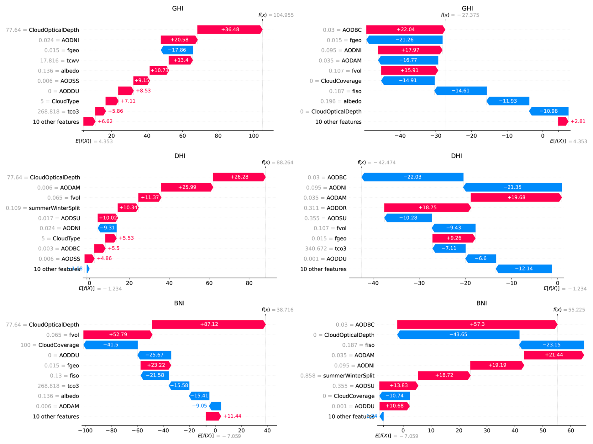
Figure 4SHAP waterfall plots illustrating the decomposition of the predicted CRS irradiance residuals for two individual cases. The left column shows the WRMC–BSRN Palaiseau station on 14 November 2021 at 09:26 UTC under overcast conditions (cloud coverage 100 %, cloud optical depth 77.6, solar zenith angle 72.9°). The right column shows the WRMC–BSRN Cabauw station on 5 August 2021 at 17:11 UTC under cloud-free but aerosol-loaded conditions (cloud coverage 0 %, cloud optical depth 0, total aerosol optical depth approximately 0.83, solar zenith angle 71.6°). Rows show results for global horizontal irradiance (GHI, top), diffuse horizontal irradiance (DHI, middle), and beam normal irradiance (BNI, bottom). Each plot starts from the error-model mean prediction E[f(X)] and shows how individual input features contribute to the final predicted residual f(x). Positive SHAP values increase the predicted residual, corresponding to conditions associated with CRS underestimation, while negative SHAP values decrease the predicted residual, corresponding to conditions associated with CRS overestimation. The grey values indicate the corresponding CRS input values.
Surface and aerosol variables also contribute to the decomposition of the overcast case, but their interpretation is less direct. For BNI, the BRDF volumetric parameter fvol is the second-largest positive contributor, suggesting that surface-related variables can act as indirect predictors of residual patterns even for the direct-beam component. Aerosol-related variables also appear in the SHAP decomposition, although the CRS aerosol optical depths are very small in this case (e.g. AODAM = 0.006, AODNI = 0.024, AODSS = 0.006). At such low aerosol loadings, their direct radiative influence is expected to be limited and uncertainties in the aerosol inputs may be comparable to the reported values. Therefore, these aerosol-related SHAP contributions should not be interpreted as direct evidence of aerosol extinction errors. They may instead reflect interactions with other predictors, retrieval uncertainties, representativeness effects, or broader environmental conditions associated with the residual.
The second case is from the WRMC–BSRN station in Cabauw, the Netherlands, on 5 August 2021 at 17:11 UTC. In contrast to the Palaiseau example, this was a cloud-free scene in the CRS data, with cloud coverage and cloud optical depth both equal to zero. The total aerosol optical depth from the CRS aerosol components was high, approximately 0.83, dominated by sulphate and organic matter aerosol optical depths, with additional contributions from nitrate, ammonium and black carbon. The CRS overestimated GHI and DHI, with observed and CRS values of 162 and 190 W m−2 for GHI and 86 and 129 W m−2 for DHI, respectively. For BNI, the CRS underestimated the observation, with observed and CRS values of 247 and 192 W m−2.
The SHAP decompositions for this aerosol-loaded case (Fig. 4, right column) differ clearly from the overcast case. Aerosol-related predictors dominate several of the individual residual estimates. For GHI, AODBC and AODNI provide positive contributions, while AODAM contributes negatively. For DHI, several aerosol components are among the largest contributors, including AODBC, AODNI, AODAM, AODOR and AODSU. For BNI, AODBC is the largest positive contributor, followed by other aerosol-related variables such as AODAM, AODNI, AODSU and AODDU. The signs of the aerosol contributions differ between components and species, possibly indicating that the model uses aerosol information in a component-dependent way rather than as a simple monotonic correction.
Together, the two examples demonstrate how single-sample SHAP analysis can provide a transparent decomposition of the trained residual model under different atmospheric regimes. The overcast case illustrates a residual pattern dominated by cloud optical depth, whereas the cloud-free aerosol-loaded case shows much stronger aerosol-related contributions. These examples also highlight the need for cautious interpretation: SHAP values identify the predictors associated with the modelled residuals, but they do not by themselves prove the underlying physical cause of the CRS error.
3.5 Post-process correction of solar irradiance data
To evaluate predictive post-processing performance without information leakage from training data to test data, all metrics in this section were computed on the untouched test partitions described in Sect. 2.4. The results therefore concern the separately tuned predictive correction models and not the diagnostic models used for the main SHAP analysis. Figure 5 compares the original CRS values with the corrected estimates, and Table 4 summarises the test metrics.

Figure 5Density plots comparing the original CRS and corrected surface solar radiation components against ground-based observations in the untouched station-day test partitions. The left column shows the original CRS estimates, while the right column shows the corresponding estimates obtained with the predictive correction models. From top to bottom, the panels correspond to GHI, DHI, and BNI. The solid black line denotes the 1:1 line. Each panel reports the median and mean bias, mean absolute error, RMSE, and coefficient of determination and their corresponding 5000-sample bootstrapping 95 % percentile intervals.
Table 4Performance of the original and corrected CRS irradiances. Bias denotes the median prediction error, and R2 is the coefficient of determination.

For GHI, RMSE decreases from 106.2 to 87.5 W m−2 (17.6 %) and MAE decreases by 16.5 %, while R2 increases from 0.866 to 0.909. The median bias changes from 4.8 to −4.2 W m−2, indicating that the corrected distribution has a small negative median error. For DHI, RMSE decreases from 76.9 to 61.1 W m−2 (20.5 %), MAE decreases by 22.1 %, and R2 increases from 0.584 to 0.737. The median bias is reduced from 11.4 to 5.3 W m−2. For BNI, RMSE decreases from 204.9 to 155.9 W m−2 (23.9 %), MAE decreases by 16.4 %, and R2 increases from 0.655 to 0.800. However, the BNI median bias changes from −1.9 to −12.0 W m−2 and the mean bias from 1.5 to −5.8 W m−2. Thus, the BNI model substantially reduces the magnitude of large errors while introducing a modest negative overall bias that warrants further calibration.
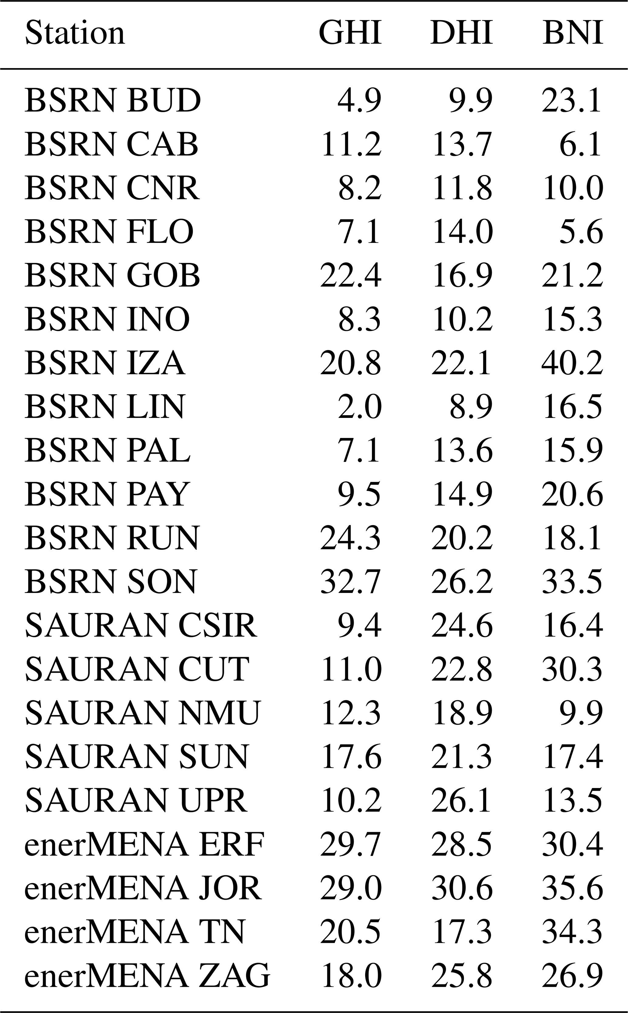
The aggregate results are not driven by a small number of stations. RMSE decreases at every one of the 21 stations for each irradiance component (Table 5). The station-level reductions range from 2.0 %–32.7 % for GHI, 8.9 %–30.6 % for DHI, and 5.6 %–40.2 % for BNI. To estimate the uncertainty of the aggregate RMSE reduction, we resampled complete station-day groups with replacement using 5,000 bootstrap samples. The resulting 95 % percentile intervals for the aggregate RMSE reduction are 16.7 %–18.5 % for GHI, 19.7 %–21.4 % for DHI, and 23.1 %–24.7 % for BNI.
Table 5Station-level reduction in RMSE (%) after applying the predictive correction models. Positive values indicate improvement.
The BNI correction introduces a small negative systematic bias despite substantially reducing RMSE. This is possible because the XGBoost model is optimised for mean squared error and does not explicitly constrain the corrected mean or median bias to zero. Therefore, reduction of large prediction errors can be accompanied by a shift in the centre of the residual distribution.
As an additional sensitivity test, we first compared the XGBoost correction with a simple station-specific mean-residual correction calculated from the training data. This baseline reduced RMSE by only 0.8 %, 2.5 %, and 1.0 % for GHI, DHI, and BNI, respectively, compared with 17.6 %, 20.5 %, and 23.9 % for the XGBoost models. Thus, a constant station-specific residual explains only a small fraction of the XGBoost correction. Removing the four surface predictors fgeo, fiso, fvol, and albedo from the XGBoost models resulted in station-day RMSE reductions of 15.4 %, 18.6 %, and 22.2 % for GHI, DHI, and BNI, respectively. Most of the station-day correction skill is therefore retained without the surface predictors.
3.6 Sensitivity to station location
The station-day evaluation above tests prediction for unseen days while retaining every station in the training data. The LOSO experiment provides an assessment of correction sensitivity to a station location absent from model fitting. After pooling predictions for all omitted stations, GHI RMSE decreases from 105.2 to 103.4 W m−2 (1.7 %), DHI RMSE decreases from 76.3 to 69.9 W m−2 (8.4 %), and BNI RMSE decreases from 202.3 to 201.3 W m−2 (0.5 %). The corresponding changes in MAE are less uniformly favourable: DHI MAE decreases by 7.6 %, whereas GHI and BNI MAE increase by 6.6 % and 13.3 %, respectively. Mean bias changes from 0.8 to −11.7 W m−2 for GHI, from 2.8 to 7.3 W m−2 for DHI, and from 4.4 to −34.0 W m−2 for BNI. The stronger negative BNI bias in the LOSO experiment is consistent with the reduced transferability of the learned correction to station environments absent from training and further indicates that component-specific bias calibration would be required before operational application. The full station-level RMSE changes are given in Table B1 in Appendix B. RMSE improves at 18 of 21 stations for GHI, 20 of 21 stations for DHI, and 17 of 21 stations for BNI, but large deteriorations at a few omitted stations substantially reduce the pooled GHI and BNI gains. The median station-wise RMSE reductions are 7.4 %, 9.7 %, and 11.6 % for GHI, DHI, and BNI, respectively, indicating more favourable typical station-level performance than suggested by the pooled values. When IZA is excluded from the pooled evaluation, the corresponding RMSE reductions increase to 8.2 %, 12.1 %, and 12.1 %. Some of the strongest LOSO deteriorations occur at IZA, NMU, and FLO. These stations collectively represent coastal, island and mountainous environments where a point measurement can be less representative of the spatially averaged conditions entering the CRS retrieval. Their poorer transfer is therefore consistent with the point-to-pixel representativeness issue discussed above.
The sensitivity experiment without the four surface predictors resulted in substantially stronger spatial generalisation. The pooled LOSO RMSE reductions increased from 1.7 % to 9.2 % for GHI, from 8.4 % to 11.0 % for DHI, and from 0.5 % to 10.9 % for BNI. In contrast, removal of the same predictors caused only a relatively small reduction in the station-day correction performance. This suggests that the surface parameters contain information that is useful at stations represented during training, but is less transferable to unseen locations. Because these variables vary relatively slowly and can be characteristic of the local surface environment, they may partly encode location-specific information. At the same time, their importance in the diagnostic SHAP models may still reflect true associations with the CRS residuals and these interpretations are not mutually exclusive.
Overall the station-day, LOSO, and sensitivity results indicate that the correction captures useful residual relationships for new days at represented locations, but some predictors also carry location dependent information that transfers less reliably when a station environment is not present in training data. This result does not quantify the benefit of adding any particular number of stations, but it suggests that broader geographical, climatic, and surface-type coverage would improve the conditions represented during model fitting. Because the original CRS already provides substantial predictive skill, particularly for GHI, large and uniform post-processing gains are not necessarily expected. There was deterioration in MAE and bias for some LOSO cases, highlighting the limitations of the correction when applied to entirely new station locations. Accordingly, the present correction should not yet be considered ready for operational deployment and an operational model would require a larger and more representative training set, independent temporal evaluation, and monitoring of component-specific bias.
In this study we developed a machine-learning framework with separate diagnostic and predictive XGBoost residual models for analysing and correcting irradiance residuals in the CRS. The SHAP analysis characterises how the diagnostic models represent residual variation over their sampled training distribution, whereas the correction results are obtained from separately tuned models evaluated on held-out station-day blocks. The main contribution of this work is not the use of a specific machine-learning algorithm, but the application of explainable machine learning to analyse the residual errors of an operational solar-radiation service and to identify the operational CAMS input variables, atmospheric conditions and modelling components that are most strongly associated with these errors. This provides quantitative guidance for prioritising future improvements to the CAMS radiation retrieval and modelling framework. The proposed framework should be viewed as an explainable residual-analysis and error-correction tool rather than a probabilistic uncertainty-quantification framework.
Across all irradiance components (GHI, DHI and BNI), cloud-related features have the strongest associations with the residuals represented by the diagnostic models, with cloud optical depth, cloud type and cloud coverage consistently ranking highest in the SHAP analyses. Surface reflectance parameters and aerosol optical depth play important secondary roles, particularly for DHI and BNI. The rankings of individual correlated aerosol species are exploratory and do not necessarily establish a unique physical source of error. Importantly, these conclusions are generally consistent across solar elevations. While the magnitude of the error contributions varies with solar zenith angle, the relative importance of the different feature groups remains largely unchanged. The lowest SZA bins contain fewer observations and a more limited geographical coverage and may therefore contain greater uncertainty.
An important additional insight is that cloud optical depth is the only variable exhibiting a clear and largely monotonic relationship with the CRS radiation error. In contrast, most other variables show non-monotonic SHAP behaviour, indicating that their influence arises from complex, non-linear interactions with other atmospheric and geometric parameters. This highlights the intrinsic multi-parameter nature of radiation model errors, where the impact of individual inputs cannot be fully understood or corrected in isolation.
The SHAP-based framework further enables the analysis of error contributions as a function of solar geometry, providing insight into how changing illumination conditions modulate the relative importance of different physical features associated with the CRS errors. In addition, the method allows error attribution at the level of individual samples, linking large prediction errors to specific combinations of input variables and thereby offering a transparent interpretation of model behaviour in specific situations.
A notable finding is the high SHAP importance of the BRDF geometric parameter for BNI. Given that direct irradiance is only weakly affected by surface reflectance, this parameter most likely acts as an indirect proxy for other residual characteristics rather than representing a direct physical influence on BNI. The additional experiment carried out shows that removing the surface parameters has only a relatively small effect on station-day correction performance, but it improves LOSO generalisation. Because these parameters are partly characteristic of the local surface environment, they may therefore contain both information relevant to the residual structure and location-specific information that is less transferable to unseen stations. A key practical outcome of this study is that both the diagnostic analysis and the residual correction use only operational CRS input parameters, without requiring auxiliary predictors at application time.
When applied as a post-processing correction, the predictive models improve the RMSE and correlation for all irradiance components. In the more strict LOSO sensitivity analysis, pooled RMSE reductions are less pronounced, and some accuracy metrics such as MAE even deteriorate for GHI and BNI. Thus, spatial generalisation of the correction model is limited and component dependent, although most individual omitted stations show an RMSE reduction. The contrast suggests that broader geographical and climatic coverage in the training data may improve generalisation, but this hypothesis requires confirmation using additional stations and independent years. Before operational deployment, the correction would therefore require a larger and more representative training set, evaluation across multiple years, and further calibration of the biases. Future work could investigate whether emerging foundation model approaches provide additional benefits over the present global framework, particularly for representing climate-specific or geographically localized error characteristics.
From a model development perspective, the SHAP analysis provides a quantitative and transparent framework to evaluate how changes in input variables or parameterisations affect model performance. This enables systematic comparison between different model versions and offers a physically interpretable pathway to guide future improvements of the CRS radiation algorithms.
It is important to note that the dominant importance of cloud and aerosol variables does not simply confirm their known role in controlling surface irradiance. Rather, the present framework identifies which specific CRS inputs are most strongly associated with the residual errors of the operational product. This information can help prioritise future development efforts by highlighting variables and retrieval components that require further investigation.
Beyond improving the physical interpretation of CRS residuals, the proposed SHAP framework may also support the development of probabilistic error models by identifying the most informative predictor variables. Such information can guide feature selection and model development in uncertainty-quantification frameworks, complementing recent probabilistic approaches for solar irradiance modelling (Lezaca Galeano et al., 2025).
More broadly, the study highlights the potential of explainable machine learning methods to support the development, evaluation and optimisation of operational radiation services by linking predictive performance directly to physically meaningful model components.
A1 Diffuse horizontal irradiance (DHI)
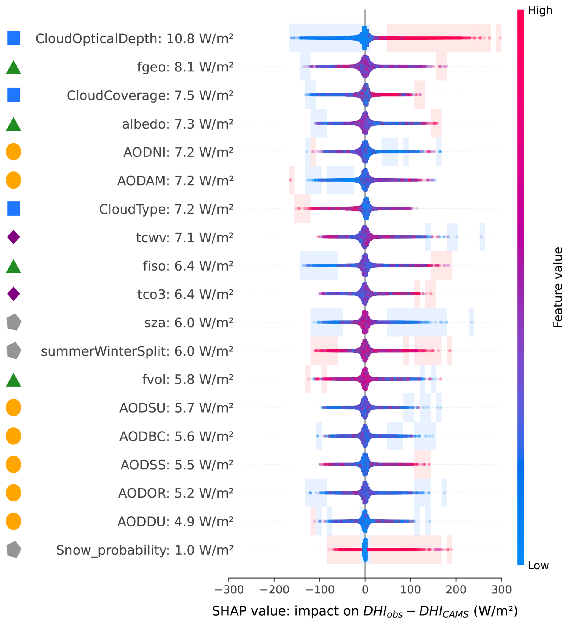
Figure A1SHAP beeswarm plot for the diagnostic DHI residual model defined as DHIobs − DHICRS. Input variables are ordered by their mean absolute SHAP value within the fitted diagnostic models. Each point represents an individual sample model-observation attribution, with the horizontal position showing the SHAP value (impact on the predicted error) and the color indicating the corresponding feature value (blue: smaller than average, red: larger than average). For visualisation purposes, points are vertically displaced within each feature row in regions of high sample density. Shaded regions highlight areas where more than 90 % of the SHAP contributions originate from either larger-than-average (red shading) or smaller-than-average (blue shading) feature values. Symbols on the left denote feature groups (cloud, aerosol, surface, gas, and other variables). Positive SHAP values indicate conditions contributing to CRS DHI underestimation, while negative values indicate CRS DHI overestimation.

Figure A2Mean absolute group-wise SHAP contributions from the diagnostic models, normalised by total DHI, as a function of solar zenith angle. Each curve represents the sum of SHAP values over a feature group. Solar zenith angle is binned using 2.5° intervals over the range 0–80°. The numbers shown above the x axis indicate the number of samples within each solar zenith angle bin.
A2 Beam normal irradiance (BNI)
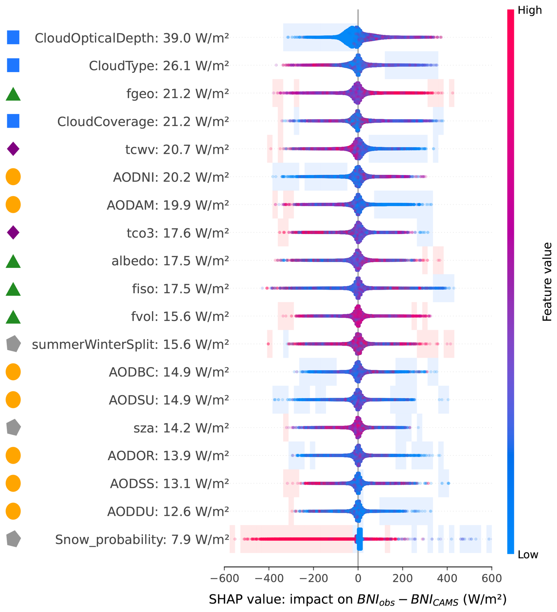
Figure A3SHAP beeswarm plot for the diagnostic BNI residual model defined as BNIobs − BNICRS. Input variables are ordered by their mean absolute SHAP value within the fitted diagnostic models. Each point represents an individual sample model-observation attribution, with the horizontal position showing the SHAP value (impact on the predicted error) and the color indicating the corresponding feature value (blue: smaller than average, red: larger than average). For visualisation purposes, points are vertically displaced within each feature row in regions of high sample density. Shaded regions highlight areas where more than 90 % of the SHAP contributions originate from either larger-than-average (red shading) or smaller-than-average (blue shading) feature values. Symbols on the left denote feature groups (cloud, aerosol, surface, gas, and other variables). Positive SHAP values indicate conditions contributing to CRS BNI underestimation, while negative values indicate CRS BNI overestimation.
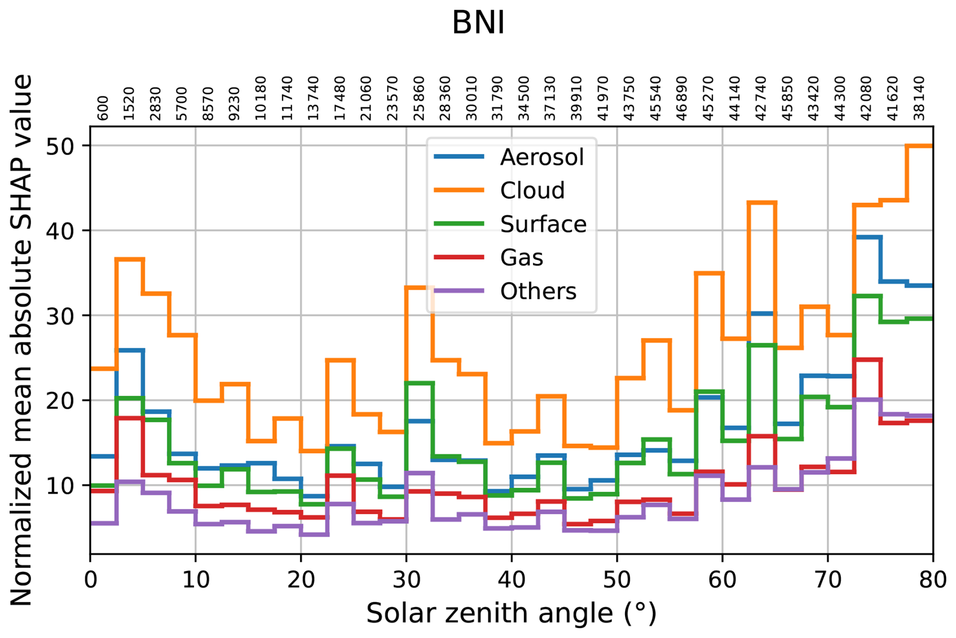
Figure A4Mean absolute group-wise SHAP contributions from the diagnostic models, normalised by total BNI, as a function of solar zenith angle. Each curve represents the sum of SHAP values over a feature group. Solar zenith angle is binned using 2.5° intervals over the range 0–80°. The numbers shown above the x axis indicate the number of samples within each solar zenith angle bin.
Table B1 reports the station-level RMSE changes from the LOSO spatial generalisation sensitivity analysis described in Sect. 3.6.
Table B1Station-level reduction in RMSE (%) in the leave-one-station-out correction experiment. Each station is evaluated using a model fitted on the other 20 stations. Positive values indicate improvement relative to the original CRS product, and negative values indicate deterioration.
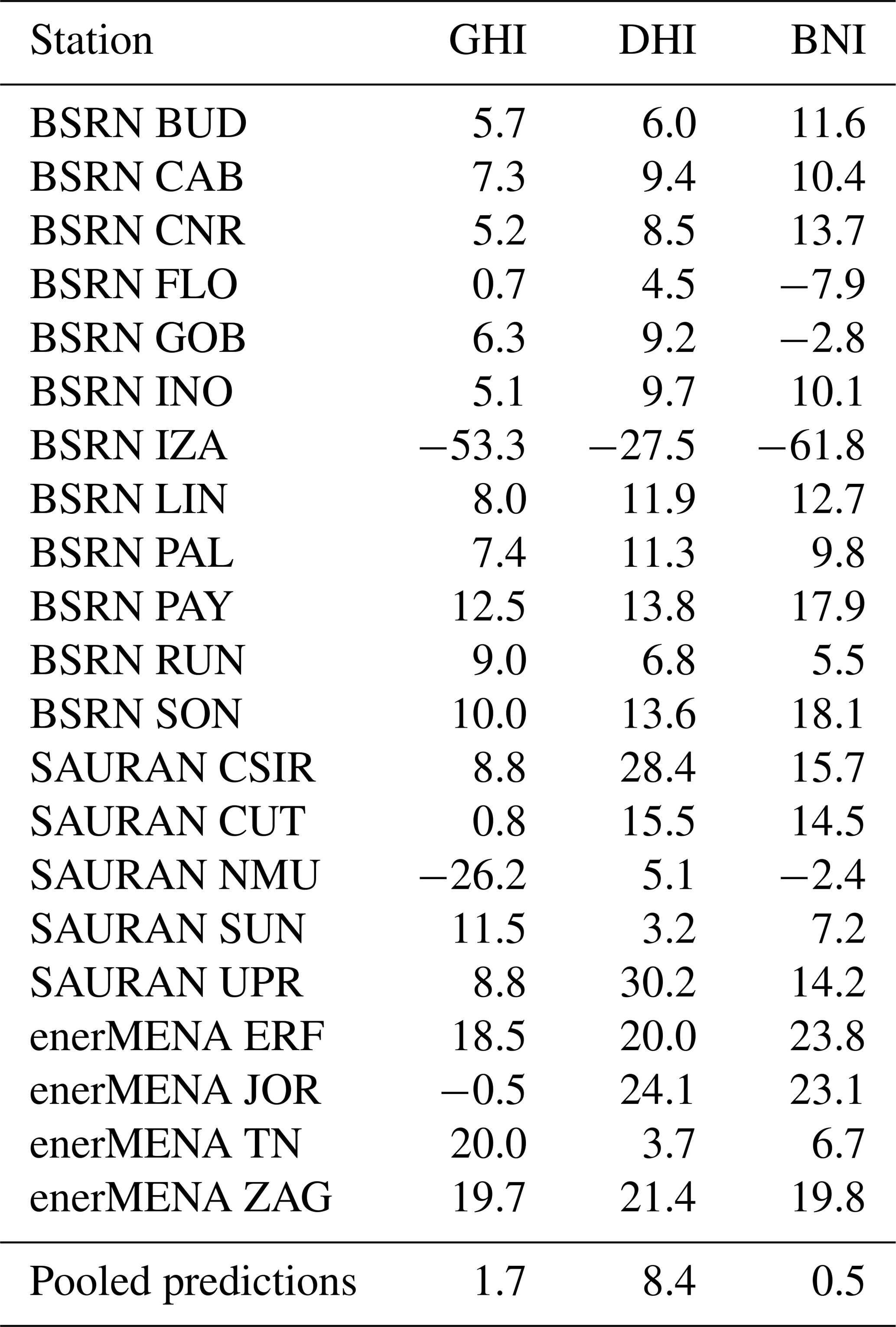
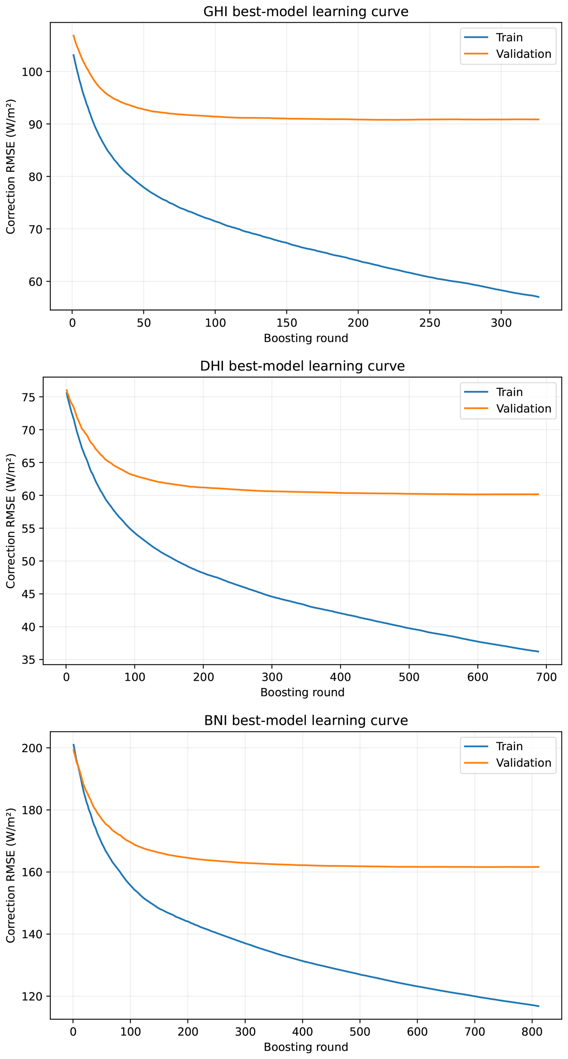
Figure C1Training and validation RMSE as a function of boosting round for the XGBoost residual models for GHI (top), DHI (middle), and BNI (bottom).
Python code to train XGBoost model and run SHAP analysis on solar irradiance data is available at https://github.com/TUT-ISI/SolRadErrorIdentificationAttributionCorrection (last access: 13 November 2026) and archived on Zenodo at https://doi.org/10.5281/zenodo.24194868 (Lipponen, 2026). CRS solar radiation data is publicly available on the CAMS Atmosphere Data Store. The solar irradiance ground observations were prepared and made available to the authors by the CRS development team. All data used in this study is stored at https://tds.webservice-energy.org/thredds/catalog/in-situ.html (Webservice-Energy, 2025). Some of the sites are publicly available (directly downloadable) and others have restricted access (imposed by the data owners). Restricted access data could be requested to the CRS development team.
A.L. designed the methodology, performed the analysis, and wrote the initial draft of the manuscript. J.L. provided the ground-based observational data and contributed to data curation and validation. Y.-M.S.-D., M.S.-H., and A.A. contributed to the planning of the study and to the interpretation of the results. A.L., J.L., Y.-M.S.-D., M.S.-H., and A.A. participated in the scientific discussion, critically reviewed the manuscript, and approved the final version for submission.
The contact author has declared that none of the authors has any competing interests.
Publisher's note: Copernicus Publications remains neutral with regard to jurisdictional claims made in the text, published maps, institutional affiliations, or any other geographical representation in this paper. The authors bear the ultimate responsibility for providing appropriate place names. Views expressed in the text are those of the authors and do not necessarily reflect the views of the publisher.
This research has been supported by the European Commission, HORIZON EUROPE Framework Programme (grant no. 101082125).
This paper was edited by Sandip Dhomse and reviewed by three anonymous referees.
CAMS Radiation Service: Regular Validation Reports, Copernicus Atmosphere Monitoring Service, https://atmosphere.copernicus.eu/supplementary-services (last access: 13 May 2026), 2025. a
Chen, T. and Guestrin, C.: XGBoost: A scalable tree boosting system, in: Proceedings of the 22nd ACM SIGKDD international conference on knowledge discovery and data mining, Association for Computing Machinery, 785–794, https://doi.org/10.1145/2939672.2939785, 2016. a
Copernicus Atmosphere Monitoring Service (CAMS): CAMS solar radiation time‐series, Copernicus Atmosphere Monitoring Service (CAMS) Atmosphere Data Store [data set], https://doi.org/10.24381/5cab0912, 2020. a, b
Copernicus Atmosphere Monitoring Service (CAMS): Supplementary Services, https://atmosphere.copernicus.eu/supplementary-services (last access: 17 July 2026), 2026. a
Dong, J., Zeng, W., Wu, L., Huang, J., Gaiser, T., and Srivastava, A. K.: Enhancing short-term forecasting of daily precipitation using numerical weather prediction bias correcting with XGBoost in different regions of China, Eng. Appl. Artif. Intel., 117, 105579, https://doi.org/10.1016/j.engappai.2022.105579, 2023. a
Driemel, A., Augustine, J., Behrens, K., Colle, S., Cox, C., Cuevas-Agulló, E., Denn, F. M., Duprat, T., Fukuda, M., Grobe, H., Haeffelin, M., Hodges, G., Hyett, N., Ijima, O., Kallis, A., Knap, W., Kustov, V., Long, C. N., Longenecker, D., Lupi, A., Maturilli, M., Mimouni, M., Ntsangwane, L., Ogihara, H., Olano, X., Olefs, M., Omori, M., Passamani, L., Pereira, E. B., Schmithüsen, H., Schumacher, S., Sieger, R., Tamlyn, J., Vogt, R., Vuilleumier, L., Xia, X., Ohmura, A., and König-Langlo, G.: Baseline Surface Radiation Network (BSRN): structure and data description (1992–2017), Earth Syst. Sci. Data, 10, 1491–1501, https://doi.org/10.5194/essd-10-1491-2018, 2018. a
Friedman, J.: Greedy function approximation: A gradient boosting machine, Ann. Stat., 29, 1189–1232, https://doi.org/10.1214/aos/1013203451, 2001. a
Gneiting, T., Raftery, A. E., Westveld III, A. H., and Goldman, T.: Calibrated probabilistic forecasting using ensemble model output statistics and minimum CRPS estimation, Mon. Weather Rev., 133, 1098–1118, https://doi.org/10.1175/MWR2904.1, 2005. a
Gschwind, B., Wald, L., Blanc, P., Lefèvre, M., Schroedter-Homscheidt, M., and Arola, A.: Improving the McClear model estimating the downwelling solar radiation at ground level in cloud-free conditions – McClear-v3, Meteorol. Z., 28, https://doi.org/10.1127/metz/2019/0946, 2019. a
IN-SITU: In-Situ data viewer, https://viewer.webservice-energy.org/in-situ/ (last access: 13 May 2026), 2025. a
Kenny, D. and Fiedler, S.: Which gridded irradiance data is best for modelling photovoltaic power production in Germany?, Sol. Energy, 232, 444–458, https://doi.org/10.1016/j.solener.2021.12.044, 2022. a
Klüser, L., Killius, N., and Gesell, G.: APOLLO_NG – a probabilistic interpretation of the APOLLO legacy for AVHRR heritage channels, Atmos. Meas. Tech., 8, 4155–4170, https://doi.org/10.5194/amt-8-4155-2015, 2015. a
Lefèvre, M., Oumbe, A., Blanc, P., Espinar, B., Gschwind, B., Qu, Z., Wald, L., Schroedter-Homscheidt, M., Hoyer-Klick, C., Arola, A., Benedetti, A., Kaiser, J. W., and Morcrette, J.-J.: McClear: a new model estimating downwelling solar radiation at ground level in clear-sky conditions, Atmos. Meas. Tech., 6, 2403–2418, https://doi.org/10.5194/amt-6-2403-2013, 2013. a, b
Lezaca Galeano, J. E., Saint-Drenan, Y.-M., and Schroedter-Homscheidt, M.: A Probabilistic Approach to Quantify the Uncertainty of the 1 Min Irradiance Estimates from the Copernicus Atmosphere Monitoring Service (CAMS) Radiation Service, Solar RRL, 9, e202500568, https://doi.org/10.1002/solr.202500568, 2025. a
Lipponen, A.: Machine-learning-based approach for solar radiation model prediction error identification, attribution and correction script, Version v1.0.0, Zenodo [computer software], https://doi.org/10.5281/zenodo.24194868, 2026. a
Lipponen, A., Kolehmainen, V., Romakkaniemi, S., and Kokkola, H.: Correction of approximation errors with Random Forests applied to modelling of cloud droplet formation, Geosci. Model Dev., 6, 2087–2098, https://doi.org/10.5194/gmd-6-2087-2013, 2013. a
Lipponen, A., Huttunen, J. M., Romakkaniemi, S., Kokkola, H., and Kolehmainen, V.: Correction of model reduction errors in simulations, SIAM J. Sci. Comput., 40, B305–B327, 2018. a
Lipponen, A., Kolehmainen, V., Kolmonen, P., Kukkurainen, A., Mielonen, T., Sabater, N., Sogacheva, L., Virtanen, T. H., and Arola, A.: Model-enforced post-process correction of satellite aerosol retrievals, Atmos. Meas. Tech., 14, 2981–2992, https://doi.org/10.5194/amt-14-2981-2021, 2021. a
Long, C. and Dutton, E.: BSRN Global Network recommended QC tests, V2.0, Tech. rep., Baseline Surface Radiation Network, https://epic.awi.de/id/eprint/30083/1/BSRN_recommended_QC_tests_V2.pdf (last access: 13 May 2026), 2022. a
Lundberg, S. M. and Lee, S.-I.: A unified approach to interpreting model predictions, Advances in neural information processing systems, Vol. 30, https://proceedings.neurips.cc/paper_files/paper/2017/file/8a20a8621978632d76c43dfd28b67767-Paper.pdf (last access: 13 May 2026), 2017. a, b, c
Lundberg, S. M., Erion, G., Chen, H., DeGrave, A., Prutkin, J. M., Nair, B., Katz, R., Himmelfarb, J., Bansal, N., and Lee, S.-I.: From local explanations to global understanding with explainable AI for trees, Nature Machine Intelligence, 2, 56–67, https://doi.org/10.1038/s42256-019-0138-9, 2020. a
Ma, J., Yu, Z., Qu, Y., Xu, J., and Cao, Y.: Application of the XGBoost machine learning method in PM2.5 prediction: A case study of Shanghai, Aerosol Air Qual. Res., 20, 128–138, https://doi.org/10.4209/aaqr.2019.08.0408, 2020. a
Mabasa, B., Lysko, M. D., and Moloi, S. J.: Validating hourly satellite based and reanalysis based global horizontal irradiance datasets over South Africa, Geomatics, 1, 429–449, https://doi.org/10.3390/geomatics1040025, 2021. a
Mardaljevic, J., Brembilla, E., and Eames, M.: Daylight solar radiation AMY data derived from satellite remote sensing: Validation against ground measurements and comparison with TMYs, Build. Serv. Eng. Res. T., 46, 653–691, https://doi.org/10.1177/01436244251335160, 2025. a
Muschinski, T., Mayr, G. J., Zeileis, A., and Simon, T.: Robust weather-adaptive post-processing using model output statistics random forests, Nonlin. Processes Geophys., 30, 503–514, https://doi.org/10.5194/npg-30-503-2023, 2023. a
Myers, D. R.: Solar radiation modeling and measurements for renewable energy applications: data and model quality, Energy, 30, 1517–1531, https://doi.org/10.1016/j.energy.2004.04.034, 2005. a
Natekin, A. and Knoll, A.: Gradient boosting machines, a tutorial, Front. Neurorobotics, 7, 21, https://doi.org/10.3389/fnbot.2013.00021, 2013. a
Peuch, V.-H., Engelen, R., Rixen, M., Dee, D., Flemming, J., Suttie, M., Ades, M., Agustí-Panareda, A., Ananasso, C., Andersson, E., Armstrong, D., Barré, J., Bousserez, N., Dominguez, J. J., Garrigues, S., Inness, A., Jones, L., Kipling, Z., Letertre-Danczak, J., Parrington, M., Razinger, M., Ribas, R., Vermoote, S., Yang, X., Simmons, A., Garcés de Marcilla, J., and Thépaut, J.-N.: The Copernicus Atmosphere Monitoring Service: From research to operations, B. Am. Meteorol. Soc., 103, E2650–E2668, https://doi.org/10.1175/BAMS-D-21-0314.1, 2022. a, b
Qu, Z., Oumbe, A., Blanc, P., Espinar, B., Gesell, G., Gschwind, B., Klüser, L., Lefèvre, M., Saboret, L., Schroedter-Homscheidt, M., and Wald, L.: Fast radiative transfer parameterisation for assessing the surface solar irradiance: The Heliosat-4 method, Meteorol. Z., 26, 33–57, https://doi.org/10.1127/metz/2016/0781, 2017. a, b
Riise, H. N., Nygard, M. M., Aarseth, B. L., Dobler, A., and Berge, E.: Benchmark of estimated solar irradiance data at high latitude locations, Sol. Energy, 282, 112975, https://doi.org/10.1016/j.solener.2024.112975, 2024. a
SAURAN: Southern African Universities Radiometric Network, https://sauran.ac.za/ (last access: 13 May 2026), 2025. a
Schroedter-Homscheidt, M., Azam, F., Betcke, J., Hanrieder, N., Lefevre, M., Saboret, L., and Saint-Drenan, Y.-M.: Surface solar irradiation retrieval from MSG/SEVIRI based on APOLLO Next Generation and HELIOSAT-4 methods, Meteorol. Z., 31, 455–476, https://doi.org/10.1127/metz/2022/1132, 2022. a, b, c
Schüler, D., Wilbert, S., Geuder, N., Affolter, R., Wolfertstetter, F., Prahl, C., Röger, M., Schroedter-Homscheidt, M., Abdellatif, G., Guizani, A. A., Balghouthi, M., Khalil, A., Mezrhab, A., Al-Salaymeh, A., Yassaa, N., Chellali, F., Draou, D., Blanc, P., Dubranna, J., and Sabry, O. M. K.: The enerMENA meteorological network – Solar radiation measurements in the MENA region, AIP Conf. Proc., 1734, 150008, https://doi.org/10.1063/1.4949240, 2016. a
Shapley, L.: A value for n-person games, in: Contributions to the Theory of Games AM-28, Princeton University Press, II, 307–318, https://doi.org/10.1515/9781400881970-018, 1953. a
Urraca, R., Trentmann, J., Pfeifroth, U., and Gobron, N.: Can satellite products monitor solar brightening in Europe?, Remote Sens. Environ., 315, 114472, https://doi.org/10.1016/j.rse.2024.114472, 2024. a
Webservice-Energy: Solar Irradiance ground observations THREDDS Catalog, https://tds.webservice-energy.org/thredds/catalog/in-situ.html (last access: 13 May 2026), 2025. a, b
Wild, M., Folini, D., Schär, C., Loeb, N., Dutton, E. G., and König-Langlo, G.: The global energy balance from a surface perspective, Clim. Dynam., 40, 3107–3134, https://doi.org/10.1007/s00382-012-1569-8, 2013. a
Zhen, J., Mao, D., Shen, Z., Zhao, D., Xu, Y., Wang, J., Jia, M., Wang, Z., and Ren, C.: Performance of xgboost ensemble learning algorithm for mangrove species classification with multisource spaceborne remote sensing data, Journal of Remote Sensing, 4, 0146, https://doi.org/10.34133/remotesensing.0146, 2024. a
- Abstract
- Introduction
- Materials and methods
- Results
- Conclusions
- Appendix A: Supplementary SHAP analysis
- Appendix B: Leave-one-station-out correction results
- Appendix C: Model learning curves
- Code and data availability
- Author contributions
- Competing interests
- Disclaimer
- Financial support
- Review statement
- References
- Abstract
- Introduction
- Materials and methods
- Results
- Conclusions
- Appendix A: Supplementary SHAP analysis
- Appendix B: Leave-one-station-out correction results
- Appendix C: Model learning curves
- Code and data availability
- Author contributions
- Competing interests
- Disclaimer
- Financial support
- Review statement
- References