A new method for estimating cloud optical depth from photovoltaic power measurements

A new method was developed to estimate the cloud optical depth (τ_c) from photovoltaic (PV) power measurements under overcast sky conditions. It is a fully physical method utilizing directly PV power measurements. It exploits the recent advances and real-time availability at global scale of aerosol properties, downwelling shortwave irradiance and its direct and diffuse components received at ground level under clear-sky conditions and ground albedo, altogether provided by the Copernicus Atmosphere Monitoring Service (CAMS) radiation service. In addition to CAMS data, wind speed and air temperature from European Centre for Medium-Range Weather Forecasts twentieth century reanalysis ERA5 products are also used as inputs. The τ_c estimates have been compared to different data sources of τ_c retrievals at four experimental PV sites located in various climates. When compared to τ_c retrieved from ground-based pyranometer measurements serving as reference, the correlation coefficient is greater than 0.97. The bias ranges between −3 and 4, i.e., −8 % and 14 % in relative value. The root mean square error (RMSE) lies in the interval [3,8] ([9,21] % in relative value). When compared to satellite-based retrievals from Meteosat Second Generation and Moderate Resolution Imaging Spectroradiometer, both relative errors become comprehensively greater. Nevertheless, our method remarkably reduces the relative bias and RMSE, by up to 10 % and 20 % respectively, compared to the existing state-of-the-art approach. This work demonstrates the accuracy of the method and clearly shows its great potential use whenever PV power measurements are available.

1 Introduction

Clouds are a key component in weather and climate, influencing both incoming solar shortwave radiation and outgoing thermal radiation. During recent years, electricity production using solar photovoltaic (PV) panels has grown rapidly worldwide. As the number of PV installations continues to grow, it is apparent that the network of PV installations constitutes a highly interesting, potential new source of cloud information. From a meteorological perspective, there is a connection between solar electricity production also called PV production or PV power output, solar radiation and prevailing cloud conditions (see, e.g., Stylianou et al., 2020). When the meteorological conditions are known, the electricity production of a known PV system can be accurately modeled (e.g., Böök et al., 2020). Here, the cloud optical depth (τ_c) is of central importance, as it governs how incoming solar radiation attenuates due to clouds.

In a previous study (Wandji Nyamsi and Lindfors, 2024), we developed and validated a method for detecting clear-sky periods from PV power output data, showing performance similar to that of methods based on measurements of the broadband solar irradiance on a horizontal surface at the ground level, here abbreviated as SSI. In the present study, we focus on cloudy conditions, with the aim to develop an approach for estimating τ_c from PV power output data.

τ_c has been widely retrieved by the means of satellite-based measurements (e.g., Wielicki and Parker, 1992; Platnick et al., 2017), providing extensive spatial coverage needed for studies on continental or global scales. For instruments aboard polar orbiting platforms, such as the Moderate Resolution Imaging Spectroradiometer (MODIS), the temporal coverage is limited, however, as measurements for a specific location only are available at overpass time. Furthermore, satellite-based τ_c may present uncertainties and inhomogeneities which are not yet fully understood (Zeng et al., 2012; Aebi et al., 2020).

Methodologies for retrieving τ_c from ground-based SSI measurements have been proposed in the literature (e.g., Leontyeva and Stamnes, 1994; Barnard and Long, 2004; Qiu, 2006; Aebi et al., 2020). Among them, Barnard and Long (2004) have developed an empirical relationship to determine τ_c for liquid water clouds under overcast sky conditions using only SSI measurements, ground albedo, denoted ρ_g, and solar zenithal angle, denoted θ_S, and accurate “clear sky” SSI. Their empirical formula has been built on the robust results from transmission-based algorithms using spectral irradiances (Min and Harrison, 1996). The medians of the Min and Harrison's algorithm-derived and empirically derived distributions agree within less than 10 % over a wide spatial coverage of locations. SSI measurements offer long time series and noticeable worldwide spatial coverage. SSI is also called downwelling solar irradiance at the surface, downwelling shortwave flux at the surface or simply global SSI, denoted G. G is the sum of its direct component, denoted B, that is, flux coming from the direction of the sun on a horizontal surface, and the diffuse component, denoted D, that is, the flux accounting all remaining directions from the sky vault so that G = B + D.

In the context of estimating τ_c from PV power output, Barry et al. (2023) presented a pioneering study based on two measurement campaigns in the Allgäu region in Germany. They made first tests on estimating τ_c for liquid water clouds from PV output, with reasonable results compared to satellite-retrieved τ_c. Their approach is rather detailed, however, including building a look-up-table (LUT) for each 15 min time interval of interest and utilizing ancillary ground-based measurements of aerosol properties at the given location. In addition, it is also required to convert PV output into solar irradiance from which τ_c can be retrieved yielding similarly to a broadband pyranometer approach as mentioned earlier. A similar synergy of radiative transfer modelling coupled with PV power measurements has been utilized earlier for retrieving aerosol optical thickness (Lolli, 2021). The present study aims at building a more general approach, utilizing commonly available data sources so that the method is applicable at any location of interest, where suitable PV power output data are available. The method exploits the PV model of our previous work (Wandji Nyamsi and Lindfors, 2024) and libRadtran radiative transfer modelling (Emde et al., 2016; Mayer and Kylling, 2005) in combination with aerosol properties, ground albedo and cloud-free SSI components provided by Copernicus Atmosphere Monitoring Service (CAMS) radiation service (Qu et al., 2017; Schroedter-Homscheidt et al., 2022).

The paper is organized as follows. In Sect. 2, a detailed description of all data used in this study is given. Then, a procedure to select overcast sky conditions is presented in Sect. 3. The developed method of this study estimating τ_c directly from PV power measurements is presented in a detailed manner in Sect 4. The performance of the proposed method is evaluated at four experimental PV sites located in various climatic zones by comparing estimated τ_c from PV power measurements against different data sources of τ_c retrievals. The results of comparisons are given and discussed in Sect. 5 as well as possible explanations for the discrepancies between τ_c retrievals. Eventually, the conclusions and brief outlook are given in Sect. 6.

2 Data used in this study

All data used in this study can be freely collected through public sources available online or can be provided by the authors upon request. Details on how to collect them are mentioned in this section and are given in the section “Data availability”.

2.1 Irradiance and PV power measurements

Highly maintained ground-based sites carrying out PV power measurements fulfilling three main constraints have been selected for this study. The first one is that PV power measurements should be collocated with SSI measurements with a maximum distance of 1 km. The second one is that the temporal resolution of both collocated PV and SSI measurements should be of 1 min which is also the temporal resolution for all modelled data. The third constraint is that the temporal period of measurements should cover at least four full years. After searching, we found four PV sites over Europe covering various climates meeting those criteria: Helsinki and Kuopio of the Finnish Meteorological Institute (FMI), one site in The Netherlands, obtained in context of the Solar Forecasting and Smart Grids (SF&SG) research project (Visser et al., 2022) and one site monitored by the Laboratory for Photovoltaic Systems (PV Lab) of Bern University of Applied Sciences BFH in Burgdorf, Switzerland.

Ground-based SSI measurements were collected for the same sites. For Helsinki, Kuopio and Burgdorf, SSI is measured in the immediate vicinity of the PV systems. For the Dutch site, the closest PV site (originally identified by “ID023” in the metadata file and hereafter named “Cabauw–ID023”) to ground-based station Cabauw has been selected. The station Cabauw belongs to the Baseline Surface Radiation Network (BSRN, Ohmura et al., 1998; Mol et al., 2023) providing high-quality SSI measurement data.

Table 1 lists the PV sites used with their respective name, country, source, geographical coordinates, temporal period of measurements (used also for all modelled data) and specifications of installed PV systems. It also reports the corresponding Köppen–Geiger climate type for each station according to Peel et al. (2007). All PV systems used in this study are on a flat roof with fixed tilt orientation and their module material is polycrystalline silicon, the most popular material type in the PV market except at the Swiss site having monocrystalline silicon solar cells. For all PV systems, measured electrical power output is collected under the form of alternating current (AC) power data, which is more commonly available. AC power data is induced by the inverter having its own characteristics and behavior. For the Swiss site, the nominal capacity of system found in the metadata file was seen unreliable. Therefore, a scaling factor has been computed between measured and estimated (using the unreliable value) PV power based on few visually selected clear-sky days. The scaling factor has then been applied to the unreliable nominal capacity to derive a more plausible nominal capacity which is reported in Table 1.

Table 1 Description of ground-based PV sites used for this study, ordered from the northernmost station to the southernmost one.

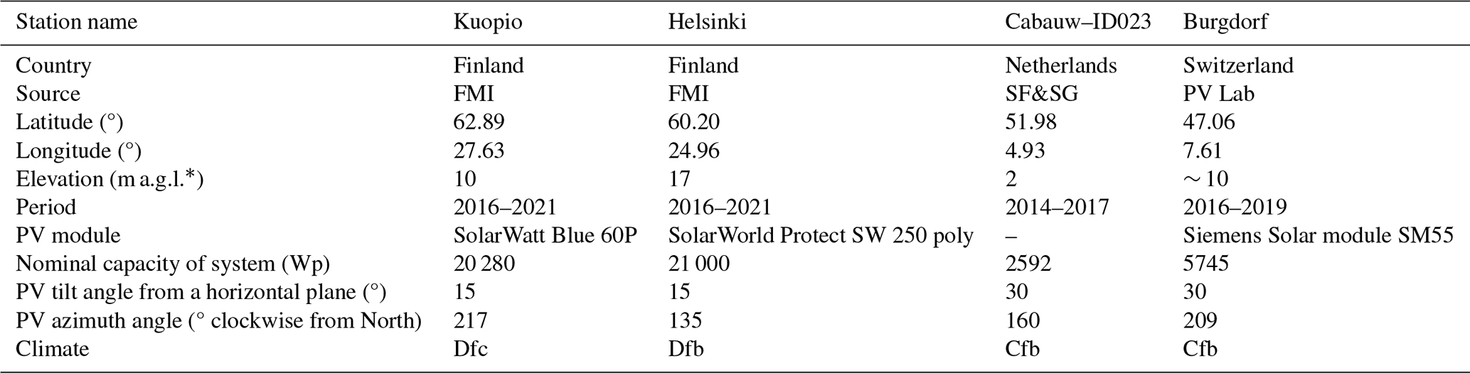
^* a.g.l.: above the ground level. Dfc: continental climate with no dry season and cold summer. Dfb: continental climate with no dry season and warm summer. Cfb: temperate climate with no dry season and warm summer.

Table 2 reports detailed information for collocated SSI stations. For Finnish sites, all relevant measurements are described in detailed manner in Karhu et al. (2025) and are freely accessible and downloadable through the website https://doi.org/10.57707/fmi-b2share.c7b3ec9f19324a6497639d6d8c0cde84 (Karhu and Lindfors, 2025). For Cabauw–ID023, G and PV power measurements can be downloaded freely from the website https://bsrn.awi.de (last access: 1 March 2025; Alfred-Wegener-Institute, 2022) and https://doi.org/10.5281/zenodo.10953360 (Visser et al., 2022) respectively. The corresponding best quality-controlled PV power measurements are selected from the file named filtered_pv_power_measurements_ac.csv, https://zenodo.org/records/10953360/files/filtered_pv_power_measurements_ac.csv?download=1 (last access: 1 March 2025).

Table 2 Collocated SSI station, measurement instruments used at each station with their specifications.

2.2 CAMS radiation service products

PV output depends primarily on the prevailing solar radiation conditions and weather observations, both of which depend on atmospheric conditions. In that sense, SSI data and atmospheric conditions are properly used as inputs to the PV model (Wandji Nyamsi and Lindfors, 2024; Wandji et al., 2025). The CAMS radiation service (Schroedter-Homscheidt, 2019) makes use of the Heliosat-4 method (Qu et al., 2017; Schroedter-Homscheidt et al., 2022) built on LUTs established on the basis of the radiative transfer model (RTM) libRadtran (Emde et al., 2016; Mayer and Kylling, 2005) with the improved Kato et al. (1999) approach (kato2andwandji as named in libRadtran, Wandji Nyamsi et al., 2014, 2015a). It is constituted of two models: (1) the McClear model (Lefèvre et al., 2013; Wandji Nyamsi et al., 2023a) estimating the irradiances under clear-sky conditions and (2) the McCloud model estimating the attenuation due only to clouds. CAMS radiation service utilizes datasets from various databases such as the CAMS and NASA's MODIS observations describing the atmospheric state and ground type as well as cloud properties derived from 15 min Meteosat Second Generation (MSG) satellite images using an adapted Advanced Very High-Resolution Radiometer (AVHRR) Processing scheme Over cLoud, Land, and Ocean Next Generation (APOLLO_NG) algorithm (Kriebel et al., 2003; Klüser et al., 2015). With the geographic coordinates at any location over Africa, Atlantic Ocean, Eastern part of South America, Europe, Middle East, it delivers very rapidly a time series of G, D, B or the direct component at normal incidence B_N under both clear-sky and all-sky conditions at the ground level as well as extraterrestrial irradiance on a horizontal plane, denoted E_O, for any period from 2004 until 2 d ago with different temporal summarization (1 min, 15 min, 60 min, 1 d and 1 month).

CAMS products are freely accessible by machine-to-machine calls to the Web service CAMS radiation on the SoDa Service (Gschwind et al., 2006, https://www.soda-pro.com/, last access: 1 March 2025) or manually through a web interface. In the verbose mode, CAMS radiation service restitutes 1 min values of readings from CAMS interpolated in space and time, namely, total column of water vapor (TWV) and ozone (TOC) and aerosol optical depth (AOD) at 550 nm, denoted AOD₅₅₀. It also contains 1 min values of θ_S, computed with the SG2 algorithm (Blanc and Wald, 2012), ρ_g, τ_c at 600 nm (${\mathit{\tau }}_{\mathrm{c}}^{\mathrm{CAMS}}$), cloud fraction (CF^CAMS), and cloud phase (CP^CAMS) for the location under concern. This mode was conveniently utilized for the collection of CAMS products for the entire measurement period.

Among selected CAMS products, G_clear, D_clear, B_{N_clear} (with subscript clear referring to clear-sky conditions), E_O, θ_S, ρ_g are altogether used for PV power computations under clear-sky conditions while ${\mathit{\tau }}_{\mathrm{c}}^{\mathrm{CAMS}}$, CF^CAMS and CP^CAMS are appropriately exploited for comparison purposes between τ_c retrievals. CAMS Radiation Service v4.6 was used here. The respective products have been downloaded from the website https://www.soda-pro.com/web-services/radiation/cams-radiation-service (last access: 1 March 2025) after registration. It should be noted that while CAMS cloud properties are only available for location within the MSG and HIMAWARI field of view (FOV), CAMS clear-sky products are available at any location over the globe and any time after 2003 through McClear service similarly accessing as CAMS radiation service.

2.3 ECMWF wind speed and air temperature

Wind speed and air temperature, both having a noticeable spatial and temporal variation, play a crucial role in PV system performance. More specifically, both wind speed and air temperature are included because of their effect on the temperature of the PV modules (see Eq. A10 of the PV model explicitly given in Appendix A) and because the module temperature influences the relative efficiency of the PV system (warmer temperatures give less efficient PV systems; see Eq. A13 of the PV model explicitly given in Appendix A) Here, the ERA5 reanalysis of the European Centre for Medium-range Weather Forecasts (ECMWF) is utilized. ERA5 provides a consistent and globally complete data set that has been produced by combining model data with worldwide observations (Hersbach et al., 2023). Outputs are available at an hourly temporal resolution covering the period from 1940 onwards at a spatial resolution of 0.25° latitude × 0.25° longitude (approximately 30 km).

In this study, we used the 10 m wind speed (ws) and air temperature at 2 m (T_air) from ERA5. The hourly data was resampled in time to the closest pixel of each station by linear interpolation to derive 1 min data. The data derived from this latter procedure are also used for τ_c estimates as explained later. The ERA5 products have been downloaded from the website https://cds.climate.copernicus.eu/datasets/reanalysis-era5-single-levels?tab=download (last access: 1 March 2025).

2.4 MODIS cloud products

The MODIS level-2 cloud products, namely MOD06_L2 and MYD06_L2 data collected from the Terra and Aqua platforms, respectively, are instantaneous level-2 satellite atmosphere datasets based on NASA's MODIS observations under both daytime and nighttime conditions. MODIS instruments fly onboard both Terra (morning overpass) and Aqua (afternoon overpass) satellites providing information for cloudy pixels over both land and ocean. In this level-2 product, the cloud property retrievals are composed of cloud optical and physical parameters with spatial resolution of either 1 or 5 km (at nadir). Selected cloud data from the given location and at the exact satellite overpass time at 1 km spatial resolution during the daytime are τ_c at 0.66 µm over land (hereinafter ${\mathit{\tau }}_{\mathrm{c}}^{\mathrm{MODIS}}$), cloud phase (hereinafter CP^MODIS), distance of the pixel used to compute cloud fraction (hereinafter CF^MODIS). CF^MODIS are essentially computed within a circle with a diameter of 20 km as the ratio of confidently and probably cloudy pixels to all determined pixels including probably clear, or confidently clear pixels (Pincus et al., 2023). ${\mathit{\tau }}_{\mathrm{c}}^{\mathrm{MODIS}}$ serving as reference is used for performing comparisons with τ_c retrieved from PV power measurements. CF^MODIS and CP^MODIS are used for overcast sky selection and cloud phase discrimination purposes respectively. Cloud products used are products of Collection 6/6.1 Level-2 MOD06/MYD06 Product (Platnick et al., 2017). Relevant MODIS data are downloadable at https://ladsweb.modaps.eosdis.nasa.gov/missions-and-measurements/products/MOD06_L2 (last access: 1 March 2025) and https://ladsweb.modaps.eosdis.nasa.gov/missions-and-measurements/products/MYD06_L2 (last access: 1 March 2025).

2.5 Calibrated clear-sky PV power and global SSI time series

The selection of periods under overcast sky conditions and then estimating τ_c from PV power measurements requires clear-sky PV power time series with high accuracy. For doing so, the methodology described by Wandji Nyamsi and Lindfors (2024) has been applied. In brief, for a given location and over the relevant measurement period, 1 min values of G_clear, D_clear, B_{N_clear}, E_O, θ_S, ρ_g were collected from the CAMS and ws and T_air from ERA5 (see in Sect. 2.2 and 2.3). These collected time series are inputs to the designed PV model by Wandji Nyamsi and Lindfors (2024) in order to produce time series of clear-sky PV power. All necessary equations for the PV model are explicitly given in Appendix A. The designed PV model, hereafter simply called PV model, is also conveniently used in the rest of this paper.

Both PV power measurements and time series of clear-sky PV power are used in the clear sky detection methodology developed by Wandji Nyamsi and Lindfors (2024) providing a set of clear-sky minutes over the measurement period. Then, both measurements and clear-sky time series of PV power at those detected clear-sky minutes are grouped on a monthly basis to determine a monthly calibration factor. The coefficient is then applied on the initial full time series of clear sky PV power yielding calibrated time series of clear-sky PV power. Hereafter, P^m and $P_{\mathrm{clear}}^{\mathrm{e}}$ denote measured PV power and calibrated clear sky estimates of PV power respectively. The superscripts m and e indicate measured and estimated values respectively. We assume that a clear-sky instant detected by analyzing PV power measurements is also clear-sky for the irradiance measurements. The time series of measured G and G_clear are exploited at the previously detected clear-sky minutes to compute a calibration factor which is then applied on original time series of G_clear to produce a continuous calibrated clear sky G noted $G_{\mathrm{clear}}^{\mathrm{CAMS}}$. This latter will be one of the inputs of Barnard and Long (2004)'s formula to determine τ_c as exploited in Sect. 5.1.

3 Algorithm for selecting periods under overcast sky conditions

τ_c retrievals are typically operated under overcast sky conditions (Barnard and Long, 2004; Barnard et al., 2008). Such sky conditions as well as cloud type at ground level are most reliably identified with hemispheric sky cameras based on techniques analyzing all-sky images (Long et al., 2006; Wacker et al., 2015; Gueymard et al., 2019). From these techniques, a cloud parameter namely CF is determined for an effective 160° FOV. Overcast sky conditions occurs when CF is greater than 0.95 (Wandji Nyamsi et al., 2023b, 2024).

In addition, cloud type is further intuitively used to assign a CP. A reliable CP is a crucial element in the accurate τ_c retrievals. Three CP are often produced when analyzing clouds: liquid water phase or simply water phase, ice phase and mixed (water and ice)-phase. However, accurate distinction between phases beyond just water and ice remains a challenging task (Korolev et al., 2017; Mayer et al., 2024). This is also seen with passive sensors aboard geostationary satellites observing clouds from space. For instance, MODIS categorizes a cloudy pixel as only water, ice or undetermined phase (Platnick et al., 2017). Considering this challenging issue and substantial errors which may be caused by an incorrect cloud phase detection, this study will be focused on two cloud phases either water or ice phase.

Unfortunately, such cloud parameters are not available at studied locations. Because the ultimate idea is to carry out the best possible selection of both overcast sky periods and cloud phase for possibly any operational use, the proposed algorithm here combines PV power measurements and satellite-based CF and CP. The main reason for this combination is that (1) PV power measurements have a limited FOV depending on PV geometric orientation (i.e., namely the PV tilt angle noted θ_T, the PV azimuth angle noted Φ_T) and (2) the much wider FOV of a satellite can complement the PV FOV in order to reach a larger FOV.

To do so, every N-min time window centered at the instantaneous satellite observation time specifically between sunrise and sunset is investigated to categorize the time window as overcast or not. Three filters have been applied as follows in order to retain reliable overcast sky conditions.

Firstly, with PV power measurements, the proposed algorithm computes three statistical parameters that describe the smoothness and magnitude of P^m with respect to $P_{\mathrm{clear}}^{\mathrm{e}}$ over a given N-min time window. The first filter looks at the physical quantity accounting for the attenuation due only to clouds on PV power, called PV clear-sky index, denoted $K_{\mathrm{c}}^{\mathrm{PV}}$, the ratio of the actual PV power output to its theoretical power output under clear-sky conditions (Engerer and Mills, 2014). When using PV power measurements, the index is mathematically defined as $K_{\mathrm{c}\mathrm{\_}\mathrm{meas}}^{\mathrm{PV}}=\frac{P^{\mathrm{m}}}{P_{\mathrm{clear}}^{\mathrm{e}}}$. $K_{\mathrm{c}\mathrm{\_}\mathrm{meas}}^{\mathrm{PV}}$ serves as an indicator of the deviation between P^m and $P_{\mathrm{c}}^{\mathrm{e}}$. It exhibits insights into the presence of clouds in the sky. $K_{\mathrm{c}}^{\mathrm{PV}}$ close to 1 would indicate an atmosphere under clear sky conditions while $K_{\mathrm{c}}^{\mathrm{PV}}$ quite low would indicate an atmosphere under overcast sky conditions. Therefore, as a first filter, the mean of $K_{\mathrm{c}\mathrm{\_}\mathrm{meas}}^{\mathrm{PV}}$ over the N-min time window should be lower than a certain threshold. It is mathematically formulated as follows: $\stackrel{\mathrm{‾}}{K_{\mathrm{c}\mathrm{\_}\mathrm{meas}}^{\mathrm{PV}}}=\frac{{\sum }_{i=\mathrm{1}}^N{K}_{\mathrm{c}\mathrm{\_}{\mathrm{meas}}_i}^{\mathrm{PV}}}{N}\le {\mathit{\delta }}_{\mathrm{1}}$ where $K_{\mathrm{c}\mathrm{\_}{\mathrm{meas}}_i}^{\mathrm{PV}}$ is $K_{\mathrm{c}\mathrm{\_}\mathrm{meas}}^{\mathrm{PV}}$ at ith minute of the N-min time window.

The second filter scrutinizes the temporal fluctuation of $K_{c\mathit{\_}meas}^{\mathrm{PV}}$. In case of overcast sky situations, the sky should be overcast for a long period. Looking at this would avoid cases of broken clouds or significant spatial heterogeneity around the given location if ergodicity is assumed. Therefore, as a second constraint, the standard deviation should be lower than a certain limit to distinguish between overcast and partly cloudy sky conditions. This is mathematically formulated as $\mathit{\sigma }=\sqrt{\frac{{\sum }_{i=\mathrm{1}}^{N-\mathrm{1}}{\left(K_{\mathrm{c}\mathrm{\_}{\mathrm{meas}}_i}^{\mathrm{PV}}-\stackrel{\mathrm{‾}}{K_{\mathrm{c}\mathrm{\_}\mathrm{meas}}^{\mathrm{PV}}}\right)}^{\mathrm{2}}}{N-\mathrm{1}}}\le {\mathit{\delta }}_{\mathrm{2}}$. As a final constraint and third filter based on satellite data, CF^Satellite should be greater than 0.90 where the satellite sensor can be either the one related to CAMS or MODIS data.

Only N-min series passing simultaneously and successfully all three filters were categorized as under overcast sky conditions. Each minute within such series is also categorized as under overcast sky conditions. For this study, thresholds δ₁ and δ₂ are empirically established and set to 0.4 and 0.1 respectively for 15 min series. Once the overcast sky period is detected, corresponding CP^Satellite is used further in the τ_c retrievals.

4 Estimating τ_c directly from PV power measurements

The concept underlying the proposed method aims at fulfilling four main constraints: (1) the method can be universally applicable where P^m are available but other ancillary measurements (e.g., aerosol properties) are not, (2) it can be easily implemented for routine calculations of τ_c; (3) it should be computationally rapid while retaining the suppleness of using P^m and (4) τ_c estimates should be sufficiently accurate at any location and any time. In addition, the method should not depend on empirical relationships for deriving τ_c. Therefore, to achieve this objective, the development of the method is based on the combination of libRadtran and PV model, both helping to build $K_{\mathrm{c}}^{\mathrm{PV}}$–LUT for inferring τ_c. The use of both models is described and explained in a detailed manner later.

4.1 Radiative transfer simulations with libRadtran 2.0.6

As previously mentioned, PV output in all-sky conditions relies also on the prevailing solar radiation conditions which are determined based on atmospheric conditions. libRadtran is a convenient tool used here for estimating SSI. It simulates the radiative transfer in the Earth's atmosphere under both clear-sky and cloudy atmospheres for various wavelengths. An atmospheric state in clear-sky conditions is a combination of θ_s, ρ_g, TOC, TWC, AOD₅₅₀, vertical profile of temperature, pressure, density, and volume mixing ratio for gases as a function of altitude, aerosol type, and the elevation of the ground above sea level. In cloudy atmosphere, cloud properties, namely phase, effective radius of water droplet and ice crystals, τ_c at 550 nm (τ_c,550), cloud base height and thickness, are added to the variables of the clear-sky atmospheric state.

All radiative transfer simulations (RTS) were performed with libRadtran 2.0.6 (Emde et al., 2016; Mayer and Kylling, 2005). The most improved version of spectral resolution of Kato et al. (1999) approach was selected for band parameterization of absorption cross sections. This latter allows to produce irradiance in 32 wavelength intervals, hereafter named “Kato bands” (KBs) over the shortwave solar spectrum, from 240 to 4606 nm therefore defining the wavelength range for all RTS. A 1D plane-parallel atmosphere was assumed and the DISORT 2.0 (discrete ordinate technique) solver (Stamnes et al., 1988, 2000) with 16 streams was selected to solve the radiative transfer equation because several studies have demonstrated the high quality of its results when compared to robust and more time-consuming solvers.

Clouds are considered as infinite, homogenous and 1D parallel layers referring to overcast sky situations, the cloudy sky situations of interest in this paper. Default values of libRadtran were used for the cloud liquid water content and the droplet effective radius: 1.0 g m⁻³ and 10 µm for water clouds, and 0.005 g m⁻³ and 20 µm for ice clouds. In order to convert the microphysical properties of clouds, i.e., cloud liquid content and droplet effective radius to optical properties, the parameterization of Fu (1996) and Hu and Stamnes (1993) including wavelength dependence were used for ice and water clouds, respectively. These parametrizations are still widely used in radiative transfer models, global climate models and numerical weather prediction models (Emde et al., 2016; Hogan and Bozzo, 2018; Sepulveda Araya et al., 2025). Single layer clouds were assumed in the RTS in line with most operational radiative transfer retrieval algorithms. If not explicitly mentioned, all other variables have been set to the default values of libRadtran.

An atmospheric state is input to libRadtran. libRadtran was run twice in order to produce irradiance for KBj ∀j $\mathit{ϵ}\left\{\mathrm{1},\mathrm{2},\mathrm{\dots },\mathrm{32}\right\}$: one for G_{KBj_clear} and B_{KBj_clear} under clear-sky conditions, the second for G_KBj and B_KBj under cloudy conditions. These calculated irradiances and related atmospheric properties become inputs to the PV model in order to conveniently compute PV power under both clear-sky and cloudy atmospheres. For the sake of readability and understanding, the use of libRadtran as conveniently elucidated in this section, is similarly carried out for the rest of the paper.

4.2 Spectral mismatch factor under overcast sky conditions

Solar cells constituting PV modules are very sensitive to the spectral distribution of solar irradiance impacting on their relative performance and thus PV power output (Lindsay et al., 2020). Moreover, a few studies have reported the PV efficiency improvement under specific cloudy sky situations due to the move of the spectrum towards the blue domain (Jardine et al., 2001; Nofuentes et al., 2014).

The effects of spectral distribution of solar irradiance are typically taken into account by a spectral mismatch factor, noted SMF, mathematically defined as follows:

$$\begin{array}{}\text{(1)}& \text{SMF}={\displaystyle \frac{{\int }_{\mathrm{0}}^{\mathrm{\infty }}{G}_{\mathit{\lambda }}^{\mathrm{T}}{\text{SR}}_{\mathit{\lambda }}\mathrm{d}\mathit{\lambda }}{{\int }_{\mathrm{0}}^{\mathrm{\infty }}{G}_{\mathit{\lambda }}^{\mathrm{T}}\mathrm{d}\mathit{\lambda }}}{\displaystyle \frac{{\int }_{\mathrm{0}}^{\mathrm{\infty }}{G}_{\mathit{\lambda }}^{\mathrm{ref}}\mathrm{d}\mathit{\lambda }}{{\int }_{\mathrm{0}}^{\mathrm{\infty }}{G}_{\mathit{\lambda }}^{\mathrm{ref}}{\text{SR}}_{\mathit{\lambda }}\mathrm{d}\mathit{\lambda }}},\end{array}$$

where $G_{\mathit{\lambda }}^{\mathrm{T}}$ is the global spectral irradiance on the tilted PV plane, λ the wavelength, SR_λ the relative spectral response of the PV technology in question depicted in Fig. 1a and $G_{\mathit{\lambda }}^{\mathrm{ref}}$ is the ASTM G173–03 reference spectrum also called the global titled spectral irradiance generated under ASTM G173 conditions depicted in Fig. 1b. ASTM G173 conditions are explicitly defined in Sect. 4.3. SR_λ, and $G_{\mathit{\lambda }}^{\mathrm{ref}}$ are downloadable from the DuraMat Data Hub through the website https://datahub.duramat.org/ (last access: 1 March 2025) and from the National Renewable Energy Laboratory (NREL) at https://www.nlr.gov/media/docs/libraries/grid/astmg173.xls?sfvrsn=d186dec0_1 (last access: 1 January 2026) respectively.

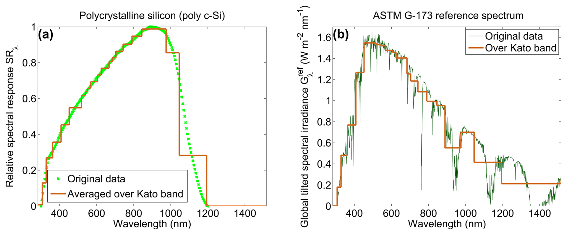
Figure 1 (a) Relative spectral response (on vertical axis) of polycrystalline silicon cell as function of wavelength (on horizontal axis). (b) ASTM G173-03 reference spectrum (on vertical axis) as function of wavelength (on horizontal axis). Original data in green and over Kato bands in orange. The spectral response is defined over the wavelength range from 300 to 1200 nm. Out of this wavelength range, the spectral response is 0.

Knowing that spectral resolution of KB is used for radiative transfer computations as described in Sect. 4.1, Eq. (1) may be computed by a Riemann sums over KBj mathematically defined as follows:

$$\begin{array}{}\text{(2)}& \text{SMF}={\displaystyle \frac{{\sum }_{j=\mathrm{1}}^{\mathrm{32}}{G}_{\mathrm{KB}j}^{\mathrm{T}}{\text{SR}}_{\mathrm{KB}j}}{{\sum }_{j=\mathrm{1}}^{\mathrm{32}}{G}_{\mathrm{KB}j}^{\mathrm{T}}}}{\displaystyle \frac{{\sum }_{j=\mathrm{1}}^{\mathrm{32}}{G}_{\mathrm{KB}j}^{\mathrm{ref}}}{{\sum }_{j=\mathrm{1}}^{\mathrm{32}}{G}_{\mathrm{KB}j}^{\mathrm{ref}}{\text{SR}}_{\mathrm{KB}j}}},\end{array}$$

where $G_{\mathrm{KB}j}^{\mathrm{T}}$ is the global irradiance on the tilted PV plane for KBj either under clear and cloudy sky situations, SR_KBj the averaged value of spectral response for KBj shown in orange line on Fig. 1a and $G_{\mathrm{KB}j}^{\mathrm{ref}}$ the global titled irradiance for KBj as illustrated in orange line in Fig. 1b.

Considering the relevance of spectral effects and limited studies in the literature, the behaviour of SMF still require further detailed investigations. This is especially the case of PV installations in clean and turbid atmospheres under overcast sky conditions, the sky conditions of interest to us. Such atmospheric conditions are representative of those existing at the four experimental PV sites being monitored.

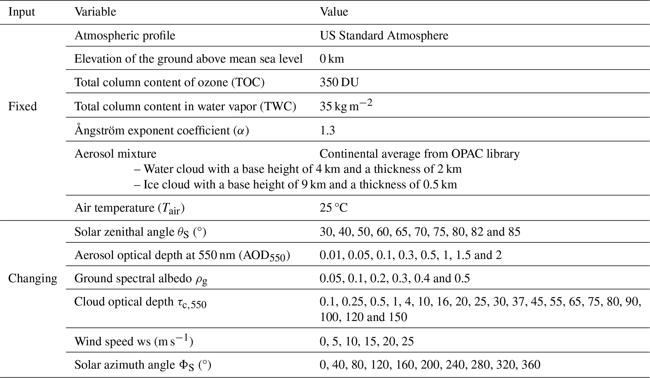
To perform the modelling assessment, atmospheric conditions and PV module geometric orientations should be defined. The following set of atmospheric conditions is selected: U.S. Standard Atmosphere, TOC of 350 DU, TWV of 35 kg m⁻², aerosol type of continental average from OPAC library of Hess et al. (1998), Ångström exponent coefficient of 1.3 and PV site elevation of 0 km as well as water (ice) cloud at medium (high) altitude with base height of 4 km (9 km) and a thickness of 2 km (0.5 km) respectively. These cloud geometrical properties are based on typical values for medium level water cloud and thin ice cloud (Liou, 1976; Rossow and Schiffer, 1999). This set is combined with ρ_g and AOD₅₅₀ values taken from Table 3; τ_c,550 values are selected from Table 4, both tables reported in Sect. 4.3 for the sake of simplicity; θ_S values in the set $\left\{\mathrm{40}\mathit{°};\mathrm{60}\mathit{°};\mathrm{80}\mathit{°}\right\}$ and the solar azimuth angle Φ_S = 100°. Each atmospheric state obtained from these combinations is an input to libRradtran. Each irradiance output per KB is then converted into irradiance onto titled place under various PV geometric orientations by using Eqs. (A1)–(A5) explicitly given in Appendix A. PV module geometric orientations are defined from the combinations between Φ_T = 180° and various θ_T values equal to 15°, 30°, 90°. The titled irradiances simulated are conveniently used following Eq. (2) for calculating SMF.

Table 3 Ranges and statistical distributions of values taken by the ground albedo, the elevation of the ground above mean sea level or PV site elevation and the six variables describing the clear-sky atmosphere.

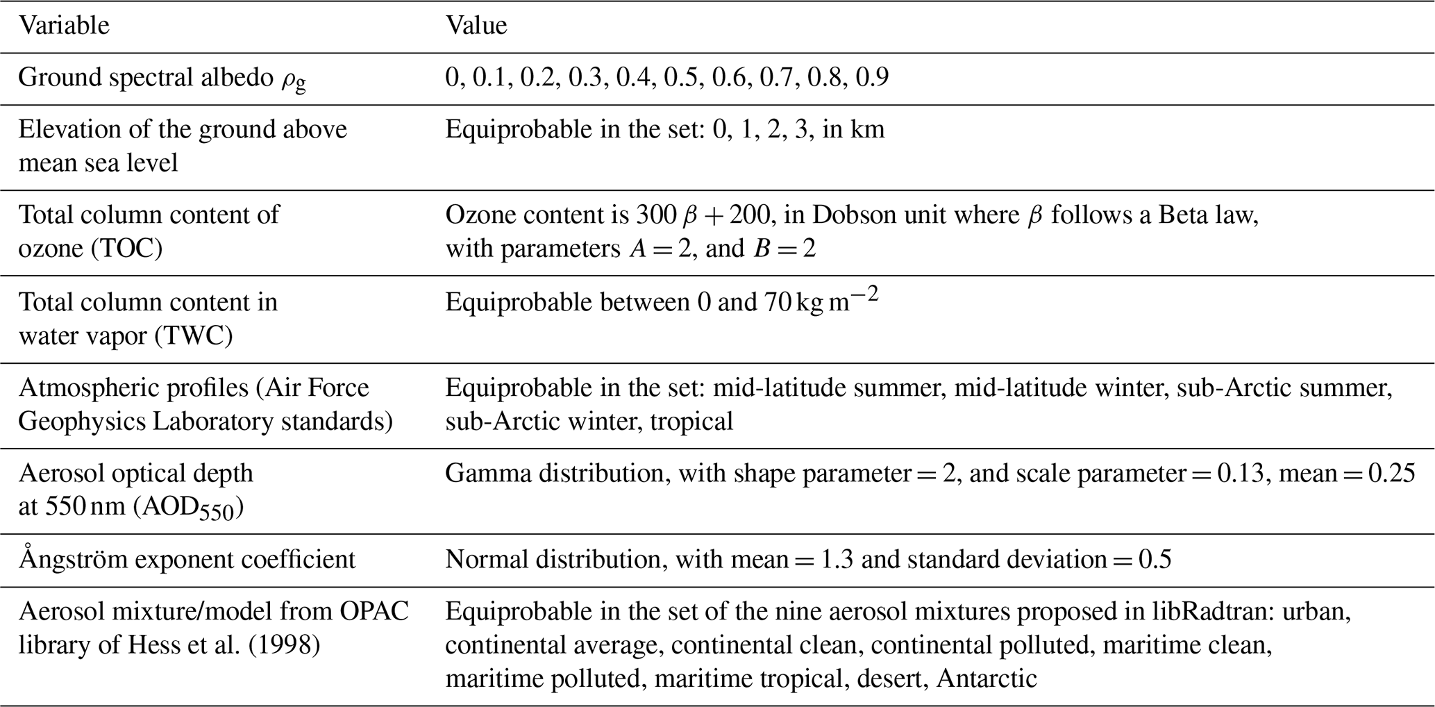
Table 4 Selected cloud properties. Mostly from Oumbe et al. (2014). Types of clouds and their acronyms; cumulus (Cu); stratocumulus (Sc); altostratus (As); altocumulus (Ac); cirrus (Ci); Stratus (St); Nimbostratus (Ns); Cumulonimbus (Cb) and cirrostratus (Cs).

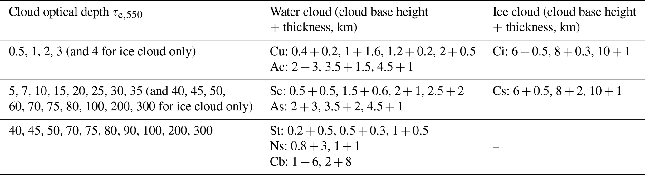
Figure 4 is an example of scatterplot between simulated SMF of polycrystalline silicon cell on vertical axis and ln (τ_c,550) on horizontal axis as a function of θ_S and θ_T for ρ_g = 0.2 and two contrasting aerosol loading conditions with water cloud: a clean atmosphere by AOD₅₅₀ = 0.01 (Fig. 2a) and a turbid atmosphere by AOD₅₅₀ = 1 (Fig. 2b). In general, SMF increases with increasing τ_c,550 whatever the atmospheric state and PV geometry. The graph linking SMF and ln (τ_c,550) has a characteristic of S-shaped or sigmoid curve. The analysis reveals that the shape of the curve and its magnitude is not sensitive to the ground albedo, i.e., the surface type.

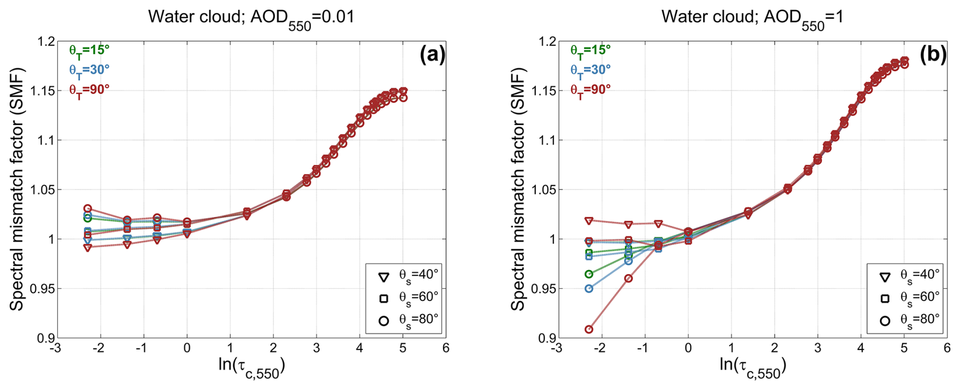
Figure 2 Scatterplot between SMF of polycrystalline silicon cell on vertical axis and ln (τ_c,550) on horizontal axis for various θ_S and θ_T and for two contrasting aerosol loading conditions with water cloud: a clean atmosphere by AOD₅₅₀ = 0.01 (Fig. 2a) and a turbid atmosphere by AOD₅₅₀ = 1 (Fig. 2b).

For ${\mathit{\tau }}_{\mathrm{c},\mathrm{550}}\ge$1, i.e., ln (τ_c,550) ≥ 0, the spread of dots is very limited and the coloured dots are almost superimposed exhibiting the weak dependence with the atmospheric state and PV module geometric orientations. SMF is greater than 1 with a maximum value of 1.18 implying a spectral gain reached up to 18 % experienced by the PV module. One may conclude, the thicker the cloud, the greater the spectral gain. Nevertheless, exceptions are seen for τ_c,550 < 1 representing optically thin clouds where the thinner the cloud, the larger the deviations of SMF. In a few turbid atmospheric conditions and associated PV module geometric orientations, SMF lie within 0.9 and 1 meaning a spectral loss of up to 10 %.

Similar findings were obtained when dealing with ice cloud (not shown). Further assessments were carried out when using other PV technologies. In sum, investigations clearly show significant impacts of SMF varying between wide gains or losses depending on actual atmospheric conditions and associated PV module geometric orientations. This imposes a necessity to fully account for SMF.

4.3 Sensitivity analysis on the relationship between $K_{\mathrm{c}}^{\mathrm{PV}}$ and τ_c

The main goal of the sensitivity analysis (SA) is to identify, among all inputs of the developed method, important (unimportant) variables/inputs, i.e., having significant (non-significant) impacts on τ_c estimates. SA, as an essential ingredient of $K_{\mathrm{c}}^{\mathrm{PV}}$–LUT building, consists of efficiently measuring the impact of an uncertain input on the relationship between $K_{\mathrm{c}}^{\mathrm{PV}}$ and τ_c. As a consequence, SA allows us to set a fixed value to each unimportant variable and thereby simplify our approach.

The present case study of flat roofs is defined with fixed tilt orientation and crystalline silicon PV systems at a given location. As introduced above, all-sky PV power computationally depends also on the atmospheric variables namely θ_S, Φ_S computed with the SG2 algorithm (Blanc and Wald, 2012). In addition, it also depends on atmospheric variables namely ρ_g, TOC, TWV, AOD and aerosol type, the vertical profiles of the temperature, pressure, density, and volume mixing ratio for gases, PV site elevation, ws, T_air as well as cloud properties namely CP, τ_c,550, effective radius of water droplets and ice crystals, cloud base height and thickness. While θ_T, Φ_T, θ_S and Φ_S are accurately known, the influence of remaining variables is examined on the nature of the relationship between $K_{\mathrm{c}}^{\mathrm{PV}}$ and τ_c.

For doing so, reference conditions close to the American Society for Testing and Materials (ASTM) G173 conditions are used here. ASTM conditions adopted by the PV community are made for performance comparisons of PV devices from different manufacturers and research laboratories under Standard Test Conditions (Kouklaki et al., 2023). The reference conditions are defined with θ_T = 37°, Φ_T = 180°, θ_S = 48.19°, Φ_S = 100°, U.S. Standard Atmosphere, TOC = 343.8 DU, TWV = 14.16 kg m⁻², aerosol urban type from OPAC library of Hess et al. (1998) with an AOD₅₅₀ = 0.074 and Ångström exponent coefficient of 1.3, an ideal ground with a spectrally constant ρ_g = 0.2 and are associated with cloud properties (as explained in Sect. 4.1) yielding to produce a set of various realistic conditions. A SA is carried out by means of the combination of libRadtran and PV model. It is performed by changing one of the analyzed variables at a time.

Table 3 reports the range of values taken respectively by ρ_g and the seven other variables describing the clear-sky atmosphere. These variables are randomly generated following the modelled marginal distribution established from observations proposed by Lefèvre et al. (2013) and used by e.g., Wandji Nyamsi et al. (2015b, 2017, 2019, 2020, 2021), Thomas et al., 2023). Specifically, the uniform distribution was chosen as a model for the marginal probability of all parameters except AOD₅₅₀ and TOC for which the chi-square and beta laws were selected respectively.

Each ρ_g value was associated with each of the 1000 random selections of the other seven variables in Table 3 providing a set of 10 000 clear-sky atmospheric states. Then, each clear-sky atmospheric state was associated with one combination of τ_c,550, cloud base height, thickness and cloud phase as reported in Table 4. Values are related to types of clouds to produce realistic conditions. This yielded 1 540 000 (10 000 clear-sky atmospheric states times 154 combinations of cloudy properties) atmospheric conditions for water clouds and 690 000 (10 000 clear-sky atmospheric states times 69 combinations of cloudy properties) atmospheric conditions for ice clouds.

To complete the setup of inputs associated to previous atmospheric states and needed specifically for PV model, T_air is set to follow the uniform distribution between −35 and 50 °C while ws (m s⁻¹) is chosen randomly in the set $\left\{\mathrm{0},\mathrm{5},\mathrm{10},\mathrm{15},\mathrm{20},\mathrm{25}\right\}$. In practice and under both clear and cloudy sky situations, for a given PV site with specific geometric orientation and atmospheric state, the PV model is literally applied from Eqs. (A1)–(A9) explicitly given in Appendix A for each KBj. SMF is computed from Eq. (2). Then, the total effective irradiance of PV panel, denoted $G_{\mathrm{eff}}^{\mathrm{T}}$ over the shortwave solar spectrum of Eq. (A10) is replaced with $G_{\mathrm{eff}}^{\mathrm{T}}$ = SMF ${\sum }_{j=\mathrm{1}}^{\mathrm{32}}{G}_{{\mathrm{eff}}_{\mathrm{KB}}j}^{\mathrm{T}}$. Then, the remaining equations of the PV model are used as is. This yields to PV power estimates under both clear and cloudy sky situations thus allowing to compute $K_{\mathrm{c}}^{\mathrm{PV}}$.

Figure 3 displays an example of a scatterplot between $K_{\mathrm{c}}^{\mathrm{PV}}$ on horizontal axis and ln (τ_c,550) on vertical axis for water (Fig. 3a) and ice (Fig. 3b) clouds separately with all TOC, TWV, aerosol type, atmospheric profiles, PV site elevation, T_air, cloud base height and thickness varying but AOD₅₅₀ = 0.074, ρ_g = 0.2 and ws = 5 m s⁻¹ kept fixed. In general, the curve of the relationship between $K_{\mathrm{c}}^{\mathrm{PV}}$ and ln (τ_c,550) shows the form of an exponential decay function or $K_{\mathrm{c}}^{\mathrm{PV}}$ have a strong inversely proportional relation with ln (τ_c,550) for both cloud phases. τ_c,550 increases with decreasing $K_{\mathrm{c}}^{\mathrm{PV}}$ indicating, as expected, that the thicker the cloud, the stronger the cloud attenuation on solar radiation and then the lower the PV power. The spread of dots is very limited and are almost superimposed meaning that the individual/collective uncertainty of these analysed variables has negligible impact on τ_c estimates. Consequently, this result makes them unimportant variables.

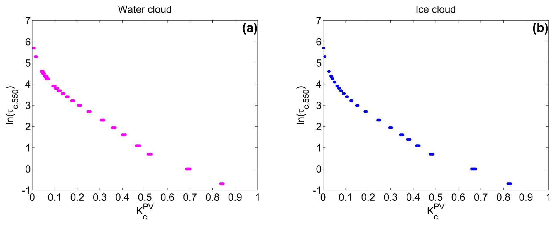
Figure 3 Scatterplot between $K_{\mathrm{c}}^{\mathrm{PV}}$ on horizontal axis and ln (τ_c,550) on vertical axis by varying all parameters except AOD₅₅₀ = 0.074, ρ_g = 0.2 and ws = 5 m s⁻¹. (a) For water cloud and (b) for ice cloud.

Figure 4 shows ln (τ_c,550) on vertical axis plotted versus $K_{\mathrm{c}}^{\mathrm{PV}}$ on horizontal axis, left side for water cloud and right side for ice cloud, as function of AOD₅₅₀. Other variables have been kept fixed with previously mentioned values. The form of the curves is like those in Fig. 3. The spread of colored dots for each class of AOD is noticeable although it decreases towards thicker clouds. This means the AOD has a strong impact on τ_c estimates making AOD an important variable. Similar findings (not shown) were observed when applying the SA on ρ_g and ws making these latter to be important too.

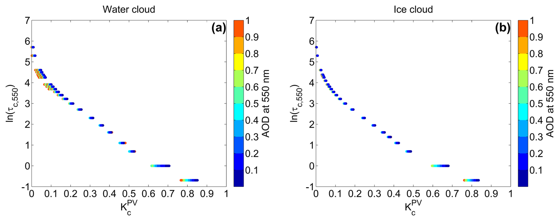
Figure 4 Scatterplot between $K_{\mathrm{c}}^{\mathrm{PV}}$ on horizontal axis and ln (τ_c,550) on vertical axis for various classes of AOD at 550 nm. (a) For water cloud and (b) for ice cloud. The color-bar indicates the AOD range.

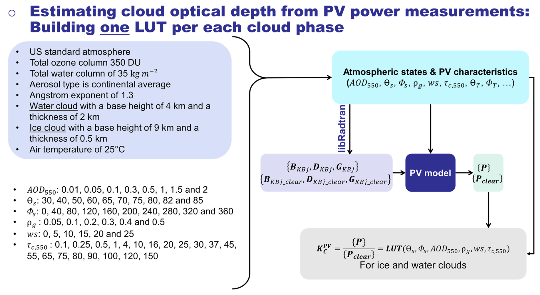
In summary, for a given geometrical PV geometric orientation, variables θ_S, Φ_S, AOD, ρ_g, ws and $K_{\mathrm{c}}^{\mathrm{PV}}$ are important to consider when estimating τ_c. A practical advantage of such analysis is that $K_{\mathrm{c}}^{\mathrm{PV}}$–LUT can be computed with typical values of other variables kept constant, therefore strongly reducing the size of the LUT and thus increasing the speed in computation. One may select the following set as selected in Sect. 4.2 namely U.S. Standard Atmosphere, TOC of 350 DU, TWV of 35 kg m⁻², aerosol type of continental average, Ångström exponent coefficient of 1.3 and PV site elevation of 0 km as well as water (ice) cloud at medium (high) altitude with base height of 4 km (9 km) and a thickness of 2 km (0.5 km) respectively. This typical set of atmospheric conditions is used in the rest of this paper.

4.4 Building $K_{\mathrm{c}}^{\mathrm{PV}}$–LUT and estimating effective cloud optical depth (${\mathit{\tau }}_{\mathrm{c}}^{\mathrm{eff}}$)

Two LUTs were constructed for a limited number of node points, one for each cloud phase. Table 5 summarizes the number of node points selected for building $K_{\mathrm{c}}^{\mathrm{PV}}$–LUT as follows: $K_{\mathrm{c}}^{\mathrm{PV}}$ = $f({\mathit{\theta }}_{\mathrm{S}},{\mathit{\rho }}_{\mathrm{g}},{\text{AOD}}_{\mathrm{550}},{\mathrm{\Phi }}_{\mathrm{S}},\text{ws},{\mathit{\tau }}_{\mathrm{c},\mathrm{550}})$. For a given PV site with specific geometric orientation, both libRadtran and PV model are used as earlier in order to compute for each combination obtained following node points. For the sake of reproducibility and practicality, the procedure on how to build the ${\mathrm{K}}_{\mathrm{c}}^{\mathrm{PV}}$–LUT is summarized and exhibited in Fig. 5.

Table 5 Ranges of values taken by each input for building $K_{\mathrm{c}}^{\mathrm{PV}}$–LUT.

Figure 5 Schematic structure showing how to build the $K_{\mathrm{c}}^{\mathrm{PV}}$–LUT.

The goal of this study is to estimate ${\mathit{\tau }}_{\mathrm{c}}^{\mathrm{eff}}$. In order to derive ${\mathit{\tau }}_{\mathrm{c}}^{\mathrm{eff}}$, $K_{\mathrm{c}}^{\mathrm{PV}}$ values are simulated from $K_{\mathrm{c}}^{\mathrm{PV}}$–LUT and these simulated values are compared with the corresponding measured one. The τ_c,550 input values vary from 0.1 to 150. The value of τ_c,550 that minimises the difference between the measured and simulated $K_{\mathrm{c}}^{\mathrm{PV}}$ is considered as the estimated ${\mathit{\tau }}_{\mathrm{c}}^{\mathrm{eff}}$ from PV power measurements. The term “effective” or superscript eff indicates the τ_c,550 value that is used as input into the $K_{\mathrm{c}}^{\mathrm{PV}}$–LUT and that best matches with experimental PV power data.

4.5 Practical implementation of the proposed method

Figure 6 summarizes how to implement the developed method for estimating ${\mathit{\tau }}_{\mathrm{c}}^{\mathrm{eff}}$ from PV power measurements in a tractable manner for a given PV system when combining various sources of inputs. Prior to the execution of the proposed method, the $K_{\mathrm{c}}^{\mathrm{PV}}$–LUT for a PV site is built based on PV characteristics namely geocoordinates, orientation, nominal capacity and so on for both ice and water clouds. Aerosol properties, sun position angles, ground albedo as well as downwelling shortwave irradiance and its direct and diffuse components received at ground level under clear-sky conditions at 1 min temporal resolution are obtained by machine-to-machine calls to the Web service CAMS on the SoDa Service. With PV power measurements and PV model, CAMS data and wind speed and air temperature at every 1 min obtained by linear interpolation functions from 1-hourly ECMWF ERA5 data are used to produce calibrated clear-sky time series of PV power. Both measured and calibrated clear-sky PV power combined with satellite information are then used to detect overcast sky conditions with corresponding cloud phase either water or ice clouds. Only under overcast sky conditions and for the corresponding cloud phase, 1 min CAMS atmospheric variables and wind speed combined with τ_c,550 values varying between 0.1 and 150 are as inputs to $K_{\mathrm{c}}^{\mathrm{PV}}$–LUT. A series of interpolation functions are performed to yield the estimated $K_{\mathrm{c}}^{\mathrm{PV}}$ for a given τ_c value. This later process continues in the trial-and-error process until the minimum difference between $K_{\mathrm{c}\mathrm{\_}\mathrm{meas}}^{\mathrm{PV}}$ and estimated $K_{\mathrm{c}}^{\mathrm{PV}}$ is reached. The varied τ_c value providing such minimum is the effective τ_c value.

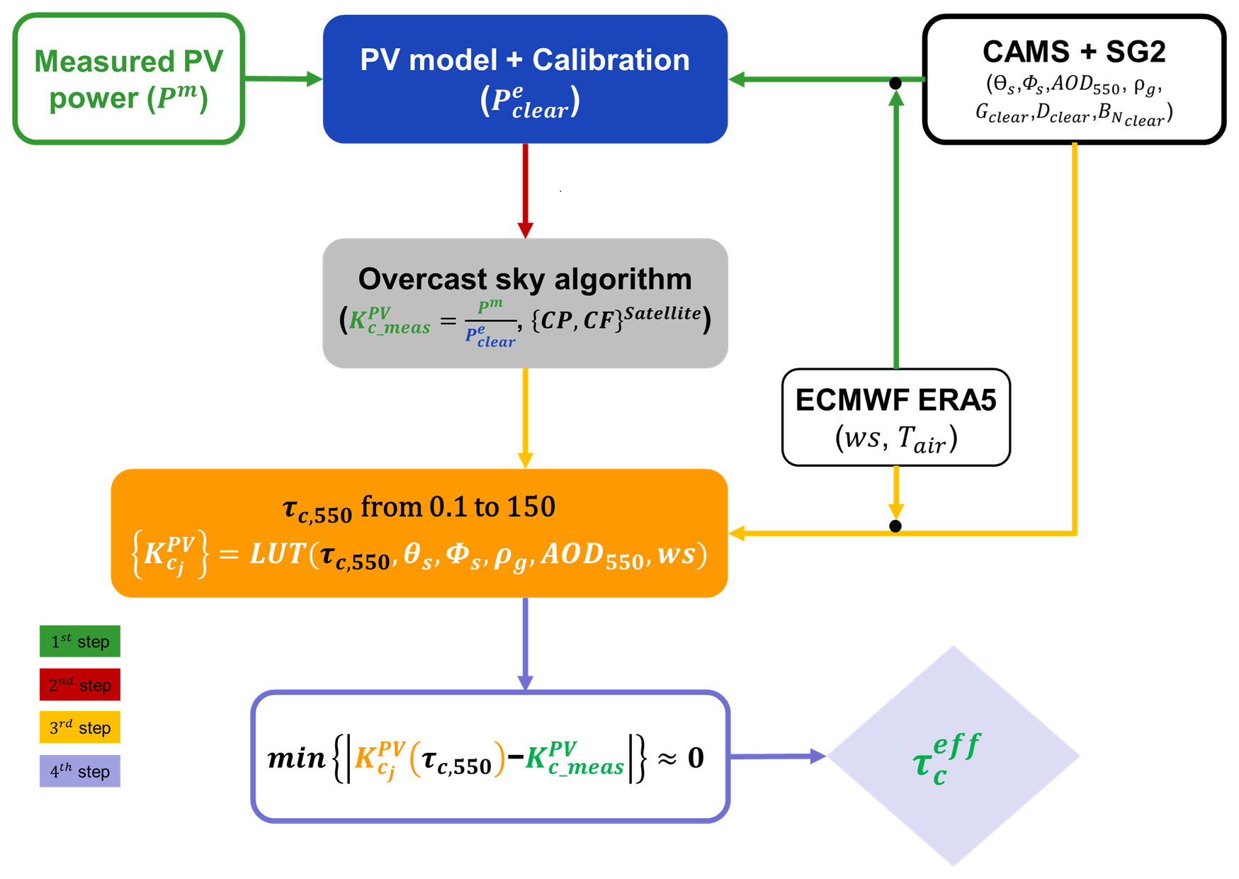
Figure 6 Sketch of developed method for estimating cloud optical depth from PV power measurements.

5 Results and discussion

Estimated ${\mathit{\tau }}_{\mathrm{c}}^{\mathrm{eff}}$ from the proposed method were compared individually to the τ_c retrievals from (1) ground-based G measurements denoted ${\mathit{\tau }}_{\mathrm{c}}^G$ using the empirical equation by Barnard and Long (2004) and (2) ${\mathit{\tau }}_{\mathrm{c}}^{\mathrm{MODIS}}$ and (3) ${\mathit{\tau }}_{\mathrm{c}}^{\mathrm{CAMS}}$ each one serving as reference. For comparisons with satellite retrievals, 15 min averaged ground-based ${\mathit{\tau }}_{\mathrm{c}}^{\mathrm{eff}}$ centered on the satellite observation time have been compared to instantaneous observation satellite ${\mathit{\tau }}_{\mathrm{c}}^{\mathrm{MODIS}}$ or ${\mathit{\tau }}_{\mathrm{c}}^{\mathrm{CAMS}}$. Similar procedure in averaging times has been used in numerous previous studies (Dong et al., 2008; Xi et al., 2014; Yan et al., 2015; Sporre et al., 2016; Li et al., 2019; Aebi et al., 2020). With MODIS data, only satellite observation pixels having their centers at a maximum distance of 10 km away from the PV site are retained for analysis. The averaged value computed from those retained pixel values is assumed to represent the instantaneous observation satellite ${\mathit{\tau }}_{\mathrm{c}}^{\mathrm{MODIS}}$. This would still validate the hypothesis that time and space averages are interchangeable (Chiu et al., 2010). Relevant cloud phase either water or ice cloud is obtained by the means of CP^CAMS or CP^MODIS depending on the satellite used. This CP allows to select the correct $K_{\mathrm{c}}^{\mathrm{PV}}$–LUT either for water cloud or for ice cloud. When overcast sky periods are selected with either CAMS or MODIS data, 15 min averaged ground-based ${\mathit{\tau }}_{\mathrm{c}}^{\mathrm{eff}}$ are compared to 15 min averaged ground-based ${\mathit{\tau }}_{\mathrm{c}}^G$.

Following the ISO standard (International Organization for Standardization, 1995), the deviations or errors, i.e., estimate minus reference were calculated. They were synthesized with the Bias (mean error), the root mean square error (RMSE), and their values rBias and rRMSE relative to the mean value of the reference values. In addition, the coefficient of correlation (R) is calculated. It is well known that satellite- and ground-based retrievals at very large θ_S are often subjected of high uncertainties. Consequently, all comparisons are performed only for θ_S ≤ 80 ° to avoid overly small signals (Barker et al., 1998). In addition, to avoid potential effects from snow contamination on any τ_c retrievals due to snow deposit on PV modules, the comparisons are performed only from June to September of each year.

5.1 Comparison of estimated ${\mathit{\tau }}_{\mathrm{c}}^{\mathrm{eff}}$ with ${\mathit{\tau }}_{\mathrm{c}}^G$

Instantaneous ${\mathit{\tau }}_{\mathrm{c}}^G$ are derived from the empirical equation by Barnard and Long (2004) mathematically defined as follows:

$$\begin{array}{}\text{(3)}& {\mathit{\tau }}_{\mathrm{c}}^G=e^{\left[\mathrm{2.15}+{\mathit{\rho }}_{\mathrm{g}}^{\mathrm{CAMS}}+\mathrm{1.91}\text{arctanh}\left(\mathrm{1}-\mathrm{1.74}\frac{G^{\mathrm{m}}}{G_{\mathrm{clear}}^{\mathrm{CAMS}}{\left(\cos \left({\mathit{\theta }}_{\mathrm{S}}\right)\right)}^{\frac{\mathrm{1}}{\mathrm{4}}}}\right)\right]},\end{array}$$

where G^m is the measured G and the superscript CAMS referring to values obtained from CAMS data.

Figure 7 exhibits, for each station, the scatter density plot of 15 min averages between ${\mathit{\tau }}_{\mathrm{c}}^G$ retrievals (horizontal axis) and ${\mathit{\tau }}_{\mathrm{c}}^{\mathrm{eff}}$ estimates (vertical axis) from the proposed method for water clouds under overcast sky conditions when using CF^CAMS. The station name and the temporal period are indicated at the top of each plot. In general, all points are well located along the identity line with a limited scattering.

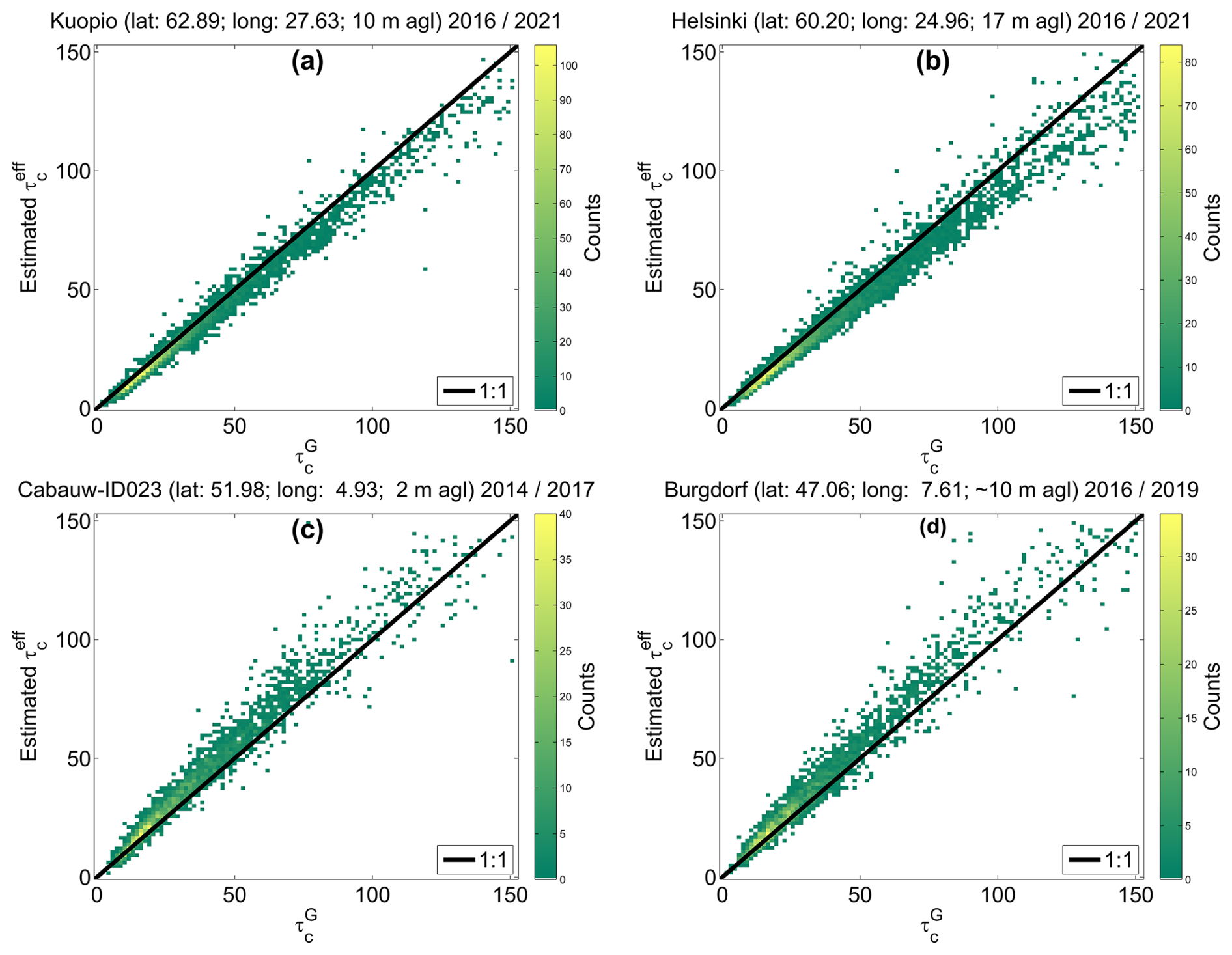
Figure 7 2D histograms of 15 min averages between ${\mathit{\tau }}_{\mathrm{c}}^G$ retrievals (horizontal axis) and ${\mathit{\tau }}_{\mathrm{c}}^{\mathrm{eff}}$ estimates (vertical axis) for water clouds at (a) Kuopio, (b) Helsinki, (c) Cabauw–ID023 and (d) Burgdorf when using CF^CAMS for selecting overcast sky conditions. The color indicates the number of pairs in the area within the interval 1.5 × 1.5.

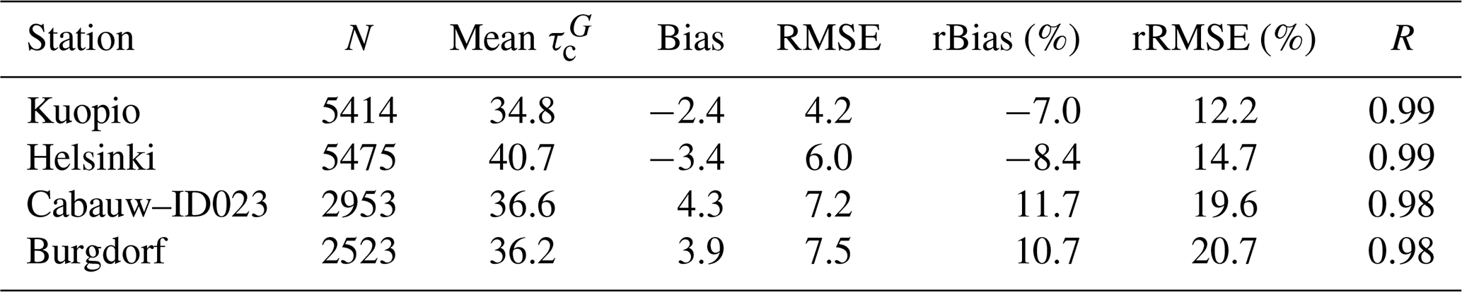
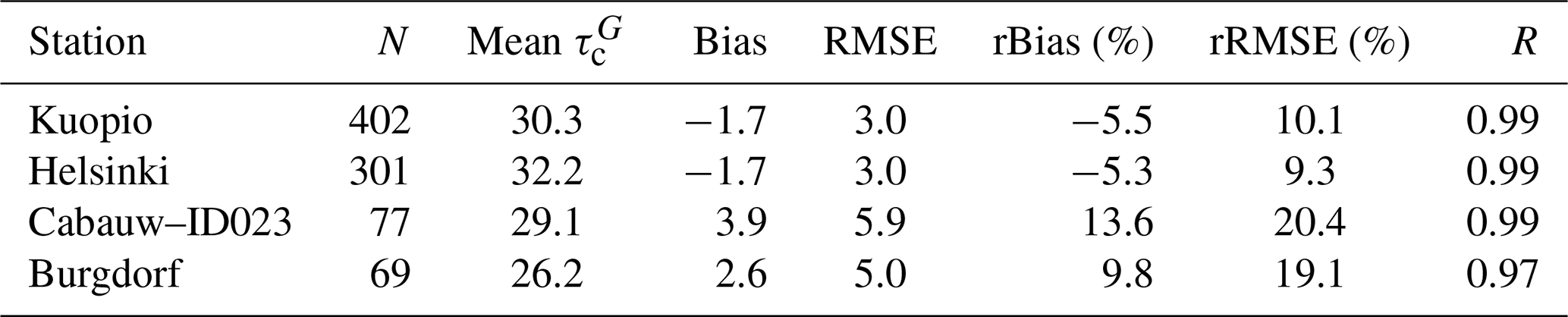
Statistical indicators summarizing the errors in τ_c retrievals for each station and for water clouds are reported in Table 6. The correlation coefficient R is very high and greater than 0.98 in all stations denoting that the variability in ${\mathit{\tau }}_{\mathrm{c}}^G$ is very well explained by the ${\mathit{\tau }}_{\mathrm{c}}^{\mathrm{eff}}$ estimates. The bias is low ranging between –3 and 4, i.e., −8 % (Helsinki) and 12 % (Cabauw–ID023) in relative value with respect to the mean value of ${\mathit{\tau }}_{\mathrm{c}}^G$. This shows a high level of agreement of ${\mathit{\tau }}_{\mathrm{c}}^{\mathrm{eff}}$. The RMSE is small lying in the interval [4, 8] ([12, 21] % in relative value with respect to the mean value of ${\mathit{\tau }}_{\mathrm{c}}^G)$. One observes that the largest spreads of points are seen in Cabauw–ID023 and Burgdorf. The errors observed in the comparison may be caused by a number of factors including three-dimensional radiative effects, assumptions on the state of the atmosphere such as aerosol load, details related to modelling of the PV power output, and measurement uncertainties. In general, the proposed method shows very good performance, and a very good level of accuracy is reached that is close to the uncertainty of the reference value themselves.

Table 6 Statistical indicators of the performance of the novel method for retrieving τ_c for water clouds when using CAMS data. N is the number of samples.

Similarly to Fig. 7, results for each station of 15 min average comparisons between ${\mathit{\tau }}_{\mathrm{c}}^G$ retrievals (horizontal axis) and ${\mathit{\tau }}_{\mathrm{c}}^{\mathrm{eff}}$ estimates (vertical axis) from the proposed method for water clouds under overcast sky conditions when using CF^MODIS are shown in Fig. 8.

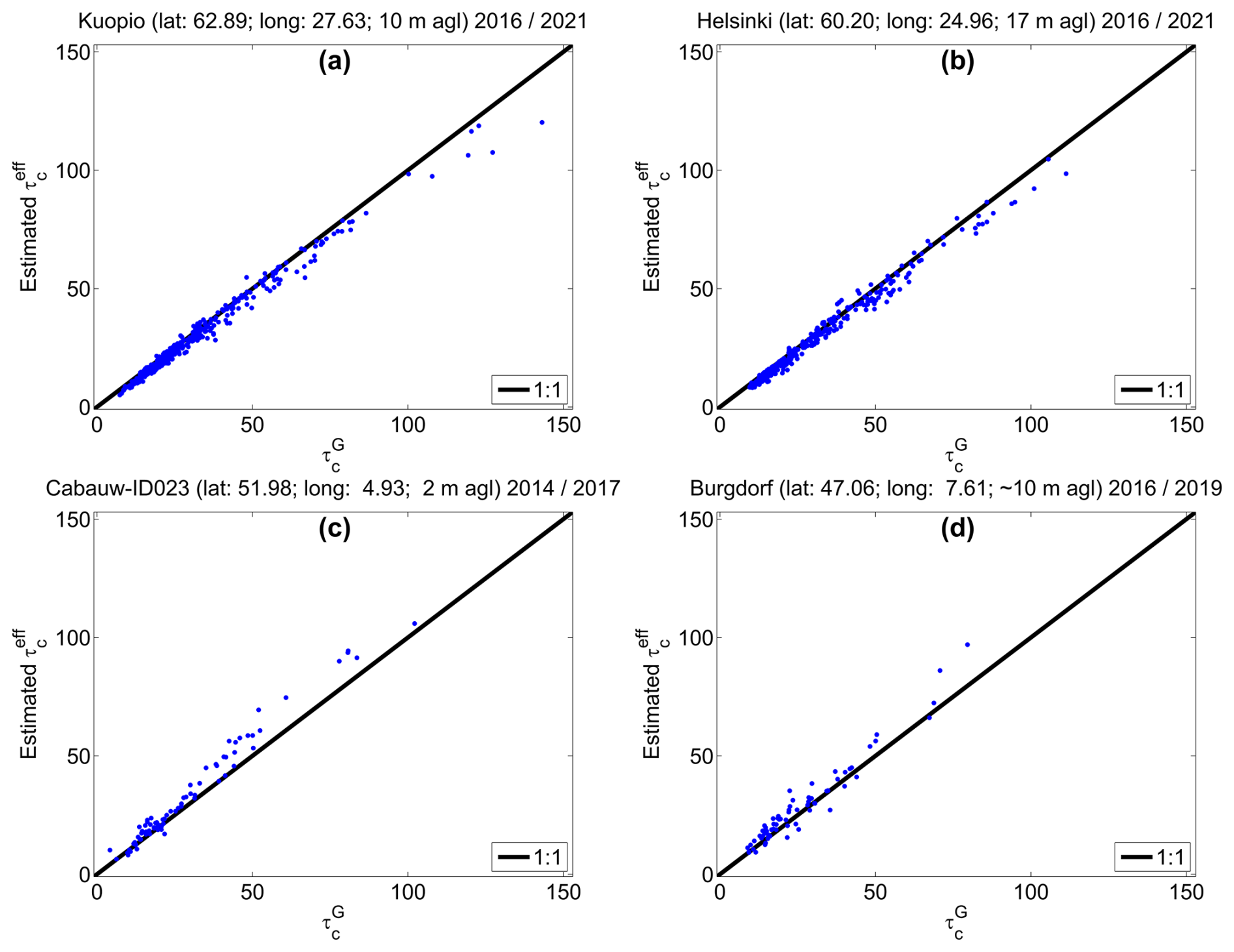
Figure 8 Scatterplots of 15 min averages between ${\mathit{\tau }}_{\mathrm{c}}^G$ retrievals (horizontal axis) and ${\mathit{\tau }}_{\mathrm{c}}^{\mathrm{eff}}$ estimates (vertical axis) for water clouds at (a) Kuopio, (b) Helsinki, (c) Cabauw–ID023 and (d) Burgdorf when using CF^MODIS for selecting overcast sky conditions.

Although the number of samples are much smaller than compared to cases when using CF^CAMS (Fig. 7 and Table 6) due to the temporal coverage of MODIS data depending on satellite overpass times, the points in the graph are well elongated along the identity line with a limited spread of points (Fig. 8). At all stations, the correlation coefficient is mostly greater than 0.99 (Table 7) meaning that the ${\mathit{\tau }}_{\mathrm{c}}^{\mathrm{eff}}$ estimates reproduce well the variability in the ${\mathit{\tau }}_{\mathrm{c}}^G$ retrievals. The bias is small lying in the interval $[-\mathrm{2},\mathrm{4}]$ ($[-\mathrm{6},\mathrm{14}]$ % in values relative to the means of ${\mathit{\tau }}_{\mathrm{c}}^G$ retrievals at each station). The RMSE (rRMSE) is very limited, varying from 3 (9 %) to 6 (20 %). The level of performance in terms of the absolute value of errors could be explained for similar reasons as mentioned earlier. No comparisons here were made with ice clouds because the formula presented in the Eq. (3) is only designed for water clouds.

Table 7 Statistical indicators of the performance of the novel method for retrieving τ_c for water clouds when using MODIS data. N is the number of samples.

In general, the comparisons reveal that somewhat lower performance of the method is observed at Cabauw–ID023, compared to the three other sites. Only for this site with power measurements of rooftop mounted residential PV system and unfortunately, historic metadata information is not available due to privacy concerns (Visser et al., 2022). Such information is certainly considered to be the most efficient way to track down issues that might occur like inverter malfunctions, electrical issues and so on. When unavailable as is the case for Cabauw–ID023, it remains quite challenging to carry out further investigations to understand discrepancies. This emphasizes the need to obtain as much a priori metadata about the PV systems as possible when performing such τ_c retrievals.

5.2 Comparison of estimated ${\mathit{\tau }}_{\mathrm{c}}^{\mathrm{eff}}$ with ${\mathit{\tau }}_{\mathrm{c}}^{\mathrm{MODIS}}$

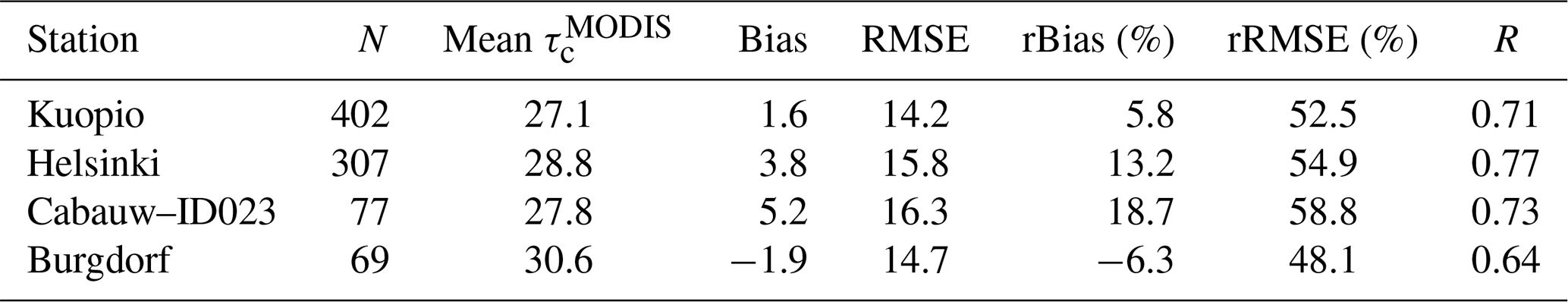
Fifteen-minute averages of ${\mathit{\tau }}_{\mathrm{c}}^{\mathrm{eff}}$ estimates are also compared with instantaneous ${\mathit{\tau }}_{\mathrm{c}}^{\mathrm{MODIS}}$ retrievals for water clouds and are shown in Fig. 9 for each station when using CF^MODIS. The amount of data is also limited here for similar reasons as reported earlier. In general, the cloud of the points follows the 1 : 1 line fairly well, with many points lying above this line. The correlation coefficient is greater than 0.70 except at Burgdorf (Table 8) having less than 70 data. This means that 49 % of the variance, i.e., the information contained in MODIS is explained by ${\mathit{\tau }}_{\mathrm{c}}^{\mathrm{eff}}$ estimates. In most cases, these latter show a tendency to slightly overestimate with a bias ranging between −2 (−6 %) and 5 (19 %). The RMSE (rRMSE) is large, varying between 14 (48 %) and 16 (59 %). The performance level of the proposed method at Cabauw–ID023 is at the lowest of all sites in terms of relative errors. Nevertheless, the results are consistent with similar studies carried out for stations in China and Switzerland (Li et al., 2019; Aebi et al., 2020). Overall, the proposed method exhibits a good level of accuracy.

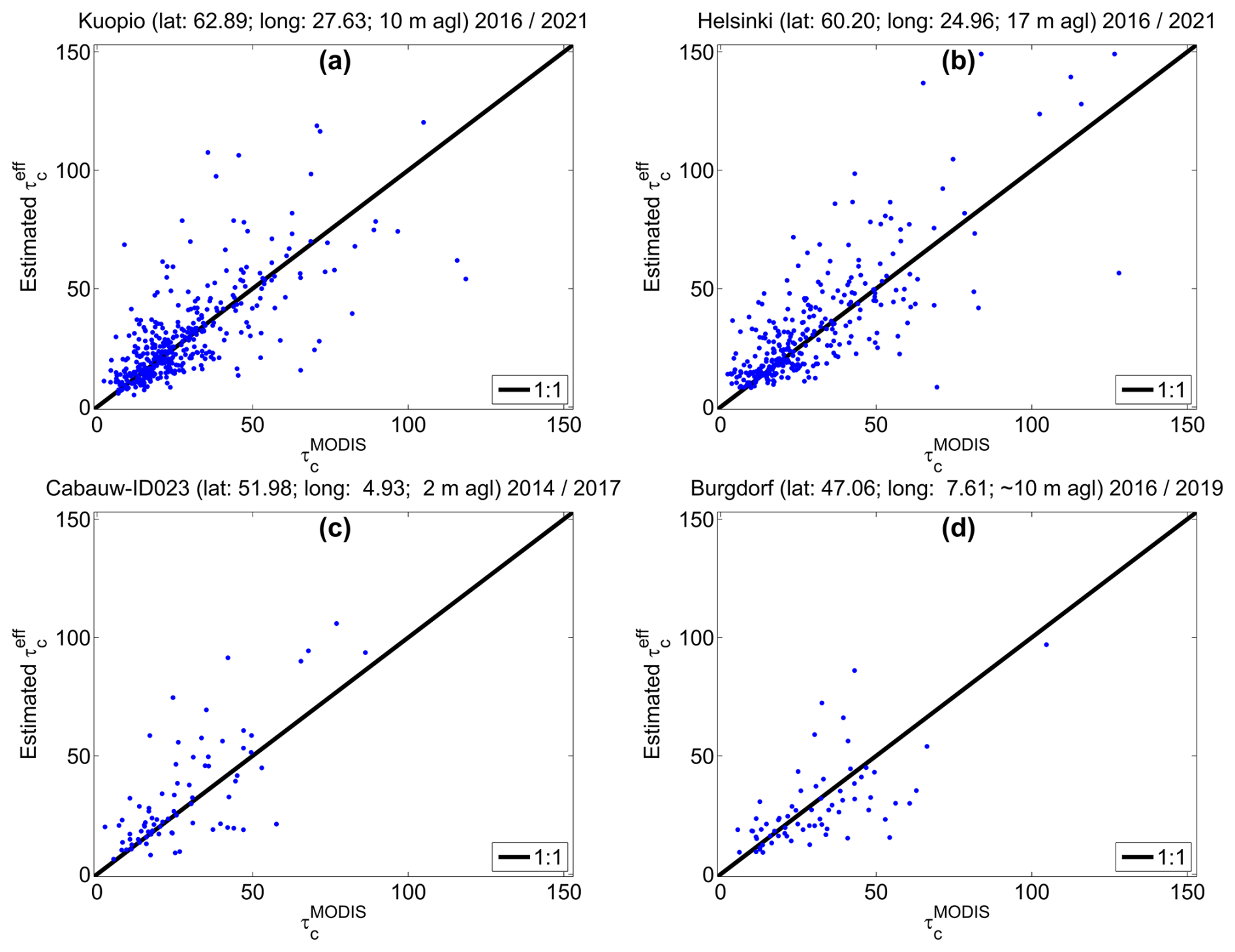
Figure 9 Scatterplots between instantaneous ${\mathit{\tau }}_{\mathrm{c}}^{\mathrm{MODIS}}$ retrievals (horizontal axis) and 15 min averages of ${\mathit{\tau }}_{\mathrm{c}}^{\mathrm{eff}}$ estimates (vertical axis) for water clouds at (a) Kuopio, (b) Helsinki, (c) Cabauw–ID023 and (d) Burgdorf when using CF^MODIS for selecting overcast sky conditions.

Table 8 Statistical indicators of the performance of the novel method for retrieving τ_c for water clouds when using MODIS data. N is the number of samples.

Results for ice clouds are shown in Fig. 10. In general, one observes that the cloud of the points follows the 1 : 1 line fairly well for τ_c lower than 50 with a very limited spread of points while for τ_c greater than 50 (for optically thick clouds), the spread of points is more pronounced. Knowing that uncertainties often increase with increasing τ_c specially for optically thick ice clouds, statistics are computed for two cases: τ_c ≤ 150 and τ_c ≤ 50. Corresponding statistical results are reported in Table 9.

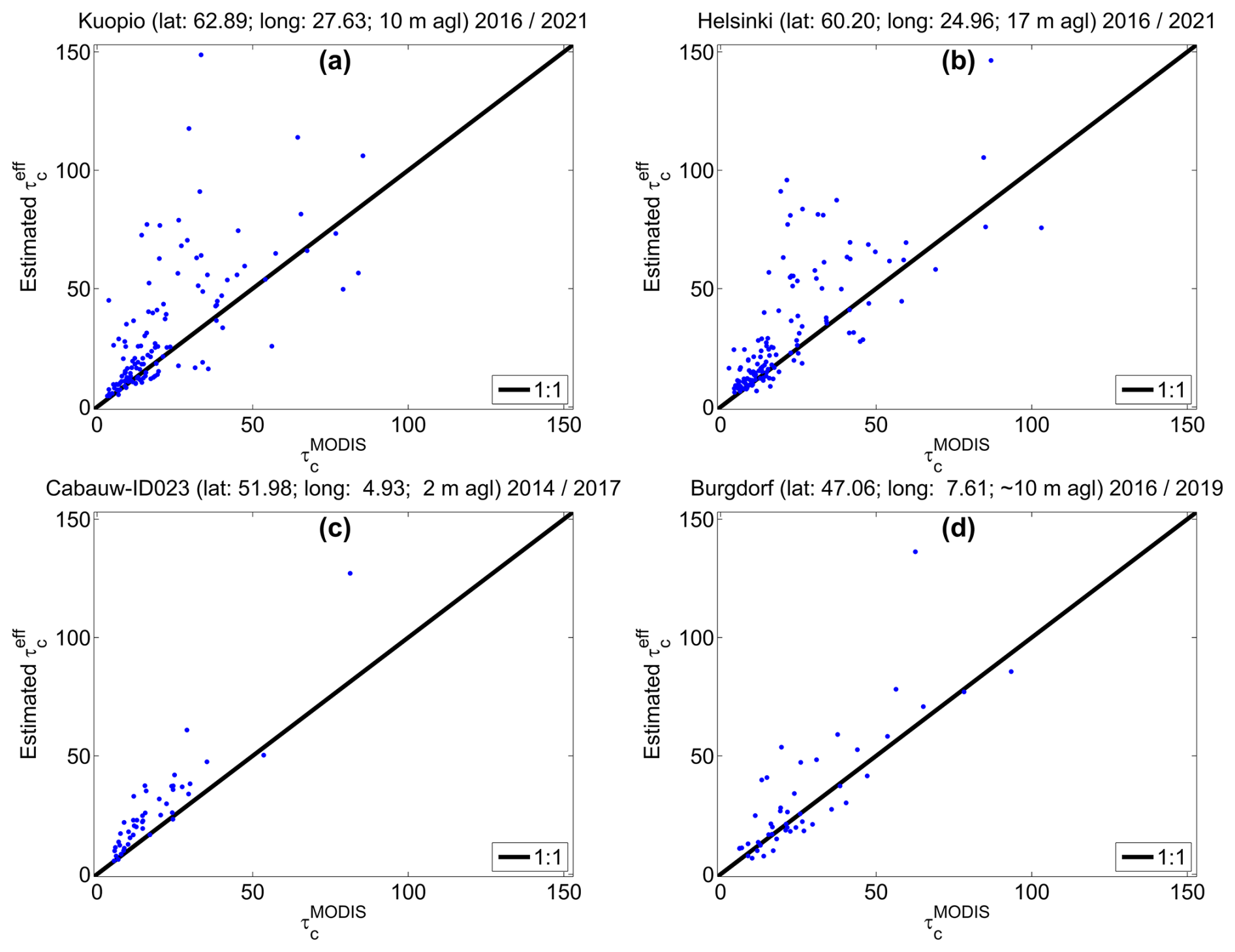
Figure 10 Scatterplots between instantaneous ${\mathit{\tau }}_{\mathrm{c}}^{\mathrm{MODIS}}$ retrievals (horizontal axis) and 15 min averages of ${\mathit{\tau }}_{\mathrm{c}}^{\mathrm{eff}}$ estimates (vertical axis) for ice clouds at b Kuopio, (b) Helsinki, (c) Cabauw–ID023 and (d) Burgdorf when using CF^MODIS for selecting overcast sky conditions.

Table 9 Statistical indicators of the performance of the novel method for retrieving τ_c for ice clouds when using MODIS data. N is the number of samples. The first value is for τ_c ≤ 150 and the second value is the τ_c ≤ 50 with the best performance in bold.

The correlation coefficient is mostly greater than 0.7 for both τ_c ranges. This implies that, to a certain degree, the ${\mathit{\tau }}_{\mathrm{c}}^{\mathrm{eff}}$ could be useful to observe and analyze the optical properties of ice clouds. The majority of the points lie above the 1 : 1 line denoting an overall overestimation of τ_c by the proposed method. The bias ranges between 2 (11 %) and 10 (51 %). The RMSE lies within [8;22], i.e., [46;105] %.

From the above statistics, one may observe ${\mathit{\tau }}_{\mathrm{c}}^{\mathrm{eff}}$ retrievals exhibit a better agreement when τ_c≤50 in all stations in terms of relative errors. Similar results were obtained at the best performance when comparing individually several satellite cloud products against those from MODIS (Lai et al., 2019; Liu et al., 2025). The accuracy level of the proposed method is best met at Burgdorf clearly showing great capabilities of the proposed method for providing routinely good τ_c retrievals. Although the overall performance level is satisfactory, some precautions should be considered when examining the results. For instance, because of the often unknown vertical and internal structure, the complex geometrical shapes and sizes of ice crystals and different microphysical assumptions, the inversion of ice clouds remains very challenging despite significant efforts to perfect retrieval algorithms and can lead to large uncertainties in τ_c retrievals (Li et al., 2019).

5.3 Comparison of estimated ${\mathit{\tau }}_{\mathrm{c}}^{\mathrm{eff}}$ with ${\mathit{\tau }}_{\mathrm{c}}^{\mathrm{CAMS}}$

Results of comparisons between instantaneous ${\mathit{\tau }}_{\mathrm{c}}^{\mathrm{CAMS}}$ (horizontal axis) and 15 min average estimates of ${\mathit{\tau }}_{\mathrm{c}}^{\mathrm{eff}}$ (vertical axis) are shown in Fig. 11 for each station for water clouds under overcast sky conditions selected by using CF^CAMS.

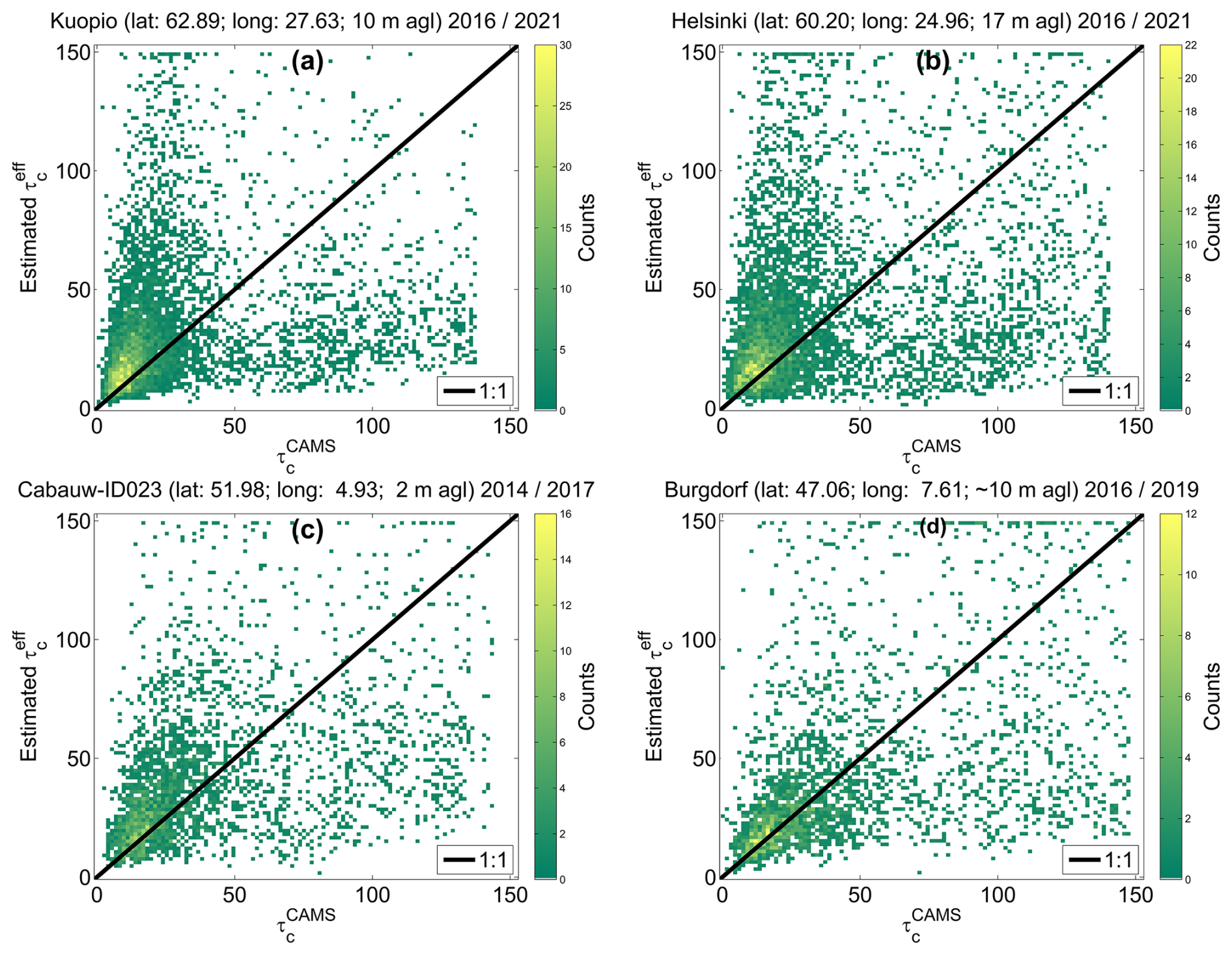
Figure 11 2D histograms of between instantaneous ${\mathit{\tau }}_{\mathrm{c}}^{\mathrm{CAMS}}$ retrievals (horizontal axis) and 15 min averages of ${\mathit{\tau }}_{\mathrm{c}}^{\mathrm{eff}}$ estimates (vertical axis) for water clouds at (a) Kuopio, (b) Helsinki, (c) Cabauw–ID023 and (d) Burgdorf when using CF^CAMS for selecting overcast sky conditions. The color indicates the number of pairs in the area within the interval 1.5 × 1.5.

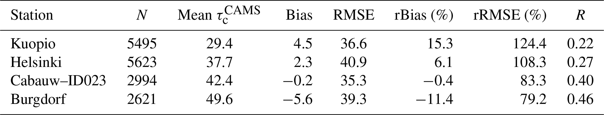
The spread of points is noticeable with a perceptible density of points for low τ_c values. Table 10 gives statistical quantities on the errors between both τ_c retrievals accordingly. In general, statistical indicators exhibit an overall latitudinal trend which tends to improve southwards. The correlation coefficient is low and ranges between 0.22 (Kuopio) and 0.46 (Burgdorf). The bias (rBias) is low and ranges between −6 (−11 %) in Burgdorf and 5 (15 %) in Kuopio. As expected from visual inspection of graphs, RMSE (rRMSE) is noticeable and ranges between 35 (79 %) and 41 (124 %). In terms of standard deviations, the largest (smallest) spread of points are seen in Kuopio (Burgdorf), the northernmost (southernmost) station exhibiting the method performance to improve with decreasing latitude. They may be a result of the large satellite viewing angles at northernmost stations, being at the edge of the FOV by MSG sensor and outside the valid region of cloud retrievals from APOLLO_NG algorithm. Errors due to the parallax effects are significant. CAMS cloud properties used are much less accurate for such locations (Schutgens and Roebeling, 2009; Qu et al., 2017). In addition, the 1D plane-parallel atmosphere assumption for radiative transfer simulations is not valid anymore.

Table 10 Statistical quantities of the performances of the method for water clouds under overcast sky conditions when using CAMS data. N is the number of data points.

Barry et al. (2023) have assessed the accuracy of their τ_c retrievals in the Allgäu region in Germany in autumn 2018 and summer 2019 by comparing their counterparts from CAMS data as closely used in this study. Their assessment is made with averages over 60 min instead of 15 min as used here. A rigorous evaluation of performance between Barry et al. (2023)'s approach and our method requires, for instance, to be done in the same region, over a similar time period and for the same time window. Although the same region is not used in this study, both relative performances could be intentionally compared between Allgäu region and the two closest used stations namely Burgdorf/Cabauw–ID023 whereby Allgäu region is situated latitudinally within. The relative bias and RMSE for Barry et al. (2023)'s approach in average when combining both years (respectively our method) was about −20 % (−11 %/−0 %) and 100 % (79 %/83 %) respectively. One may conclude that our method shows a better performance than the Barry et al. (2023)'s approach. Since our method relies on 15 min averages, it is expected that errors could further decrease with wider temporal aggregations.

Because of the (1) very small or limited number of samples found for ice cloud cases representing less than 6 % of total cloud phases selected, in comparison to the number of water clouds cases when using CAMS data, (2) much larger positive deviations found for ice cloud cases mainly due the fact that only optically thin ice cloud is obtained by the APOLLO_NG algorithm and (3) uncertainties originating from multiples sources as discussed for MODIS ice cloud comparisons, interpreting and drawing relevant conclusions are somewhat challenging. Therefore, comparisons were not furthermore investigated for ice clouds.

6 Conclusions

The new method for estimating cloud optical depth from photovoltaic power measurements under overcast sky conditions has been developed and evaluated. It shows satisfactory results when compared to other independent data sets. Comparisons between estimates from our method and both ground-based and satellite-based retrievals were carried out at four experimental PV sites located in Europe under various climates. When compared to ground-based τ_c retrievals serving as reference, the variability in τ_c is very well explained by the proposed method. A good level of performance is reached with the correlation coefficient being greater than 0.98. The bias ranges between −3 and 4, i.e., −8 % and 14 % in values relative. The root mean square error lies in the interval [3,8] ([9,21] % in relative value). When compared with satellite-based retrievals, the errors become comprehensively greater.

Variation in the agreement between estimated and reference τ_c may be caused by differences between the true atmosphere and that assumed in the radiative transfer simulations. This includes, e.g., the exact optical properties of aerosols and clouds, assumptions related to the atmospheric profile and uncertainties in the parameters taken as input. Furthermore, three-dimensional radiative effects are not accounted for, while also details related to modelling the PV power output, and measurement uncertainties are likely to play a role. Overall, however, the performance is promising. Comparisons with an existing state-of-the-art approach show that our method produces better results. Our method remarkably reduces the relative bias and RMSE, by up to 10 % and 20 % respectively. This level of performance demonstrates the accuracy of our method and indirectly the quality of all inputs of the method.

Further improvements are needed. A major improvement would be the extension of the method to be applied to partly cloudy conditions, i.e., under broken cloud conditions typically characterized by CF between 0.05 and 0.95 (Wandji Nyamsi et al., 2023b, 2024). Considering that cloud parametrizations used in this study are originally in 3D cloud effects, a good starting point is to utilize the methodology described in this work. In this way, at least two tasks are required priorly to carry out such method development in a dedicated future work: (1) the selection of a more sophisticated RTM setup that can appropriately handle atmospheres comprising broken clouds and (2) a suitable design of large number of realistic configurations of broken clouds and simulations. In addition, an investigation could be conducted into the effect of using different water or ice cloud optical schemes.

Another improvement aiming to achieve algorithmic independence in the future consists in making the method to be auxiliary data-free related to satellite-based cloud parameters. This could be partially resolved with cloud fraction by utilizing additional power records from multiple fixed-tilt orientation PV systems in the immediate vicinity of the PV site under scrutiny. As consequence, the sky will be seen from various FOVs by PV sensors thus allowing us to build a more complete picture of the sky and therefore accurately discriminating against various cloudy sky conditions.

The τ_c estimates could be derived much faster in response to rapid routine computations without losing accuracy. This could be achieved through an optimization for the selection of the node points and interpolation techniques obeying to criteria as follows: (1) reducing the number of node points as small as possible in order to have minimum size of LUT, (2) select/design interpolation/extrapolation techniques as fast as possible, and (3) interpolated values must be close to the results serving as reference with already mentioned criteria.

Taking into account the flexibility of the proposed method, this study opens the way to produce estimates of τ_c in different regions of the world and under various climates as far as PV power measurements are available. As global PV capacity is foreseen to continue to grow, so will the availability, both spatially and temporally, of potential PV data to be used.

Appendix A: Equations for PV model

$$\begin{array}{}\text{(A1)}& {\displaystyle }\cos \left({\mathit{\theta }}_i\right)=\cos \left({\mathit{\theta }}_{\mathrm{s}}\right)\cos \left({\mathit{\theta }}_{\mathrm{T}}\right)+\sin \left({\mathit{\theta }}_{\mathrm{s}}\right)\sin \left({\mathit{\theta }}_{\mathrm{T}}\right)\cos \left({\mathrm{\Phi }}_{\mathrm{s}}-{\mathrm{\Phi }}_{\mathrm{T}}\right)\text{(A2)}& {\displaystyle }m\left({\mathit{\theta }}_{\mathrm{S}}\right)=\mathrm{1}/\left[\cos \left({\mathit{\theta }}_{\mathrm{S}}\right)+\mathrm{0.50572}{\left({\mathit{\theta }}_{\mathrm{S}}+\mathrm{6.07995}\right)}^{-\mathrm{1.6364}}\right]\text{(A3)}& {\displaystyle }{B}_{\mathrm{N}}^{\mathrm{T}}=B_{\mathrm{N}}\cos \left({\mathit{\theta }}_i\right)\text{(A4)}& {\displaystyle }{D}_{\mathrm{g}}^{\mathrm{T}}=G{\mathit{\rho }}_{\mathrm{g}}{\displaystyle \frac{\left(\mathrm{1}-\cos \left({\mathit{\theta }}_{\mathrm{T}}\right)\right)}{\mathrm{2}}}\text{(A5)}& {\displaystyle }{G}^{\mathrm{T}}=B_{\mathrm{N}}^{\mathrm{T}}+D_{\mathrm{g}}^{\mathrm{T}}+D^{\mathrm{T}}\text{(A6)}& {\displaystyle }{\mathit{\alpha }}_{\mathrm{BN}}={\displaystyle \frac{e^{\left(\frac{-\cos \left({\mathit{\theta }}_i\right)}{a_{\mathrm{r}}}\right)}-e^{\left(\frac{-\mathrm{1}}{a_{\mathrm{r}}}\right)}}{\mathrm{1}-e^{\left(\frac{-\mathrm{1}}{a_{\mathrm{r}}}\right)}}}\text{(A7)}& {\displaystyle }{\mathit{\alpha }}_{\mathrm{dg}}=e^{\left[\frac{-\mathrm{1}}{a_{\mathrm{r}}}\left(c_{\mathrm{1}}\left(\sin \left({\mathit{\theta }}_{\mathrm{T}}\right)+\frac{{\mathit{\theta }}_{\mathrm{T}}-\sin \left({\mathit{\theta }}_{\mathrm{T}}\right)}{\mathrm{1}-\cos \left({\mathit{\theta }}_{\mathrm{T}}\right)}\right)+c_{\mathrm{2}}{\left(\sin \left({\mathit{\theta }}_{\mathrm{T}}\right)+\frac{{\mathit{\theta }}_{\mathrm{T}}-\sin \left({\mathit{\theta }}_{\mathrm{T}}\right)}{\mathrm{1}-\cos \left({\mathit{\theta }}_{\mathrm{T}}\right)}\right)}^{\mathrm{2}}\right)\right]}\text{(A8)}& {\displaystyle }{\mathit{\alpha }}_{\mathrm{d}}=e^{\left[\frac{-\mathrm{1}}{a_{\mathrm{r}}}\left(c_{\mathrm{1}}\left(\sin \left({\mathit{\theta }}_{\mathrm{T}}\right)+\frac{\mathit{\pi }-{\mathit{\theta }}_{\mathrm{T}}-\sin \left({\mathit{\theta }}_{\mathrm{T}}\right)}{\mathrm{1}+\cos \left({\mathit{\theta }}_{\mathrm{T}}\right)}\right)+c_{\mathrm{2}}{\left(\sin \left({\mathit{\theta }}_{\mathrm{T}}\right)+\frac{\mathit{\pi }-{\mathit{\theta }}_{\mathrm{T}}-\sin \left({\mathit{\theta }}_{\mathrm{T}}\right)}{\mathrm{1}+\cos \left({\mathit{\theta }}_{\mathrm{T}}\right)}\right)}^{\mathrm{2}}\right)\right]}\text{(A9)}& {\displaystyle }{G}_{\mathrm{eff}}^{\mathrm{T}}=\left(\mathrm{1}-{\mathit{\alpha }}_{\mathrm{BN}}\right)B_{\mathrm{N}}^{\mathrm{T}}+\left(\mathrm{1}-{\mathit{\alpha }}_{\mathrm{dg}}\right)D_{\mathrm{g}}^{\mathrm{T}}+\left(\mathrm{1}-{\mathit{\alpha }}_{\mathrm{d}}\right)D^{\mathrm{T}}\text{(A10)}& {\displaystyle }{T}_{\mathrm{module}}=G_{\mathrm{eff}}^{\mathrm{T}}{e}^{\left(a+b\text{ws}\right)}+T_{\mathrm{air}}\text{(A11)}& {\displaystyle }{G}_{\mathrm{norm}}^{\mathrm{T}}={\displaystyle \frac{G_{\mathrm{eff}}^{\mathrm{T}}}{\mathrm{1000}\mathrm{W}{\mathrm{m}}^{-\mathrm{2}}}}\text{(A12)}& {\displaystyle }{T}_{\mathrm{diff}}=T_{\mathrm{module}}-\mathrm{25}\mathrm{°}\mathrm{C}\text{(A13)}& {\displaystyle }\begin{array}{rl}{\mathit{\eta }}_{\mathrm{rel}}& =\mathrm{1}+\left(k_{\mathrm{1}}\ln G_{\mathrm{norm}}^{\mathrm{T}}\right)+\left(k_{\mathrm{2}}{\left(\ln G_{\mathrm{norm}}^{\mathrm{T}}\right)}^{\mathrm{2}}\right)\\ & +T_{\mathrm{diff}}\left[k_{\mathrm{3}}+\left(k_{\mathrm{4}}\ln G_{\mathrm{norm}}^{\mathrm{T}}\right)+\left(k_{\mathrm{5}}{\left(\ln G_{\mathrm{norm}}^{\mathrm{T}}\right)}^{\mathrm{2}}\right)\right]\\ & +\left(k_{\mathrm{6}}{\left(T_{\mathrm{diff}}\right)}^{\mathrm{2}}\right)\end{array}\text{(A14)}& {\displaystyle }P=P_{\mathrm{STC}}{G}_{\mathrm{norm}}^{\mathrm{T}}{\mathit{\eta }}_{\mathrm{rel}}\end{array}$$

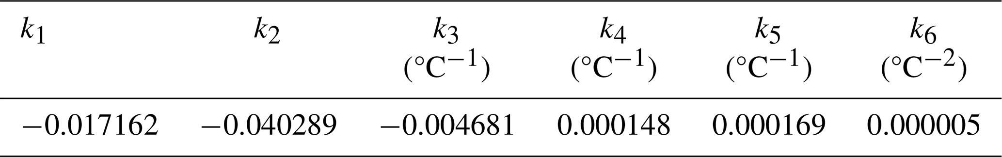
where a_r = 0.159; c₁ = $\frac{\mathrm{4}}{\mathrm{3}\mathit{\pi }}$; c₂ = −0.074; a = −3.47 and b = −0.0594. $k_{\mathrm{1},\mathrm{2},\mathrm{3},\mathrm{4},\mathrm{5},\mathrm{6}}$ are the standard PV performance coefficients given in Table A1 (Huld et al., 2011).

Table A1 Standard PV performance coefficients for polycrystalline silicon module (Huld et al., 2011).

Symbol	Description
θs (°)	Solar zenithal angle
θT (°)	PV tilt angle
Φs (°)	Solar azimuth angle
ΦT (°)	PV azimuth angle
θi (°)	Angle of incidence
ρg	Ground albedo
m	Air mass
G (W m−2)	Global horizontal irradiance
D (W m−2)	Diffuse component of G
BN (W m−2)	Direct normal component of G
GT (W m−2)	Transposed G on a tilted PV plane
$B_{\mathrm{N}}^{\mathrm{T}}$ (W m−2)	Transposed BN on a tilted PV plane
$D_{\mathrm{g}}^{\mathrm{T}}$ (W m−2)	Tilted irradiance that is reflected off the ground
DT (W m−2)	Irradiance computed with the Perez et al. (1990) model
αBN	Angular reflection loss on $B_{\mathrm{N}}^{\mathrm{T}}$
αdg	Angular reflection loss on $D_{\mathrm{g}}^{\mathrm{T}}$
αd	Angular reflection loss on DT
$G_{\mathrm{eff}}^{\mathrm{T}}$ (W m−2)	Total effective irradiance of the PV panel
Tair (°C)	Air temperature
ws (m s−1)	Wind speed
Tmodule (°C)	PV module temperature
$G_{\mathrm{norm}}^{\mathrm{T}}$	Normalized total absorbed irradiance
Tdiff (°C)	Temperature difference
ηrel	relative efficiency
PSTC (W)	Nominal capacity
P (W)	PV power