Laboratory and field assessment of mid-infrared absorption (MIRA) instrument performance for methane and ethane dry mole fractions

Concurrent measurements of methane (CH₄) and ethane (C₂H₆) can be used to identify and separate methane sources, as ethane is present in thermogenic sources (e.g., oil and natural gas) but not in biogenic sources (e.g., agriculture). In this study, we evaluated the performance of multiple Aeris MIRA Ultra instruments (Versions 1 and 2) through controlled laboratory tests and tower-based deployments under field conditions. The systems were modified with an external pump, flow control, a Nafion dryer, and a custom-built auxiliary box to automate the system and transmit near real-time data. We determined the best calibration approach for our application, given practical limitations, to be a full calibration cycle (with ambient and high calibration cylinders) about once per day and an ambient calibration cylinder sampled hourly. Measurement uncertainty was assessed, including the uncertainty due to instrument noise as a function of calibration frequency, uncertainty in the water vapor correction, and cylinder assignment uncertainty. Instrument noise was the dominant source of uncertainty for C₂H₆, while the water vapor correction dominated the CH₄ uncertainty. For Version 2 systems with hourly calibrations and a Nafion dryer with counterflow, the mean total uncertainty, including both systematic errors and noise, of hourly averages was 0.8–3.0 ppb CH₄ and 0.35–0.37 ppb C₂H₆. Laboratory intercomparisons showed network compatibility within 1.2 ppb CH₄ and 0.23 ppb C₂H₆, and a collocated deployment with a NOAA Picarro system agreed within 1.8 ppb CH₄. Instrument noise varied substantially amongst the instruments, with errors reaching up to 11 ppb CH₄ and 2 ppb C₂H₆ for hourly means, with similar variability indicated in a 50 h cylinder test. With appropriate engineering and calibration, the Aeris MIRA Ultra has the potential to distinguish regional methane emission sources in many field settings.

1 Introduction

Methane (CH₄), the second most abundant human-induced greenhouse gas, has an atmospheric lifetime of approximately twelve years and a global warming potential more than 80 times that of carbon dioxide (CO₂) over a 20-year period (Myhre et al., 2013; IPCC, 2023). Its global average mole fraction has increased by a factor of 2.7 since the pre-industrial era with the highest annual growth rate of 17 ppb recorded in 2021 – the largest since direct measurements began in 1983 (WMO, 2022). Despite being an effective target for rapid climate change mitigation on decadal time scales, methane sources and sinks remain poorly constrained from local to global scales due to the wide variety of anthropogenic and natural emissions, which often overlap geographically (Saunois et al., 2020).

Methane is generated through different processes, categorized as biogenic (e.g. rice paddies, landfills, sewage and wastewater treatment, and ruminants), thermogenic (e.g. coal, oil and natural gas), and pyrogenic (e.g. incomplete combustion of biomass and other organic materials), all of which have anthropogenic and natural contributions. Saunois et al. (2020) report that 60 % of global methane emissions are from anthropogenic activities, and about 35 % of anthropogenic emissions are related to the production, transportation, and use of fossil fuels, such as coal, oil, and natural gas. Specifically in the United States (U.S.), the Environmental Protection Agency (EPA) reports that the oil and gas sector contributes to approximately 30 % of anthropogenic methane emissions (Collins et al., 2022).

Top-down studies utilizing atmospheric measurements over the past decade have demonstrated that methane emissions from the oil and gas sector are significantly larger than EPA inventory estimates (Alvarez et al., 2018; Barkley et al., 2023, 2019, 2021; Caulton et al., 2018; Karion et al., 2015; Robertson et al., 2017). This disagreement requires additional data to better characterize methane emissions from U.S. natural gas operations. Ethane (C₂H₆) is the second-most abundant component of natural gas produced by thermogenic processes, after CH₄ (Rella et al., 2015; Schwietzke et al., 2014). In contrast, biogenic methane sources do not co-emit C₂H₆. Therefore, ethane is used as a tracer for fossil fuel based CH₄ emissions. Measuring both CH₄ and C₂H₆ mixing ratios can provide information to characterize sources responsible for measured CH₄ enhancements, especially in regions with co-located thermogenic and biogenic methane sources (e.g. the Denver-Julesburg Basin).

In recent years, commercial laser-based spectrometers have been developed with the capability to measure both CH₄ and C₂H₆ mole fractions at high-temporal resolution (Commane et al., 2023; Defratyka et al., 2021a, b; Roscioli et al., 2015). Commane et al. (2023) reported an intercomparison of three newly developed commercial instruments for CH₄ and C₂H₆ and found that an infrared absorption spectrometer from Aerodyne Research Inc. performed best, but is more difficult to deploy to field sites due to its large size, high power consumption, and high level of expertise required for operation. The Picarro G2210-i was able to precisely measure methane but not ethane, consistent with previous results (Defratyka et al., 2021a). The MIRA (mid-infrared absorption) Ultra Leak Detection system from Aeris Technologies, a spectrometer that performed well for both CH₄ and C₂H₆, with noted difficulties related to water vapor, specific setup requirements, and software problems (Commane et al., 2023).

In this paper, we present the first systematic laboratory assessment of multiple Aeris MIRA Ultra instruments for CH₄ and C₂H₆ measurements and a long-term, tower-based comparison of CH₄ dry mole fractions with National Oceanic and Atmospheric Administration (NOAA) Picarro measurements. In Sect. 2, we describe methods for controlling instrument flow rates, managing water vapor, calibration, and automating the instruments for extended deployments, as well as an approach for estimating the various components of measurement uncertainty. We also describe methods of laboratory tests of multiple Aeris MIRA Ultra instruments and a field comparison at a National Oceanic and Atmospheric Administration (NOAA) site. In Sect. 3, we quantify the measurement uncertainty, and calculate the bias and precision from the laboratory and field tests. Finally, we discuss limitations and implications for future applications in Sect. 4.

2 Methodology

2.1 Methane and ethane sensor description

To measure methane and ethane dry mole fractions, we use MIRA Ultra mobile mid-infrared laser absorption spectroscopic gas instruments from Aeris Technologies Inc, with modifications detailed in this section. The instruments use a compact, pressure-stabilized (240 mbar) and temperature-stabilized (near 42 °C) sensor core with a 60 cm³ multi-pass cell. There are four temperature sensors in various locations in the Aeris unit, including in the cell. These temperatures and the cell pressure are recorded in the datasets. In the wavelength range of the instrument, corresponding to frequencies of 2989.2 to 2988.6 cm⁻¹ there are three methane peaks, and all are weighted equally to determine the CH₄ mole fraction. The scanning wavenumber is extended to 2986.7 cm⁻¹ in order to simultaneously capture C₂H₆.

As the manufacturer upgraded the configurations for this instrument throughout 2024, we assessed and used two versions of the Aeris MIRA Ultra, including up to four instruments concurrently. The original version (Version 1) used a proportional valve downstream of the measurement cell with stainless steel internal tubing. The upgraded version (Version 2) uses an upstream proportional valve with Synflex 1300 internal tubing. The spectrum is locked to the wavelength of a water vapor absorption peak for Version 1, whereas for Version 2, the spectrum lock switches to the methane line when the water vapor is below a threshold (about 1000 ppm). This study focuses primarily on the description of laboratory and field tests using the updated Version 2 of the sensor as it is the main version available commercially.

A portable auxiliary box was constructed and placed upstream of each MIRA instrument to facilitate the use of calibration standards and to provide remote data access (Fig. 1). The sample air passes through a pair of three-way valves (Parker, 091-0094-900) that permits the switching of calibration cylinder air into the sample line. A Raspberry Pi (Model 4B) based control system with custom Python operating code controls the three-way valves on a user-defined schedule. As the Aeris reported time is unreliable, the Raspberry Pi performs daily a Network Time Protocol (NTP) synchronization to set the system time. The system also reads the MIRA data stream and combines it with the current time and the three-way valve states. The data files are periodically uploaded to a remote server for processing.

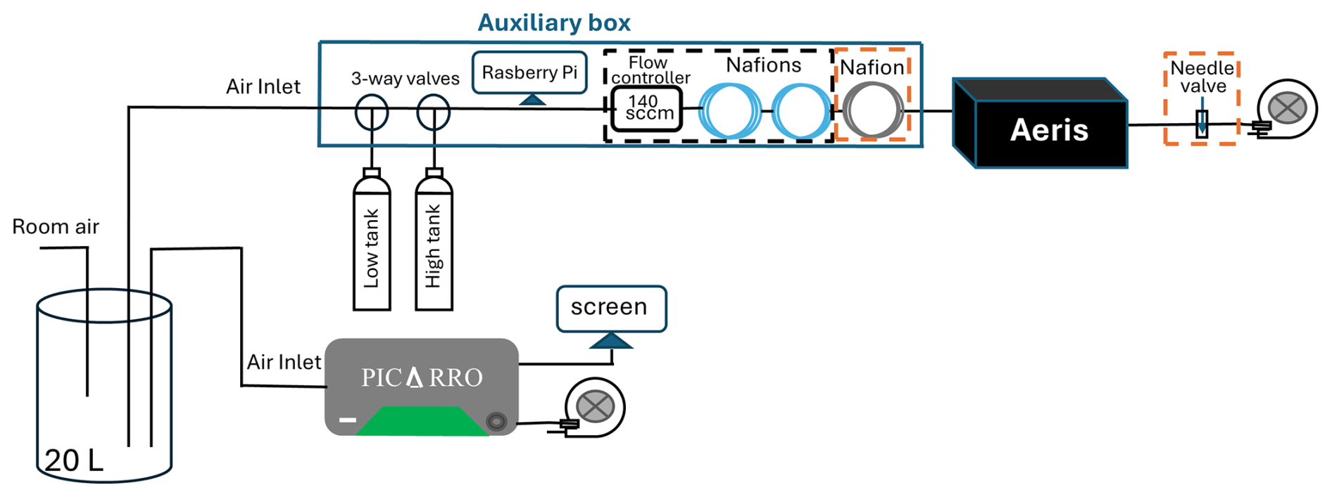
Figure 1 Schematic of the Aeris MIRA Ultra measurement systems for laboratory testing. The components in the black dashed square are included for Version 1 of the Aeris MIRA Ultra and those in the orange dashed square are used for Version 2, while the other components are common to both setups. A total of four identical Aeris systems were measured in parallel for both Version 1 and Version 2 setups.

Sample water vapor, which was regulated to minimize dependence on the water vapor correction, was controlled differently in the two instrument versions. Relatively high mole fractions of water vapor (>5000 ppm) were required to keep the spectra locked on the water line in Version 1 so the typical approach of drying (Andrews et al., 2014) was not possible. To stabilize the water vapor mole fraction and to reduce the dependence on the manufacturer's water correction, we instead minimized the difference of the water vapor mole fractions between the sample air and calibration gases by humidifying the calibration gas to near ambient water levels using two Nafion tube dryers/water exchangers (Perma Pure LLC: MD-070-96S-2 and MD-070-144S-2) without counterflow (Fig. 1). The use of two different dryers/water exchangers was due to availability; a single longer dryer/water exchanger may have achieved the same result. For Version 2 the software did not require high mole fractions of water vapor and thus the sample could be dried to below 2000 ppm H₂O using one Nafion tube dryer/water exchanger (Perma Pure Nafion MD-070-144S-2) with counterflow. Typical differences between the dried sample and the humidified calibration gas, as measured by the Aeris instrument, were 100–500 ppm H₂O.

We engineered methods to control the flow rate of the sample gas, with changes reflecting differences in the two versions of the instrument. The components for Version 1 (Fig. 1) include a mass flow controller set to 140 sccm. The mass flow controller was needed to minimize pressure differences (thought to occur because of the proportional valve being on the outlet rather than the inlet) and to stabilize the water vapor mole fraction when switching between calibration gases and sample air. To simplify field maintenance and minimize the use of calibration gas, the internal pump was disconnected, and an external pump was installed. The flow rate was adjusted from 380 sccm to approximately 140 sccm for laboratory testing and 110–140 sccm for field deployment using a mass flow controller for Version 1. For Version 2, a needle valve was used to adjust the flow rate instead of a mass flow controller (Fig. 1).

2.2 Guidelines for acceptable bias and precision of CH₄ and C₂H₆

We set bias (defined as the long-term mean deviation from the true value) and precision (defined as the standard deviation of hourly differences) guidelines for CH₄ and C₂H₆. In general, network compatibility goals are the maximum instrument biases that can be accepted without adversely affecting model interpretation of gradients (World Meteorological Organization (WMO), 2024: GAW Report No. 292), whereas the total uncertainty contains both bias and random noise. Summertime tower CH₄ enhancements in the Permian Basin averaged around 60 ppb, while wintertime enhancements averaged around 200 ppb (Monteiro et al., 2022). Considering the lower emissions with CH₄ enhancements around 40 ppb in the Denver-Julesburg Basin, a desire for bias less than 10 % of typical network enhancements any time of the year, and instrument capabilities, we adopted a more conservative bias goal of 3 ppb CH₄. The average C₂H₆ to CH₄ ratio is about 5 %–10 % including all biogenic and thermometric methane sources at the Denver-Julesburg Basin area (Daley et al., 2025). Considering also instrument capabilities, we set the corresponding bias guideline for C₂H₆ at 0.3 ppb. We set precision guidelines for the hourly differences (3 ppb CH₄ and 0.3 ppb C₂H₆) to limit the deviations that may impact emissions from inversion modelling on shorter timescales, e.g., weekly. Future instrument improvements allowing further reductions in bias and noise would be beneficial, particularly for regions with lower emissions.

2.3 Laboratory tests

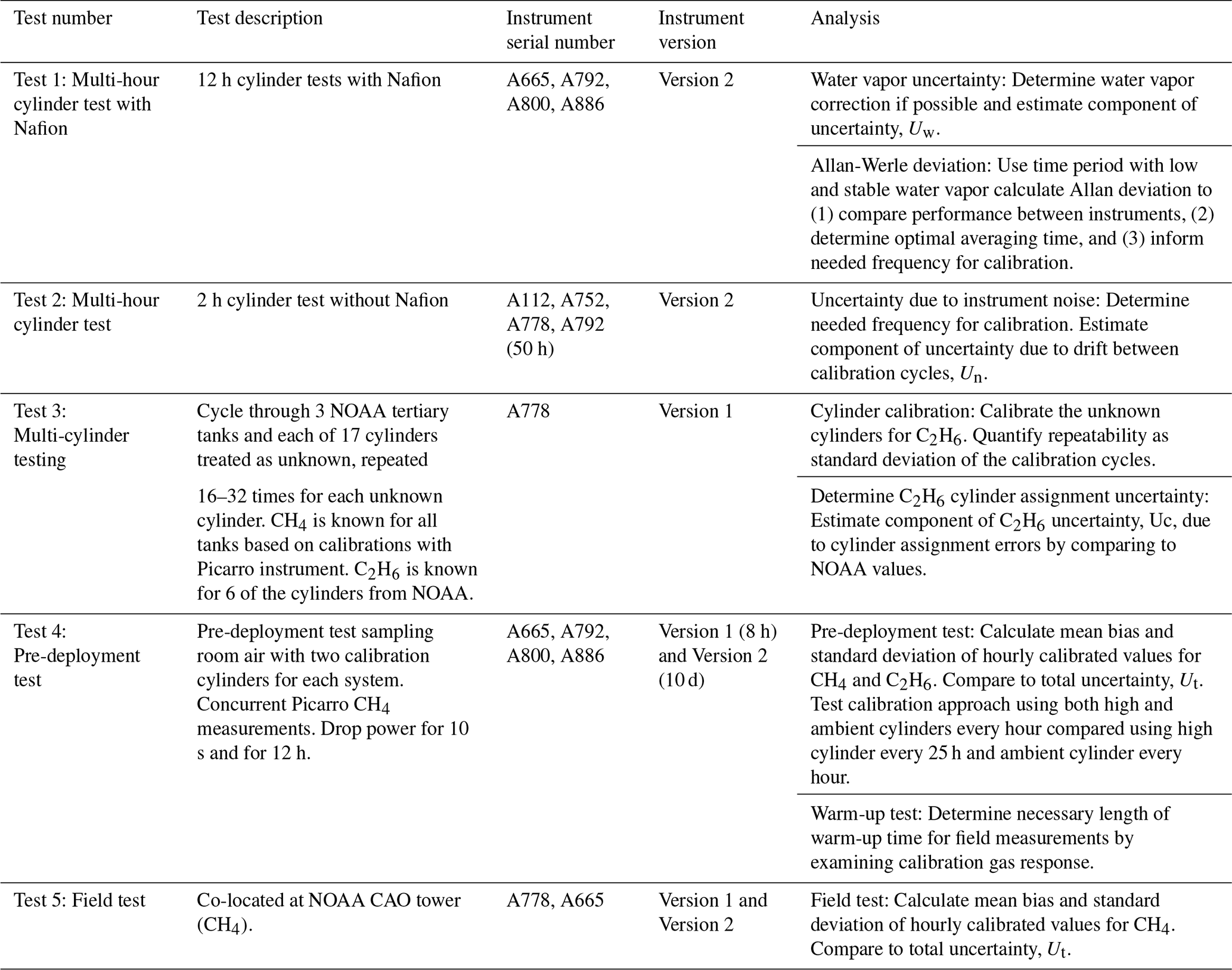
Prior to deployment, we conducted a series of laboratory tests (Tests 1, 2, and 3 in Table 1) to assess the accuracy, precision, and stability of the instruments, to characterize the water vapor response, and to calibrate the field cylinders for C₂H₆. We summarize the methods for these tests below.

Table 1 A summary of the laboratory and field tests.

2.3.1 Multi-hour cylinder tests (Tests 1 and 2)

We tested the manufacturer's water vapor correction of four instruments by sampling a cylinder filled with dry air passing through a humidified Nafion water exchanger (Test 1). Prior to the water vapor dependence test, the membrane inside the Nafion water exchanger was humidified using room air. Then air from a calibrated cylinder with well-known methane and ethane was pulled through the inner tube of the humidified Nafion water exchanger, such that air from the cylinder was humidified to about 0.8 % by volume initially and gradually dried to about 0.02 % over about 12 h. If the water correction was correctly described by a stable relationship in the manufacturer software, the reported CH₄ and C₂H₆ dry mole fractions would not depend on the water vapor level of the resulting air. We performed this test with four instruments (serial numbers A665, A792, A800 and A886, all Version 2 instruments). We used this data to estimate the uncertainty due to an imperfect water vapor correction (method described in Sect. 2.4.1).

We used the same data (Test 1) to compare the noise levels amongst the instruments, to determine the optimal averaging time for calibration cycles, and to inform the needed frequency of calibration by calculating the Allan-Werle deviation as a function of averaging time (Allan, 1987; Werle, 2011; Filges et al., 2015; Shah et al., 2019). To partially separate the effects of instrument noise from variations due to water vapor, we used only the last two hours of data from Test 1 with relatively low and stable water vapor (250–350 ppm H₂O) for these calculations.

To assess the drift of the instruments between calibration cycles, we sampled a cylinder of near ambient values of methane and ethane for a period of just over two days (50 h) using instrument serial number A792 (Test 2). Instrument A792 was selected for this test because its Allan-Werle deviation indicated relatively high variability compared to the other instruments (see Sect. 3.2) so that the results represent the upper end of the expected variability range. The exact dry mole fractions for CH₄ and C₂H₆ of this cylinder were not available, and are not important as we only need a constant sample to assess the drift of the baseline calibration. The cylinder gas was sampled directly so the water was nearly zero. While the Allan-Werle deviation (Test 1) is used to determine the periods at which instrument drift becomes important, it does not quantify the error caused by the drift between calibration cycles. We used data from Test 2 to determine the noise component of uncertainty as a function of calibration frequency (as described in Sect. 2.4.2).

2.3.2 Field cylinder C₂H₆ calibrations (Test 3)

For calibrations of field cylinders with unknown C₂H₆ dry mole fractions, we used one Aeris MIRA Ultra instrument (serial number A778, Version 1) to measure the methane and ethane values of each cylinder (Test 3). The goal of this test was to obtain the most accurate calibrations for the field cylinders possible, so we chose serial number A778 as it exhibited the least noise of the available instruments at the time. We calibrated the Aeris instrument using three NOAA tertiary standards calibrated for methane (1985.9 to 2284.7 ppb) and ethane (1.3 to 22.9 ppb) by the Central Calibration Laboratory (CCL) at the National Oceanic and Atmospheric Administration (NOAA) Global Monitoring Laboratory (GML). The CCL maintains the World Meteorological Organization (WMO) methane scale (WMO X2004A) and an internal CCL standard for ethane (C₂H₆-2012). Several calibration cycles, sampling the NOAA-calibrated tertiaries and the field cylinders in turn, were necessary to average the instrument noise and to determine the repeatability of the calibration values. Of the 17 field cylinders, 11 had unknown C₂H₆ mole fractions, and 6 were calibrated by NOAA CCL but treated as unknown. Each calibration cycle included 4 min for each of three calibrated cylinders and one unknown cylinder (totaling 16 min), with the remainder of the half hour (14 min) sampling room air. Including periods sampling relatively humid room air was necessary as the laser lock was lost if (very dry) calibration cylinders were sampled for an extended period for the Version 1 instruments. Using valves to automate the sequence, the test was repeated for about 8–16 h per field cylinder. The calibration results for the cylinders exhibited instability for several hours before stabilizing. The initial instability occurred for all cylinders and the cause is unknown. Because the cause and period of instability remain unknown and no clear threshold for exclusion could be established, we included all the calibration cycles in Test 3 for transparency and reproducibility. Excluding a consistent number of cycles as warm-up for each cylinder did not appreciably affect the final calibrated cylinder values. The field cylinders were calibrated for CH₄ using a Picarro CRDS as described in Richardson et al. (2017). We also used data from Test 3 to estimate the uncertainty in the assignment of C₂H₆ for the field cylinders (Sect. 2.4.3).

2.4 Uncertainty estimation

The uncertainty of the field observations is a combination of errors in the water correction, drift between calibration cycles (instrument noise), and errors in the mole fractions assigned to each field cylinder (cylinder assignment error). Other factors such as equilibration after gas switching, nonlinearity of the true calibration curve, and changes in the calibration slope on time scales shorter than the time between full calibration cycles (tested in Sect. 3.6.1) are assumed to be small and not included in the uncertainty estimate. We use Tests 1, 2, and 3 (Table 1) to estimate the uncertainty.

2.4.1 Uncertainty due to imperfect water corrections

We used data from multi-hour cylinder tests with Nafion (Test 1) to estimate the uncertainty attributable to imperfect water corrections provided by the manufacturer, despite difficulties in separating water vapor effects from instrument noise. In the field, if the calibration cylinder could be humified to match the water vapor of the dried sample air, the effect of water vapor on the dry mole fractions would be removed by calibration. In practice, there is a difference between the water vapor during calibration cycles and the sample and this difference changes depending on atmospheric humidity and temperature. Using data from Test 1, we determined the slope of the difference between measured and known CH₄ and C₂H₆ dry mole fractions as a function of water vapor for each instrument. The slope for the instrument most sensitive to water vapor (serial number A665) represents an upper bound on the error caused by imperfect water corrections for a given water vapor difference. As an estimate of the uncertainty due to water vapor, U_w, we multiplied the measured water vapor difference in the field at each site as a function of time by this slope.

2.4.2 Uncertainty due to instrument noise

We used data from Test 2 to estimate the uncertainty caused by stochastic drift (instrument noise) in the measurements of Aeris instruments between offset (single cylinder) calibration cycles as a function of calibration frequency. We use the term “stochastic” drift to differentiate the instrument behavior from deterministic drift. Stochastic drift is not random, but does decrease as the averaging time is increased. In the field, the drift between calibration cycles is unknown, but here we simulated offset calibration cycles by continuously sampling from a cylinder for 50 h (Test 2). In the unrealistic case that we calibrate continuously, the error due to drift is zero. We computed two-minute means to mimic the time scale of the calibration cycles in the field. We then simulated calibration cycles by selecting points separated by a range of possible periods between cycles (15 min up to 25 h). We then applied an offset correction, linearly interpolating between the simulated calibration cycles. The error due to instrument drift is the difference between this applied offset calibration between calibration points and the (measured) true behavior of the instrument. We estimate the uncertainty due to instrument noise as the standard deviation of these differences. For reporting the uncertainty in the calibrated dataset, we used these estimates of the instrument noise uncertainty, U_n, with this estimate changing in time as it depends on the calibration frequency used.

2.4.3 Cylinder assignment uncertainty

Our estimate of the cylinder assignment uncertainty (U_c) is based on the uncertainty of the tertiary cylinders used to calibrate the field cylinders and uncertainty of the scale transfer using the Picarro instrument for CH₄ and the Aeris for C₂H₆. The tertiary cylinder uncertainty assigned by NOAA (https://gml.noaa.gov/ccl/refgas.html, last access: 6 October 2025) was 0.1 ppb CH₄. Considering also the uncertainty of the scale transfer, we estimate the cylinder assignment uncertainty for methane based on calibrations using a Picarro instrument to be 0.3 CH₄ based on WMO/IAEA Round Robin Comparison Experiment results (personal communication, NOAA GML). For C₂H₆, we estimate the cylinder assignment error based on the root mean square of the values of the differences between the Penn State and NOAA calibration values (Sect. 3.4).

2.4.4 Total uncertainty

We take the square root of the squared uncertainty components to determine the quadrature sum of the total uncertainty (Eq. 1)

$$\begin{array}{}\text{(1)}& U_{\mathrm{t}}=\sqrt[\mathrm{2}]{U_{\mathrm{n}}^{\mathrm{2}}+U_{\mathrm{w}}^{\mathrm{2}}+U_{\mathrm{c}}^{\mathrm{2}}}\end{array}$$

where U_t is the total uncertainty, U_n is the uncertainty due to the instrument noise, U_w is the uncertainty of the water correction, and U_c is the uncertainty in the field cylinder dry mole fractions.

2.5 Laboratory and field comparisons

We compared the bias and the precision of calibrated hourly dry mole fractions during pre-deployment tests (Test 4) and during a field deployment at NOAA's Colorado Atmospheric Observatory (CAO) (Test 5) to our target compatibility and to the estimated uncertainty.

2.5.1 Pre-deployment tests (Test 4)

To quantify the measurement bias of individual instruments as a proxy for intra-network compatibility, we conducted pre-deployment measurements (Test 4) with four Version 2 Aeris instruments and a Picarro Inc. (model G2301) cavity ring-down spectroscopy (CRDS) instrument (Fig. 1). Picarro instruments are the standard widely used for greenhouse gas monitoring networks (e.g., Yver Kwok et al., 2015). The air inlets for both the Picarro and Aeris MIRA Ultra sampled from an actively-mixed 20 L stainless steel mixing volume. Due to a natural gas leak within the building, the range of methane and ethane was similar those typically measured downwind of oil and gas fields, providing a more thorough test than would background levels. The sampled methane and ethane varied from 2030–2378 ppb CH₄ and 0.3–13.0 ppb C₂H₆ in the laboratory during this 10 d (15–25 November 2024) test. Room temperatures in the laboratory varied by 13 °C throughout the test.

Two high-pressure calibration standard gas cylinders with known concentrations of CH₄ and C₂H₆ were used to calibrate each Aeris system separately, as in the field. We conducted calibration cycles (i.e., measured both ambient and high cylinders – which we refer to as a full calibration cycle) every 3 h. To ensure stabilization after adequately flushing the cell of the instrument, each standard gas was sampled for 4 min continuously, with only the last 2 min of data used to calibrate the instrument using a linear fit.

We compared the hourly calibrated dry mole fractions amongst the four instruments. The mean methane bias, defined as the long-term average of hourly difference between each of the Aeris instruments and the Picarro instrument, was calculated, as well as the standard deviation of the hourly differences. Since no reference instrument was available for ethane, the mean ethane bias and standard deviation was calculated between each instrument and the mean ethane value derived from the four instruments. For the primary intended application of the network of determining regional emissions, intra-network compatibility in the primary concern as only enhancements are utilized, justifying comparison to the mean. Similar tests were performed for four Version 1 Aeris instruments for a period of 8 h. To check if the deviations can be reduced by averaging, we computed biases and standard deviation as a function of averaging time using the ten-day dataset.

Alternative calibration approach: In the data processing, we tested an alternative calibration approach in which we used one full calibration cycle at the beginning of the test, but ignored the subsequent high cylinder results. Following the initial full calibration, we adjusted only the offset using the ambient cylinder every 3 h.

Warm-up tests: As part of the pre-deployment laboratory tests, we performed warm-up tests to characterize the time needed for the instrument to stabilize after a power loss, assessed based on the measurements of the calibration gases. We intentionally interrupted power to all four systems for 10 s by temporarily disconnecting them. Additionally, the instruments were also shut down for 12 h in order to test a completely cold startup.

2.5.2 Field deployment comparison (Test 5)

After laboratory pre-deployment testing, four Aeris MIRA Ultra measurement systems based on Version 1 were deployed in May 2024 forming a tower-based observation network surrounding the Denver-Julesburg Basin (https://sites.psu.edu/saber/, last access: 6 October 2025), a region characterized by methane emissions from both the production of oil and gas and animal agriculture. Four Version 1 instruments were initially deployed at CSU, HUC, JLC, and CAO (Fig. 2). Version 1 instruments were replaced by Version 2 instruments in early 2025.

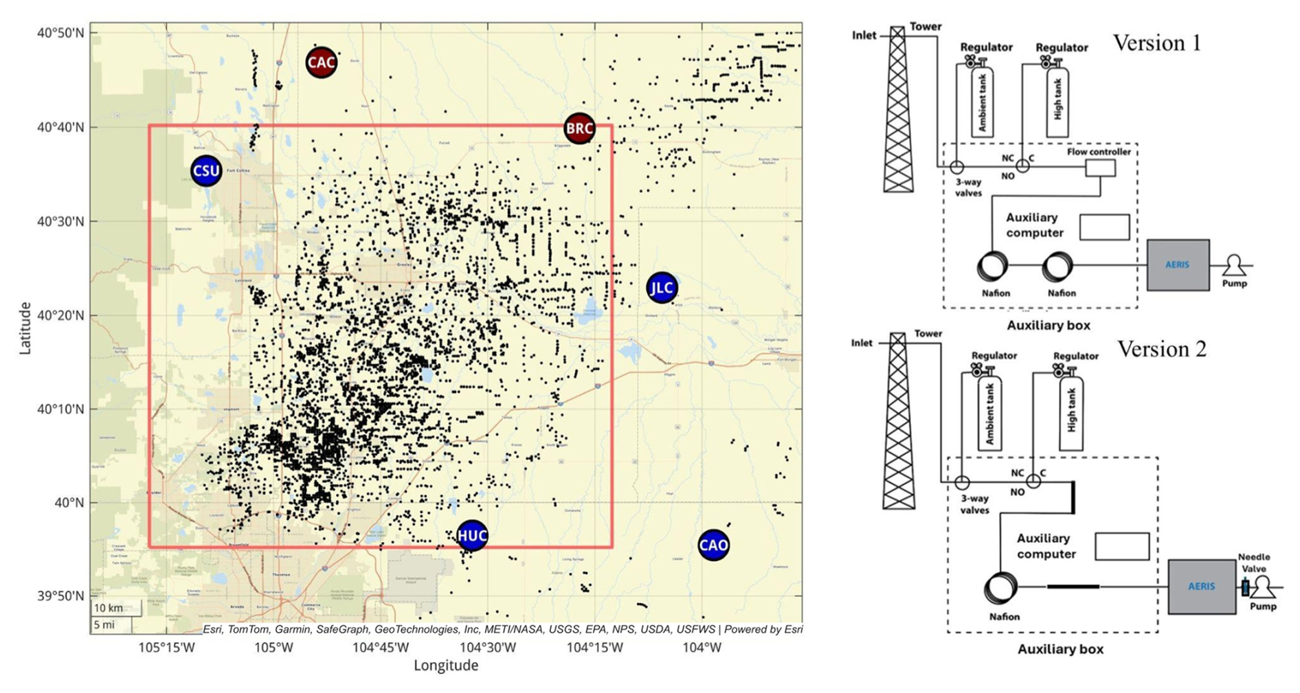
Figure 2 The tower-based network (left panel) and the diagram of the equipment at the tower sites. Active oil and gas sites data during the time of study (https://ecmc.state.co.us/dashboard.html#/dashboard, last access: 2 February 2026) are indicated as black points. As of November 2025, sites CAC and BRC had not yet been deployed. The tower sites were upgraded from Version 1 to Version 2 in early 2025.

Set-up: The NOAA tower site CAO (39.9239° N, 103.9721° W) was chosen for a field comparison with NOAA Picarro CH₄ measurements to assess the bias compared to the calculated total uncertainty. Methane and ethane data from the CAO Aeris MIRA Ultra (serial number A665) were collected starting in June 2024. The Picarro and the Aeris instruments were located in a sea container next to the tower. Since the serial number A665 showed the largest water vapor sensitivity and the most unrealistic deviations among the instruments, we co-located it with the Picarro to rigorously assess the field performance of the Aeris MIRA Ultra methane measurements. The other instruments, which exhibited more stable behavior, should perform better than A665. The tower-based network and the diagram of the field tower setup at CAO is shown in Fig. 2. The NOAA Picarro switched inlet heights (30 m, 100 m, and 479 m a.g.l.) every 5 min with a calibration and sampling protocol based on Andrews et al. (2014). Continuous ethane measurements are not available from the NOAA in situ instrument and flask ethane measurements are collected only at 478 m a.g.l. and thus were not considered for comparison. The NOAA Picarro line was flushed with an additional pump with a high flow rate such that the sample air takes only several seconds (8–14 s) to reach the instrument and the data were reported as 2 min means every 15 min. The Aeris instrument analyzed air from 30 m a.g.l. using a dedicated sampling line. The flow rate for the Aeris was controlled at 110 sccm, using only the pump for the instrument. With this flow rate, the air took about 20 min to travel from the inlet to the Aeris MIRA Ultra. The timing difference was accounted for in the comparison. To minimize noise that might be caused by mismatches in timing, the hours with large atmospheric variability were removed (Levin et al., 2020; Richardson et al., 2012, 2017; Miles et al., 2018). We used a threshold of 7 ppb CH₄ for the standard deviation within each hour above which the data for that hour were excluded (Richardson et al., 2017). This procedure is only applied for the comparison with the NOAA Picarro at CAO. For all field data, we ignored 3 h of data after a loss of power or other restart to allow for the instrument to fully warm up, despite no obvious indicators of problems (Sect. 3.6.1). Additionally, we deployed two Aeris instruments with separate calibration cylinders at CAO for about one month in June 2024.

Calibration frequency changes: The calibration frequency for the Aeris instrument changed throughout the deployment, as the optimal procedure was not determined prior to deployment. For 1 June–31 December 2024, a full calibration cycle (with ambient and high calibration cylinders) was applied every 3 h. For 7 January–8 June 2025, a full calibration cycle was applied every 25 h with an ambient calibration cylinder sampled every 5 h. From 9 June 2025 to the present, a full calibration cycle (with ambient and high calibration cylinders) was sampled about once per day (every 25 h), with an ambient calibration cylinder sampled hourly. We linearly interpolate between hourly offset calibrations.

3 Results

3.1 Water vapor dependence (Test 1)

3.1.1 Errors as a function of water vapor

The Aeris instruments, using the manufacturer-supplied water vapor correction, showed substantial sensitivity to water vapor for measurements of methane and this sensitivity was not consistent between individual instruments. Methane differences from known values varied by more than 50 ppb for serial numbers A665 and A792, and by about 5–10 ppb for A800 and A886 across water vapor levels from 0.02 % to 0.8 % (Fig. 4a), indicating better manufacturer water corrections for A800 and A886. Only A665 and A792 showed linear responses to changes in water vapor mole fraction (Fig. 4a). Testing the application of these linear water vapor corrections to the pre-deployment measurement test (Test 4, Sect. 3.6.1) from 15–25 November 2024 improved the mean biases (between Aeris and Picarro) a moderate amount (from 1.2 to −0.3 ppb CH₄ for A665 and from −1.1 to −0.7 ppb CH₄ for A792). Because of instrument noise and lack of repeated tests, we did not apply these potential water vapor corrections to the laboratory or field data.

The sensitivity of the ethane measurements to water vapor concentration was not clear, possibly because of instrument drift during the experiment. Across water vapor levels from 0.02 % to 0.8 %, ethane errors ranged from −2.8 to 1.6 ppb. Only the result for serial number A665 indicated a trend with R² greater than 0.5. The instrument drift appeared to be larger in magnitude for very low water vapor (less than 0.1 %). The magnitude of the ethane differences from known values was on the same order as the ethane instrument noise (Sect. 3.3), making it difficult to disentangle the cause of the errors.

3.1.2 Uncertainty due to errors in the water vapor correction

The slope of the instrument exhibiting the largest water vapor dependence (serial number A665 in Fig. 3) is 62.7 ppb CH₄/% H₂O and 2.97 ppb C₂H₆/% H₂O. At typical H₂O differences of water vapor between the sample and calibration gas of 100–500 ppm, depending on site, this corresponds to 0.03–0.15 ppb C₂H₆ and 0.6–3.0 ppb CH₄. The error due to water vapor is likely a bias that is instrument specific, but it is possible that it changes in time. For ethane, it is possible that the errors (Fig. 3b) result from instrument noise rather than water vapor effects, but the assigned uncertainty is an effort to capture the range of the possible effect.

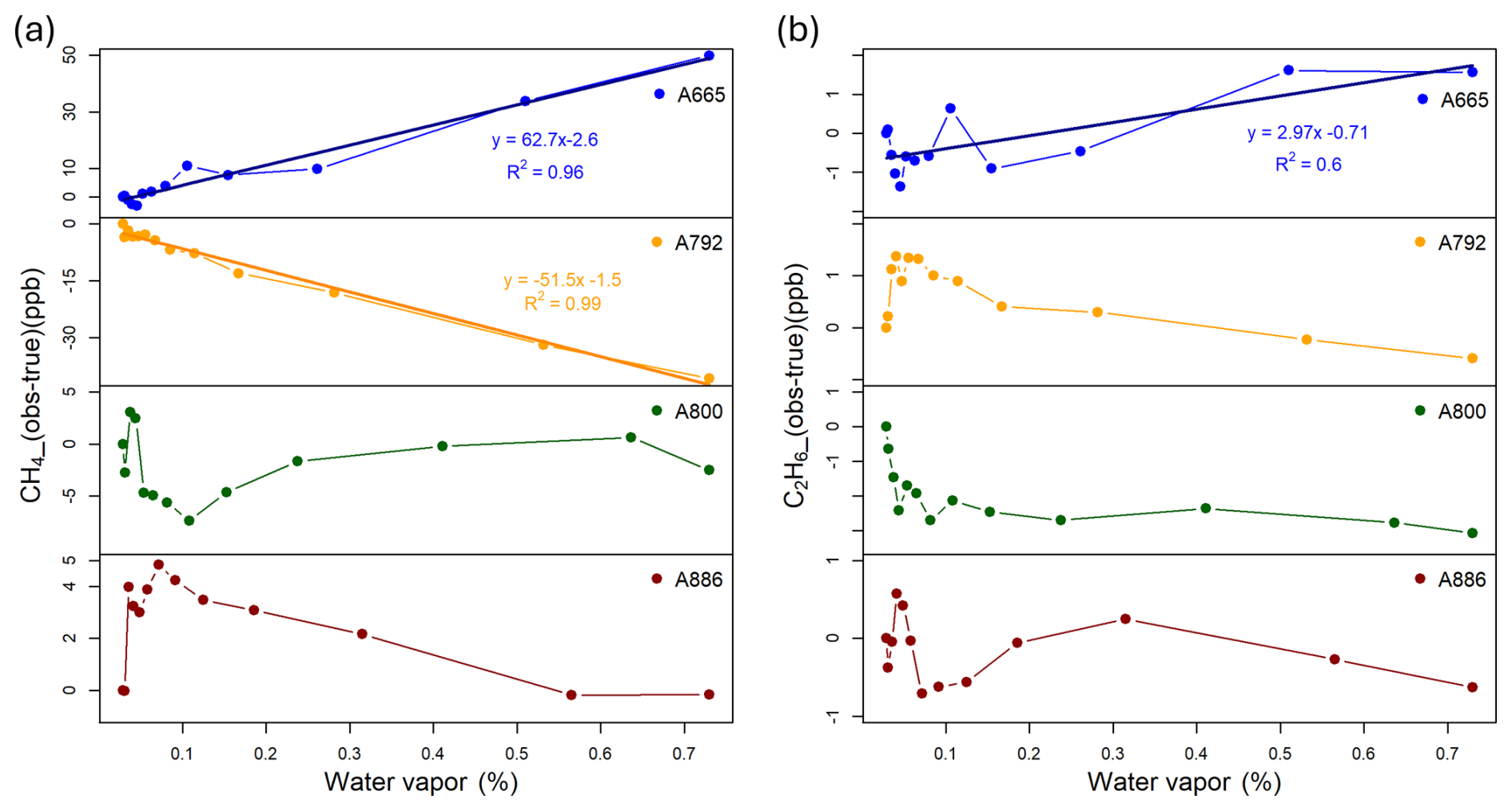
Figure 3 Water vapor dependence laboratory test for methane (a) of the four instruments (the points represent hourly averaged data), with the y-axis indicating pre-calibration measured compared to known CH₄ values. Water vapor dependence laboratory test for ethane (b) of the four Version 2 instruments. The points represent hourly averaged data. Note that without applying any zero or span using the Aeris software, the errors were up to 190 ppb CH₄ and 15 ppb C₂H₆. The data were thus “zeroed” by setting the error at the lowest water vapor value to zero.

3.2 Allan-Werle deviation test (Test 1)

In the calculated Allan-Werle deviations of the instruments, there are significant differences in performance amongst the instruments for both CH₄ and C₂H₆, with the observed Allan-Werle deviation at 1 Hz ranging from 0.7 to 2.1 ppb for methane and from 0.1 to 0.3 ppb for ethane across the four Version 2 instruments (Fig. 4). The Allan-Werle deviation was minimized (0.1–0.3 ppb CH₄ and 0.02–0.04 ppb C₂H₆, depending on instrument) for averaging times 30 s to 2 min, the optimal averaging time for calibration cycles.

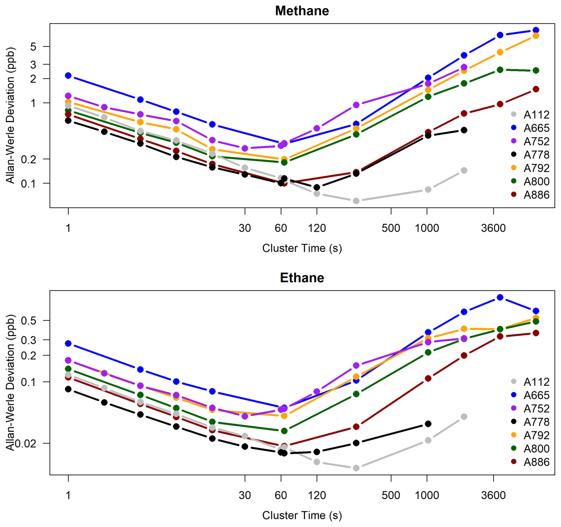
Figure 4 The results of Allan-Werle deviation tests for seven Version 2 instruments, as a function of cluster time. Cylinders with dry mole fractions of about 1980 ppb CH₄ and 1 ppb C₂H₆ were sampled for 12 h with an inline humified Nafion dryer/gas exchanger (for serial numbers A665, A792, A800, and A886). Only the last 2 h, when the water vapor was relatively low and stable (250–350 ppm H₂O), was used for this test. For serial numbers A112, A752 and A778, a cylinder was sampled for 2 h (without Nafion). For serial number A792, the results for the longer 50 h Test 2 (without Nafion) are shown, but the results up to 5 min (300 s) are similar for Test 1. For all the instruments, the retrieved Allan-Werle Deviation (at 1s) is about 0.03 %–0.1 % CH₄ and 10 %–30 % C₂H₆.

For periods larger than the Allan-Werle deviation minimum period, the measurements were affected by drift, suggesting a benefit to calibrating at these timescales, particularly for ethane. For methane, the Allan-Werle deviation was less than 1.4 ppb for periods up to 5 h (18 000 s), so the drift at this timescale is not significant. For ethane however, the Allan-Werle deviation exceeded 0.2 ppb for 17 min (about 1000 s) averaging period and continued to increase (Fig. 4), suggesting a benefit in reducing instrument noise by using a calibration frequency of around 15 min or less, which is unfortunately not practical.

3.3 Uncertainty due to instrument noise as a function of calibration frequency (Test 2)

The errors due to uncorrected stochastic drift (instrument noise) between calibration cycles are a function of calibration cycle frequency (Figs. 5 and 6). The measured CH₄ and C₂H₆ would not have a trend between calibration cycles if the instrument did not drift. Instead, the methane varied between 1993 and 2003 ppb CH₄ and the ethane between 1 and 4.5 ppb C₂H₆ throughout the test (Figs. 5ab and 6ab). The error due to interpolation between 5 h calibration cycles is up to ±4.5 ppb for methane (Fig. 5c) (target compatibility of ±3 ppb) and ±1.5 ppb for ethane (Fig. 6c) (target compatibility of ±0.3 ppb). Thus, the variations of ethane between calibration cycles are almost an order of magnitude larger than the target compatibility. While some periods are relatively stable, others exhibit drift as large as 2 ppb C₂H₆ per hour, necessitating linear interpolation between calibration cycles.

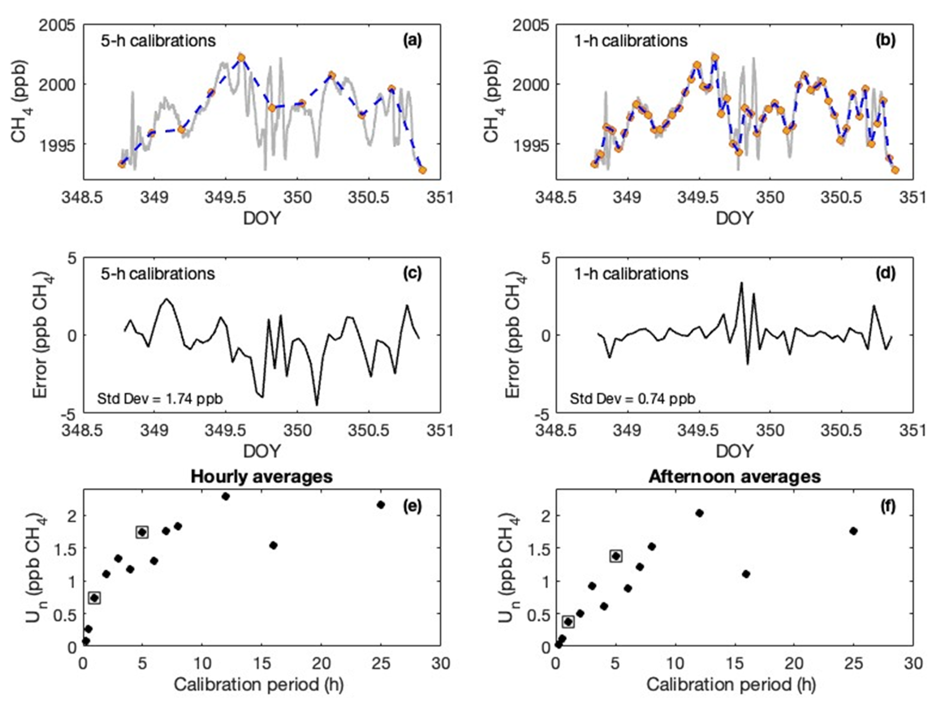
Figure 5 (a–b) Time series of 2 min means of methane (CH₄) (gray line) during a two-day test sampling a cylinder (with essentially no water) for instrument serial number A792. Colored dots indicate examples of (a) 5 h and (b) hourly calibrations. Blue dashed lines indicate linear interpolation between the simulated calibration points. (c) difference between linear interpolation values using 5 h calibration cycles and the observed values. (d) difference between linear interpolation values using 1 h calibration cycles and the observed values. These differences are the error associated with stochastic drift between calibration cycles. The standard deviation of these values (averaged over various values for the beginning point) is indicated. (e) Estimated uncertainty attributable to instrument noise as a function of calibration period for hourly means. (f) Same as (e) but for afternoon (5 h) means. Calibration periods of 1 h and 5 h are highlighted with squares in (e) and (f).

Figure 6 As in Fig. 5, but for ethane.

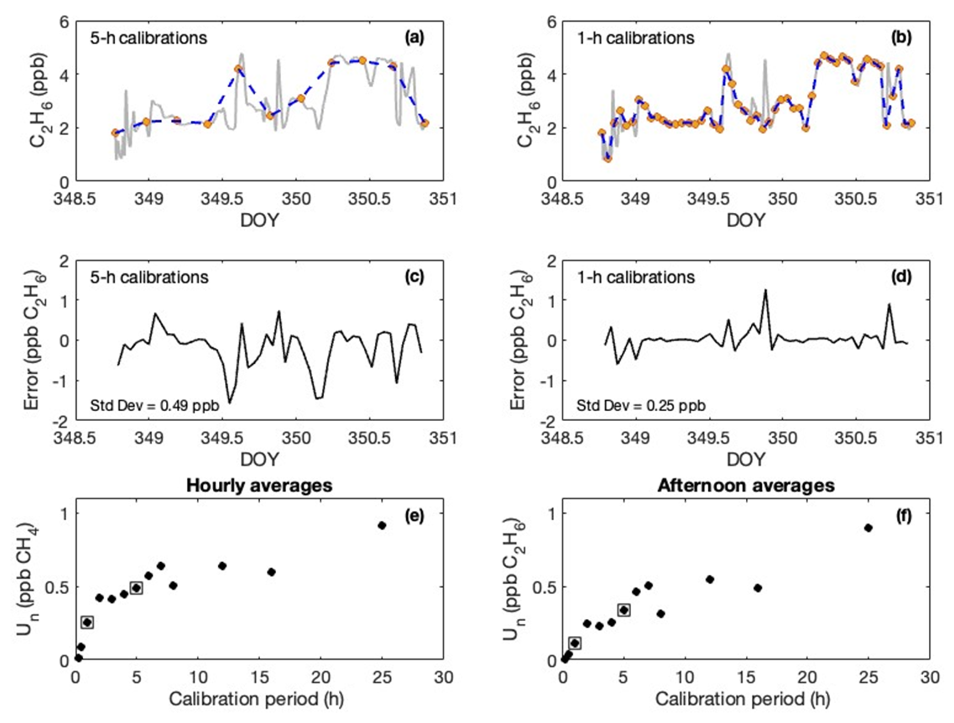
The uncertainty due to noise for ethane is more dependent on the calibration period than for methane, relative to the target compatibility for each species. For example, for calibration cycles separated by 5 h rather than 1 h the uncertainty in the C₂H₆ increases from 0.25 to 0.49 ppb (Fig. 5e). The uncertainty in the CH₄ is less likely to exceed the target compatibility, as it increased from 0.74 ppb (1 h calibration) to 1.74 ppb (5 h calibration) (Fig. 6e). The instrument noise averages out as more data is considered, so the uncertainty due to noise for afternoon averages (Figs. 5f and 6f), for example, is less than that of the hourly values (0.37 ppb CH₄ and 0.11 ppb C₂H₆). The noise is not completely random, however, as it decreases by less than the square root of the number of data points.

3.4 Cylinder calibrations and assignment uncertainty (Test 3)

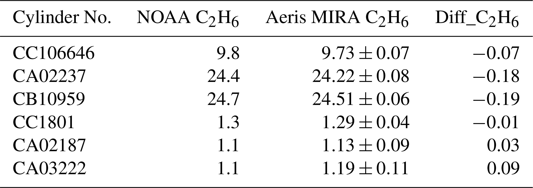
The Aeris MIRA Ultra field cylinder calibrations were between 0.01 and 0.19 ppb C₂H₆ different in magnitude compared to NOAA values (Table 2). The root mean square of these differences was 0.12 ppb C₂H₆, the field cylinder assignment uncertainty. All the calibration curves showed a strong linearity with R² values above 0.99. Extrapolation errors outside of the field calibration range because of non-linearity are thus not likely to be significant. In the field, with only two cylinders utilized to determine slope, field cylinder assignment errors lead to systematically increasing errors outside the range of the field cylinders. For example, if the low cylinder (1 ppb C₂H₆) at a field site is assigned correctly, but the high cylinder at 24 ppb is assigned a value 0.2 ppb C₂H₆ from its true value, the error of an atmospheric sample at 36 ppb is 0.3 ppb.

Table 2 Comparison of the result of the cylinders measured by Aeris MIRA Ultra (Test 3) and NOAA CCL (all in ppb) for the subset of field calibration cylinders with available NOAA C₂H₆ calibrations. Aeris MIRA Ultra (serial number A778) results include the mean value ± standard deviation of the calibration cycles (more than 10 cycles were conducted for each cylinder). Diff_C₂H₆ is the difference between NOAA calibrated values and the Aeris results.

3.5 Total uncertainty

The mean estimated total uncertainty, including that due to errors in the water vapor correction, instrument noise between calibration cycles, and cylinder assignment error, during normal operations (hourly ambient cylinder calibration and nominal drying performance) is 0.8–3.0 ppb CH₄ and 0.35–0.37 ppb C₂H₆, depending on site, for hourly means. During longer times between calibration cycles or less effective drying, the uncertainty is higher, up to 6.1 ppb CH₄ and 0.46 ppb C₂H₆.

3.6 Comparisons (Tests 4 and 5)

3.6.1 Pre-deployment tests (Test 4)

Bias and standard deviation for hourly averages: For the 10 d pre-deployment test, the mean biases for both methane (compared to the Picarro methane mole fraction) and ethane (compared to the mean ethane mole fraction derived from all Aeris instruments) (Fig. 7) are less than or equal to 1.2 ppb CH₄ and 0.23 ppb C₂H₆ (specifically −1.1 to 1.2 ppb CH₄ and −0.22 to 0.23 ppb C₂H₆). The mean biases for methane and ethane were slightly worse, less than or equal to 1.9 ppb CH₄ and 0.24 ppb C₂H₆, for the original version (Version 1) over an 8 h pre-deployment test before the initial field deployment (not shown). When the averaging time for calibrated values is 1 h, the precision (standard deviations of the differences) is 0.6 to 2.3 ppb CH₄ and 0.20 to 0.40 ppb C₂H₆ (Fig. 7, Version 2).

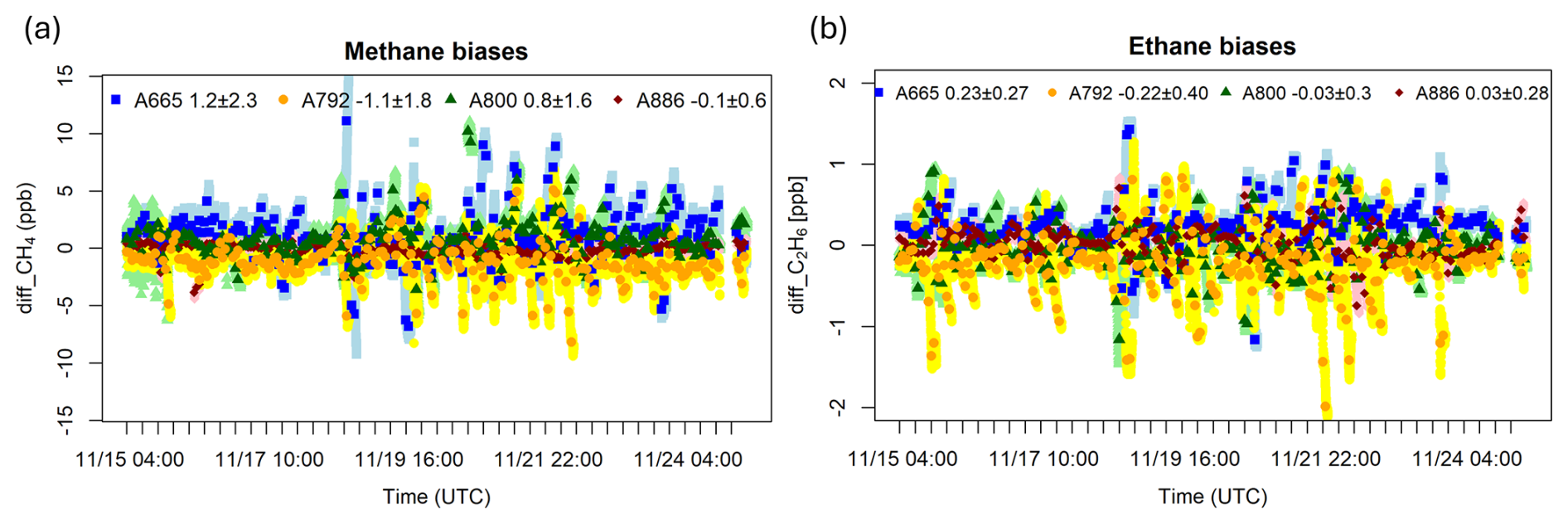
Figure 7 The time series of the Aeris methane mole fractions (a) compared to the Picarro methane mole fraction, and Aeris ethane mole fractions (b) compared to the mean of the hourly ethane mole fraction from all Aeris sensors (Version 2) during the pre-deployment test (15–25 November 2024). Sampled methane and ethane varied from 2030–2378 ppb CH₄ and 0.3–13.0 ppb C₂H₆. Light blue, yellow, light green and pink dots are the minute averaged data respectively for A665, A792, A800 and A886. Blue, orange, dark green and dark red dots are the hourly averaged data respectively for A665, A792, A800 and A886. The data were calibrated by running a full calibration cycle (i.e., both ambient and high cylinders) every 3 h. The numbers on the top represent the mean biases ± standard deviation during the 10 d pre-deployment test.

While the long-term bias and the standard deviations are within the estimated total uncertainty (0.8–3.0 ppb CH₄ and 0.35–0.37 ppb C₂H₆), the variability is higher than desired for some instruments, with individual hourly measurements with much higher errors (up to 11 ppb CH₄ and 2 ppb C₂H₆). These unrealistic deviations occur more frequently for serial numbers A665 and A792. Serial number A886 is the most stable instrument for both methane and ethane with the lowest standard deviation.

Testing of calibration approach: Errors in the initial slope from the manufacturer were significant, but not as large as the offset error. Without applying any offset or slope adjustment using the Aeris software or in post-processing, the errors were up to 190 ppb CH₄ and 15 ppb C₂H₆, depending on the specific instrument. Without an initial full calibration cycle, i.e., using only the ambient cylinder with no slope adjustment from the manufacturer calibration, the mean bias increased to −3.2 to 4.9 ppb CH₄ and −0.34 to 0.19 ppb C₂H₆ and the standard deviation increased to 2.0 to 2.9 ppb CH₄ and 0.24 to 0.44 ppb C₂H₆, depending on instrument, for this 10 d pre-deployment test.

Use of an initial full calibration cycle and only the ambient cylinder offset calibrations every 3 h had little effect on the results compared to using full calibration cycles every 3 h, with mean biases changing by 0–0.4 ppb CH₄ and 0.01–0.02 ppb C₂H₆ and standard deviation changing by less than 0.1 ppb CH₄ and less than 0.04 ppb C₂H₆. This result indicates that the slope of the true calibration curve does not change appreciably in a 10 d timeframe.

Warm-up test: We found no evidence for the need for a warm-up period for the Aeris instruments. When the power was lost for a short time (10 s), we found no effect on the instrument with no warm-up time needed for the warm restart. The cold start results showed that Aeris instruments reported no differences in the standard gases values before and after the instrument restarted and showed the instrument appeared to warm up quickly after restart. The first calibration cycles did not deviate from the subsequent cycles. The slope of the fit was not affected by outages ranging from a few seconds to 12 h during testing.

3.6.2 Field comparison (Test 5)

The magnitude of the differences between the NOAA Picarro CH₄ dry mole fraction and that of the co-located Aeris system differed primarily based on calibration frequency. The Aeris system showed a methane bias of 0.7 ppb CH₄, with a standard deviation of the hourly differences of 2.8 ppb (Fig. 8) for Version 1 with calibrations every 3 h. The performance was considerably worse, with a mean methane difference of 1.4±5.8 ppb during the period when the ambient cylinder was sampled every 5 h (Fig. 9) (Version 2). After changing the calibration of the ambient cylinder from every 5 to every 1 h, the methane differences were less noisy, with a mean bias of 1.8±2.4 ppb, for the version of the instrument and calibration scheme currently deployed in the field. The mean difference of ethane for two independent Aeris systems deployed at CAO for June 2024 was 0.01 ppb C₂H₆ (Fig. S2 in the Supplement).

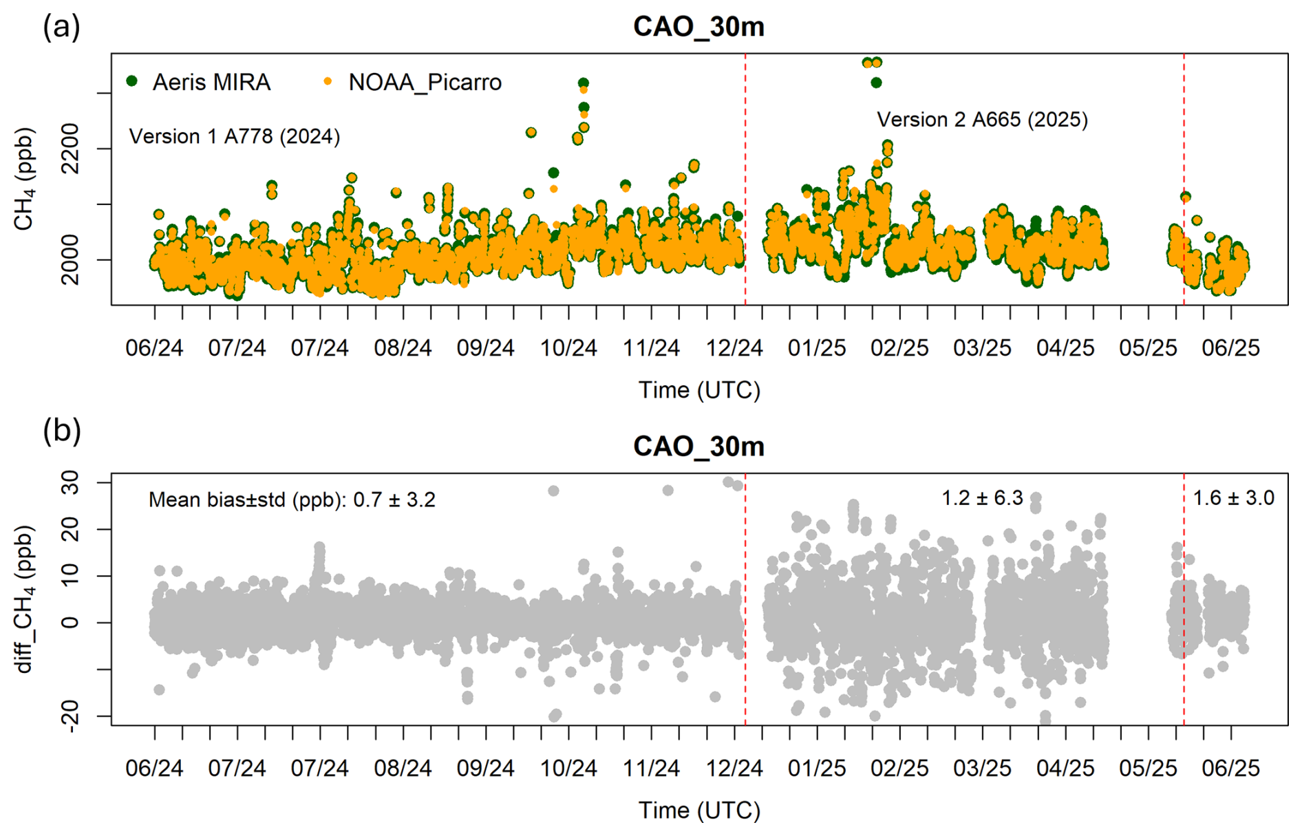
Figure 8 (a) Calibrated hourly methane data from Aeris MIRA Ultra (serial number A665, the instrument with the highest variability indicated by the Allan-Werle deviations in Fig. 4) and NOAA Picarro at 30 m a.g.l. at CAO over the time period of June 2024–June 2025, and (b) the difference between an Aeris MIRA Ultra and NOAA Picarro methane. The hours during which the Aeris' hourly standard deviation or NOAA Picarro's standard deviation was greater than 7 ppb were not included (refer to Sect. 2.5.2). The first red dashed line represents the date on which the instrument was updated from Version 1 (with high and ambient cylinders sampled every 3 h) to Version 2 (with high cylinder sampled every 25 h and ambient cylinder every 5 h). The second red dashed line represents the date on which the calibration period of the ambient cylinder was changed from every 5 h to every 1 h. The high cylinder was always sampled every 25 h for Version 2. The numbers on the top of (b) represent the mean bias ± standard deviation (1σ) over the time periods divided by the red dashed lines. The data gaps were due to a software malfunction of the Aeris MIRA Ultra.

4 Discussion and conclusions

The Aeris MIRA Ultra instruments, with the modifications detailed in this paper, were able to achieve the compatibility goals set for use in determining oil and gas regions via atmospheric inversions. The compatibility (bias) indicated by the pre-deployment tests (better than 1.2 ppb CH₄ and 0.23 ppb C₂H₆) and by the field test at NOAA CAO (better than 1.8 ppb CH₄) are within the target compatibility guidelines (3 ppb CH₄ and 0.3 ppb C₂H₆) (Table 3). The laboratory and field test biases are less than the total uncertainty of the hourly calibrated values (0.8–3.0 ppm CH₄ and 0.35–0.37 ppb C₂H₆), indicating consistency in the results. Instrument noise is the largest component of uncertainty for C₂H₆, whereas water vapor uncertainty is the largest component for CH₄ (Table 3).

The precision (standard deviation) of the hourly calibrated values varied considerably among instruments (0.6–2.3 ppb CH₄ and 0.20–0.40 ppb C₂H₆ during pre-deployment tests; Sect. 3.6.1, Table 3). These results are consistent with the Allan-Werle deviation analysis (Sect. 3.2), which indicated differing levels of instrument noise. Elevated noise in some instruments may complicate interpretation for users relying on a single analyzer.

Table 3 Summary of results under typical conditions (Version 2, hourly offset calibrations and full calibrations every 25 h, and typical drying). The compatibility (bias) guidelines are 3 ppb CH₄ and 0.3 ppb C₂H₆ for the Denver-Jules Basin. Precision is the standard deviation of hourly calibrated differences.

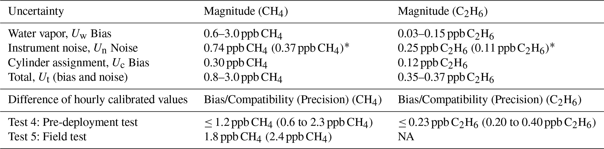
^* Instrument noise is also listed for 5 h (e.g., afternoon) means. Note that the listed water vapor uncertainty for ethane may instead be instrument noise.
NA: not available.

We determined the best calibration approach for our application, given practical limitations, to be a full calibration cycle (with ambient and high calibration cylinders) about once per day (every 25 h), with a more readily available ambient calibration cylinder sampled hourly. Without applying any zero or span using the Aeris software or in post-processing, the errors were up to 190 ppb CH₄ and 15 ppb C₂H₆, depending on the specific instrument. For applications requiring compatibility better than 3 ppb CH₄ and 0.3 ppb C₂H₆, it is essential to use at least one full calibration cycle (using two, or ideally more, cylinders) to correct for slope errors as the magnitude of the bias without adjusting the slope from the manufacturer calibration was up to 4.9 ppb CH₄ and 0.34 ppb C₂H₆. We performed a full calibration cycle every 25 h in the field as protection against potential slope changes in time. Using data from the high cylinders every 3 h instead of only once did not improve the instrument bias or precision in laboratory tests (Sect. 3.6.1). Calibrating less often (high cylinder every 25 h and ambient cylinder every 5 h) in the NOAA CAO field test did not significantly affect the bias but increased the standard deviation of hourly calibrated values from 3.0 to 6.3 ppm (Fig. 8, Sect. 3.6.2).

We observed substantial errors, defined as deviations from the reference instrument for CH₄ and from the mean for C₂H₆, the magnitude and frequency of which depended on the specific instrument (Fig. 7). These errors in hourly-averaged calibrated data were up to 11 ppb CH₄ and 2 ppb C₂H₆ for serial numbers A665 and A792. For ethane, instrument noise poses a significant challenge because background concentrations at tower locations are typically only 0.5–1 ppb C₂H₆. Under these conditions, the noise can periodically result in unphysical negative hourly means, despite hourly calibrations. Since the perturbations are caused by stochastic drift, their impact is reduced in magnitude by increasing the averaging time (Fig. S1). The perturbations may be particularly problematic for non-continuous applications with less data available to average, such as drone-, aircraft-, and vehicle-based analyses.

The uncertainty due to instrument noise, which is larger compared to the target compatibility for ethane than for methane (Sect. 3.3, Table 3), can be further mitigated by considering longer averaging periods. The noise is reduced upon averaging, but not by the square root of the number of measurements as would be expected for random noise (Sect. 3.3 and Fig. S1). For afternoon (5 h) means, with hourly calibrations using an ambient cylinder, the instrument noise uncertainty is quite low, 0.37 ppb CH₄ (Fig. 5f) and 0.11 ppb C₂H₆ (Fig. 6f).

For tower-based inversions with the goal of determining regional fluxes, site-specific long-term bias is more crucial than noise, and the primary potential sources of bias here are cylinder assignment error and uncertainty due to errors in the water vapor correction. Cylinder assignment error is low 0.3 ppb CH₄ and 0.1 ppb C₂H₆, but any errors lead to a site-specific bias. Using more than two field cylinders at each site would likely reduce the effect of assignment error through averaging, and would allow for the ability to independently assess the uncertainty with a target cylinder.

The factory water correction for methane, and possibly for ethane, was not accurate enough for our purposes without partially removing this effect through calibration. Extrapolating the slopes for errors as a function of water vapor (Sect. 3.1) to a typical atmospheric value of 2 %, the errors could be up to 130 ppb CH₄ and 6 ppb C₂H₆ if the sample was not dried at all. We minimized the error by using a Nafion water exchanger to equilibrate the humidity between the sample and calibration gases, as is typically done in similar applications.

Even still, errors in the water correction likely lead to a site-specific bias that is difficult to disentangle given instrument noise and the temperature dependence of the Nafion dryer, and we recommend testing each instrument for water vapor response prior to deployment. We estimate that these biases due to water vapor correction range from 0.6–3.0 ppb CH₄ and 0.03–0.15 ppb C₂H₆ (Table 3, Sect. 3.1.2), for normal conditions, depending on the efficacy of the Nafion dryer and the ambient temperature of the building or shed as well as the manufacturer-supplied water vapor correction of each instrument. Because we only tested the water vapor response of four instruments, it is possible that there is a wider range of responses amongst instruments. In fact, subsequent tests revealed water vapor dependence for methane of double the uncertainty listed here for one instrument (not currently deployed). Ideally the water vapor response would be tested multiple times and an instrument-specific water vapor correction applied if necessary, and repeated tests performed on a regular schedule as it is possible that the true water vapor correction of each instrument changes in time. Future efforts should be focused on testing the water vapor impact on methane and ethane for the water vapor range from 100 to 2000 ppm, which is the typical water vapor range when using a Nafion drier as described here. For future applications, it would be advantageous to quantify instrument-specific noise and water vapor related uncertainty for each individual instrument, and essential if multiple instruments cannot be tested concurrently prior deployment or following any software upgrades.

The impact of these biases on emissions quantification is dependent on the magnitude of the source being measured. For example, since the typical methane enhancements are above 60 to 200 ppb depending on season in the Permian basin (Monteiro et al., 2022) and above 40 ppb in the Denver-Julesburg Basin, a 3 ppb CH₄ bias due to an error in the water vapor correction will have minimal impact on the overall methane emissions calculation. However, the typical methane enhancements in the Indianapolis tower network are about 11–21 ppb for downwind urban sites, depending on the site (Miles et al., 2017). In this latter case, a 3 ppb bias in the instrument measurement can impact the downwind signal by up to 30 %. Because emissions scale linearly with enhancements, this bias in the signal will impact the posterior emission calculation by a similar magnitude. The Aeris MIRA Ultra system may not be a suitable instrument for coverage over regions with modest emission rates, unless the uncertainty is reduced by improving the drying stability between calibration and sample gas, or creating improved water vapor corrections. In low emission areas, rather than quantifying the emissions, such a network would put an upper bound on the emissions that would be consistent with the measurements. For regions with large methane signals, such as the Denver-Julesburg and Permian Basins, the uncertainty for the instrument design presented here is within an acceptable range.

The elaborate and time-consuming procedure used here to calibrate field cylinders for ethane was necessary because the Version 1 instruments lost their line lock after measuring dry air for an extended period of time (∼20 min). This procedure is likely not needed for Version 2 with a software change allowing for line lock to occur using methane rather than water.

The Allan-Werle Deviation results presented here could be improved by separately testing for instrument noise and for water vapor dependence. We thus suggest cylinder tests both with and without an inline Nafion dryer/gas exchanger prior to deployment. The instrument noise is instrument specific and the uncertainty due to noise could be more accurately assessed, rather than using results from one of the instruments with higher noise as an upper bound, as was done here. It is also possible that the instrument noise is a function of mole fraction, either of the analyte, or of water vapor which is used for line locking. Improving the ambient temperature control or that of the cell may also improve the instrument noise performance. And finally the uncertainty could be significantly reduced by developing and applying instrument-specific water vapor corrections, if it can be determined that the function changes slowly enough for this approach to be practical.

The long-term reliability of these instruments in the field is a concern. Problems causing data loss to date include: malfunctioning of the thermoelectric cooler, failure of the sensor boards, inexplicable calibration shifts, solenoid valve or board failure, and unstable serial communication. Some of these issues were solved by power cycling the instruments remotely, but others necessitated physical intervention in the field, in the laboratory, or at the manufacturer.

In conclusion, the tower-based Aeris MIRA Ultra measurement system demonstrated in this study can provide stable and accurate data when carefully configured prior to deployment. The system shows the potential to quantify the ratio between anthropogenic and biogenic methane sources, for regions with mean enhancements of greater than 30 ppb CH₄ and 3 ppb C₂H₆, by providing continuous ethane measurements, assuming the ethane to methane ratio of the sources is known. This capability is particularly valuable in regions such as the Denver–Julesburg Basin, where mixed thermogenic and biogenic methane sources complicate source attribution. More broadly, these instruments can advance our understanding of methane sources and improve our ability to disaggregate greenhouse gas emissions which is an essential step toward informing effective mitigation strategies and addressing the climate crisis.