Optimizing the precision of infrared measurements using the Eppley Laboratory, Inc. model PIR pyrgeometer

The Eppley Precision Infrared Radiometer (PIR) is widely used for broadband (3.5–50 µm), thermal infrared wavelength measurements of the downwelling and upwelling radiation from the atmosphere and surface, respectively. The field of view of the instrument is 2π steradians with a receiver that has an approximate cosine response. In this paper we examine four equations suggested by the literature that have been used to transfer irradiance calibrations from our standard PIRs that are calibrated at the World Radiation Center to field units used for network operations. We first discuss various equations used to convert the resistance measurements of the thermistors to temperatures of the body and dome that are used in the derivation of incoming irradiance. We then use the four related, but distinct, equations for the transfer of the calibration from standard PIRs to field instruments. A clear choice for the preferred equation to use for calibration and transfer of calibration to field PIRs emerges from this study.

1 Introduction

The Eppley Precision Infrared Radiometer (PIR) is a pyrgeometer developed to measure broadband (3.5–50 µm) thermal infrared (hereafter, IR) radiation emitted by the atmosphere and surface. Detecting even small changes in atmospheric and surface IR in the environment are important to understand as they may indicate temperature changes in the environment caused by changes in the atmospheric composition or cloud cover.

The PIR originally came equipped with a battery-powered circuit to compensate for the radiation emitted by the body so the net signal from the instrument was a measure of actual incoming IR radiation. Users of this instrument that are interested in the optimum precision in their IR measurements do not use the battery-powered circuit, but, instead, use temperatures from two thermistors connected to the body and dome of the instrument along with the thermopile output to calculate the incoming IR irradiance signal.

Figure 1 illustrates the most significant incoming and outgoing IR irradiances at the thermopile surface. To derive L, the incoming IR radiation from the hemisphere outside the instrument, radiative equilibrium of the instrument must be defined. To do that, the sum of the incoming radiation transmitted through the dome (labeled 1), radiation emitted by the dome to the receiver (labeled 2), and the radiation emitted by the thermopile surface and reflected by the dome (labeled 3) are set equal to the radiation emitted by the thermopile surface (labeled 4, which is the largest of the IR signals). Note that the dome transmits IR radiation between 3.5 and 50 µm, however, the transmission is not perfect, nor uniform. Considering these components Albrecht and Cox (1977) formulated Eq. (1) for the externally received radiation as

$$\begin{array}{}\text{(1)}& L=U_{\mathrm{thermopile}}\left(c_{\mathrm{1}}+c_{\mathrm{2}}{T}_{\mathrm{B}}^{\mathrm{3}}\right)+{\mathit{\epsilon }}_{\mathrm{o}}\mathit{\sigma }{T}_{\mathrm{B}}^{\mathrm{4}}-k\mathit{\sigma }\left(T_{\mathrm{D}}^{\mathrm{4}}-T_{\mathrm{B}}^{\mathrm{4}}\right),\end{array}$$

where U_thermopile is the voltage measured across the thermopile, T_B and T_D are the body and dome temperatures in K, σ is the Stefan-Boltzmann constant, ε_o is the emissivity of the detector, and c₁, c₂, and k are constants to be determined in calibration.

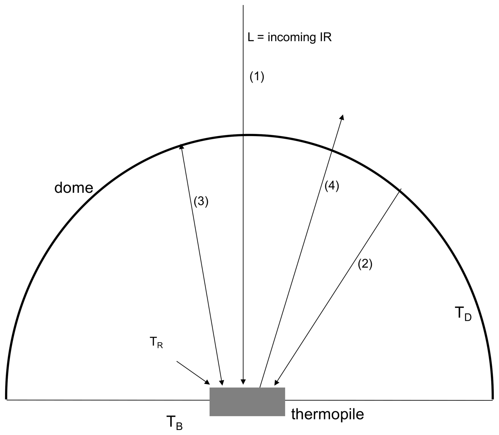
Figure 1 Schematic for the most significant incoming and outgoing IR radiation components on the thermopile surface (numbered 1–4) that are considered in calculating the incident atmospheric IR irradiance. The top of the dark rectangle is the receiving surface surrounded by the dome that transmits IR in the range 3–50 µm. YSI 44031 thermistors are used to measure T_B of the body (thermistor buried in the brass body of the PIR) and T_D of the dome in K. T_R is the estimated receiver temperature in K.

In practice Albrecht and Cox (1977) dropped the $c_{\mathrm{2}}{T}_{\mathrm{B}}^{\mathrm{3}}$ term as negligible relative to the c₁ term and set the emissivity of the body of the instrument ε_o to 1 yielding this commonly expressed form of their equation

$$\begin{array}{}\text{(2)}& L={\displaystyle \frac{U_{\mathrm{thermopile}}}{C}}+\mathit{\sigma }{T}_{\mathrm{B}}^{\mathrm{4}}-k\mathit{\sigma }\left(T_{\mathrm{D}}^{\mathrm{4}}-T_{\mathrm{B}}^{\mathrm{4}}\right),\end{array}$$

where c₁ has been replaced by $\mathrm{1}/C$.

Philipona et al. (1995), however, used Eq. (1) in its entirety, but to compare symbolically to Eq. (2) it is written

$$\begin{array}{}\text{(3)}& L={\displaystyle \frac{U_{\mathrm{thermopile}}}{C}}\left(\mathrm{1}+k_{\mathrm{1}}\mathit{\sigma }{T}_{\mathrm{B}}^{\mathrm{3}}\right)+k_{\mathrm{2}}\mathit{\sigma }{T}_{\mathrm{B}}^{\mathrm{4}}-k_{\mathrm{3}}\mathit{\sigma }\left(T_{\mathrm{D}}^{\mathrm{4}}-T_{\mathrm{B}}^{\mathrm{4}}\right),\end{array}$$

where the $T_{\mathrm{B}}^{\mathrm{3}}$ term in Eq. (1) is retained, the emissivity of the body is k₂, and k₃ is the same as k in Eq. (2). All constants, C, k₁, k₂, and k₃, are determined in calibration.

Payne and Anderson (1999) used the functional form of Eq. (2), but substituted T_R for the T_B, where T_R is the empirically calculated approximate temperature of the receiving surface rather than the measured body temperature as illustrated in Fig. 1. Thus,

$$\begin{array}{}\text{(4)}& L={\displaystyle \frac{U_{\mathrm{thermopile}}}{C}}+\mathit{\sigma }{T}_{\mathrm{R}}^{\mathrm{4}}-k\mathit{\sigma }\left(T_{\mathrm{D}}^{\mathrm{4}}-T_{\mathrm{R}}^{\mathrm{4}}\right).\end{array}$$

Payne and Anderson (1999) estimated T_R using Eq. (5)

$$\begin{array}{}\text{(5)}& T_{\mathrm{R}}=T_{\mathrm{B}}+\mathrm{0.694}\cdot U_{\mathrm{thermopile}},\end{array}$$

where U_thermopile is in millivolts, and the emissivity ε_o is set to unity.

Reda et al. (2002) used a form similar to Eq. (4)

$$\begin{array}{}\text{(6)}& L=k_{\mathrm{0}}+{\displaystyle \frac{U_{\mathrm{thermopile}}}{C}}+k_{\mathrm{2}}\mathit{\sigma }{T}_{\mathrm{R}}^{\mathrm{4}}-k_{\mathrm{3}}\mathit{\sigma }\left(T_{\mathrm{D}}^{\mathrm{4}}-T_{\mathrm{R}}^{\mathrm{4}}\right),\end{array}$$

where the instrument body emissivity k₂ is derived during calibration and a constant term k₀ is introduced. T_R is nearly the same as Eq. (5) with 0.704 replacing the constant 0.694. In this paper we drop the constant term k₀ since there is no physical justification for including it.

Since there are four versions of the original Albrecht and Cox (1977) Eq. (1), this paper attempts to determine which version is best, in the precision sense, to use for PIR calibration transfer, and general use in converting PIR measured quantities to physical units. The organization of this paper is as follows. Because accurate internal thermistor temperatures are critical to pyrgeometer IR measurements, we first examine various versions of the standard cubic equation used to convert the YSI 44031 thermistor resistance to the temperatures of the PIR body and dome. We then calibrate six test PIRs by transferring the calibrations of our three standard PIRs that were in turn calibrated at the World Radiation Center (WRC) in Davos, Switzerland, using the World Infrared Standard Group (WISG). Comparisons are then made between the mean irradiance of the three standard PIRs and the computed irradiance from the test PIRs using the four different forms of the original Albrecht and Cox (1977) formula, i.e., Eq. (1) to calibrate each. Boxplots are used to demonstrate the level of agreement between the standard PIRs and test PIRs for the various formulations. Lastly, a clear conclusion with regards to the preferred technique to use for calibrations and field measurements is suggested.

2 PIR Temperature Measurements

The body and dome temperatures in the Eppley PIR pyrgeometer are measured using the YSI 44031 thermistor. The YSI company provided a table of resistance versus temperature at one K resolution. To get a finer resolution, a mathematical fit to the tabulated data is required. Steinhart and Hart (1968) found that a cubic fit of inverse temperature to the log of measured resistance matched many of the manufacturer's thermistor data points over a wide temperature range. Their equation is

$$\begin{array}{}\text{(7)}& \mathrm{1}/T=a+b\cdot \ln \left(R\right)+c\cdot (\ln R{)}^{\mathrm{2}}+d\cdot (\ln R{)}^{\mathrm{3}},\end{array}$$

where T is the temperature in K and R is the measured resistance in ohms or kiloohms. Note that in the standard Steinhart-Hart equation, the c is set to zero. Coefficients a, b, and d differ depending on whether ohms or kiloohms are used, and on the temperature range over which the fit is made.

Figure 2 is a plot of six independently-derived fits to the same manufacturer's YSI 44031 thermistor data, and Table 1 lists the coefficients of Eq. (7) for those fits. The y-axis is the temperature estimate based on the fit minus the tabulated thermistor data to which the fit is made. The least-squares fit to Eq. (7) (no quadratic term) is indicated by the red line if ohms are used. If a full cubic relationship, including a quadratic term, is used to fit the tabulated data in kiloohms, then similar, but not identical, agreement to the red line is obtained (blue-white line). Interestingly, fitting the full cubic relationship to either ohms or kiloohms yields identical results (again, note the blue-white line). This is not the case if the quadratic term is not included in the fitting to ohms versus kiloohms as discussed in the appendix. Two gray fits in Fig. 2 are from the Baseline Surface Radiation Network (BSRN) – Operation Manual Version 2.1 (McArthur, 2005), and use YSI 44031 resistance in ohms. That published equation yields the bottom gray curve that is displaced from the main grouping in Fig. 2. If their coefficient a is modified slightly from the published 0.0010295 to 0.0010293, as shown in the legend, then an improved fit (upper gray curve) is obtained that agrees well with the others. The green curve, used by the World Radiation Center (WRC) in Davos, Switzerland, was fit over a −30 to +40 °C range, but does well over the entire range of −50 to 50 °C considered here. Differences among the various fits in Fig. 2 are small. All but the bottom gray fit in Fig. 2 cause less than 0.1 W m⁻² of uncertainty in the irradiance estimate.

Table 1 Coefficients for Eq. (7) for lines plotted in Fig. 2.

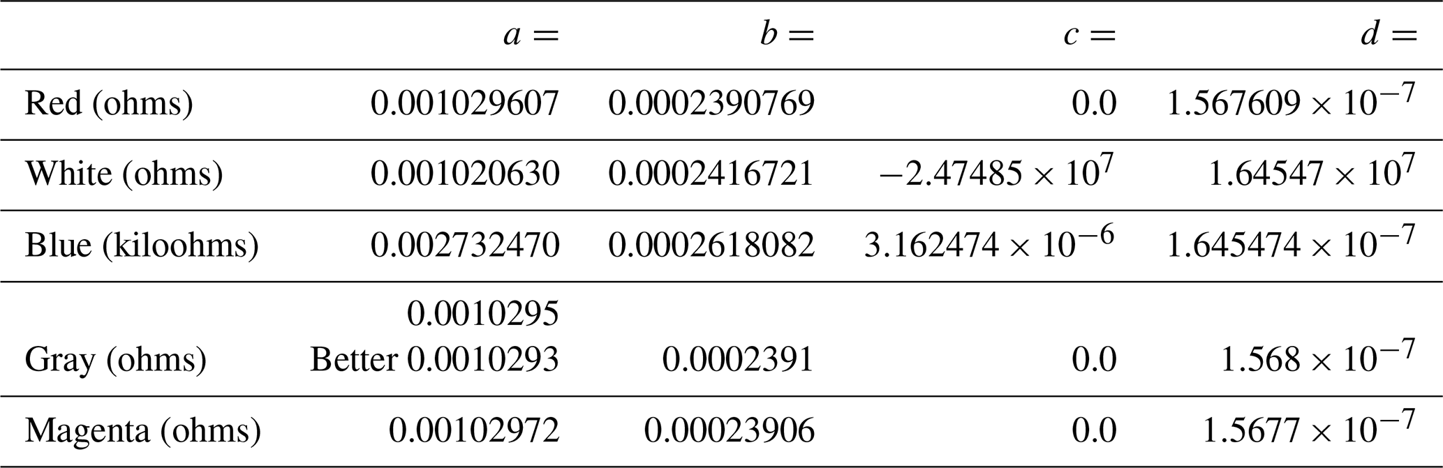
The larger uncertainty in thermistor temperature measurements is the fundamental accuracy of the thermistors used in the PIR, which are specified to be replaceable to 0.2 K. At 300 K, a difference of 0.2 K is a little over 1 W m⁻². In this paper the full cubic (blue-white curve) is used to compute PIR temperatures in the analyzed data.

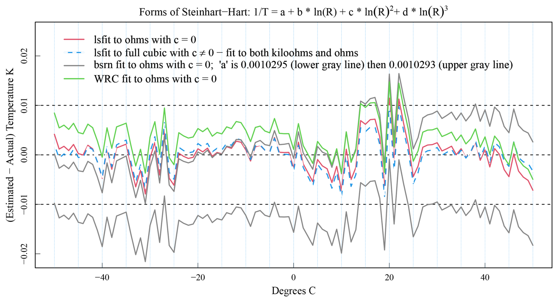
Figure 2 Six independent fits using forms of Eq. (7) to the YSI 44031 tabulated data after subtraction of the tabulated data over the range −50 to 50 °C in 1 °C increments. Similar agreement among all fits ensues if the small change to the published BSRN constant a is made.

The full cubic fits (blue-white line) overlap whether ohms or kiloohms are used (with different coefficients, of course).

3 Four Methods of PIR Calibration Transfer

In this section, we examine the performance of Eqs. (2), (3), (4), and (6) in transferring calibrations from our three “standard” PIRs to field PIRs. Our standard PIRs were calibrated against the world reference (https://www.pmodwrc.ch/en/world-radiation-center-2/irs/wisg/, last access: 3 February 2026) in 2018, 2022, and 2024 at the WRC, which is part of the PMOD in Davos, Switzerland. Each standard was returned with two sets of coefficients, one set for Eq. (2) and one set for Eq. (3). The WRC calibration of our standard PIRs uses their blackbody over a range of pyrgeometer and cavity temperatures to determine the k_i's in Eq. (3). The C determined by this regression is not used, but is set using clear and stable skies outdoors.

To transfer the standard PIRs' calibration to field radiometers, our WRC-calibrated standard PIRs and test PIRs are arranged side-by-side for a week or more on an outdoor horizontal observing platform, with no significant obstructions surrounding the platform. Note that all calibration coefficients of Eqs. (2) and (3) for our test PIRs are obtained by regression analysis, i.e., we used no blackbody for calibration transfer. For this paper two calibration periods and three PIRs from each are analyzed. However, all figures for this paper only display results from the 2023 calibration performed at Table Mountain near Boulder, Colorado USA. Diurnal variability shown in Fig. 3 (top) indicates length of time and the type of conditions used for calibration. On the left are the three standard PIR's outputs with the WRC's Philipona et al. (1995) coefficients applied. On the right are the same standard PIR's with the WRC's Albrecht and Cox (1977) coefficients applied. Agreement among the three on the left is very good because the last-plotted PIR readings (green) overplot the first two (black and red). Agreement on the right is nearly as good but with some underestimation by PIR 32909F3 (red dots). Histograms in Fig. 3 (bottom) indicate the degree of agreement among our standard PIRs more clearly with closer agreement among the results using the Philipona et al. (1995) coefficients.

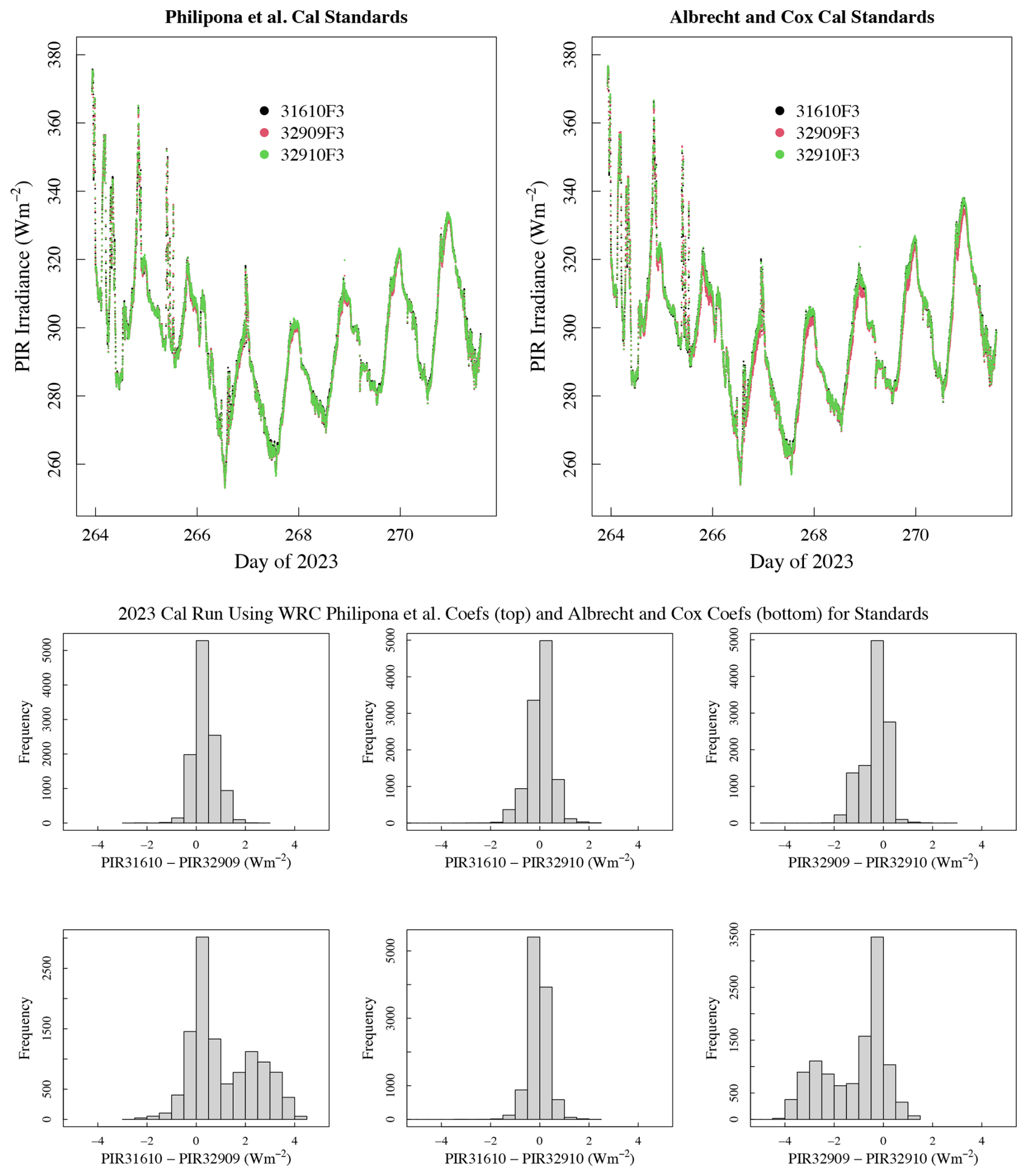
Figure 3 (Top) Calculated IR irradiance from our three standard PIRs (serial numbers in the legend) using Philipona et al. (1995) coefficients provided by WRC are overplotted on the left and the Albrecht and Cox coefficients are used for plot on the right. (Bottom) Histograms of the differences among our standard PIRs applying either the Philipona et al. (1995) WRC-assigned calibration coefficients (upper histograms) or the Albrecht and Cox (1997) WRC-assigned coefficients (lower histograms). Clearly, there is closer agreement in the upper row.

Before comparing results from Eqs. (2), (3), (4), and (6), we first compare results from only Albrecht and Cox (1977, Eq. 2) and Philipona et al. (1995, Eq. 3) for which the WRC provided both sets of coefficients. In this test, the mean IR irradiance of the three standard PIRs is compared to computed IR from a test PIR that was calibrated using the mean of these standard PIRs. The least-squares fitting technique to determine the calibration coefficients for the test instrument uses a robust function in the R language (MASS::rlm) that de-weights outliers to reduce the effects of noisy, for example, rain-contaminated, and other outlier data. As we shall discuss in the final section, this appears to be comparable to the strict criteria used at the WRC for calibration transfer. However, it should be noted that days with known rain events are removed from all test data sets before a calibration transfer is attempted.

In Fig. 4, boxplots are used to compare the performance of the two calibration methods applied to the standard PIRs at the WRC, i.e., Albrecht and Cox (1977) and Philipona et al. (1995). The “box” in these plots contain 50 % of the data, and the lines extending from the top and bottom of the box, or “whiskers,” include about 95 % for normally distributed data. In the top-left panel of Fig. 4 the three standard PIRs use the WRC-provided Albrecht and Cox (1977) coefficients, and the average of the three standard PIRs is compared to coincident test PIR (SN 23215F3) data, also calculated using Albrecht and Cox (1977). The boxplot summarizes those differences over the entire calibration period for PIR 23215F3. The boxplot on the top right summarizes differences following the same procedure, but using Philipona et al. (1995) coefficients for the standard PIRs (WRC-provided) and for the test PIR. Comparing the top panels of Fig. 4, the one on the right, where Philipona coefficients are used exclusively, has a smaller box, shorter whiskers, and a median nearer to zero compared to the panel on the left where Albrecht and Cox was used exclusively.

The bottom panels of Fig. 4 show the same comparison for a different test PIR (SN 38805F3). The same comments apply, with the Philipona et al. (1995) calibrated data (bottom right) giving smaller spread in the box and whiskers, and the median nearer zero, while there is more spread in the bottom-left panel where Albrecht and Cox (1977) is used. Differences in the lower panels of Fig. 4 are generally greater than those in the top panels. The calibration data for these two test instruments were collected concurrently, which suggests that the disparity arises from inherent characteristics of the instruments themselves. We studied a total of six instruments from two distinct calibration periods in this way and found that in every case using the Philipona et al. (1995) form (Eq. 3) gave better results than the formulation of Albrecht and Cox (1977, Eq. 2).

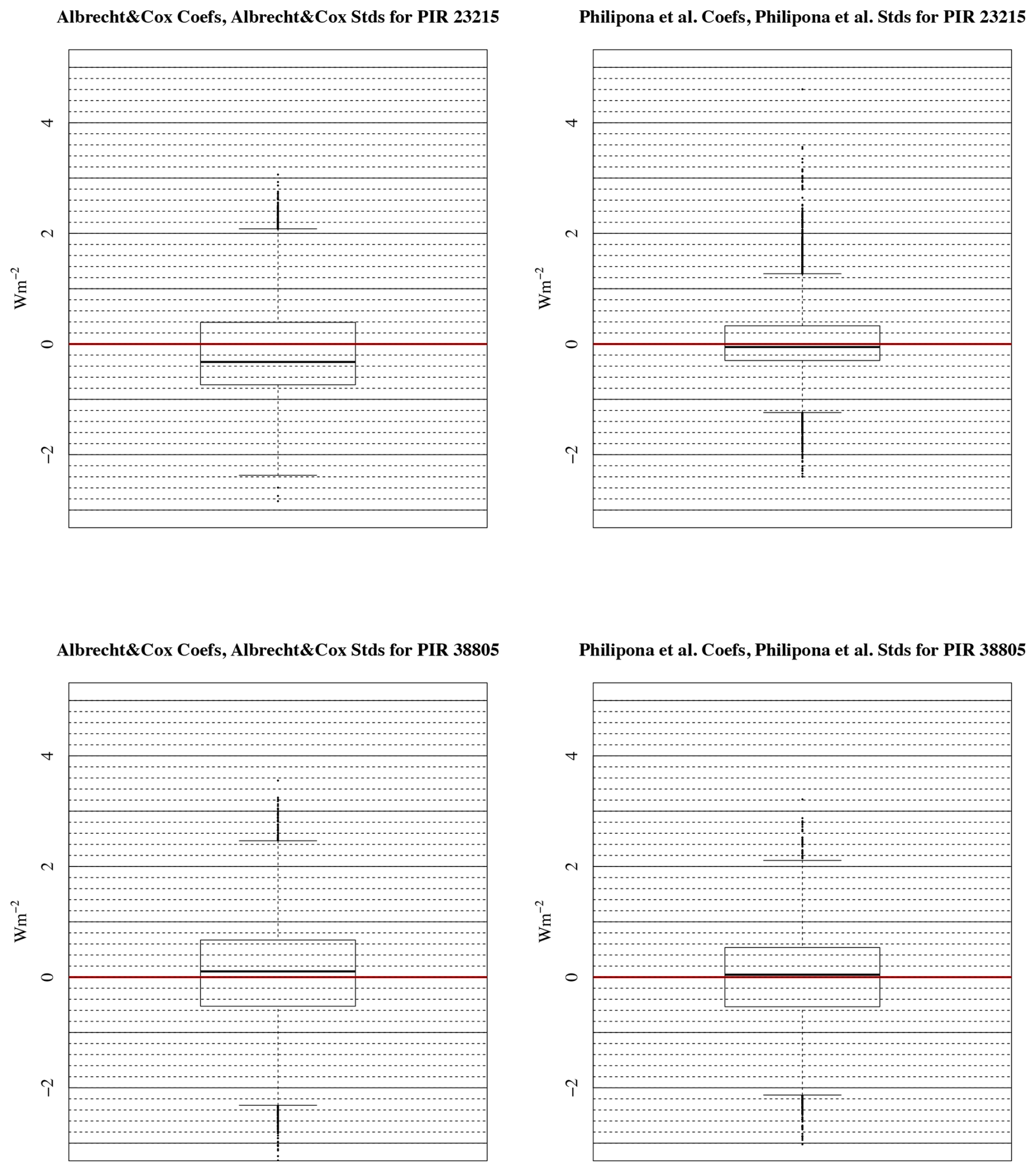
Figure 4 (top) Boxplots of the differences between applying Albrecht and Cox (1977) calibrations and applying Philipona et al. (1995) calibrations for PIR 23215. Note the differences in box widths, whisker lengths, and median values. (bottom) Boxplots for a different PIR (38805) that was calibrated at the same time as the one in Fig. 4 (top).

Next, we compare results from all four Eqs. (2), (3), (4), and (6) for the same two PIRs as in Fig. 4. Since Fig. 4 suggests that the Philipona et al. (1995) Eq. (3) produces better results than Albrecht and Cox (1977) Eq. (2), we use Philipona et al. (1995) coefficients provided by WRC to compute IR irradiance for the standard PIRs and average these as “truth” for all of the comparisons. For both test PIRs in Fig. 5 (top and bottom) the last boxplot on the right (Philipona et al., 1995) gives the best results followed by the adjacent boxplot (Reda).

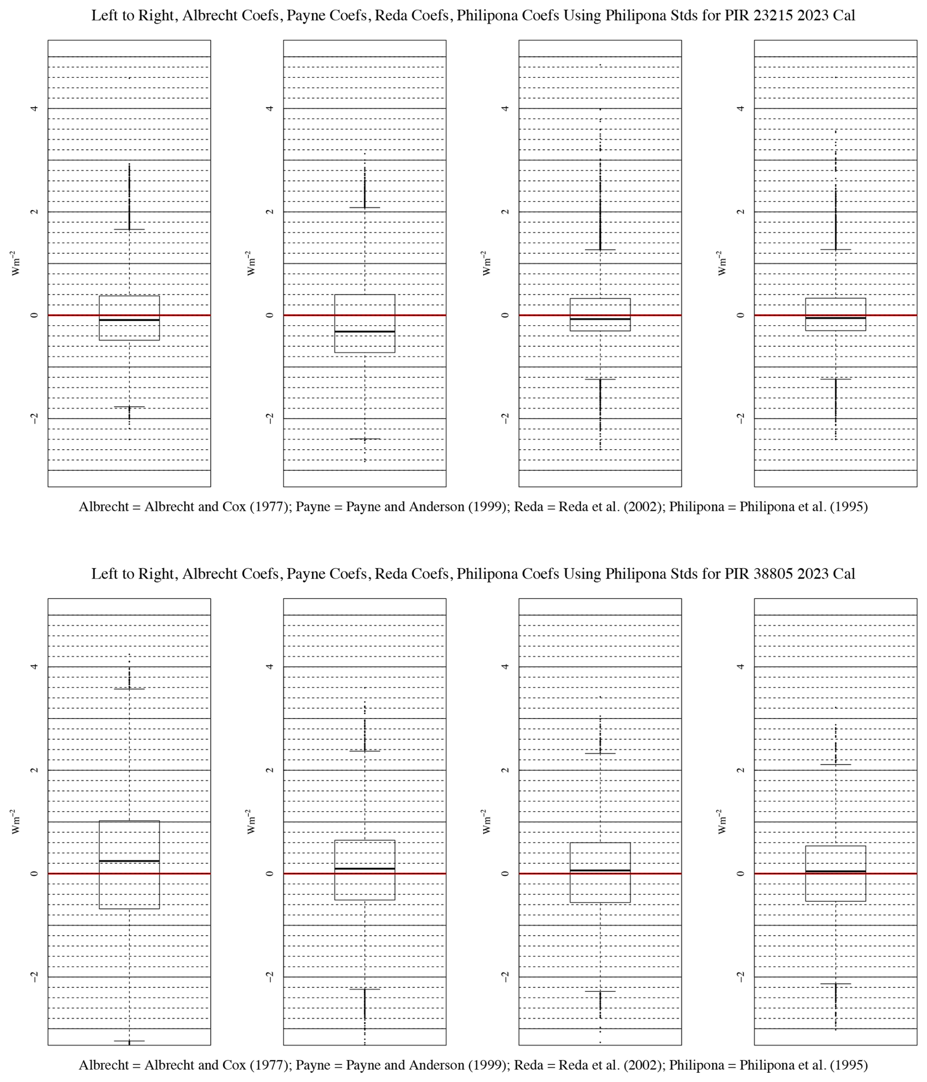
Figure 5 Boxplots of differences using the WRC's Philipona et al. (1995) coefficients for the standard PIRs and calibrated PIRs to this standard using the four equations to calculate incoming IR. Top is for PIR 23215 and bottom is PIR 38805 as in Fig. 4. Compare box widths, whisker lengths, and medians.

In these comparison plots the standard used was calibrated with Philipona et al. (1995) coefficients rather than Albrecht and Cox (1977) as in Fig. 4. Similar results were obtained for the other four PIRs with the best results always obtained with the Philipona et al. (1995) formulation. In only one case out of the six the Payne and Anderson (1999) formula performed slightly better than the Reda et al. (2002) formula (not shown).

T-tests were performed to assess differences when using non-Philipona et al. (1995) calibration coefficients for all six calibrated instruments. If one assumes that there are no significant differences in the calculation of IR irradiances using the Philipona et al. (1995) formula versus each of the other three methods discussed, this assumption is rejected with 95 % confidence in 15 of the 18 cases studied (six calibrated PIRs and three formulae). The three cases where the null hypothesis cannot be rejected with 95 % confidence are for three of the six PIRs using the Reda et al. (2002) formula.

Reda et al. (2002) and Payne and Anderson (1999) did not use the measured body temperature T_B in their formulae, but estimated the receiver temperature T_B using a form of Eq. (5) for their particular PIR configuration. As a test we replaced T_B with T_R in the Philipona et al. (1995) Eq. (3). The extremely small changes in the rightmost boxplots of Fig. 5 were imperceptible. We would, therefore, suggest keeping Eq. (3) in its original form for calibration transfer.

4 Precision of the PIR Standards

The calibration of our same three standard PIRs at the WRC leads to slightly different calibration results. Here, the consistency and repeatability of those calibration events is assessed. The PIRs that we use for standards were sent to WRC in 2018, 2022, and 2024. For each of those events, coefficients for the Albrecht and Cox (1977) and Philipona et al. (1995) forms of the PIR processing equation for calculating incoming IR were provided by the WRC.

Our calibration seasons typically run from Spring to early Fall. Therefore, our three standard PIRs experience roughly six months of exposure to the weather each year. In Fig. 6 differences from applying three sets of WRC Philipona calibration coefficients (from 2018, 2022, and 2024) to the same dataset (that used for Fig. 3) are summarized. For example, calibrations from 2018 and 2022 were applied to the same dataset and differences in irradiance for each minute were tallied and summarized in boxplots. Differences for all permutations are mostly within 1 W m⁻² and suggest that errors from applying one of the WRC calibrations from any of the three calibration years to any year would be less than the uncertainty of the WRC calibrations themselves (∼4 W m⁻²; https://www.pmodwrc.ch/en/?s=wisg, last access: 3 February 2026). This suggests that the Eppley PIR is very stable and should be suitable for monitoring long-term changes in the thermal IR.

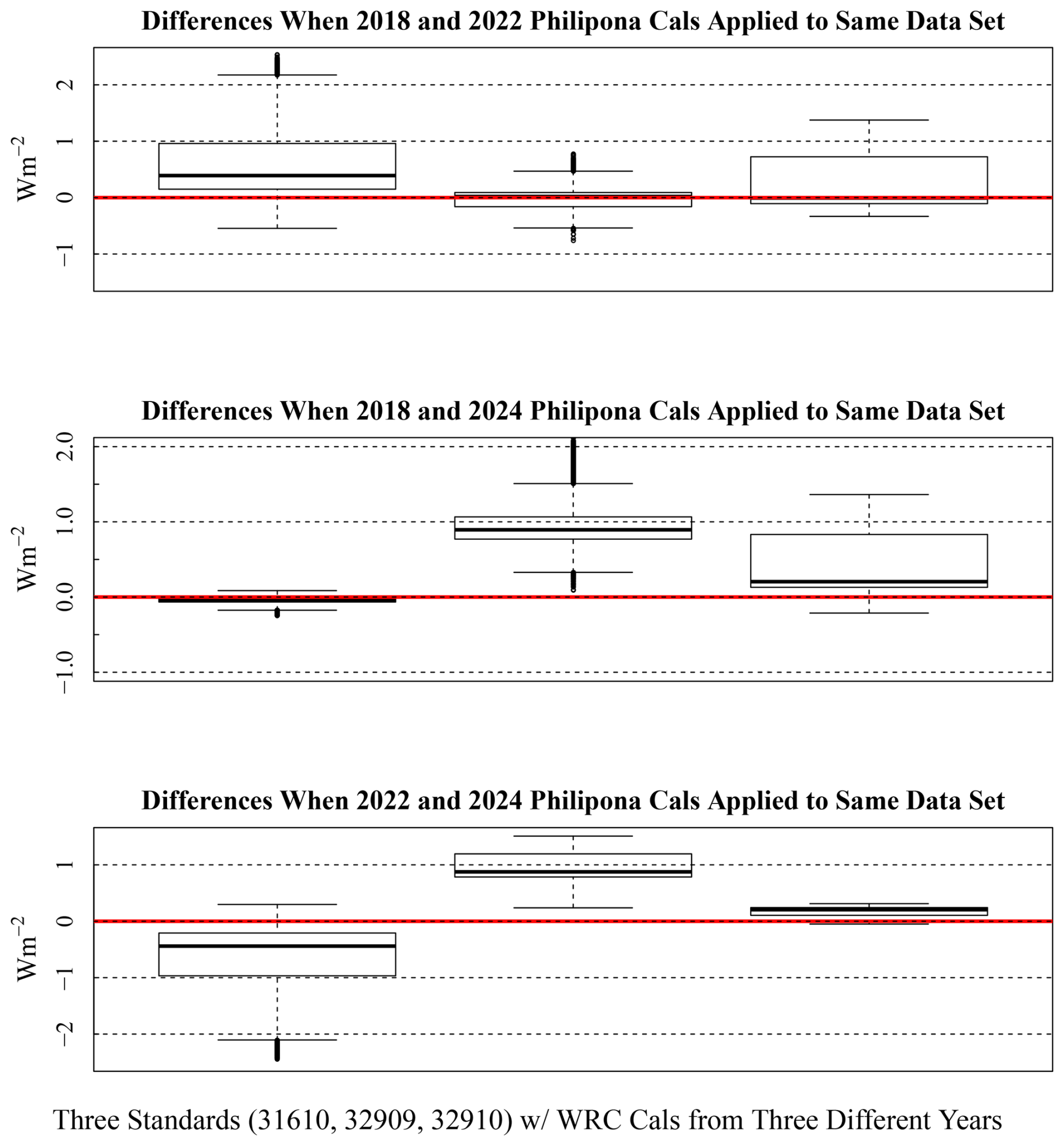
Figure 6 Comparisons of three sets of Philipona et al. (1995) calibration coefficients provided by the WRC in 2018, 2022, and 2024 applied to the same data set as in Fig. 3 for the three PIRs used as standard PIRs with serial numbers in the subtitle. The medians are all within 1 W m⁻² and most are within 0.5 W m⁻².

In Sect. 3 the average output of the three standard PIRs is used to derive new calibration coefficients for each test PIR. Using those new calibrations, the test instrument measurements are compared to the standard PIRs' average over the entire calibration period. For the left panels in Fig. 7 we use Philipona et al. (1995) coefficients for the standard PIRs to calibrate the three test PIRs (serial numbers shown at the top of each subplot). We apply those new calibrations and subtract the results from the standard PIRs' average for each minute and summarize the distribution of differences in boxplots. Therefore, the leftmost panels of Fig. 7 replicates the rightmost panels of Figs. 4 and 5. This is not an independent test of the reliability of the calibration because the same dataset is used for calibration and verification.

To test new calibrations with an independent dataset, the time series in Fig. 3 is divided in half. The middle panels of Fig. 7 use the first half of the data in Fig. 3 to derive a calibration and the second half of the data to validate the new calibration against the standard PIRs' average. Then, we reverse this process using the second half of the Fig. 3 data for calibrating and the first half to validate. If we examine the time series in Fig. 3, it is apparent that the first half of the data stream is noisier than the second half. Using the first half of the data to calibrate and applying to the second half and vice versa is likely responsible for the offsets in the medians, but the offsets are less than 1 W m⁻². Note that when the less noisy data of the second half are used to validate (middle boxplots) the differences have a smaller spread. When the noisier first half data (rightmost boxplots) are used to validate, the differences have a larger spread. Examining the top, middle, and bottom plots, there are differences inherent in the instruments themselves since boxplots are not replicated from PIR to PIR. Attribution to the instruments themselves is warranted because the standard PIRs and test data used for Fig. 7 were collected simultaneously.

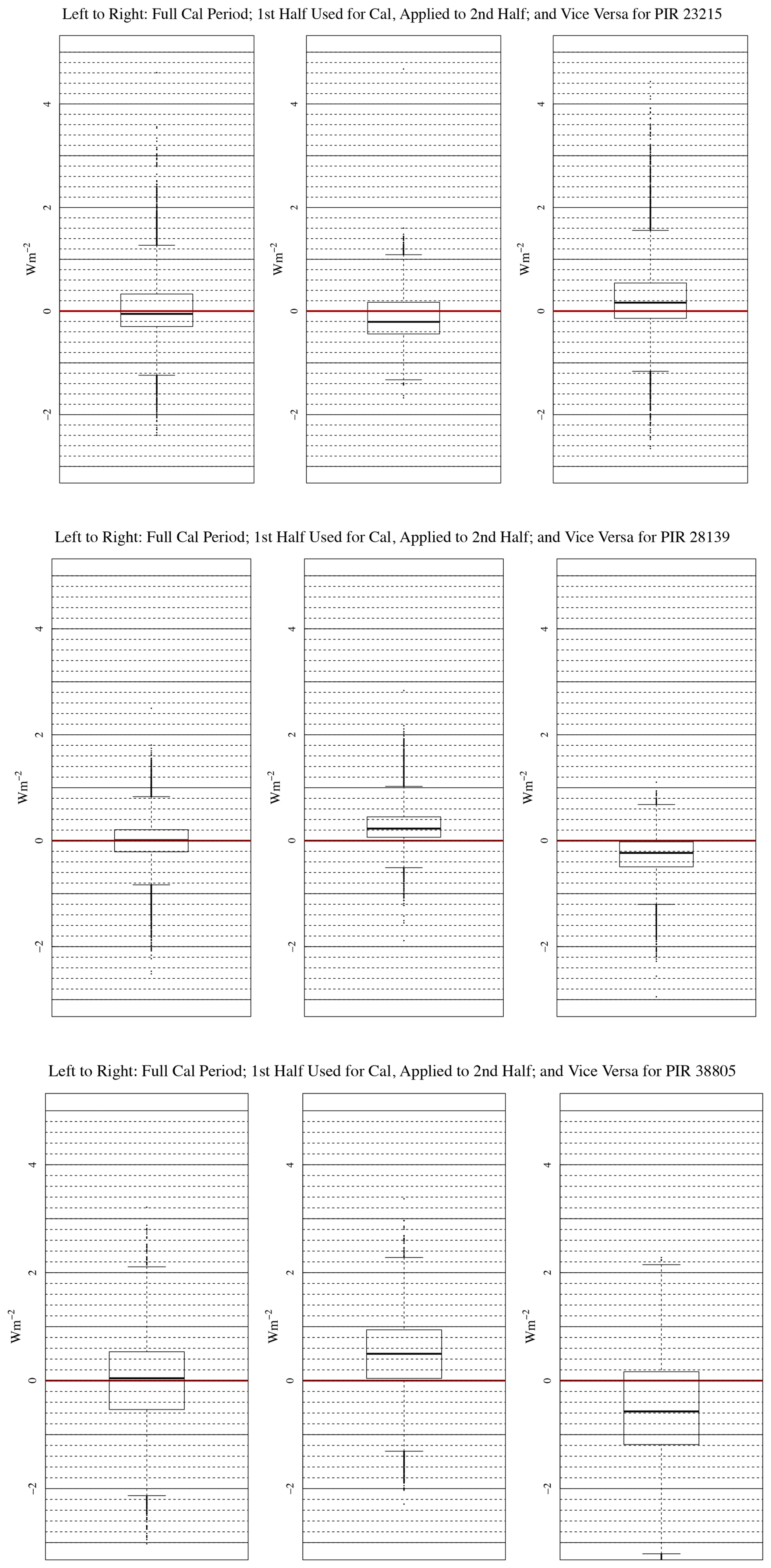
Figure 7 The leftmost panel uses the entire period in Fig. 3 to calibrate the named PIR and then compares the calibrated PIR data to the standard PIRs' average. The middle panel uses the first half of the period to calibrate and then assesses the application of those calibrations to an independent data set in the second half. The rightmost panel reverses this using the second half of the period for calibration and the first half for assessment.

5 Summary and Conclusions

In this paper we investigate four formulations for converting raw voltage and body and dome temperature measurements of an Eppley pyrgeometer, model PIR, to thermal IR irradiance. These methods are described in Albrecht and Cox (1977), Philipona et al. (1995), Reda et al. (2002) and Payne and Anderson (1999). All are slight variations of the original formulation of Albrecht and Cox (1977). Because the temperature measurements are critical to the infrared calculations, we also investigated various fits that have been applied to the Steinhart and Hart (1968) equation that converts thermistor-measured resistance to temperature.

Regarding the computation of thermistor temperatures, we found that fitting the manufacturer-supplied table of resistance and temperature (1 °C interval) to the range −50 to 50 °C provides the least variability as opposed to fits to shorter temperature ranges. However, differences of the fit to the provided data are <0.01 °C, regardless of the range used. Based on this result, we conclude that differences in thermistor temperature calculations from fits based on various temperature ranges do not have a significant impact on PIR measurements.

The three standard PIRs that we use to transfer calibrations from the world standard to field PIRs are calibrated frequently against the World Infrared Standard Group (WISG) at the World Radiation Center in Davos, Switzerland. They are returned with calibration coefficients for the Albrecht and Cox (1977) and Philipona (1995) methods, although the Albrecht and Cox coefficients provided are for the shortened form of their equation (Eq. 2). Comparing the application of the two methods to the standard PIRs revealed that the Philipona (1995) method is more precise and less noisy than the shortened Albrecht and Cox formulation; the differences are quantified in Fig. 3 (bottom) histograms. Comparisons were also made among three distinct WRC calibration results for the standard PIRs in 2018, 2022, and 2024. They showed that the three standard PIRs are stable, with the calibration coefficients changing minimally between WRC calibrations, and differences in irradiance calculations among applications of the separate biennial calibrations are within 1 W m⁻² of each other.

Application of the four methods for converting PIR raw measurements to irradiance was analyzed using six test instruments. The major conclusion is that use of the Philipona et al. (1995) form, i.e., Eq. (3), consistently does the best in transferring the mean calibration of the standard PIRs to field-deployed PIRs. Note that Reda et al. (2002) and Payne and Anderson (1999) coefficients are not available for the standard PIRs calibrated at the WRC, which may have led to some of the differences in Fig. 5. Of the six calibration comparisons, like those in Fig. 5, Reda et al. (2002) calibration results were close to, but statistically different than the Philipona et al. (1995) results on three of the six PIRs according to t-tests performed at the 95 % level. However, this agreement was found to be insignificant for the t-tests on the other three PIRs.

Given the differences in Figs. 6 and 7, it is probable that there is greater uncertainty caused by the particular atmospheric conditions under which calibrations are carried out. With the assumption that the PIR is very stable, the variations among the instruments in Fig. 6 could be subtle differences in atmospheric conditions during the three calibration sessions at the WRC in 2018, 2022, and 2024. This is reinforced by the differences in Fig. 7, where independent stable (i.e., clear), and unstable (e.g., intermittent clouds) periods were used to calibrate test instruments, with differing results. Note that PIR measurements for any arbitrary weather condition are often going to have larger uncertainties than discussed here.

The WISG, which is used for calibration at the WRC, is the current standard for broadband IR measurements. It has an uncertainty of 2.6 W m⁻². Recent studies, which are summarized in Gröbner et al. (2024), further suggest that the current WISG may be low by as much as 4 W m⁻² if the water vapor column exceeds 1 cm, but the difference is smaller if the atmosphere is dryer approaching no difference for vanishing water vapor (see Fig. 2 in Gröbner et al., 2024). Nevertheless, a new standard for broadband IR radiation is not expected to be established until the next WMO congress in 2027 at the very earliest (Laurent Vuilleumier, personal communication, 16 April 2025).

Appendix A: Differences fitting ohms vs kiloohms in Eq. (7) if no quadratic term

Fitting the manufacturer-supplied temperature (at 1 °C intervals) and resistance data, separately in ohms and in kiloohms, led to an unexpected outcome. First, if a full cubic (i.e., non-zero coefficient for the squared term) least-squares fit of the Steinhart-Hart equation with YSI 44031 data in kiloohms is compared to a least-squares fit using ohms, identical fits are obtained (blue and white dashed line in Fig. 2). If the quadratic term is set to zero and the fits are made to ohms and then kiloohms, we see a significant difference as shown in Fig. A1. This difference is due to numerical reasons, which are explained in the following.

First, it must be noted that the lack of significant digits when using kiloohms is not an issue because for the fits here, kiloohms are computed simply by dividing the resistance value in ohms by 1000, keeping significant digits in the decimal places.

The requirement of a quadratic term for expressing the Steinhart-Hart equation in kiloohms can be demonstrated by substituting for R in Eq. (7) 1000R_k, where R_k is in units of kiloohms as shown in Eq. (A1).

$$\begin{array}{}\text{(A1)}& \mathrm{1}/T=a+b\cdot \ln \left(\mathrm{1000}{R}_k\right)+d\cdot \ln {\left(\mathrm{1000}{R}_k\right)}^{\mathrm{3}}\end{array}$$

Applying logarithm rules to Eq. (A1) results in Eq. (A2).

$$\begin{array}{}\text{(A2)}& \begin{array}{rl}\mathrm{1}/T& =a+b\left(\ln \left(\mathrm{1000}\right)+\ln \left(R_k\right)\right)+d\left(\ln \left(\mathrm{1000}\right)\right.\\ & {\left.+\ln \left(R_k\right)\right)}^{\mathrm{3}}\end{array}\end{array}$$

Expanding and regrouping terms in Eq. (A2) then gives Eq. (A3) through Eq. (A7).

$$\begin{array}{}\text{(A3)}& {\displaystyle }\mathrm{1}/T=a_k+b_k\cdot \ln \left(R_k\right)+c_k\cdot \ln {\left(R_k\right)}^{\mathrm{2}}+d_k\cdot \ln {\left(R_k\right)}^{\mathrm{3}}\text{(A4)}& {\displaystyle }{a}_k=a+b\cdot \ln \left(\mathrm{1000}\right)+d\cdot \ln {\left(\mathrm{1000}\right)}^{\mathrm{3}}\text{(A5)}& {\displaystyle }{b}_k=b+\mathrm{3}d\cdot \ln {\left(\mathrm{1000}\right)}^{\mathrm{2}}\text{(A6)}& {\displaystyle }{c}_k=\mathrm{3}d\cdot \ln \left(\mathrm{1000}\right)\text{(A7)}& {\displaystyle }{d}_k=d\end{array}$$

Thus, when data are in kiloohms an equation of the form of Eq. (A3) (i.e. full cubic) is required to match the results of Eq. (7) when data are in units of ohms. Thus, changing units of R in Eq. (7) results in a full cubic equation. This implies that a full cubic equation can be more robust than Eq. (7) when fitting data where units other than ohms are used for R. It also demonstrates that it is possible to change units for R in Eq. (7) analytically using the substitution process shown above rather than refitting if desired.

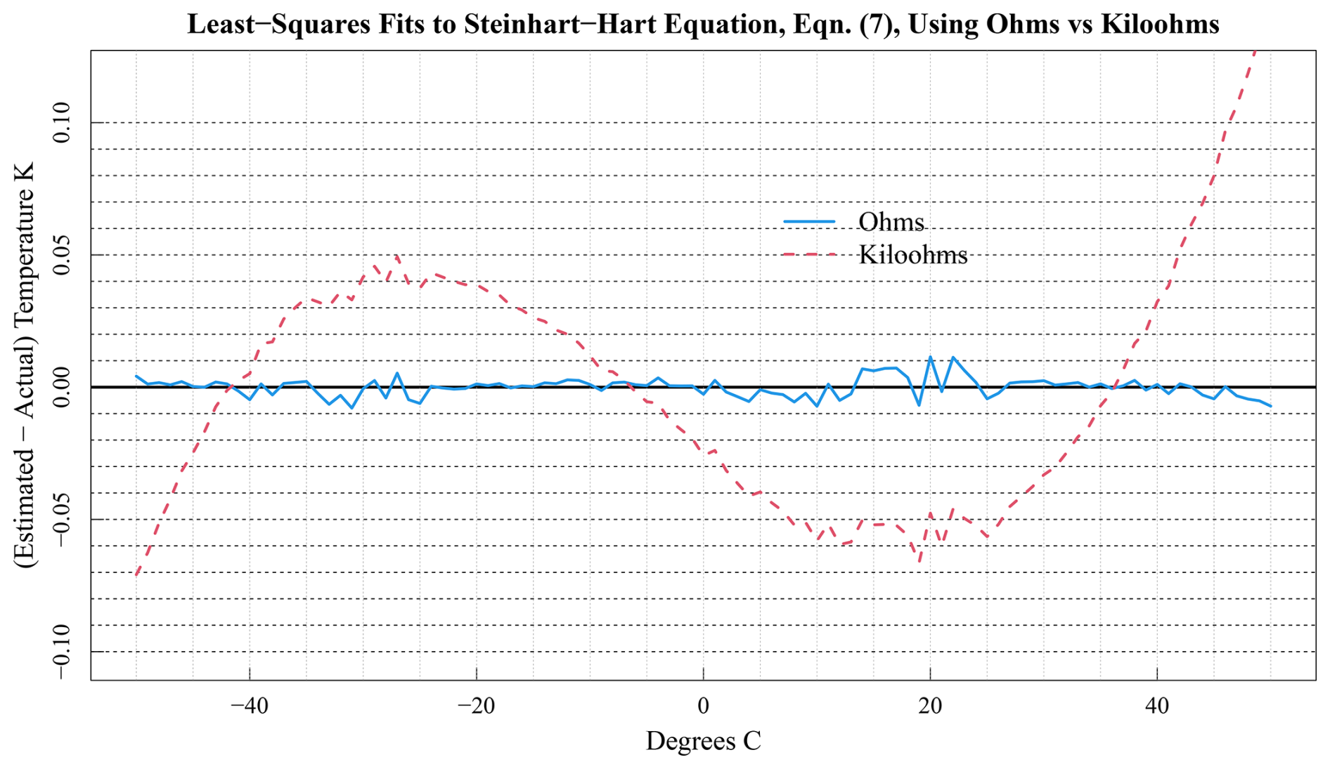
Figure A1 Steinhart-Hart equation (i.e., no quadratic term) fit to ohms (blue solid line) versus kiloohms (red dashed line).