Solar Backscatter Ultraviolet (BUV) retrievals of mid-stratospheric aerosols from the 2022 Hunga Eruption

On 15 January 2022, a highly explosive eruption of the submarine Hunga volcano (Kingdom of Tonga) generated the largest stratospheric hydration event ever observed and the largest aerosol perturbation since the 1991 Pinatubo eruption. Here, we develop a novel method for satellite retrieval of stratospheric aerosol optical depth (AOD) and layer peak height (z_p) using solar backscattered ultraviolet (BUV) radiation; this is made possible by the exceptional mid-stratospheric altitude of the Hunga aerosols. We analyze BUV observations of the Hunga stratospheric aerosol cloud on 17 January 2022 (47 h after the eruption), using BUV band 1 measurements from the TROPOspheric Monitoring Instrument (TROPOMI) on board the ESA/Copernicus Sentinel-5 precursor (S5P) satellite, and the Ozone Mapping and Profiling Suite- Nadir Profiler (OMPS-NP) on board the National Oceanic and Atmospheric Administration (NOAA)-20 satellite. We retrieve AOD and z_p by fitting hyperspectral BUV radiance ratios in a narrow spectral window restricted to 289–296 nm, chosen in order to reduce interference from tropospheric clouds while highly sensitive to stratospheric aerosols located above ozone peak altitude. The retrieval employs radiative transfer calculations from the Vector Linearized Discrete Ordinate Radiative Transfer (VLIDORT) forward model. We assume a single Hunga aerosol layer composed of polydisperse sulfuric acid spherical particles embedded in a Rayleigh atmosphere with a known ozone profile. The ozone profile is supplied from a version of the Modern-Era Retrospective analysis for Research and Applications, version 2 (MERRA-2) Stratospheric Composition Reanalysis of the Microwave Limb Sounder (MLS) on board NASA Earth Observing System-chemistry (EOS Aura) satellite – produced by NASA's Global Modeling and Assimilation Office using a stratospheric chemistry model and MERRA-2 meteorology. We also include a sulfur dioxide SO₂ layer, which coincides spatially with the retrieved aerosol vertical profile, and with the total loading normalized to the stratospheric SO₂ vertical column density from the operational TROPOMI SO₂ product. We validate our AOD retrievals against ground-based AErosol RObotic NETwork (AERONET) direct-sun AOD measurements, and z_p retrievals against Cloud-Aerosol Lidar with Orthogonal Polarization (CALIOP) overpasses using Lagrangian trajectory modeling. We estimate the total Hunga stratospheric wet aerosol mass (sulfuric acid solution droplets, including water uptake) to be $M_{\mathrm{aer}}\sim \mathrm{0.5}\pm \mathrm{0.05}$ Tg. This value is consistent with our previous BUV estimates of Hunga SO₂ emissions (∼ 0.4–0.5 Tg SO₂) and rapid conversion of SO₂ to sulfate aerosol. Based on these BUV retrievals we can also estimate the sulfuric acid (H₂SO₄) mass fraction w∼0.4 and ${\mathrm{H}}_{\mathrm{2}}{\mathrm{SO}}_{\mathrm{4}}/{\mathrm{H}}_{\mathrm{2}}\mathrm{O}$ solution density: ρ∼1.34 g cm⁻³. These new values represent an extreme departure from the stratospheric background sulfate aerosol (Junge layer), which is typified by values of w∼0.75 and ρ∼1.7 g cm⁻³ supported by decades of observations of the lower stratosphere during both quiescent and volcanically impacted periods. The new low values, inferred from BUV observations and backed up by microphysical modeling, are a result of the uniquely water-rich conditions in the early Hunga plume. Relative humidity in the plume, as modeled by the NASA Goddard Earth Observing System Chemistry-Climate Model with the Community Aerosol and Radiation Model for Atmospheres (CARMA), reached values as high as 60 %, compared to background values closer to 1 %. These findings are unique in the long-term observational record of the stratosphere; similar relative humidities only otherwise occur in overshooting clouds or cold winter hemisphere vortices.

1 Introduction

A paroxysmal eruption of the submarine Hunga volcano (Kingdom of Tonga; 20.550° S, 175.385° W) at ∼ 04:15 UTC on 15 January 2022 produced a steam-driven eruption column up to ∼ 58 km altitude (APARC, 2025; Carr et al., 2022; Millán et al., 2022) and injected a massive plume of water vapor (H₂O), sulfur dioxide (SO₂), and aerosols directly into the Southern tropical stratosphere (Carn et al., 2022; Coy et al., 2022; Khaykin et al., 2022; Millán et al., 2022; Legras et al., 2022; Schoeberl et al., 2023; Sellitto et al., 2022; Taha et al., 2022; Vömel et al., 2022). This was the largest volcanic explosion observed from space since Pinatubo in 1991, with a designated Volcanic Explosivity Index (VEI) of 5–6 (APARC, 2025). The Hunga eruption produced enormous umbrella cloud(s) with diameter(s) > 500 km, global Lamb waves (Kubota et al., 2022; Matoza et al., 2022), regional volcanic ash fall (Kelly et al., 2024), and Pacific-wide tsunamis (Lynett et al., 2022; Shrivastava et al., 2023).

Although volcanic ash ejecta remained at relatively low altitudes and quickly fell out over the Tonga area (Kelly et al., 2024), sub-micron non-absorbing, non-depolarizing sulfuric acid (sulfate)-type aerosol particles persisted in the mid-stratosphere (Khaykin et al., 2022; Sellitto et al., 2022; Taha et al., 2022; Baron et al., 2023; Bernath et al., 2023; Bian et al., 2023; Boichu et al., 2023; Bourassa et al., 2023; Duchamp et al., 2023; Manney et al., 2023; Kahn et al., 2024; Stocker et al., 2024; Sicard et al., 2025). Discussions on the H₂O-accelerated conversion of volcanic SO₂ to sulfate aerosol may be found in previous studies (Carn et al., 2022; Legras et al., 2022; Sellitto et al., 2022, 2024; Zhu et al., 2022; Asher et al., 2023, Boichu et al., 2023; Bruckert et al., 2025; Sadeghi et al., 2025; Stenchikov et al., 2025) summarized in the Hunga volcanic eruption atmospheric impacts report (APARC, 2025).

Initial estimates of the Hunga SO₂ emissions from solar backscatter ultraviolet (BUV) near-nadir satellite measurements did not account for interference from stratospheric aerosols; indeed, unexpectedly low amounts were reported for an eruption of this magnitude: ∼ 0.4–0.5 Tg SO₂ (Carn et al., 2022). Infrared (IR) satellite measurements from the Cross-track Infrared Sounder (CrIS) instrument (Hyman and Pavolonis, 2020) retrieved a similar amount: ∼ 0.4 Tg SO₂ (Sadeghi et al., 2025); however, retrievals from the Infrared Atmospheric Sounding Interferometer (IASI) reported roughly double this amount, i.e., >1 Tg SO₂ (Sellitto et al., 2022, 2024; Bruckert et al., 2025). These conflicting estimates provide a strong motivation to re-analyze BUV SO₂ measurements with explicit consideration of Hunga aerosol interference. To do this, we need first to introduce a suitable Hunga aerosol optical model in the UV and then develop a new quantitative BUV retrieval of non-absorbing stratospheric aerosol particles. Such nadir-BUV aerosol retrievals were not thought to be possible prior to the Hunga event; indeed, this is the first eruption in the modern satellite era to inject particles directly into the mid-stratosphere above the tropical ozone (O₃) density peak at ∼ 25 km (Carr et al., 2022; Taha et al., 2022). This unique geophysical event provides access to solar backscattered shortwave UVB radiation (<300 nm wavelength) that is strongly absorbed by ozone before reaching the lower stratospheric altitudes typical of volcanic aerosol injections. Another motivation for the present study is that during the early dispersion phase, the presence of Hunga aerosols significantly affected the BUV satellite retrievals of stratospheric ozone (Bhartia et al., 1993; Torres and Bhartia, 1995; Kramarova, 2024), as well as ocean color retrievals (Franz et al., 2024).

Figure 1 shows a Visible Infrared Imaging Radiometer Suite (VIIRS) true color map from 17 January 2022, two days after the main Hunga eruption. The approximate locations of two distinct Hunga plumes are outlined over the Queensland region of Australia (aerosol-rich plume; C1) and over the Coral Sea (SO₂–rich plume; C2) – see Fig. 5d in Carn et al. (2022) and Fig. 4b–d in Legras et al. (2022). These two plumes showed different altitudes and compositions and evolved differently during the first weeks after the eruption before eventually mixing. The aerosol-rich C1 plume was also water-rich, which likely accelerated the SO₂-to-sulfate conversion and enhanced radiative cooling, thus contributing to its more rapid descent compared to that of the SO₂-rich C2 plume. Also indicated in Fig. 1 are the overpass times of key satellite tracks: the National Oceanic and Atmospheric Administration (NOAA)-20 Ozone Mapping and Profiler Suite (OMPS) Nadir Profiler (NP) swath (∼ 04:00–04:09 UTC), the Cloud-Aerosol Lidar with Orthogonal Polarization (CALIOP) daytime track (∼ 05:23–05:34 UTC), and nighttime tracks (∼ 16:14–16:25 UTC and ∼ 17:54–18:05 UTC). These times indicate that the observations were not simultaneous, but together they provide a complementary view of the rapidly evolving plume (≈20° longitude per day; see also Fig. 7). The OMPS nadir profiler sensor (OMPS-NP), which has a spatial resolution of 50 km at nadir, is designed to measure stratospheric ozone profiles using BUV wavelengths above and below 300 nm, but as a nadir-sounding sensor it does not provide adequate horizontal coverage of the Hunga aerosol plume. Nevertheless, the well-placed OMPS-NP overpass of the Hunga plume on 17 January (Fig. 1) did provide the first spectral observations of significantly enhanced BUV radiances produced by the Hunga aerosols at wavelengths around 300 nm.

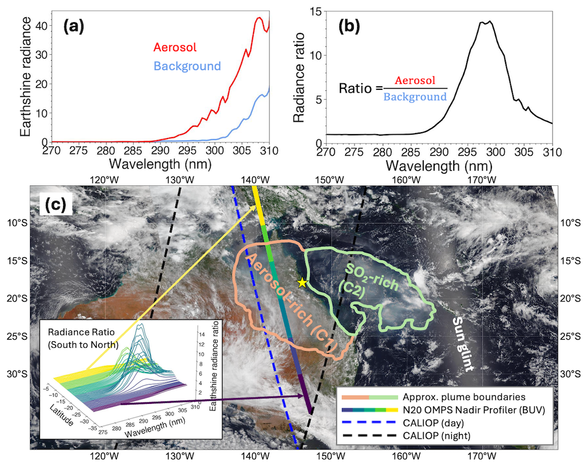
Figure 1 (a) Shortwave BUV radiances (270–310 nm) of aerosol-rich and background (aerosol-free) regions. (b) Spectral radiance ratios (aerosol/background). (c) True-color NOAA-20 VIIRS map of Australia and the Coral Sea on 17 January 2022. The solid line with colored segments shows the suborbital track of the NOAA-20 OMPS-NP (∼ 04:00–04:09 UTC). The inset panel at bottom left shows the variation of spectral radiance ratio with latitude measured by OMPS-NP in the Hunga aerosol plume. Dashed lines are CALIOP ground tracks – blue for daytime (∼ 05:21–05:32 UTC) and black for nighttime (left: ∼ 17:54–18:05 UTC, right: ∼  16:14–16:25 UTC). The yellow star indicates the location of the Aerosol Robotic Network (AERONET) Lucinda site (18.5198° S; 146.3861° E; elevation: 8.0 m).

Accordingly, to estimate Hunga aerosol optical depth (AOD), layer peak height (z_p), and column mass, we have analyzed BUV observations taken by an imaging spectrometer – TROPOspheric Monitoring Instrument (TROPOMI) on board the Copernicus Sentinel-5 precursor (S5P) satellite. TROPOMI is eminently suitable for this task, because of its contiguous daily coverage and high spatial resolution (nominally 5.5 km by 28 km below 300 nm in band 1) (Veefkind et al., 2012; Ludewig et al., 2020). On 17 January at ∼ 03:16 UTC (47 h after the 15 January eruption) the bulk of the Hunga aerosol was observed over Northeast Australia (Fig. 1), while the bulk of the attendant SO₂ plume was trailing over the Coral Sea (see also Fig. 5d of Carn et al., 2022).

We use such BUV spectral enhancements to develop a new algorithm for retrievals of non-absorbing aerosol optical depth (AOD) and peak-height (z_p) as well as estimates of column wet aerosol mass (i.e., sulfuric acid solution droplets, ${\mathrm{H}}_{\mathrm{2}}{\mathrm{SO}}_{\mathrm{4}}/{\mathrm{H}}_{\mathrm{2}}\mathrm{O}$ including water uptake), m_aer, sulfate (H₂SO₄) mass fraction, w, and solution density, ρ. The retrieval algorithm is based on spectral fitting of hyperspectral BUV radiance ratios with the forward model driven by the Vector Linearized Discrete Ordinate Radiative Transfer (VLIDORT) model (Spurr and Christi, 2019) and combined with polydisperse Mie calculations of aerosol optical properties (i.e., spectral extinction and scattering matrices). Based on collocated Cloud-Aerosol Lidar with Orthogonal Polarization (CALIOP) backscatter measurements (Fig. 7), we have assumed a single aerosol layer composed of spherical polydisperse homogeneous ${\mathrm{H}}_{\mathrm{2}}{\mathrm{SO}}_{\mathrm{4}}/{\mathrm{H}}_{\mathrm{2}}\mathrm{O}$ solution particles embedded in a Rayleigh-scattering atmosphere with known ozone and temperature profiles. We also included the SO₂ vertical profile, assumed spatially coincident with the retrieved aerosol plume, but normalized to the TROPOMI operational stratospheric SO₂ column density (Theys et al., 2017).

This paper begins by summarizing the TROPOMI UV band 1 (UV1) measurements (Sect. 2). Section 3 describes our retrieval algorithm, comprising an overview of the retrieval strategy (Sect. 3.1), deployment of the VLIDORT-based forward model component (Sect. 3.2), the inverse model (Sect. 3.3), a discussion on aerosol optical properties and trace gas parameterization (Sect. 3.4), and a validation of the retrieval algorithm using synthetic data (Sect. 3.5). In Sect. 4, we present our results on the retrieval and validation of aerosol peak height (Sect. 4.1) and AOD (Sect. 4.2), followed by estimates of the column wet aerosol mass, m_aer and total aerosol mass including water uptake, M_aer (Sect. 4.3). In addition, we estimate H₂SO₄ (sulfate) mass fraction, w and ${\mathrm{H}}_{\mathrm{2}}{\mathrm{SO}}_{\mathrm{4}}/{\mathrm{H}}_{\mathrm{2}}\mathrm{O}$ particle mass density, ρ (Sect. 4.4). Section 4.5 contains comparisons with recent IR-based retrievals of SO₂ and Hunga aerosol mass from other studies of this unique event. Section 5 concludes with a summary of the paper along with final remarks.

2 Solar backscatter measurements in the UV (BUV)

This section describes measurement data. First, we focus on the TROPOMI band 1 backscatter measurements used for the aerosol plume retrieval; this is followed by a discussion on anomalies in the satellite BUV ozone record caused by the Hunga eruption.

2.1 TROPOMI band 1 radiances and radiance ratios

A detailed description of the current version of the TROPOMI Level 1B radiance product (L1B_RA_BD1), including the data file format in NETCDF-4 and the data fields, is given in the TROPOMI Level 1B product “readme” file (https://doi.org/10.5270/S5P-kb39wni, Ludewig, 2023). TROPOMI provides excellent spatial resolution and daily global coverage in the shortwave BUV band 1 (267–300 nm); however, TROPOMI has known radiometric and sensor degradation issues in band 1 (Ludewig et al., 2020), and it has been proved necessary to apply soft calibration techniques to improve the data quality. The TROPOMI soft calibration is computed from characterization of the differences between measured and modelled radiances (absolute residuals), following a similar approach to that described in Mettig et al. (2021). Since this soft calibration is designed to correct input radiances for the TROPOMI ozone profile data product, forward Radiative Transfer (RT) model calculations were performed over the combined spectral range of band 1 and 2 (270–330 nm). Pressure, temperature, and ozone profiles from the Copernicus Atmosphere Monitoring Service (CAMS) were used as inputs to the RT model. Additionally, CAMS ozone profiles were scaled to match total ozone columns derived from the independent OMPS Nadir Mapper gridded column ozone data (Jaross, 2017). The modelled atmosphere does not contain clouds nor aerosols, but particulate scattering effects are compensated through adjustment of the surface albedo. With this in mind, we have fitted the scene albedo in a small spectral window (328–330 nm) and assumed this albedo to be representative for the entire fitting window. Radiance residuals (measurement to model) are computed for single seasonal TROPOMI orbits over the Pacific Ocean. To compute correction parameters, the radiance residuals are compiled separately for each year and then applied to the radiance measurement in that year. Correction parameters are provided as a function of the TROPOMI cross-track position (i.e., CCD detector row number), wavelength and radiance level; they are applied to the uncorrected radiance signal (R_uncorr) by subtracting the bias (R_corr=R_uncorr-bias). For TROPOMI orbits 22086 and 22087 affected by Hunga aerosols on 17 January 2022 we apply the fixed correction available for the highest radiance.

One option for constructing the retrieval measurement vector is to use sun-normalized radiances, or the “N-values” (defined as N(λ) = $-\mathrm{100}{\log }_{\mathrm{10}}\left(\frac{R\left(\mathit{\lambda }\right)}{F\left(\mathit{\lambda }\right)}\right)$ where R denotes BUV absolute radiance and F incoming solar irradiance), as shown in Fig. 2 for two TROPOMI orbits (22086 and 22087) overpassing Hunga aerosol plume on 17 January 2022 (eastern orbit 22086 and the following orbit 22087) at four wavelengths, representative of the selected spectral fitting window: λ=287.9, 292.5, 295.1, 297.9 nm.

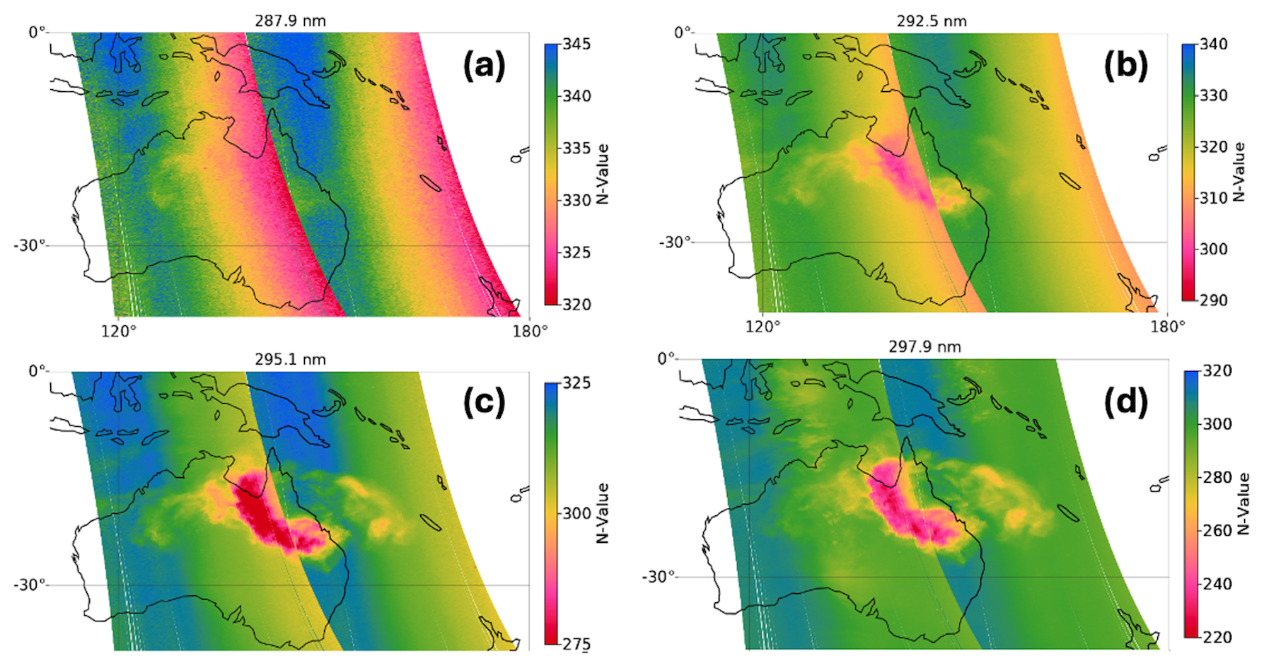
Figure 2 Maps of the Hunga aerosol plume on 17 January 2022, using TROPOMI band 1 sun-normalized radiances before applying soft-calibration at four wavelengths at (a) 287.9 nm, (b) 292.5 nm, (c) 295.1 nm, and (d) 297.9 nm in orbits 22086 (right-hand swath) and 22087 (left-hand swath). Plotted are the N-values, defined as $N\left(\mathit{\lambda }\right)=-\mathrm{100}{\log }_{\mathrm{10}}\left(\frac{R\left(\mathit{\lambda }\right)}{F\left(\mathit{\lambda }\right)}\right)$, where R(λ) denotes BUV radiance, and F(λ) the incoming solar irradiance. Note the different N-value scales for different wavelengths.

However, in order to emphasize the Hunga aerosol spectral signal and to reduce its dependence on TROPOMI band 1 calibration and degradation issues, we prefer to use BUV radiance ratios, in which the radiance values from the orbit 22086 and 22087 pixels are normalized to background radiances for the same cross-track pixels from an adjacent Hunga aerosol-free orbit, in this case TROPOMI background orbit 22085. These radiance ratios are plotted in Fig. 3. The advantage of normalizing to background radiances is that this pixel-wise division leads to a partial cancellation of known radiometric and degradation interferences from the TROPOMI band 1, as reported in Ludewig et al. (2020) and reduces sensitivity to ozone absorption. We do account for the ozone profile differences between the background (o22085) and Hunga (o22086 and o22087) orbits using modified MERRA-2 Stratospheric Composition Reanalysis of the Microwave Limb Sounder (MLS) on board NASA EOS Aura satellite as described later in Sect. 2.2. The normalization requires correction for tropospheric clouds if one uses longer band 2 wavelengths (see example for background pixel 1 in Fig. 3). Therefore, in this study we only use a short spectral fitting window from 289 to 296 nm which is not affected by tropospheric clouds.

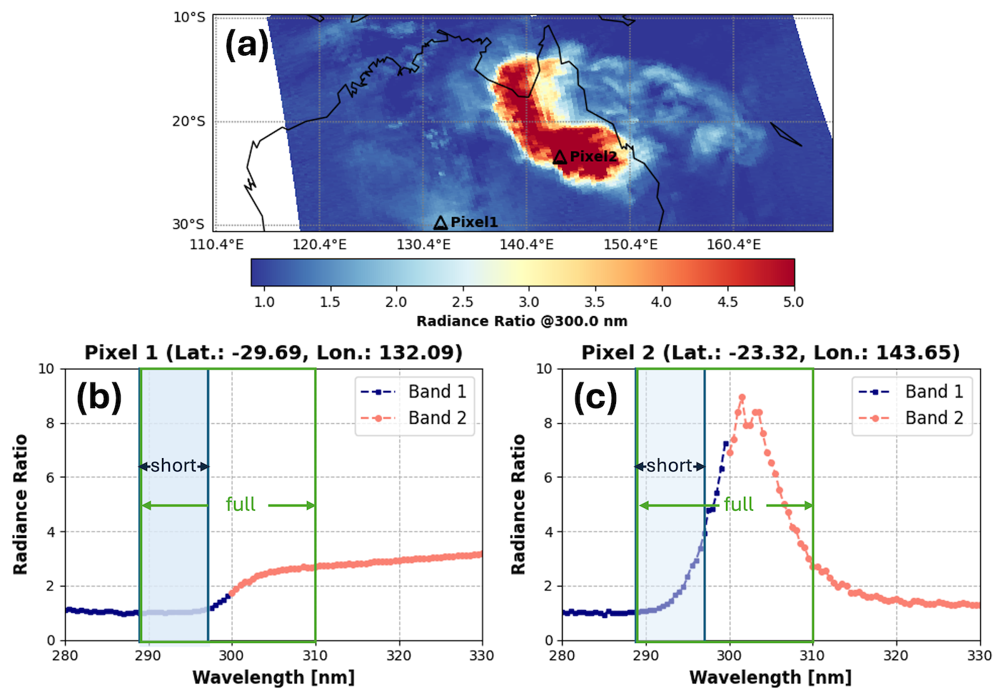
Figure 3 (a) Map of normalized TROPOMI radiance at 300 nm on 17 January 2022. Normalized TROPOMI radiance spectra for (b) a background (Hunga aerosol-free) pixel 1 and (c) a pixel 2 in the Hunga aerosol plume. The spectral radiance ratio plots indicate the coverage of TROPOMI UV bands 1 and 2 (with an overlap around 300 nm), as well as the “short” and “full” spectral fitting windows (only the short window is used for aerosol retrievals). Pixel 2 shows the typical enhancement of the radiance-ratio signal in the presence of Hunga aerosols, whereas pixel 1 shows the effect of tropospheric clouds, but only at longer wavelengths (>297 nm). Note that tropospheric clouds do not affect short UV wavelengths <296 nm, e.g., pixel 1 (b). We note that the separation between bands 1 and 2 occurs around 300 nm, but it also depends on the across-track location.

For the 2-parameter (AOD and aerosol peak height, z_p) aerosol retrievals in Sect. 4, we restrict the spectral fitting window from 289 to 296 nm (hereafter, denoted as the “short” window) to reduce interference from bright tropospheric clouds. Figure 3 shows radiance ratios (using TROPOMI orbit 22085 as background) over a large part of Australia, with six- to ten-fold enhancements of the radiance-ratio signal in the presence of stratospheric aerosol. Background pixel ratios show signals from tropospheric clouds, but ratios in the short wavelength window are free of such signals (Fig. 3; this is also seen in Fig. 2d, where cloud signals at wavelength 297.9 nm are apparent in the Australian Bight near the south-central coast).

Figure 4 presents spectral radiance ratio measurements at four selected wavelengths. At wavelengths shorter than 288 nm there is no Hunga aerosol signature because of strong absorption by ozone above the Hunga plume altitude. The major plume signature over Northeast Australia becomes much clearer for the longer wavelengths, 296 to 298 nm, but even at 292 nm (top right) there is evidence of a forward plume streamer at high altitude over Northwest Australia. Also of interest are the tropospheric cloud echoes near the south-central Australian coast, evident at the two longer wavelengths (lower plots), but not present at shorter wavelengths. This indication has allowed us to set a cloud screening spectral threshold at λ=296 nm. In Sect. S1 in the Supplement, we present an animated video of the full spectral scan of TROPOMI band 1 and band 2 combined radiance ratios from 280 to 330 nm in steps of 0.5 nm (https://doi.org/10.5446/70186, Choi, 2022).

We contour the Hunga stratospheric aerosol plume using a Cloud Screening Index (CSI), which is defined as a radiance ratio at 296 nm (see Appendix C for the CSI determination). Hereafter, we only consider TROPOMI pixels with CSI > 1.1 for Hunga aerosol retrievals.

Note that we have also considered 3-parameter retrievals, with the third state vector element being the total column SO₂ emitted simultaneously in the Hunga eruption; for this retrieval, we use the larger spectral fitting window (289–310 nm), denoted as the “full” window in Fig. 3. This retrieval takes advantage of strong SO₂ absorption features present in TROPOMI band 2 radiances (306–310 nm) but it does require the application of a cloud-correction step. This retrieval is currently under investigation.

2.2 Ozone anomalies

As noted in the Introduction, we are motivated here to discuss the disruption in the BUV stratospheric ozone record due to the Hunga aerosols. Anomalies in a number of total ozone column (TOC) products were observed in the presence of the Hunga eruption plume; notably, enhanced BUV scattering signals due to high-altitude aerosol from the Hunga plume were mistakenly interpreted as TOC depletion in BUV ozone retrievals from all instruments (OMI, OMPS, GOME-2, as well as TROPOMI). Mid-stratospheric aerosols are not represented in the forward models used for the operational TOC retrievals, resulting in artificial TOC depletion during episodes of elevated volcanic aerosol loading. In this regard, it was necessary to re-analyze raw BUV spectra to flag pixels affected by the Hunga aerosols. Indeed, the presence of such “bad-quality” ozone data will contaminate assimilation products that rely on BUV TOC data. For instance, artificially low BUV TOC data affected by Hunga plume resulted in anomalous assimilation outcomes in released M2-SCREAM reanalysis data (MERRA-2 Stratospheric Composition Reanalysis of Aura Microwave Limb Sounder (MLS) produced by NASA's Global Modelling and Assimilation Office using a stratospheric chemistry model and MERRA-2 meteorology (Gelaro et al., 2017; Wargan et al., 2023)), as shown in Fig. 5a.

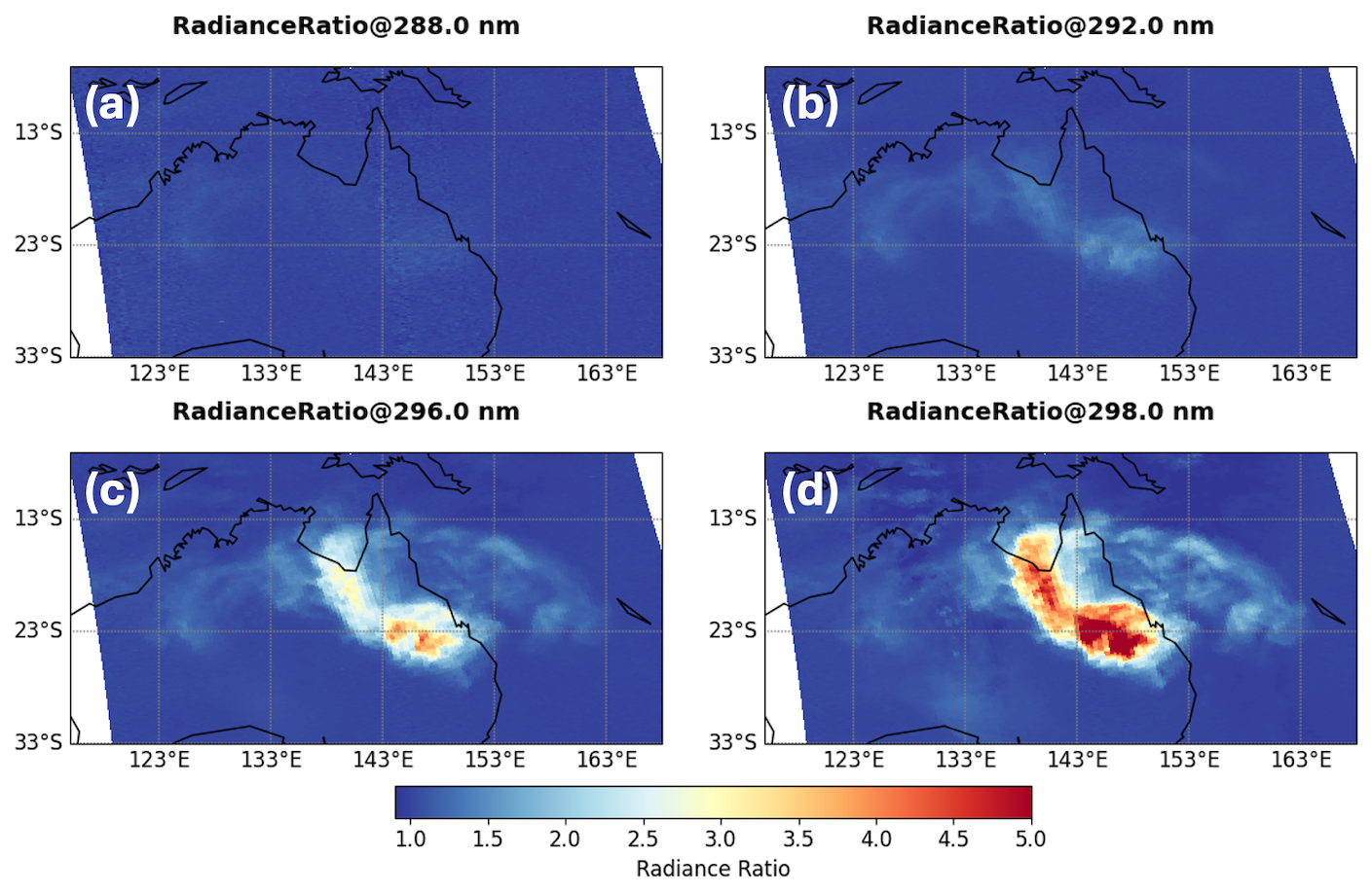
Figure 4 TROPOMI measured band 1 spectral radiance ratios (orbits 22086/22085 and 22087/22085) at (a) 288 nm, (b) 292 nm, (c) 296 nm, and (d) 298 nm. See the full spectral movie in Video Supplement S1 (https://doi.org/10.5446/70186, Choi, 2025).

In contrast, ozone profile measurements from MLS on board NASA Earth Observing System -chemistry (EOS Aura) satellite were not affected by the Hunga sub-micron aerosols with effective radii r_eff∼ 0.2–0.4 µm (Boichu et al., 2023; Duchamp et al., 2023). Although stratospheric ozone profiles are strongly constrained by MLS, anomalously low OMI total ozone affects the ozone profile to some degree in the assimilated system, because data assimilation distributes the analysis increments in vertical levels according to a prescribed amount of background uncertainty. Also in this regard, there is some evidence (Evan et al., 2023; Zhu et al., 2023) of an actual physical ozone depletion inside the plume within days after the eruption.

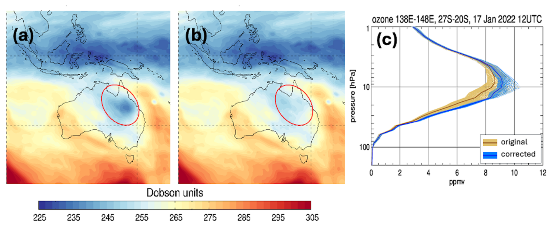
Figure 5 Spatial distribution of Total Ozone Column (TOC) in M2-SCREAM reanalysis data on 17 January 2022 at 06:00 UTC. (a) Assimilation using anomalous OMI V3 TOC retrievals. (b) Assimilation after filtering out the anomalous OMI TOC and re-processing M2-SCREAM. (c) Ozone profiles from the original M2-SCREAM reanalysis data (orange), and from the assimilation that omitted anomalous OMI TOC (blue) on 17 January 2022 at 12:00 UTC.

For BUV aerosol plume retrievals, it is clear from the above discussion that we cannot use aerosol-contaminated BUV ozone data. Instead, for the air density, temperature, and ozone profiles, we have used specially-processed M2-SCREAM reanalysis data. This special processing involves the removal of erroneous OMI-retrieved total ozone columns in the Hunga plume from this reanalysis (both OMI and MLS are on the Aura platform) for the 10 d period of 15–25 January 2022. Figure 5b presents the total ozone map from special reprocessing, which is smoother than the original assimilated ozone columns that show a low anomaly over Northeast Australia (Fig. 5a). Assimilated ozone profiles also show low anomalies in the stratosphere when erroneous OMI TOC values were included (Fig. 5c). Regarding M2-SCREAM temperature profiles, early-January temperatures may be less reliable due to sparsely assimilated H₂O and partial GPS radio-occultation contamination under conditions of extreme moisture (Randel et al., 2023). To assess the reliability of these temperature profiles, we compared the M2-SCREAM temperature profiles using radiosonde data from stations in Australia and New Caledonia (University of Wyoming archive; https://weather.uwyo.edu/upperair/sounding.shtml, last access: 16 October 2025). We selected eight cases in which the relative humidity exceeded 10 % at least once above 15 km, including the 17 January 2022, 00:00 UTC sounding. The M2-SCREAM temperatures agreed with the radiosonde measurements within ∼ 4 K over 15–30 km range, supporting that the reanalyzed M2-SCREAM temperature profiles are sufficiently reliable for interpreting the early Hunga plume conditions.

3 Nadir-BUV aerosol retrieval algorithm

In Sect. 3.1 we introduce BUV measurement and state vectors, focusing on the use of ratioed BUV radiances from adjacent orbits; this section deals with parameterization of the Hunga plume in terms of a pseudo-Gaussian profile shape. We summarize the deployment of the VLIDORT Radiative Transfer (RT) model in the forward model component in Sect. 3.2, with special emphasis on the linearized optical property set-ups required by VLIDORT to generate analytically-derived Jacobians with respect to AOD and peak height. The least-squares inversion model is outlined in Sect. 3.3, and in Sect. 3.4, we discuss the preparation of aerosol optical properties, parameterization of the SO₂ vertical profile, and the use of input ozone profiles from the modified MERRA-2 reanalysis. Section 3.5 is concerned with the algorithm validation using synthetic data.

3.1 State and measurement vectors

Measurement vectors for the retrieval M_meas(λ_i) are ratios of two BUV radiance spectra measured in discrete wavelength channels, $i=\mathrm{1},N_{\mathrm{S}}$ (with associated measurement uncertainties):

$$\begin{array}{}\text{(1)}& M_{\mathrm{meas}}\left({\mathit{\lambda }}_i\right)={\displaystyle \frac{R_{\mathrm{meas}}^{\left(\mathrm{Volc}\right)}\left({\mathit{\lambda }}_i\right)}{R_{\mathrm{meas}}^{\left(\mathrm{Bkgd}\right)}\left({\mathit{\lambda }}_i\right)}}\end{array}$$

In the following, the $R_{\mathrm{meas}}^{\left(\mathrm{Volc}\right)}\left({\mathit{\lambda }}_i\right)$ is a discretized BUV spectrum with a distinct Hunga aerosol signal (e.g., from TROPOMI orbit 22086 or 22087), and $R_{\mathrm{meas}}^{\left(\mathrm{Bkgd}\right)}\left({\mathit{\lambda }}_i\right)$ is a background BUV spectrum (e.g., from TROPOMI orbit 22085) with similar observational angles and wavelength grid. The dimension of the measurement vector, N_S, is variable – this depends on the choice of spectral fitting window and the application of spectral smoothing (if any). For the short spectral fitting window (289–296 nm), there are typically N_S=107 spectral points without smoothing. For measurement random errors we use radiance noise levels from the TROPOMI Level 1B product, assuming that individual spectral measurement errors are uncorrelated. The uncertainty in the radiance ratio is then calculated using error propagation, combining the relative uncertainties of each scene in quadrature and scaling the result by the radiance ratio.

The number of retrieved quantities determines the dimension of the state vector, x. The Hunga aerosol loading profile {E(z)} as a function of altitude z is taken to have a “pseudo-Gaussian” shape (this analytic parameterization is sometimes called a Generalized Distribution Function), characterized by three parameters $\left\{A_{\mathrm{0}},z_{\mathrm{p}},h_{\mathrm{w}}\right\}$. Here, A₀ is the Hunga stratospheric AOD at a fixed reference wavelength λ_ref (taken to be 312 nm), z_p is the plume peak height in [km], and h_w is the half-width-half-maximum of the plume profile (also in [km]). For a 2-parameter retrieval, the state vector is $\mathit{x}=\left\{A_{\mathrm{0}},z_{\mathrm{p}}\right\}$, with h_w treated as a known model parameter (see Sect. 3.4 for more on this quantity). Appendix A contains a description of this pseudo-Gaussian parameterization, including explicit analytic expressions for $E\left(z;A_{\mathrm{0}},z_{\mathrm{p}},h_{\mathrm{w}}\right)$ in terms of the three parameters of interest, and a determination of analytic derivatives $\left\{\frac{\partial E\left(z\right)}{\partial A_{\mathrm{0}}},\frac{\partial E\left(z\right)}{\partial z_{\mathrm{p}}}\right\}$ necessary for deriving analytical layer Jacobian output from the forward model component of the retrieval algorithm.

As noted in Sect. 2.2, ozone, pressure, and temperature profiles are assumed to be accurately known from the re-processed M2-SCREAM reanalysis, independent of Hunga aerosols. We also evaluated the potential impact of air-density variations on Rayleigh scattering (Bodhaine et al., 1999) and ozone absorption (Guo and Lu, 2006), which may not be fully captured by the M2-SCREAM reanalysis during the initial days following the eruption. For a given set of TROPOMI BUV radiances, the following tests were conducted:

• The original atmospheric temperature and pressure profiles were perturbed while maintaining a fixed ozone profile.

• The original atmospheric ozone profile was perturbed while maintaining fixed temperature and pressure profiles.

• All three original profiles were replaced to observe their combined influence.

Representative retrievals were performed for each of these combinations of forward model input parameters to assess the impact of these variations on retrieval results. The replacement of the ozone profile generated the greatest influence; hence, particular attention was given to defining this profile for each TROPOMI scene. However, differences in atmospheric density profiles due to changes in temperature and pressure produced only minor effects on the aerosol retrievals.

3.2 Forward model radiative transfer (RT) and analytic jacobians

Next, we consider the forward-model RT simulation of the ratioed BUV spectra. The retrieval algorithm requires forward-model Jacobians with respect to state vector elements; here, the 2-parameter vector $\mathit{x}=\left\{A_{\mathrm{0}},z_{\mathrm{p}}\right\}$. In general, the forward model will generate simulations M_sim(λ_i) to match the measured vector in Eq. (1). This requires two RT simulations: $R_{\mathrm{sim}}^{\left(\mathrm{Bkgd}\right)}\left({\mathit{\lambda }}_i\right)$ is the RT calculation for a background atmospheric scenario, and $R_{\mathrm{sim}}^{\left(\mathrm{Volc}\right)}\left({\mathit{\lambda }}_i\right)$ is RT simulation with similar geometry, but including volcanic plume. In addition to M_sim(λ_i), the forward model must also generate Jacobians with respect to the aerosol parameters:

$$\begin{array}{}\text{(2)}& \begin{array}{rl}K\left({\mathit{\lambda }}_i\right)& \equiv \left[{\displaystyle \frac{\partial M_{\mathrm{sim}}\left({\mathit{\lambda }}_i\right)}{\partial A_{\mathrm{0}}}},{\displaystyle \frac{\partial M_{\mathrm{sim}}\left({\mathit{\lambda }}_i\right)}{\partial z_{\mathrm{p}}}}\right]\\ & ={\displaystyle \frac{\mathrm{1}}{R_{\mathrm{sim}}^{\left(\mathrm{Bkgd}\right)}\left({\mathit{\lambda }}_i\right)}}\cdot \left[{\displaystyle \frac{\partial R_{\mathrm{sim}}^{\left(\mathrm{Volc}\right)}\left({\mathit{\lambda }}_i\right)}{\partial A_{\mathrm{0}}}},{\displaystyle \frac{\partial R_{\mathrm{sim}}^{\left(\mathrm{Volc}\right)}\left({\mathit{\lambda }}_i\right)}{\partial z_{\mathrm{p}}}}\right].\end{array}\end{array}$$

We use the VLIDORT discrete-ordinate RT model for simulating polarized multiple scattering BUV radiance spectra (Spurr, 2006; Spurr and Christi, 2019) for the two forward-model calculations required. $R_{\mathrm{sim}}^{\left(\mathrm{Bkgd}\right)}\left({\mathit{\lambda }}_i\right)$ is a simulation for a Rayleigh scattering atmosphere with O₃ absorption, and no aerosols or SO₂; the O₃ profile is from re-processed M2-SCREAM reanalysis as described in Sect. 2.2. The major advantage with VLIDORT is its ability to generate not only the radiance fields, but also any set of analytically-derived layer Jacobians (weighting functions) with respect to atmospheric or surface parameters.

Aerosol optical properties are required for the $R_{\mathrm{sim}}^{\left(\mathrm{Volc}\right)}\left({\mathit{\lambda }}_i\right)$ simulation based on a pseudo-Gaussian Hunga aerosol plume loading; for this, we use a linearized Mie scattering model (Spurr et al., 2012) to develop these properties from assumed knowledge of Hunga aerosol microphysical quantities (refractive index, particle size distribution parameters). Details of the aerosol optical property Mie derivations are found in Sect. 3.4, along with a discussion of other atmospheric constituent profiles (in particular, O₃ and SO₂). VLIDORT requires total optical properties (i.e., extinction optical thickness, single scattering albedo, and scattering phase matrix) for each vertical layer and their corresponding linearization to compute the Jacobians (see Appendix B for details).

3.3 Inverse model

The retrieval inverse model is an iterative damped non-linear least-squares minimization using a modified version of the Levenberg-Marquardt (L-M) algorithm (LMA) (Marquardt, 1963) with variable step-size (see e.g., Chong and Zak, 2001). If x_m is the state vector at iteration m, then the estimate for the state vector at the next iteration is given by:

$$\begin{array}{}\text{(3)}& \begin{array}{rl}{\mathit{x}}_{m+\mathrm{1}}& ={\mathit{x}}_m+{\mathit{\alpha }}_m{\left({\mathbf{K}}^{\mathrm{T}}{\mathbf{S}}_{\mathit{ϵ}}^{-\mathrm{1}}\mathbf{K}+{\mathit{\mu }}_m\mathbf{I}\right)}^{-\mathrm{1}}\\ & {\mathbf{K}}^{\mathrm{T}}{\mathbf{S}}_{\mathit{ϵ}}^{-\mathrm{1}}\left({\mathit{y}}_{\mathrm{meas}}-\mathit{F}\left({\mathit{x}}_m\right)\right)\end{array}\end{array}$$

Here, K is the Jacobian matrix which has row vector K(λ_i) for wavelength λ_i in the fitting window as seen in Eq. (2), y_meas is the measurement vector with entries M_meas(λ_i) (Eq. 1), F(x_m) is the forward-model simulated measurement vector with entries M_sim(λ_i) of the same form as that in Eq. (1), S_ϵ is the measurement and forward-model error covariance matrix (here considered diagonal), and I is the identity matrix. The “T” superscript denotes matrix transpose. This inversion scheme is a form of the maximum-likelihood (ML) method (Rodgers, 2000).

The L-M damping parameter μ_m is adjusted as needed at each iteration in order to ensure the approximation to the Hessian matrix $({\mathbf{K}}^{\mathrm{T}}{\mathbf{S}}_{\mathit{ϵ}}^{-\mathrm{1}}\mathbf{K}+{\mathit{\mu }}_m\mathbf{I})$ in Eq. (3) remains positive definite. This ensures that the shape of the cost-function approximation we are seeking to minimize during that iteration is “bowl-shaped”, and that the negative of the gradient ${\mathbf{K}}^{\mathrm{T}}{\mathbf{S}}_{\mathit{ϵ}}^{-\mathrm{1}}({\mathit{y}}_{\mathrm{meas}}-\mathit{F}({\mathit{x}}_m\left)\right)$ in Eq. (3) points in a direction to descend into the bowl.

The step-size α_m is sometimes determined by a line search, in order to guarantee the cost function approximation is minimized at each iterative step; however, this procedure would be too numerically expensive in our retrieval. Instead, in order to ensure that A₀ and z_p remain in physical parameter space at each iteration step, we simply halve the step size repeatedly until this physicality condition is satisfied (starting at α_m=1).

Convergence is reached when relative differences in state-vector elements between adjacent iterations are all below a threshold criterion (10⁻² in our case), and/or when the cost-function itself reaches a clear minimum in fitting space. Spectral points are $\left\{{\mathit{\lambda }}_i\right\},i=\mathrm{1},\mathrm{\dots }{N}_{\mathrm{s}}$, where the number of points N_s depends on the selection of TROPOMI measurements in UV band 1. With two parameters (A₀ and z_p), matrix K in Eq. (3) has dimension N_s×2.

In addition to the above, to obtain better estimates of uncertainties on the retrieved state vector elements A₀ and z_p, a facility was implemented to modify the original standard deviations from the measurement and forward-model error covariance matrix S_ϵ used in retrieval (which is often based initially on measurement characteristics alone such as signal-to-noise ratio (SNR)). This was done as follows. As part of each original retrieval, a chi-square diagnostic ${\mathit{\chi }}^{\mathrm{2}}=[{\mathit{y}}_{\mathrm{meas}}-\mathit{F}(\mathit{x}\left){]}^{\mathrm{T}}{\mathbf{S}}_{\mathit{ϵ}}^{-\mathrm{1}}\right[{\mathit{y}}_{\mathrm{meas}}-\mathit{F}\left(\mathit{x}\right)]$ is produced. If the value of chi-square for the retrieval is too large – indicating that the estimated mismatch in actual measurements y_meas versus forward-model-simulated measurements F(x) is generally too large relative to that assumed using the original standard deviations in S_ϵ – then the expected value of chi-square for the retrieval (i.e., the number of measurements N_s used in the retrieval minus one), along with y_meas, the final values of F(x) from the original retrieval, and the original standard deviations used in S_ϵ, are used to compute an additional contribution to the estimated standard deviation of measurement/forward model error for each measurement. These contributions account for the influence of unknown sources of measurement and/or forward model error. These values are then added to the original measurement standard deviations on the diagonal of S_ϵ and the retrieval is then re-run using the more realistic combined standard deviations of measurement and forward-model error. With this procedure, retrieved values of the state vector elements often do not change significantly, but their estimated uncertainties are often more realistic (i.e., larger), along with improved chi-square diagnostics.

3.4 Forward-model setups

3.4.1 Vertical profiles

As noted in Sect. 2.2, we use specially-processed ozone and temperature assimilated vertical profiles (reprocessed M2-SCREAM) – this data set contains pressure, temperature and ozone volume mixing ratios specified for a 72-layer vertical grid at 1–2 km vertical resolution in the stratosphere. This 72-layer grid forms the basis for the atmospheric stratification. We have imposed a finer vertical resolution for the Hunga aerosol plume (typically 0.25 km is sufficient), in order to properly characterize the pseudo-Gaussian plume shape. Baseline retrievals are done assuming the aerosol peak height z_p to be between 24 and 34 km, in general above the ozone density peak at ∼ 25 km. We performed a sensitivity study allowing the minimum value of z_p to be 20 km; we found that this had a negligible impact on the total aerosol mass retrieval. Figure 6 illustrates the assumed aerosol and ozone profile distributions, along with CALIOP overpasses from 17 January 2022. In particular, the CALIOP daytime overpass at 05:29 UTC shows a narrow plume at 30 km (Fig. 6c, see also the CALIOP nighttime overpass at ∼ 16:20 UTC (Fig. 6d) and ∼ 17:59 UTC (Fig. 6e)); based on this, we estimate a plume half-width of ∼ 0.4 km, and this value was assumed throughout the retrievals discussed in the paper.

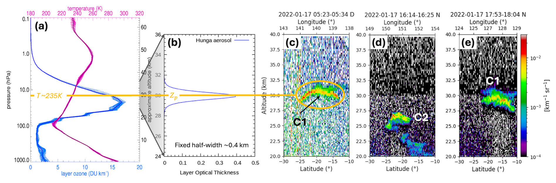
Figure 6 (a) Ozone and temperature profiles from the reprocessed M2-SCREAM reanalysis data on 17 January 2022, at 12:00 UTC. (b) Example of a modelled aerosol profile assuming a Gaussian-like shape with fixed half-width ∼ 0.41 km (see Appendix A). (c) Total attenuated backscatter at 532 nm measured by CALIOP during daytime (∼ 05:29 UTC) on 17 January 2022. Same as Fig. 6c but for nighttime measurements at (d) ∼ 16:20 UTC and (e) ∼ 17:59 UTC.

3.4.2 Optical properties

The Mie code is an integral part of the forward model; we use the code to generate aerosol optical properties in the UV range, based on microphysical inputs typical for stratospheric sulfuric acid solution spherical droplets (Palmer and Williams, 1975; Beyer et al., 1996). These inputs include laboratory measurements of complex index of refraction at a reference wavelength of 312 nm, for a binary sulfuric acid ${\mathrm{H}}_{\mathrm{2}}{\mathrm{SO}}_{\mathrm{4}}/{\mathrm{H}}_{\mathrm{2}}\mathrm{O}$ solution. We have chosen two values for the real part of the refractive index (n_r=1.39 and n_r=1.47), which represent the lower and upper limits of the laboratory measurements (Beyer et al., 1996) corresponding to low (w=0.291) and high (w=0.765) acid mass fractions of the binary water-sulfuric acid solutions (Myhre et al., 1998). This wide range for the real part of the refractive index reflects the plume composition simulated by NASA Goddard Earth Observing System (GEOS) Earth system model (see Appendix F), i.e., H₂SO₄ wt % spanning roughly 40 %–70 % (core values ∼ 40 %) and thus reasonably bracketing the ∼ 30 %–80 % range. We assumed n_r values to be spectrally constant in the UV spectral fitting window. The imaginary part of the refractive index can be neglected in the UV, visible and near infrared wavelengths (Beyer et al., 1996); this was set to a value of 10⁻⁴ throughout.

Besides complex refractive index values {n_r,n_i} = {1.39–1.47, 10⁻⁴}, two parameters – the fine mode radius (r_g∼0.14 µm) and the standard deviation (S_g=1.545) – were chosen to characterize the unimodal lognormal particle number size distribution of the Hunga aerosol; these parameters were derived from the Lucinda AERONET level 1.5 (Holben et al., 1998) sun-sky radiance inversions (Dubovik and King, 2000) during Hunga cloud overpass (Boichu et al., 2023). An initial call to the Mie program is required to generate the extinction coefficient Q_ext(λ₀) at reference wavelength λ₀=312 nm, and this is followed by more calls to the Mie code at every wavelength λ_i, i=1, N_S to generate the full set of aerosol optical properties (spectral extinction, single scattering albedo, elements of the scattering matrix) required as input to the VLIDORT optical setup. The deployment of these Mie properties in the VLIDORT setup is discussed in Appendix B.

Ozone cross-sections and temperature dependence are taken from laboratory measurements (Brion et al., 1993). The original high-spectral resolution data are pre-convolved with pixel-specific spectral response functions and then spline-interpolated to TROPOMI wavelengths, λ_i, i=1, N_S. SO₂ cross-sections are taken from Bogumil et al. (2003) and are also pre-convolved and interpolated. Both cross-section data sets exhibit temperature dependencies parameterized by quadratic functions, utilizing re-processed M2-SCREAM assimilated temperature profiles (Fig. 6a). Rayleigh scattering cross-sections and depolarization ratios are taken from a standard source (Bodhaine et al., 1999).

3.4.3 Radiative transfer aspects

In the UV spectral region below 300 nm, single scattering (SS) dominates the radiative transfer (RT) for an aerosol-free stratosphere, with light penetration depths related to the wavelength-dependent ozone and SO₂ absorption peaks. With mid-stratospheric Hunga aerosols present, multiple scattering (MS) becomes more important, and it is necessary to run VLIDORT in full scattering mode (SS + MS). The number of discrete ordinates is set at 8 in the polar angle half space; we have found that this is sufficient for treating the Hunga aerosol scattering accurately, provided the delta-M scaling approximation is in force. VLIDORT is run in linear polarization mode (Stokes-vector components I, Q, U); circular polarization is neglected.

3.5 Validation with synthetic data

We calculated Hunga BUV synthetic radiances using the NASA OMI spectral simulator software, based on geophysical conditions for 17 January 2022. Simulations were performed with and without aerosols to develop synthetic radiance ratios, which were then used as input to the Hunga inversion tool, the purpose being to evaluate the impact of changing the ozone profile and the Hunga aerosol layer height and AOD. These tests helped to develop confidence in the forward and inverse models used in the real Hunga retrievals.

In addition, a number of tests were carried out to obtain a sense of the retrieval's sensitivity to (1) the half width at half maximum (HWHM) of the ascribed aerosol plume profile, (2) profiles of atmospheric density and ozone, (3) parameters governing the aerosol particle size distribution [e.g. mode fraction (assuming a bimodal particle size distribution), mode radius, refractive index (real & imaginary parts)], (4) the spectral window chosen for retrieval, and (5) the influence of the initial state vector guess on retrieval convergence. These tests were used as a guide to aspects of the retrieval which demanded further attention during the process of refining the retrieval algorithm.

To further verify the fidelity of the retrieval algorithm itself, we performed a set of closed-loop validation tests using synthetic radiance spectra generated by the forward model. Each test used a pre-defined state vector ${\mathit{x}}_{\mathrm{true}}=\mathit{\{}\text{AOD},z_{\mathrm{p}}\mathit{\}}$ to represent typical Hunga plume conditions. Two cases were examined: (1) a retrieval based on noise-free synthetic spectra to ensure that the algorithm could reproduce the known state (x_ret≈x_true), and (2) a retrieval using spectra with added random noise levels representative of TROPOMI UV band 1 measurements to assess retrieval robustness under realistic conditions. In both cases, the retrieved parameters converged closely to the true inputs, demonstrating that the Hunga retrieval framework is stable and internally consistent. The noise-added tests also showed slightly larger retrieval uncertainties, as expected, but without systematic bias in AOD or z_p. Overall, the results increased confidence in the forward and inverse model configurations used in the actual Hunga plume retrievals.

4 Hunga aerosol retrieval results

To facilitate Hunga sulfate aerosol mass estimation, we have selected TROPOMI measurements from 17 January 2022, taken at ∼ 01:30 pm local time (03:30 UTC), because by that time (∼ 47 h after the eruption) the SO₂ and sulfate aerosol clouds have completely separated from the ash and ice clouds (see Fig. 1c from Sellitto et al., 2022), but the volcanic clouds were still above the ozone density peak at ∼ 25 km. The absence of UV-absorbing ash is confirmed by low values of the TROPOMI-derived UV absorbing aerosol index. As noted in Sect. 2.1, Hunga plume pixels have been discriminated using a cloud screening index (CSI) value greater than > 1.1, where CSI is the BUV radiance ratio with the background orbit (22085) at 296 nm (see Appendix C).

4.1 Aerosol peak height retrievals

Hunga aerosol peak heights z_p were retrieved using both lower (n_r=1.39) and upper (n_r=1.47) bounds of the real part of the refractive index; these values provide an uncertainty range for Hunga z_p retrievals. Figure 7a shows z_p retrieved using the upper-bound index (n_r=1.47). The highest values of z_p > 30 km were retrieved in the western part of the plume from orbit 22087. The lower z_p values (∼ 25 km) were retrieved in the eastern part from orbit 22086. This west–east contrast is consistent with previous studies distinguishing the western aerosol- and water-rich cloud (C1) and the eastern SO₂-rich cloud (C2) (Carn et al., 2022; Legras et al., 2022). The C1 cloud likely experienced faster SO₂-to-sulfate conversion and stronger water-driven radiative cooling, which contributed to its more rapid descent compared to that for C2, as noted in previous analyses (Legras et al., 2022; Sellitto et al., 2022). This difference is largely explained by the strong stratospheric easterly wind gradient in the 20–40 km altitude range. This interpretation is supported by the trajectory analysis presented in Appendix D, which uses assimilated wind data from the MERRA-2 reanalysis. The higher the altitude, the stronger the easterly winds, so those parts of the C1 cloud at z_p $\sim \mathrm{30}\pm \mathrm{1}$ km were advected westward more quickly than the lower parts (Sadeghi et al., 2025). By contrast, the C2 cloud, centered near $z_{\mathrm{p}}\sim \mathrm{25}\pm \mathrm{1}$ km in the eastern sector, showed slower westward advection consistent with a weaker easterly wind field at these lower stratospheric levels.

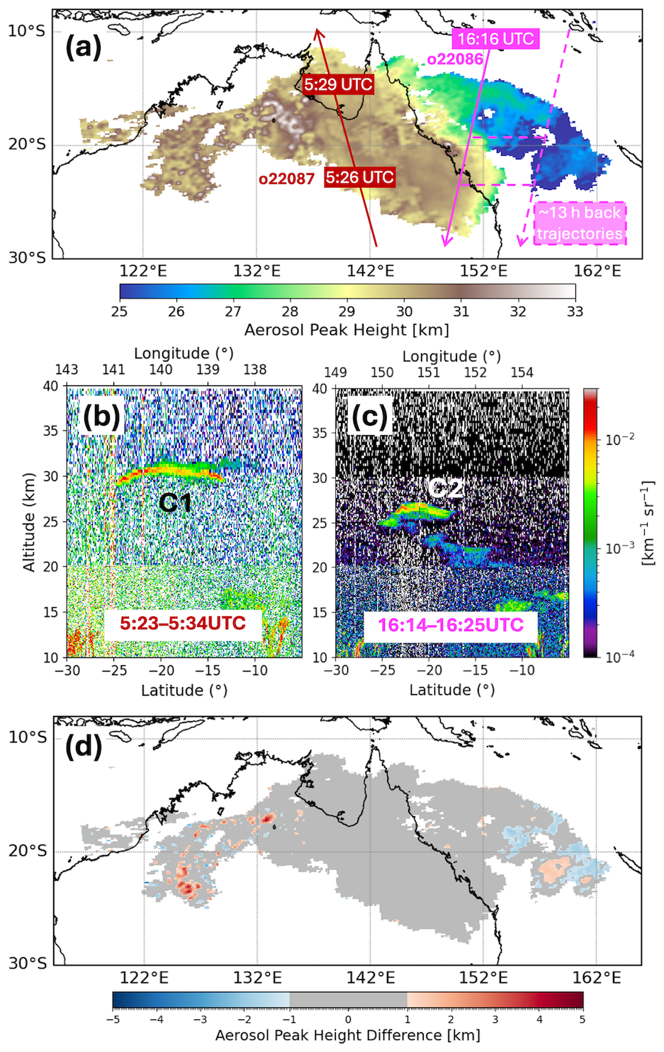
Figure 7 (a) Retrieved aerosol plume peak height z_p [km] assuming upper limit sulfate solution concentration 76.5 wt % (n_r=1.47), from TROPOMI orbits 22086 (∼ 03:20 UTC) and 22087 (∼ 05:00 UTC) on 17 January 2022. (b) The CALIOP attenuated backscatter during daytime (∼ 05:23–05:34 UTC) with the ground track shown in panel (a) with the solid red line. (c) Same as (b) but for a nighttime track (∼ 16:14–16:25 UTC), which is shown with the solid magenta line in panel (a). The dashed magenta line shows a back-trajectory matchup between nighttime CALIOP measurements and daytime TROPOMI Hunga aerosol retrievals. (d) Difference in retrieved z_p assuming low solution concentration ∼ 30 wt % (n_r=1.39) compared to high n_r=1.47 retrieval (a).

We compared the TROPOMI aerosol peak heights z_p retrieved from orbit 22086 at ∼ 03:30 UTC and orbit 22087 at ∼ 05:00 UTC with the CALIOP daytime overpass at 05:27–05:29 UTC (Fig. 7b) and later nighttime overpass at ∼ 16:16 UTC (Fig. 7c). Examining the daytime CALIOP data, we see that the average height of the C1 cloud is close to 30 km. The z_p heights retrieved from TROPOMI orbit 22087, ∼ 30 min prior to the CALIOP observations, match within ∼ 1 km. A second validation was obtained with the CALIOP nighttime overpass at 16:16 UTC (solid magenta line), where matchup between CALIOP and TROPOMI pixels within the C2 part of the Hunga plume (shown with the dashed magenta line) can be achieved with 13-h back trajectories (Appendix D).

TROPOMI z_p ∼ 30 km over the Northeastern part of Australia also agrees with the geometric top height retrievals from the Multi-angle Imaging Spectro-Radiometer (MISR) aboard NASA's Terra satellite. On 17 January 2022, MISR observed the Hunga aerosol plume off the Northeast coast of Australia at ∼00:25 UTC, with retrieved height of 27–30+ km a.s.l. (30 km is the maximum allowed retrieval height in the MINX (MISR INteractive EXplorer) stereo-height retrieval (Kahn et al., 2024)).

Figure 7d shows the absolute difference in z_p retrieved using the lower-bound refractive index (n_r=1.39) relative to n_r=1.47 scenario. The average difference is 0.03 ± 0.8 km, indicating generally low sensitivity to the refractive index assumptions. Notably, in the central dense part of the plume, most areas fall within a ± 1 km difference range (shaded in gray). However, larger localized differences of up to ± 2 km were observed in the eastern part of the plume above the Coral Sea. These discrepancies may be due to the low altitude of the Eastern part of the plume, close to the assumed plume boundary (24 km). The differences in z_p up to ∼ 4 km were found in areas with thin aerosol layers, likely due to reduced sensitivity in such cases. Overall, differences in z_p values retrieved using extreme refractive index assumptions fall within the expected range.

4.2 Aerosol optical depth (AOD) retrievals

Without prior information about Hunga aerosol sulfuric acid (${\mathrm{H}}_{\mathrm{2}}{\mathrm{SO}}_{\mathrm{4}}/{\mathrm{H}}_{\mathrm{2}}\mathrm{O}$) aqueous solution concentration we repeated AOD retrievals using low (n_r=1.39) and high (n_r=1.47) values of the real part of the refractive index, n_r, which correspond to a plausible range for sulfuric acid concentrations (∼ 26 wt % to ∼ 79 wt %) (Beyer et al., 1996; Toon and Pollack, 1973). Figure 8 shows TROPOMI-retrieved AOD at reference wavelength λ₀=312 nm for the upper limit of the refractive index (n_r=1.47) and the percentage difference in results between the two n_r scenarios. The highest AOD values (up to ∼ 5.0) were retrieved over the Coral Sea (C2 cloud), where the densest portion of the volcanic plume was concentrated at lower plume altitudes around 25 km (see Fig. 8a). As the plume was transported westward across northern Australia, a secondary maximum in aerosol density was located over Western Queensland (C1 cloud), with AOD values as high as 3. Further westward, AOD values gradually decreased over Northeast Australia coinciding with a higher z_p values (>30 km).

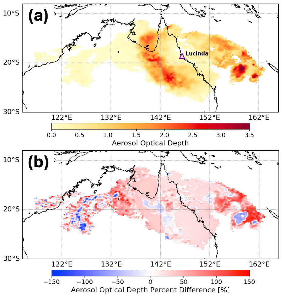
Figure 8 (a) Retrieved TROPOMI Aerosol Optical Depth (AOD) at 312 nm assuming n_r=1.47 at 312 nm for orbits 22086 and 22087. The location of the Lucinda AERONET site is marked with a triangle. (b) Percentage difference in AOD retrievals using low sulfate solution concentration (refractive index n_r=1.39) relative to the AOD retrieval using high solution concentration (n_r=1.47).

The comparison (Fig. 8b) shows that retrieved AODs for low aqueous sulfuric acid solution concentration (n_r=1.39) are generally higher than those AODs for high solution concentration (n_r=1.47), with a mean percent difference of ∼ 30 %; this provides an estimate of the AOD systematic retrieval error associated with uncertainties in the refractive index assumptions. The largest differences were found in regions with optically thick plumes, particularly over the Coral Sea, where the aerosol peak height was close to the assumed low limit of $min\left(z_{\mathrm{p}}\right)\sim$ 24 km – that is, close to the ozone density peak.

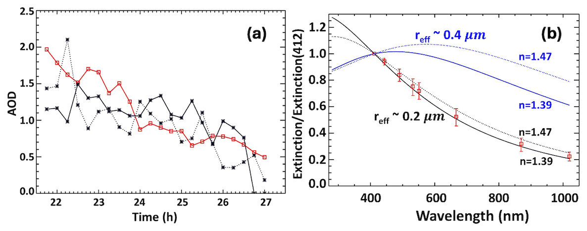
Figure 9 Panel (a) red line shows 15-minute averages of the AERONET AOD₄₁₂ measurements at 412 nm at Lucinda site started at 21:45 UTC on 16 January 2022 (local morning time) and continued until ∼ 03:00 UTC on 17 January 2022. The horizontal scale is given in hours elapsed from 00:00 UTC on 16 January. We subtracted a background tropospheric AOD₄₁₂ of 0.1 measured on the previous days. The black dotted (solid) line represents the average of TROPOMI AOD₄₁₂ retrievals assuming n_r=1.47 (n_r=1.39) for pixels affected by Hunga aerosols that pass within 10 km of the Lucinda site. We adjusted TROPOMI retrieved AODs at 312 nm to the AERONET measured AOD₄₁₂ using theoretical Hunga aerosol extinction spectral dependence shown in panel (b) for effective radius r_eff∼0.2 µm (black curves). Panel (b) The red squares show the average spectral dependence of the AERONET AOD measurements during Hunga plume overpass shown in panel (a) and normalized to AOD₄₁₂ at 412 nm. The 3× standard deviation of the ratios $\mathrm{AOD}/\mathrm{AOD}$₄₁₂ is shown as a vertical bar (±3σ). The black solid (dotted) curve shows the theoretical extinction ratio from Mie calculations assuming n_r=1.39 (n_r=1.47) and effective radius r_eff∼0.2 µm. The blue curves show similar extinction ratios using a larger r_eff∼0.4 µm retrieved in March 2022 by the solar occultation SAGE-III instrument aboard the International Space Station (Duchamp et al., 2023). It is clear that TROPOMI retrieval assumption of r_eff∼ 0.2 µm is consistent with the AERONET spectral AOD measurements during Hunga plume overpass on 17 January 2022.

To validate our TROPOMI AOD retrievals, we compared them with AERONET direct-sun AOD measurements (Holben et al., 1998) from the Lucinda coastal site (18.5198° S; 146.3861° E; elevation: 8.0 m) during the Hunga plume overpass from ∼ 21:00 UTC on 16 January to ∼ 03:00 UTC on 17 January (Fig. 9). The Lucinda site is located ∼ 6 km offshore in the tropical coastal waters of the Great Barrier Reef, and background AOD at this site is typically very small. Based on AERONET values of aerosol microphysical parameters and assumed values of refractive index, we used the Mie code to convert our retrieved TROPOMI AOD at 312 nm to corresponding quantities at 412 nm; this is the shortest AOD wavelength for AERONET measurements at Lucinda (Fig. 9b). We also subtracted tropospheric AOD contributions of 0.1, as measured by AERONET on previous days to the Hunga plume overpass.

Using the NASA Goddard trajectory model (see Appendix D), we calculated the backward movement of air parcels starting from TROPOMI AOD retrievals from orbit 22087 (overpass at 05:00 UTC) and from 22086 (overpass at 03:15 UTC). We averaged all TROPOMI AOD retrievals from those parcels that pass within 10 km of the Lucinda site and compared them with the AERONET AOD measurements averaged over a 15-minute interval (Fig. 9a). We see that average retrieved AOD values show good qualitative agreement with the AERONET AOD measurements. Quantitatively, the retrievals assuming n_r=1.47 (black dotted curve) showed a median difference of 0.25 (mean: 0.3) relative to AERONET. For the n_r=1.39 (black solid curve) case, the median difference is similar 0.3 (mean: 0.3). Both TROPOMI and AERONET AODs reached a maximum (over 2) during the local-time morning hours (21:45–23:00 UTC on 16 January) and dropped to ∼ 0.5 after the main part of the Hunga aerosol cloud passed over the station.

TROPOMI AOD retrievals also agree qualitatively with MISR-retrieved AOD${}_{\mathrm{558}}\sim \mathrm{0.7}\pm \mathrm{0.2}$ (1σ) (Kahn et al., 2024), accounting for spectral differences in the aerosol extinction between short UV and mid-visible wavelengths (Fig. 9b). Recent AOD₅₃₂ retrievals from CALIOP nighttime Hunga overpasses estimate somewhat larger AOD₅₃₂ values of $\sim \mathrm{1.24}\pm \mathrm{0.13}$ (1σ) for C1 and $\sim \mathrm{1.01}\pm \mathrm{0.12}$ (1σ) for C2 on 17 January (Duchamp et al., 2025). These CALIOP-derived AOD₅₃₂ values are also consistent with TROPOMI AOD results, considering the spatial heterogeneity of the Hunga plume, the temporal differences between the satellite overpasses, and the spectral differences between the retrievals. A more comprehensive comparison with CALIOP will be conducted in a follow-up study.

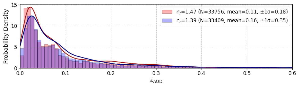
Figure 10 Normalized probability density function of retrieved AOD uncertainties ε_AOD for the Hunga Plume on 17 January 2022. Results are shown for two limiting refractive index values: n_r=1.47 (red) and n_r=1.39 (blue). The number of valid retrievals with AOD > 0.2 (N) and corresponding median and interquartile range (IQR; 25th–75th percentile) are indicated in the legend.

We estimated AOD retrieval uncertainties ε_AOD theoretically using different approaches: (1) taking error estimation from the Hunga retrieval algorithm diagnostic and comparing retrievals using low and high limits of n_r=1.39 and 1.47 as shown in Fig. 10, and (2) comparing AOD retrievals for each Hunga pixel using short (289–296 nm) and extended (289–310 nm) spectral fitting windows (see Fig. 3). We note the following:

Retrieval ε_AOD uncertainties were initially based on TROPOMI radiance measurement noise (SNR) but were later refined incorporating additional contributions derived from chi-square diagnostics accounting for discrepancies between measured and simulated radiance ratios (see Sect. 3.3). Figure 10 shows the normalized probability density distribution of the updated ε_AOD for all pixel retrievals in Hunga plume; this distribution has a long non-Gaussian tail; therefore, we use the median and the interquartile range (IQR; 25th–75th percentile) statistics rather than the mean and the standard deviation to describe an overall AOD uncertainty. The relative ε_AOD greatly increases for small AODs. When restricted to cases with AOD > 0.2, the median ε_AOD∼0.06 and the corresponding IQRs are 0.02(0.03)–0.13 for both n_r cases (Fig. 10). Then normalizing to the retrieved AOD, this median absolute error corresponds to a median percentage error of ∼ 15 %.

To estimate the upper limit of the ε_AOD, we repeated TROPOMI Hunga retrievals using the extended spectral fitting window (289–310 nm) (see Fig. 3) and assuming upper limit of n_r=1.47. With this long fitting window, we obtained AOD values ∼ 16 % lower than those obtained with the “short” window. This reduction is possibly due to increased sensitivity to tropospheric clouds and uncertainties in assumed gas-phase absorbers such as O₃ and SO₂. These comparisons indicate the importance of varying the spectral fitting window to estimate the upper limit of uncertainty of our Hunga aerosol retrievals. On the other hand, using an extended spectral fitting window would permit retrieval of additional aerosol parameters (e.g., effective radius) or gases (e.g., O₃, SO₂), but would require a more complex forward RT model (e.g., including tropospheric cloud correction).

Furthermore, to estimate potential instrument-specific biases we carried out an inter-sensor comparison against the NOAA-20 OMPS Nadir Profiler (NP) based Hunga retrieval; this was conducted using the same short spectral fitting window (289–296 nm) and specially assimilated O₃ profiles (see Appendix E). The retrieved NOAA-20 OMPS-NP AOD values were approximately ∼ 20 % higher than those from our TROPOMI retrievals collocated within six OMPS-NP pixels over Northeast Australia. Based on these estimates, we adopt ε_AOD±20 % as the total percent uncertainty, considering both retrieval and instrument specific errors.

4.3 Aerosol mass retrievals

To convert the retrieved AOD to aerosol column mass m_aer (g m⁻²) we need to know particle mass density, ρ (g cm⁻³), effective radius r_eff (µm), and extinction efficiency $Q_{\mathrm{ext}}=\frac{<\mathrm{Ext}>}{<G>}$, where $<\mathrm{Ext}>$ and $<G>$ are particle size distribution weighted average extinction and geometric cross-sections (Krotkov et al., 1999a, b; Duchamp et al., 2023; Sellitto et al., 2024):

$$\begin{array}{}\text{(4)}& m_{\mathrm{aer}}={\displaystyle \frac{\mathrm{4}}{\mathrm{3}}}{\displaystyle \frac{\mathit{\rho }{r}_{\mathrm{eff}}}{Q_{\mathrm{ext}}}}\mathrm{AOD}\end{array}$$

We assume that the AERONET-retrieved fine-mode effective radius r_eff∼0.22 µm at Lucinda (Fig. 9b) is representative of the whole Hunga plume. To compare with the satellite infrared IASI retrievals, we first assume the same mass density ρ=1.75 g cm⁻³ (Sellitto et al., 2024). This density corresponds to a high sulfuric acid mass fraction w=0.765 at temperature T=233 K (Myhre et al., 1998) and a high value of n_r=1.47 at ∼ 300 nm (Beyer et al., 1996). These values are used in Eq. (3) to produce the spatial distribution of Hunga column aerosol mass m_aer shown in Fig. 11. The column mass spatial distribution has similar features to those in the AOD map (Fig. 8a). Using a BUV radiance ratio filter at 296 nm (CSI > 1.1) to define the plume, we estimate a total plume area $A_{\mathrm{total}}\sim \mathrm{4}\times {\mathrm{10}}^{\mathrm{6}}$ km², and a corresponding total wet aerosol mass M_aer=0.47 Tg, where “wet” denotes aqueous sulfuric acid solution droplets including water uptake at temperature T∼233 K. The maximal m_aer∼0.8 g m⁻² was found over the densest part of the plume over the Coral Sea, as discussed in Sect. 4.2, given that the aerosol column mass values are proportional to the AOD. In the aerosol-rich (C1) part of the plume over Northeast Australia, m_aer increased in value to ∼ 0.5 g m⁻², then decreased to m_aer ∼ 0.05 g m⁻² over the Northwestern part of Australia.

Figure 11 Hunga aerosol column mass, m_aer, on 17 January 2022, assuming aqueous acid solution mass fraction w=0.765, corresponding density ρ∼1.75 g cm⁻³ at T=233 K (Myhre et al., 1998), refractive index, n_r=1.47 (Beyer et al., 1996), and an AERONET retrieved fine-mode effective radius r_eff∼0.22 µm.

Both droplet mass density, ρ, and the refractive index n_r are linked to the assumed sulfuric acid (H₂SO₄) mass fraction (w) in the aerosol solution droplets. Higher sulfuric acid content results in both higher n_r and ρ, and vice versa. To quantify the range of the total wet aerosol mass M_aer, we compared the retrieved m_aer using two limiting (n_r, ρ) pairs:

• for n_r=1.47 and ρ=1.75 g cm⁻³ (w_max=0.765), the integrated total wet aerosol mass M_aer is ∼ 0.47 Tg.

• for n_r=1.39 and ρ=1.25 g cm⁻³ (w_min=0.291), the integrated total wet aerosol mass M_aer is ∼ 0.50 Tg.

These results for M_aer are close; the increase in AOD and opposite decrease Q_ext values are responsible when going from high n_r=1.47 to low n_r=1.39 in Eq. (3). They represent the lower and upper bounds of the retrieved wet aerosol mass, reflecting the impact of microphysical assumptions on the retrieval. We provide a representative estimate of the total wet aerosol mass ∼ 0.5 ± 0.05 Tg; this ∼ 10 % uncertainty includes the AOD retrieval uncertainties discussed in Sect. 4.2.

4.4 Estimate of Hunga sulfate (H₂SO₄) mass fraction and ${\mathrm{H}}_{\mathrm{2}}{\mathrm{SO}}_{\mathrm{4}}/{\mathrm{H}}_{\mathrm{2}}\mathrm{O}$ solution density

The wet aerosol mass M_aer retrieved in our study remains nearly constant: M_aer∼0.5 ± 0.05 Tg for a broad range of assumed sulfuric acid (${\mathrm{H}}_{\mathrm{2}}{\mathrm{SO}}_{\mathrm{4}}/{\mathrm{H}}_{\mathrm{2}}\mathrm{O}$) solution concentrations in Hunga aerosol droplets. Therefore, it is interesting to independently estimate the spatially-averaged sulfuric acid (H₂SO₄) mass fraction w and ${\mathrm{H}}_{\mathrm{2}}{\mathrm{SO}}_{\mathrm{4}}/{\mathrm{H}}_{\mathrm{2}}\mathrm{O}$ solution density ρ. For this, we assume conservation of the total Hunga stratospheric sulfur (S) mass $M_{S_{\mathrm{0}}}$ initially emitted in the gas phase as SO₂, and an exponential SO₂-to-sulfate conversion rate with an e-folding time of τ, to estimate the expected S mass in the aerosol phase M_S,aer at time t (∼ 2 d) after the main eruption on 15 January:

$$\begin{array}{}\text{(5)}& M_{S,\mathrm{aer}}=M_{S_{\mathrm{0}}}\left[\mathrm{1}-e^{(-t/\mathit{\tau })}\right]\end{array}$$

We use reported Hunga gaseous sulfur (S) emissions on 15 January: $M_{S_{\mathrm{0}}}\sim \mathrm{0.21}$–0.24 Tg S (i.e., half the SO₂ mass produced by 15 January eruption) and an e-folding time of τ∼6 d as reported in Carn et al. (2022) to calculate the expected S mass converted to aerosols after ∼ 47 h of transport to be $M_{S,\mathrm{aer}}\sim \mathrm{0.061}$–0.068 Tg S and a gaseous S mass (in SO₂) to be $M_{S,\mathrm{gas}}\sim \mathrm{0.15}$–0.17 Tg S. Within uncertainties, the latter estimate agrees with independent operational TROPOMI stratospheric SO₂ retrievals (Theys et al., 2017) integrated within the Hunga aerosol plume on 17 January (∼ 0.14 Tg S; CSI > 1.1). The average sulfuric acid (H₂SO₄) mass fraction w can be estimated from the ratio of the M_S,aer to the retrieved total wet aerosol mass M_aer∼0.5 Tg, by accounting for their molar weight ratio: (MW_S∼ 32 g mol⁻¹) and H₂SO₄ $({\mathrm{MW}}_{{\mathrm{H}}_{\mathrm{2}}{\mathrm{SO}}_{\mathrm{4}}}\sim \mathrm{98}$ g mol⁻¹):

$$\begin{array}{}\text{(6)}& w={\displaystyle \frac{M_{S,\mathrm{aer}}}{M_{\mathrm{aer}}}}{\displaystyle \frac{{\mathrm{MW}}_{{\mathrm{H}}_{\mathrm{2}}{\mathrm{SO}}_{\mathrm{4}}}}{{\mathrm{MW}}_S}}\end{array}$$

Applying this approach, we estimate the Hunga sulfuric acid mass fraction to be w∼0.37–0.42 with an average value of w∼0.4 and corresponding ${\mathrm{H}}_{\mathrm{2}}{\mathrm{SO}}_{\mathrm{4}}/{\mathrm{H}}_{\mathrm{2}}\mathrm{O}$ solution density: ρ∼1.34 g cm⁻³ at Hunga temperature T∼233 K based on laboratory measurements of Myhre et al. (1998). These new estimates based on Hunga stratospheric S mass balance are consistent with the physics-based sulfate (H₂SO₄) weight percent (wt %) simulation of Hunga aerosols using the NASA Goddard Earth Observing System Chemistry Climate Model (GEOS CCM) with the Community Aerosol and Radiation Model for Atmospheres (CARMA) similar to Case et al. (2023): H₂SO₄∼40 wt %–60 wt % (i.e., w∼0.4–0.6) and ρ∼1.3–1.4 g cm⁻³ (see details in Appendix F).

4.5 Comparison with Infrared SO₂ measurements

Sellitto et al. (2024) reported retrievals of SO₂ and sulfate aerosol mass in the Hunga plume based on mid-IR IASI measurements. Their study noted that SO₂ and sulfate aerosol have overlapping spectral signatures in the IR, which can lead to large uncertainties in the co-retrieval of these species in volcanic plumes; however, the potential impact of collocated water vapor on the IR retrievals was not addressed. In their paper, the equation used to derive sulfate mass from IASI measurements of mid-IR AOD is identical to that used here (Eq. 4) but is based on the measured mid-IR AOD and average extinction efficiency (Q_ext) calculated at mid-IR wavelengths (∼8.5 µm). Sellitto et al. (2024) also assumed a sulfate aerosol mass density of ρ=1.75 g cm⁻³ which corresponds to the upper limit of the sulfuric acid solution concentration w=0.765 at temperature T=233 K (Myhre et al., 1998). Additional uncertainties arise from the range of possible particle size distributions (r_eff∼0.25–0.45 µm) in the Hunga aerosol plume (Boichu et al., 2023; Duchamp et al., 2023).

These authors report a maximum Hunga sulfate aerosol mass loading of 1.6±0.5 Tg, but the peak loading was measured later in the year (August-September 2022). On 17 January 2022, the IASI-derived sulfate aerosol mass reported in Sellitto et al. (2024) is ∼ 0.2 Tg, with a large uncertainty (estimates range up to ∼ 0.8 Tg). Our BUV-based wet aerosol mass of M_aer∼0.5 Tg is thus broadly consistent with these IR retrievals, given the uncertainties on the assumed particle size distribution. In contrast, a larger discrepancy is apparent in the SO₂ retrievals: on 17 January, the IASI-based SO₂ mass is ∼ 0.75 Tg (range: ∼ 0.4–1.1 Tg), compared to a total BUV SO₂ mass of ∼ 0.4 Tg (note that this is the total retrieved SO₂ mass on 17 January, not the SO₂ collocated with the Hunga aerosol plume discussed in Sect. 4.4). Furthermore, the IASI-based SO₂ mass reached a maximum of ∼ 1 Tg (range: ∼ 0.7–1.2 Tg) on 19 January 2022 (Sellitto et al., 2024), whereas the BUV SO₂ mass was observed to decrease after 17 January (e.g., Carn et al., 2022).

Sadeghi et al. (2025) also retrieved Hunga SO₂ mass using CrIS IR measurements in combination with the VOLCAT (VOLcanic Cloud Analysis Toolkit) framework and HYSPLIT-based trajectory analysis to assess SO₂ transport and decay patterns. On 16 January 2022, Sadeghi et al. (2025) reported a CrIS-derived SO₂ mass of ∼ 0.4 Tg, which is consistent with the BUV SO₂ mass reported in Carn et al. (2022).

The reasons for these discrepancies remain unclear. It is possible that the BUV operational SO₂ measurements were more strongly impacted by the presence of optically thick aerosol; we also propose that the impact of Hunga water vapor on the IR SO₂ and sulfate mass retrievals merits further consideration.

5 Summary and conclusions

The 15 January 2022 eruption of the submarine Hunga volcano was a unique volcanic event in the ∼ 50 years since the beginning of the satellite remote sensing era. This powerful eruption was the largest since Pinatubo in 1991, but unlike the SO₂-rich Pinatubo emissions, Hunga injected a volcanic plume dominated by water vapor, with relatively low SO₂ content, to altitudes as high as the lower mesosphere. Although the Hunga eruption has been studied intensively from a number of remote sensing perspectives, in this work we present a novel retrieval of Hunga aerosol optical depth (AOD) and layer peak height (z_p) using short ultraviolet (λ<300 nm) solar backscatter (BUV) band 1 radiance measurements from the TROPOspheric Monitoring Instrument (TROPOMI) on board ESA/Copernicus Sentinel 5 precursor (S5P) satellite and the Ozone Mapping and Profiling Suite- Nadir Profiler (OMPS-NP) on board the National Oceanic and Atmospheric Administration (NOAA-20) satellite. These unique BUV retrievals allow us to detect and characterize total mass and sulfuric acid concentration of Hunga sulfate aerosols that moved across the Southwest Pacific and Australia on 17 January 2022, about 47 h after the 15 January eruption.

We retrieve AOD and z_p by fitting hyperspectral BUV radiance ratios in a narrow spectral window restricted to 289–296 nm, chosen in order to reduce interference from tropospheric clouds while highly sensitive to stratospheric aerosols located above ozone peak altitude. The retrieval employs radiative transfer calculations from the Vector Linearized Discrete Ordinate Radiative Transfer (VLIDORT) forward model. We assume a single Hunga aerosol layer composed of polydisperse sulfuric acid spherical particles embedded in a Rayleigh atmosphere with a known ozone profile. The ozone profile is supplied from a version of the Modern-Era Retrospective analysis for Research and Applications, version 2 (MERRA-2) Stratospheric Composition Reanalysis of the Microwave Limb Sounder (MLS) on board NASA Earth Observing System-chemistry (EOS Aura) satellite – produced by NASA's Global Modeling and Assimilation Office using a stratospheric chemistry model and MERRA-2 meteorology. We also include SO₂ layer, which coincides spatially with the retrieved aerosol vertical profile, and with the total loading normalized to the stratospheric SO₂ vertical column density from the operational TROPOMI SO₂ product. We validate our AOD retrievals against ground-based AERONET direct-sun AOD measurements, and z_p retrievals against Cloud-Aerosol Lidar with Orthogonal Polarization (CALIOP) overpasses using Lagrangian trajectory modeling.

We use TROPOMI-retrieved AOD to estimate a Hunga sulfate wet aerosol mass (i.e., sulfuric acid (H₂SO₄) solution droplets, including water uptake) to be ∼ 0.5 ± 0.05 Tg on 17 January, just two days after the main eruption. This mass estimate is consistent with our previous BUV retrievals of Hunga sulfur dioxide (SO₂) emissions (∼ 0.4–0.5 Tg SO₂ from 15 January eruption) and rapid conversion of SO₂ to sulfate aerosol (e-folding time ∼ 6 d).

Based on these BUV aerosol and SO₂ retrievals we can also estimate the sulfuric acid (H₂SO₄) mass fraction w∼0.4 and ${\mathrm{H}}_{\mathrm{2}}{\mathrm{SO}}_{\mathrm{4}}/{\mathrm{H}}_{\mathrm{2}}\mathrm{O}$ solution density: ρ∼1.34 g cm⁻³ in Hunga aerosol droplets. These new values differ significantly from the stratospheric background sulfate aerosol (Junge layer), which is typified by values of w∼0.75 and ρ∼1.7 g cm⁻³ supported by decades of observations of the lower stratosphere during both quiescent and volcanically impacted periods. The new low values, inferred from our BUV aerosol and SO₂ retrievals and backed up by microphysical modeling, are a result of the uniquely water-rich conditions in the early Hunga plume. Relative humidity in the plume, as modeled by the NASA Goddard Earth Observing System Chemistry-Climate Model with the Community Aerosol and Radiation Model for Atmospheres (CARMA), reached values as high as 60 %, compared to background stratospheric values closer to 1 %. These findings are unique in the long-term observational record of the stratosphere; similar relative humidities only otherwise occur in overshooting clouds or cold winter hemisphere vortices.

Appendix A: Aerosol plume parameterization

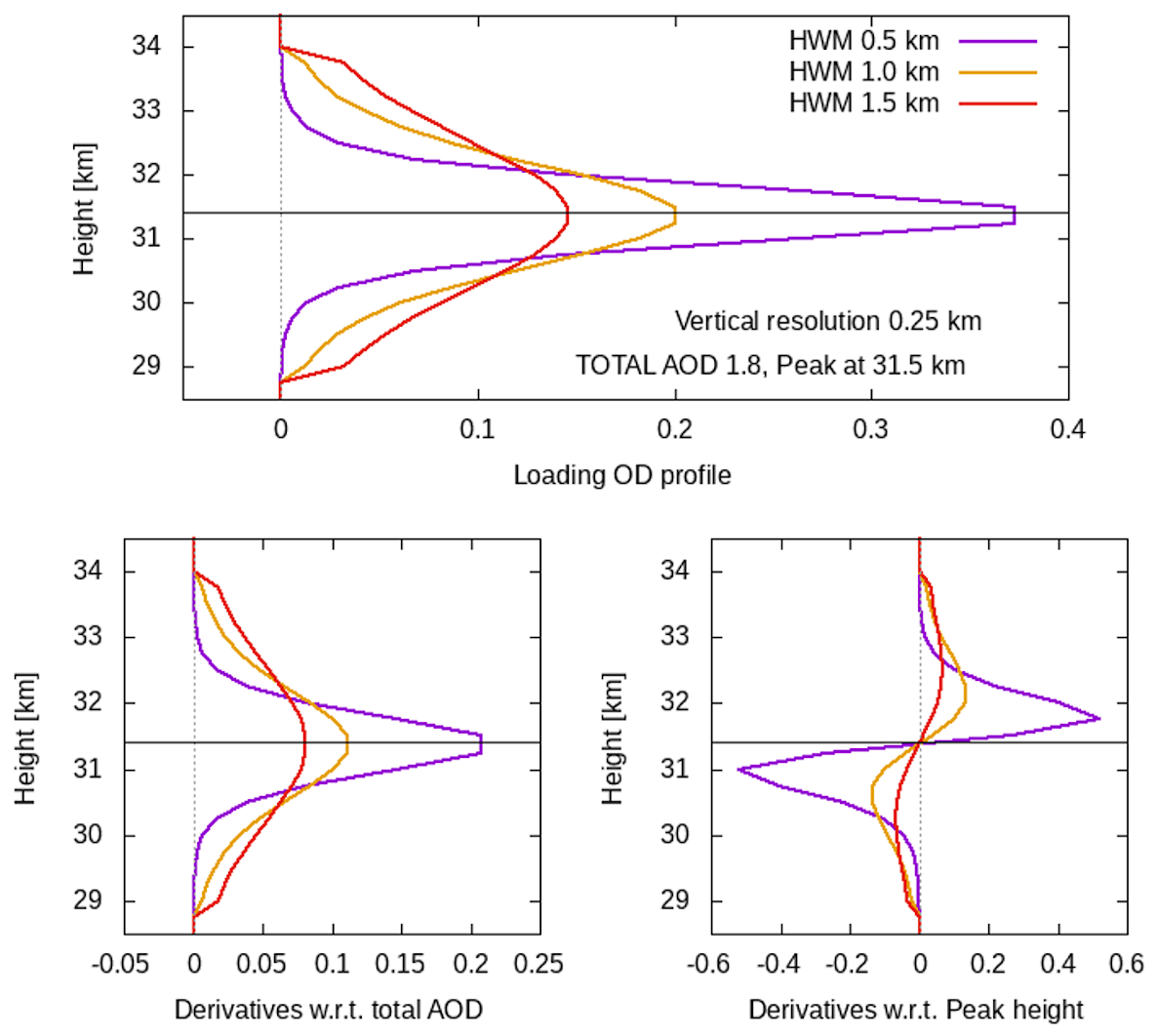
Figure A1 (Upper panel) Pseudo-Gaussian aerosol plume profiles over the 28–35 km altitude range, for three different Half-Width at Half-Maximum (HWHM) values as indicated. (Lower panels) Profile derivatives with respect to AOD and peak height.

The treatment here follows that in Spurr and Christi (2014). We use the same pseudo-Gaussian plume parameterization scheme for aerosols and for the other trace gases (SO₂, O₃); the exposition here is given just for aerosols but applies equally to the two trace species. The aerosol plume is characterized by three parameters $\left\{A_{\mathrm{0}},z_{\mathrm{p}},h_{\mathrm{w}}\right\}$: A₀ is the plume total optical depth at a fixed reference wavelength λ_ref (312 nm), z_p is the plume peak height in [km], and h_w is the HWHM in [km] of the plume distribution. We retrieve the first two of these parameters; the state vector is $\mathit{x}=\left\{A_{\mathrm{0}},z_{\mathrm{p}}\right\}$. The pseudo-Gaussian plume is the aerosol optical thickness profile at 312 nm, given by:

$$\begin{array}{}\text{(A1)}& \mathit{\tau }\left(z\right)=\mathrm{\Omega }{\displaystyle \frac{\exp [-f(z-z_{\mathrm{p}}\left)\right]}{{\left[\mathrm{1}+\exp [-f(z-z_{\mathrm{p}}\left)\right]\right]}^{\mathrm{2}}}}.\end{array}$$

Here, z is the altitude, z_p is the peak height (“PKH”), Ω is a normalization constant related to total stratospheric aerosol optical thickness (“AOD”) A₀, and f is an exponential constant related to the HWHM parameter h_w through $f{h}_{\mathrm{w}}=\ln \left[\mathrm{3}+\mathrm{2}\sqrt{\mathrm{2}}\right]$. At peak height z=z_p, the loading is $\mathit{\tau }\left(z_{\mathrm{p}}\right)=\frac{\mathrm{1}}{\mathrm{4}}\mathrm{\Omega }$.

We assume that the plume lies between two limiting heights z_b and z_t. Integrating the profile between these limits yields the total AOD:

$$\begin{array}{}\text{(A2)}& {\displaystyle }{A}_{\mathrm{0}}={\int }_{z_{\mathrm{b}}}^{z_{\mathrm{t}}}\mathit{\tau }\left(z\right)\mathrm{d}z=\mathrm{\Omega }\mathrm{\Gamma };\mathrm{\Gamma }={\displaystyle \frac{\left(Y_{\mathrm{b}}-Y_{\mathrm{t}}\right)}{\left(\mathrm{1}+Y_{\mathrm{b}}\right)\left(\mathrm{1}+Y_{\mathrm{t}}\right)}};\text{(A3)}& {\displaystyle }{Y}_{\mathrm{b}}=\exp \left[-f\left(z_{\mathrm{b}}-z_{\mathrm{p}}\right)\right];Y_{\mathrm{t}}=\exp \left[-f\left(z_{\mathrm{t}}-z_{\mathrm{p}}\right)\right].\end{array}$$

For a discretization of the atmosphere into vertical layers {z_n}, $n=\mathrm{0},\mathrm{1},\mathrm{\dots }{N}_{\mathrm{L}}$, where N_L is the total number of layers, the loading profile will be given by:

$$\begin{array}{}\text{(A4)}& {\displaystyle }{L}_n={\int }_{z_n}^{z_{n-\mathrm{1}}}\mathit{\tau }\left(z\right)\mathrm{d}z={\displaystyle \frac{A_{\mathrm{0}}}{\mathrm{\Gamma }}}{\mathrm{\Gamma }}_n;.\text{(A5)}& {\displaystyle }{\mathrm{\Gamma }}_n={\displaystyle \frac{\left(Y_n-Y_{n-\mathrm{1}}\right)}{\left(\mathrm{1}+Y_n\right)\left(\mathrm{1}+Y_{n-\mathrm{1}}\right)}};Y_n=\exp \left[-f\left(z_n-z_{\mathrm{p}}\right)\right].\end{array}$$

Here we have used Eq. (A2) to show that each layer amount L_n is directly proportional to A₀. The forward model radiative transfer calculation using VLIDORT requires Jacobians with respect to A₀ and z_p, plus h_w if the latter is to be included in the retrieval or is to be considered as a model parameter error in the retrieval. We require partial derivatives of the loading profile with respect to these parameters. Explicit differentiation of Eq. (A4) gives:

$$\begin{array}{}\text{(A6)}& \begin{array}{rl}& {\displaystyle \frac{\partial L_n}{\partial A_{\mathrm{0}}}}={\displaystyle \frac{{\mathrm{\Gamma }}_n}{\mathrm{\Gamma }}};{\displaystyle \frac{\partial L_n}{\partial z_{\mathrm{p}}}}={\displaystyle \frac{\mathrm{1}}{\mathrm{\Gamma }}}\left[{\displaystyle \frac{\partial {\mathrm{\Gamma }}_n}{\partial z_{\mathrm{p}}}}-L_n{\displaystyle \frac{\partial \mathrm{\Gamma }}{\partial z_{\mathrm{p}}}}\right];\\ & {\displaystyle \frac{\partial L_n}{\partial h_{\mathrm{w}}}}={\displaystyle \frac{\mathrm{1}}{\mathrm{\Gamma }}}\left[{\displaystyle \frac{\partial {\mathrm{\Gamma }}_n}{\partial h_{\mathrm{w}}}}-L_n{\displaystyle \frac{\partial \mathrm{\Gamma }}{\partial h_{\mathrm{w}}}}\right].\end{array}\end{array}$$

The A₀ derivative is trivial. Derivatives with respect to z_p are harder to establish; after some algebra, we find the auxiliary derivatives of Γ and Γ_n through:

$$\begin{array}{}\text{(A7)}& \begin{array}{rl}& {\displaystyle \frac{\partial {\mathrm{\Gamma }}_n}{\partial z_{\mathrm{p}}}}=f{\mathrm{\Gamma }}_n{\displaystyle \frac{\left(\mathrm{1}-Y_n{Y}_{n-\mathrm{1}}\right)}{\left(\mathrm{1}+Y_n\right)\left(\mathrm{1}+Y_{n-\mathrm{1}}\right)}};\\ & {\displaystyle \frac{\partial \mathrm{\Gamma }}{\partial z_{\mathrm{p}}}}=f\mathrm{\Gamma }{\displaystyle \frac{\left(\mathrm{1}-Y_{\mathrm{b}}{Y}_{\mathrm{t}}\right)}{\left(\mathrm{1}+Y_{\mathrm{b}}\right)\left(\mathrm{1}+Y_{\mathrm{t}}\right)}}.\end{array}\end{array}$$

Similarly, the auxiliary derivative Γ_n with respect to h_w is given by:

$$\begin{array}{}\text{(A8)}& \begin{array}{rl}{\displaystyle \frac{\partial {\mathrm{\Gamma }}_n}{\partial h_{\mathrm{w}}}}& =-{\displaystyle \frac{C}{f^{\mathrm{2}}}}{\mathrm{\Gamma }}_n\left[z_{\mathrm{p}}-{\displaystyle \frac{\left(z_n{Y}_n-z_{n-\mathrm{1}}{Y}_{n-\mathrm{1}}\right)}{\left(Y_n-Y_{n-\mathrm{1}}\right)}}\right.\\ & \left.+{\displaystyle \frac{\left(z_n-z_{\mathrm{p}}\right)Y_n}{\left(\mathrm{1}+Y_n\right)}}+{\displaystyle \frac{\left(z_{n-\mathrm{1}}-z_{\mathrm{p}}\right)Y_{n-\mathrm{1}}}{\left(\mathrm{1}+Y_{n-\mathrm{1}}\right)}}\right].\end{array}\end{array}$$

A similar expression holds for the derivative of Γ with respect to h_w, but with Y_b and z_b replacing Y_n and z_n, and Y_t and z_t replacing with Y_n−1 and z_n−1. In Eq. (A8), the constant $C=\ln \left[\mathrm{3}+\sqrt{\mathrm{8}}\right]$.

Figure A1 (top panel) illustrates three typical pseudo-Gaussian plumes, with total AOD A₀=1.81, peak height z_p=31.5 km and three different values of h_w as indicated. The lower panels show the partial derivatives with respect to A₀ and z_p.

Treatment of the SO₂ trace gas profiles is similar. Plume parameters are the total column ${\mathrm{\Omega }}_{{\mathrm{SO}}_{\mathrm{2}}}$ in Dobson Units [DU], and the aerosol parameters z_p and h_w, when the plumes are positioned together and have the same shape. In this case, derivatives of the SO₂ plume profile with respect to z_p and h_w will then have exactly the same form as the expressions in Eqs. (A6) to (A8).

Appendix B: VLIDORT and the forward model

For radiance simulations, it is necessary to construct an input set of total optical properties (optical thickness values, single-scattering albedos, spherical-function expansion coefficients, scattering matrices) for VLIDORT. In addition, for calculations of associated Jacobians with respect to aerosol retrieval parameters, VLIDORT requires an additional set of linearized total optical property inputs. Determination of VLIDORT optical property inputs is discussed in this Appendix. VLIDORT is a discrete-ordinate polarized radiative transfer (RT) model in wide use in the remote sensing community. Single scattering in VLIDORT is treated accurately for line-of-sight and solar paths allowing for the Earth's curvature, while the multiple-scatter field is determined through plane-parallel scattering along with the pseudo-spherical approximation (solar beam attenuation for a curved atmosphere). The great advantage using VLIDORT lies in its ability to return not just the backscattered Stokes-vector radiation field, but also analytically-derived Jacobians of this field with respect to any atmospheric or surface property.

To cover all possible retrieval trials discussed in this work and planned sequel papers, we require VLIDORT to calculate Jacobians with respect to the three aerosol parameters $\left\{A_{\mathrm{0}},z_{\mathrm{p}},h_{\mathrm{w}}\right\}$, the single SO₂ parameter $\left\{{\mathrm{\Omega }}_{{\mathrm{SO}}_{\mathrm{2}}}\right\}$ and the three O₃ parameters $\left\{{\mathrm{\Omega }}_{{\mathrm{O}}_{\mathrm{3}}},z_{\mathrm{p},{\mathrm{O}}_{\mathrm{3}}},h_{\mathrm{w},{\mathrm{O}}_{\mathrm{3}}}\right\}$.

In VLIDORT, the atmosphere is taken as a series of optically uniform layers. Without loss of generality, the standard set of input optical properties (IOPs) is $\left\{{\mathrm{\Delta }}_n,{\mathit{\omega }}_n,{\mathbf{B}}_{n\mathrm{l}}\right\},n=\mathrm{1}$,...N_L, where Δ_n is the layer optical depth for extinction in layer n, ω_n the total single scattering albedo in that layer, and B_nl is a 4×4 matrix of spherical-function expansion coefficients that are used to develop the total scattering and phase matrices. [Scattering matrices can be specified in advance for the single-scattering calculations, as an alternative to developing them from sets of expansion coefficients]. For Jacobians, VLIDORT also requires the set of linearized IOPs $\left\{V_{nq},U_{nq},Z_{n\mathrm{l}q}\right\},n=\mathrm{1}$, ... N_L defined as the double-normalized partial derivatives of the IOPs with respect to Jacobian parameter ξ_q. In other words:

$$\begin{array}{}\text{(B1)}& V_{nq}={\displaystyle \frac{{\mathit{\xi }}_q}{{\mathrm{\Delta }}_n}}{\displaystyle \frac{\partial {\mathrm{\Delta }}_n}{\partial {\mathit{\xi }}_q}};U_{nq}={\displaystyle \frac{{\mathit{\xi }}_q}{{\mathit{\omega }}_n}}{\displaystyle \frac{\partial {\mathit{\omega }}_n}{\partial {\mathit{\xi }}_q}};Z_{n\mathrm{l}q}={\displaystyle \frac{{\mathit{\xi }}_q}{{\mathbf{B}}_{n\mathrm{l}}}}{\displaystyle \frac{\partial {\mathbf{B}}_{n\mathrm{l}}}{\partial {\mathit{\xi }}_q}}.\end{array}$$

Here, we determine these IOPs and associated parameter derivatives for the present application.

If the trace gas absorption optical thickness is G_n(λ) in layer n, the Rayleigh scattering optical thickness R_n(λ), and the aerosol extinction optical thickness E_n(λ) at wavelength λ, then the IOPs in that layer are:

$$\begin{array}{}\text{(B2a)}& {\mathrm{\Delta }}_n\left(\mathit{\lambda }\right)=G_n\left(\mathit{\lambda }\right)+R_n\left(\mathit{\lambda }\right)+E_n\left(\mathit{\lambda }\right);\end{array}$$

$$\begin{array}{}\text{(B2b)}& {\mathit{\omega }}_n\left(\mathit{\lambda }\right)={\displaystyle \frac{R_n\left(\mathit{\lambda }\right)+a\left(\mathit{\lambda }\right)E_n\left(\mathit{\lambda }\right)}{{\mathrm{\Delta }}_n\left(\mathit{\lambda }\right)}};\end{array}$$

$$\begin{array}{}\text{(B2c)}& {\mathbf{B}}_{n\mathrm{l}}\left(\mathit{\lambda }\right)={\displaystyle \frac{R_n\left(\mathit{\lambda }\right){\mathbf{B}}_{\mathrm{l}}^{\left(\mathrm{Ray}\right)}\left(\mathit{\lambda }\right)+a\left(\mathit{\lambda }\right)E_n\left(\mathit{\lambda }\right){\mathbf{B}}_{\mathrm{l}}^{\left(\mathrm{Aer}\right)}\left(\mathit{\lambda }\right)}{R_n\left(\mathit{\lambda }\right)+a\left(\mathit{\lambda }\right)E_n\left(\mathit{\lambda }\right)}}.\end{array}$$

Here a(λ) is the aerosol single scatter albedo, with $B_{\mathrm{l}}^{\left(\mathrm{Ray}\right)}$ and $B_{\mathrm{l}}^{\left(\mathrm{Aer}\right)}$ the coefficient matrices for Rayleigh and aerosol scattering respectively.

Now the aerosol extinction optical thickness E_n(λ) is related to the aerosol loading profile {L_n} at reference wavelength λ₀ through:

$$\begin{array}{}\text{(B3)}& E_n\left(\mathit{\lambda }\right)=r\left(\mathit{\lambda }\right)L_n={\displaystyle \frac{\mathit{ϵ}\left(\mathit{\lambda }\right)}{\mathit{ϵ}\left({\mathit{\lambda }}_{\mathrm{0}}\right)}}{L}_n.\end{array}$$

Here, ϵ(λ) is the coefficient for aerosol extinction at the wavelength of interest, with ϵ(λ₀) the extinction coefficient at reference wavelength λ₀, with r(λ) the ratio of these two quantities.

Similarly, the trace gas absorption term (with SO₂ included) is

$$\begin{array}{}\text{(B4)}& G_n\left(\mathit{\lambda }\right)={\mathit{\sigma }}_{n,{\mathrm{O}}_{\mathrm{3}}}\left(\mathit{\lambda }\right)L_{n,{\mathrm{O}}_{\mathrm{3}}}+{\mathit{\sigma }}_{n,{\mathrm{SO}}_{\mathrm{2}}}\left(\mathit{\lambda }\right)L_{n,{\mathrm{SO}}_{\mathrm{2}}};\end{array}$$

Here, $\left\{L_{n,{\mathrm{O}}_{\mathrm{3}}}\right\}$ and $\left\{L_{n,{\mathrm{SO}}_{\mathrm{2}}}\right\}$ are trace gas loading profiles, with absorption cross-sections denoted by ${\mathit{\sigma }}_{n,{\mathrm{O}}_{\mathrm{3}}}\left(\mathit{\lambda }\right)$ and ${\mathit{\sigma }}_{n,{\mathrm{SO}}_{\mathrm{2}}}\left(\mathit{\lambda }\right)$.

Given the aerosol loading profile {L_n} and gas profiles $\left\{L_{n,{\mathrm{O}}_{\mathrm{3}}}\right\}\left\{L_{n,{\mathrm{SO}}_{\mathrm{2}}}\right\}$, we are now in a position to derive the linearized optical properties in Eq. (B1) through explicit chain-rule differentiation of the results in Eqs. (B2)–(B4) with respect to any of the three aerosol parameters $\left\{A_{\mathrm{0}},z_{\mathrm{p}},h_{\mathrm{w}}\right\}$, the SO₂ parameter $\left\{{\mathrm{\Omega }}_{{\mathrm{SO}}_{\mathrm{2}}}\right\}$ or the three O₃ parameters $\left\{{\mathrm{\Omega }}_{{\mathrm{O}}_{\mathrm{3}}},z_{\mathrm{p},{\mathrm{O}}_{\mathrm{3}}},h_{\mathrm{w},{\mathrm{O}}_{\mathrm{3}}}\right\}$.

Dealing first with the aerosol profile {L_n}, and using the symbol ξ to indicate any one of the parameters $\left\{A_{\mathrm{0}},z_{\mathrm{p}},h_{\mathrm{w}}\right\}$, we find that:

$$\begin{array}{}\text{(B5a)}& {\displaystyle \frac{\partial {\mathrm{\Delta }}_n\left(\mathit{\lambda }\right)}{\partial \mathit{\xi }}}=r\left(\mathit{\lambda }\right){\displaystyle \frac{\partial L_n}{\partial \mathit{\xi }}};\text{(B5b)}& {\displaystyle \frac{\partial {\mathit{\omega }}_n\left(\mathit{\lambda }\right)}{\partial \mathit{\xi }}}=r\left(\mathit{\lambda }\right){\displaystyle \frac{\partial L_n}{\partial \mathit{\xi }}}\left[{\displaystyle \frac{a\left(\mathit{\lambda }\right)-{\mathit{\omega }}_n\left(\mathit{\lambda }\right)}{{\mathrm{\Delta }}_n\left(\mathit{\lambda }\right)}}\right];\text{(B5c)}& {\displaystyle \frac{\partial {\mathbf{B}}_{n\mathrm{l}}\left(\mathit{\lambda }\right)}{\partial \mathit{\xi }}}=a\left(\mathit{\lambda }\right)r\left(\mathit{\lambda }\right){\displaystyle \frac{\partial L_n}{\partial \mathit{\xi }}}\left[{\displaystyle \frac{{\mathbf{B}}_{n\mathrm{l}}^{\left(\mathrm{Aer}\right)}\left(\mathit{\lambda }\right)-{\mathbf{B}}_{n\mathrm{l}}\left(\mathit{\lambda }\right)}{R_n\left(\mathit{\lambda }\right)+a\left(\mathit{\lambda }\right)E_n\left(\mathit{\lambda }\right)}}\right].\end{array}$$

Dealing next with the O₃ profile $\left\{L_{n,{\mathrm{O}}_{\mathrm{3}}}\right\}$ and setting ${\mathit{\xi }}_{{\mathrm{O}}_{\mathrm{3}}}$ to any of the three O₃ parameters $\left\{{\mathrm{\Omega }}_{{\mathrm{O}}_{\mathrm{3}}},z_{p,{\mathrm{O}}_{\mathrm{3}}},h_{\mathrm{w},{\mathrm{O}}_{\mathrm{3}}}\right\}$, we have:

$$\begin{array}{}\text{(B6a)}& {\displaystyle \frac{\partial {\mathrm{\Delta }}_n\left(\mathit{\lambda }\right)}{\partial {\mathit{\xi }}_{{\mathrm{O}}_{\mathrm{3}}}}}={\mathit{\sigma }}_{n,{\mathrm{O}}_{\mathrm{3}}}\left(\mathit{\lambda }\right){\displaystyle \frac{\partial L_{n,{\mathrm{O}}_{\mathrm{3}}}}{\partial {\mathit{\xi }}_{{\mathrm{O}}_{\mathrm{3}}}}};\text{(B6b)}& {\displaystyle \frac{\partial {\mathit{\omega }}_n\left(\mathit{\lambda }\right)}{\partial {\mathit{\xi }}_{{\mathrm{O}}_{\mathrm{3}}}}}=-{\displaystyle \frac{{\mathit{\omega }}_n\left(\mathit{\lambda }\right)}{{\mathrm{\Delta }}_n\left(\mathit{\lambda }\right)}}{\displaystyle \frac{\partial {\mathrm{\Delta }}_n\left(\mathit{\lambda }\right)}{\partial {\mathit{\xi }}_{O\mathrm{3}}}};\text{(B6c)}& {\displaystyle \frac{\partial {\mathbf{B}}_{n\mathrm{l}}\left(\mathit{\lambda }\right)}{\partial {\mathit{\xi }}_{{\mathrm{O}}_{\mathrm{3}}}}}=\mathrm{0}.\end{array}$$

Note that these ozone derivatives are only present for the parameterized part of the profile; outside this range they are zero.

The situation with SO₂ is a little more complicated. For the SO₂ loading parameter ${\mathrm{\Omega }}_{{\mathrm{SO}}_{\mathrm{2}}}$, the derivatives are of the same form as those in Eq. (B6):

$$\begin{array}{}\text{(B7)}& \begin{array}{rl}& {\displaystyle \frac{\partial {\mathrm{\Delta }}_n\left(\mathit{\lambda }\right)}{\partial {\mathrm{\Omega }}_{{\mathrm{SO}}_{\mathrm{2}}}}}={\mathit{\sigma }}_{n,{\mathrm{SO}}_{\mathrm{2}}}\left(\mathit{\lambda }\right){\displaystyle \frac{\partial L_{n,{\mathrm{SO}}_{\mathrm{2}}}}{\partial {\mathrm{\Omega }}_{{\mathrm{SO}}_{\mathrm{2}}}}};\\ & {\displaystyle \frac{\partial {\mathit{\omega }}_n\left(\mathit{\lambda }\right)}{\partial {\mathrm{\Omega }}_{{\mathrm{SO}}_{\mathrm{2}}}}}=-{\displaystyle \frac{{\mathit{\omega }}_n\left(\mathit{\lambda }\right)}{{\mathrm{\Delta }}_n\left(\mathit{\lambda }\right)}}{\displaystyle \frac{\partial {\mathrm{\Delta }}_n\left(\mathit{\lambda }\right)}{\partial {\mathrm{\Omega }}_{{\mathrm{SO}}_{\mathrm{2}}}}};{\displaystyle \frac{\partial {\mathbf{B}}_{n\mathrm{l}}\left(\mathit{\lambda }\right)}{\partial {\mathrm{\Omega }}_{{\mathrm{SO}}_{\mathrm{2}}}}}=\mathrm{0}.\end{array}\end{array}$$

If the SO₂ plume is coincident with the aerosol plume, then there will be additional dependencies on the parameters {z_p,h_w}. Thus, we now have (in place of Eq. B5):

$$\begin{array}{}\text{(B8a)}& {\displaystyle \frac{\partial {\mathrm{\Delta }}_n\left(\mathit{\lambda }\right)}{\partial z_{\mathrm{p}}}}=r\left(\mathit{\lambda }\right){\displaystyle \frac{\partial L_n}{\partial z_{\mathrm{p}}}}+{\mathit{\sigma }}_{n,{\mathrm{SO}}_{\mathrm{2}}}\left(\mathit{\lambda }\right){\displaystyle \frac{\partial L_{n,{\mathrm{SO}}_{\mathrm{2}}}}{\partial z_{\mathrm{p}}}};\text{(B8b)}& {\displaystyle \frac{\partial {\mathit{\omega }}_n\left(\mathit{\lambda }\right)}{\partial z_{\mathrm{p}}}}={\displaystyle \frac{\mathrm{1}}{{\mathrm{\Delta }}_n\left(\mathit{\lambda }\right)}}\left[a\left(\mathit{\lambda }\right)r\left(\mathit{\lambda }\right){\displaystyle \frac{\partial L_n}{\partial z_{\mathrm{p}}}}-{\mathit{\omega }}_n\left(\mathit{\lambda }\right){\displaystyle \frac{\partial {\mathrm{\Delta }}_n\left(\mathit{\lambda }\right)}{\partial z_{\mathrm{p}}}}\right];\text{(B8c)}& {\displaystyle \frac{\partial {\mathbf{B}}_{n\mathrm{l}}\left(\mathit{\lambda }\right)}{\partial z_{\mathrm{p}}}}=a\left(\mathit{\lambda }\right)r\left(\mathit{\lambda }\right){\displaystyle \frac{\partial L_n}{\partial z_{\mathrm{p}}}}\left[{\displaystyle \frac{{\mathbf{B}}_{n\mathrm{l}}^{\left(\mathrm{Aer}\right)}\left(\mathit{\lambda }\right)-{\mathbf{B}}_{n\mathrm{l}}\left(\mathit{\lambda }\right)}{R_n\left(\mathit{\lambda }\right)+a\left(\mathit{\lambda }\right)E_n\left(\mathit{\lambda }\right)}}\right].\end{array}$$

This establishes the necessary optical inputs for VLIDORT to return simulated radiances and Jacobians for our retrieval trials. More details on optical property setups for VLIDORT may be found in the review literature (Spurr and Christi, 2019).

Appendix C: Determination of cloud screening index (CSI) threshold

To identify Hunga aerosol plume pixels and reduce interference with tropospheric clouds, we use a Cloud Screening Index (CSI), which is defined as a TROPOMI radiance ratio at a specific wavelength below 300 nm. The CSI wavelength and threshold were determined empirically. Radiance-ratio maps were generated at 0.5 nm intervals between 280 and 330 nm and examined (see Video Supplement S1). We found that short UV1 wavelengths fail to fully capture the Hunga plume, while longer UV2 wavelengths are affected by tropospheric clouds more than by Hunga aerosols (Fig. 2–4). Based on this analysis, radiance ratios at 296, 297, and 298 nm were selected as candidates for the CSI representative wavelength, since they minimized interference with tropospheric clouds while retaining good sensitivity to the Hunga volcanic aerosols. Figure C1 shows retrieved Hunga AOD maps filtered using the CSI at the candidate wavelengths (296, 297, and 298 nm) with CSI thresholds set at 1.05 and 1.1. Areas marked with black circles indicate regions influenced by tropospheric clouds. The threshold of 1.05 was found to be too low to effectively filter out tropospheric clouds at representative wavelengths. When the threshold was increased to 1.1, filtering at 297 and 298 nm still left some tropospheric cloud pixels, whereas filtering at 296 nm screened out most tropospheric clouds and captured most of the Hunga aerosol plume pixels (see Fig. 3). Therefore, the radiance ratio at 296 nm was selected as the CSI wavelength, with the associated threshold set to be 1.1.

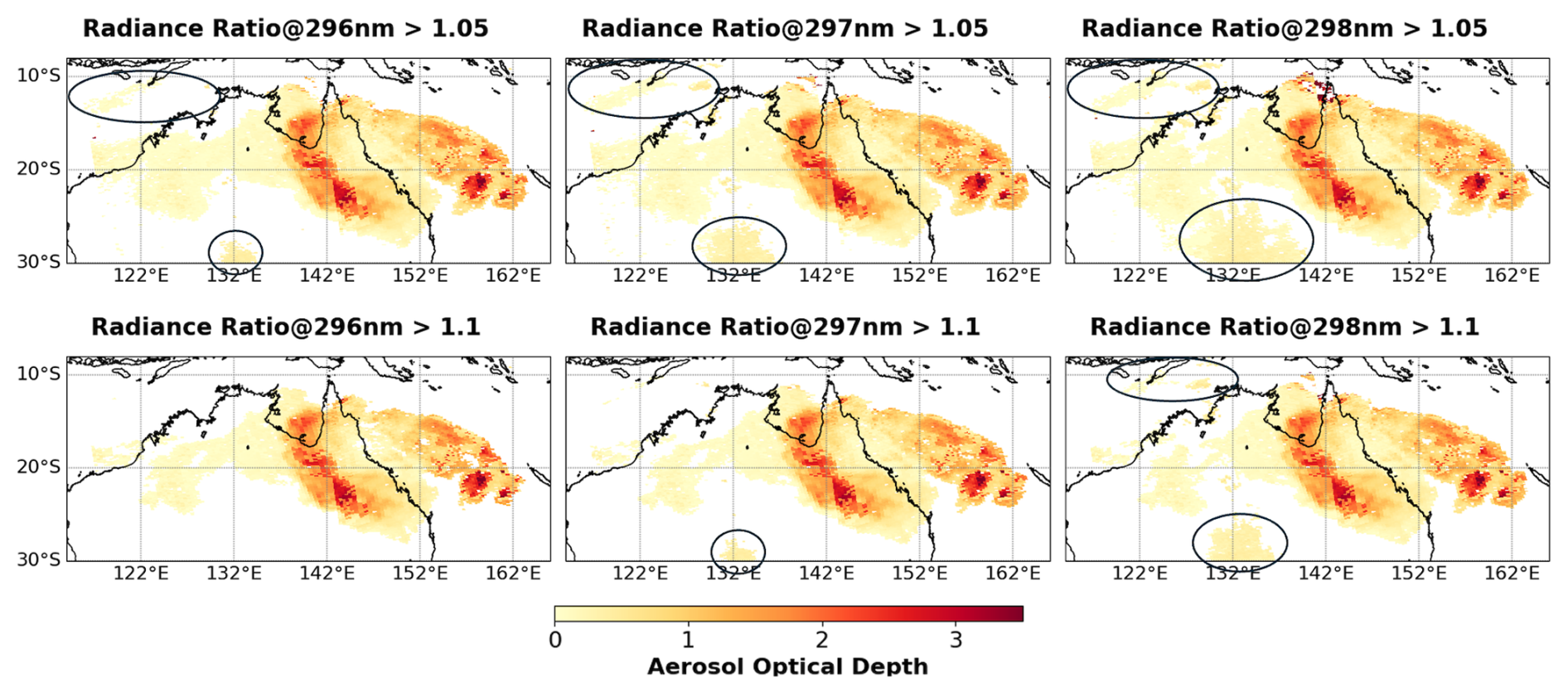
Figure C1 Hunga-retrieved AOD maps generated by filtering pixels based on radiance ratio thresholds (1.05 and 1.1) at three candidate CSI wavelengths of 296, 297, and 298 nm. Black circles indicate areas mainly influenced by tropospheric clouds.

Appendix D: NASA Goddard trajectory calculation of Hunga aerosol transport

The “ftraj” trajectory model from NASA's Goddard Space Flight Center Atmospheric Chemistry and Dynamics Laboratory uses a fourth-order Runge–Kutta integration scheme to track parcels isentropically, with optional diabatic adjustments (Schoeberl and Sparling, 1995). The model is driven with winds at 0.25° horizontal resolution and spaced every 6 h, from the Goddard Earth Observing System (GEOS) forward-processing system produced by the NASA Global Modeling and Assimilation Office (GMAO).

Figure D1b shows several trajectories calculated using the “ftraj” model. Parcels are started from nadir locations above the eruption point at different heights. In full accordance with the wind field, the tropospheric part of the volcanic plume at altitudes less than 17 km slowly drifts eastward, while the stratospheric part at altitudes higher than 17 km quickly moves westward.

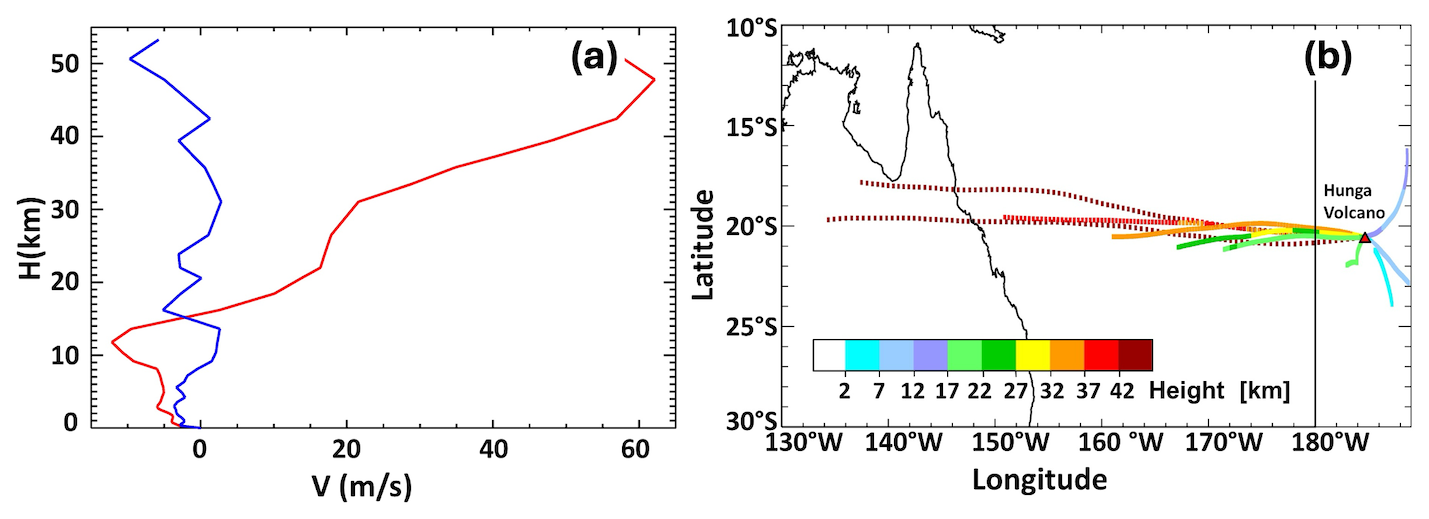
Figure D1 (a) Wind vertical profile near the Hunga volcano at the time of the eruption. The blue curve shows the speed of the meridional wind, the red curve the speed of the zonal wind. Clearly the meridional wind is weak at all altitudes, while the easterly winds increase with altitude. (b) Forward trajectories of air parcels that start from a location directly above the Hunga volcano at different heights, followed through 24 h using MERRA-2 reanalysis winds. The dotted lines represent parcels originating at altitudes exceeding 42 km.

Appendix E: Hunga aerosol retrieval from NOAA-20 OMPS-NP measurements

The NOAA-20 OMPS Nadir Profiler (OMPS-NP) provides backscattered ultraviolet (BUV) radiance spectra in the nadir viewing direction with a higher SNR, but a lower spectral resolution (FWHM ∼ 1 nm) than correspondingly for TROPOMI in the UV1 and UV2 spectral regions. Given the high SNR and spectral coverage of OMPS-NP, we conducted independent retrievals of AOD and aerosol layer height (z_p) within the Hunga plume. Figure E1 shows (left) the radiance ratio map (CSI at 296 nm) and (right) spectral radiance ratios along the Hunga plume orbit (o21577), referenced to a background orbit (o21575) on 17 January 2022. The enhancements of radiance ratios are consistent with the TROPOMI radiance ratio patterns presented in Fig. 1. The clear enhancement of OMPS-NP radiance ratios within the Hunga plume and the high SNR of OMPS-NP indicate that OMPS-NP data are sensitive enough to retrieve AOD and z_p. The same forward model inputs as described in Sect. 3 (e.g., corrected ozone profiles from M2-SCREAM and aerosol microphysical properties) were used in the OMPS-NP retrievals. Since spectral SNR values are required to construct the measurement and forward-model error covariance matrix S_ϵ (as noted in Sect. 3.3) and considering the noteworthy stray light rejection characteristics of the OMPS-NP instrument, the spectral SNR of OMPS-NP was assumed to be five times higher than the TROPOMI UV1 SNR.

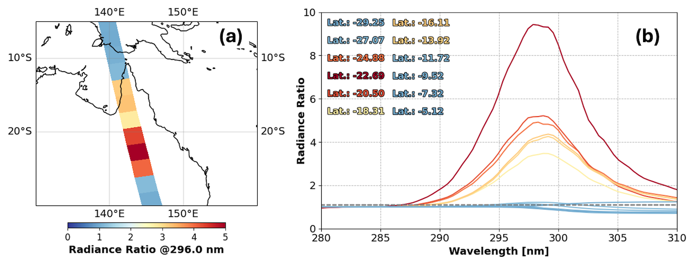
Figure E1 (a) OMPS-NP CSI map (radiance ratio at 296 nm) for the plume orbit (o21575) on 17 January 2022. (b) OMPS-NP spectral radiance ratios (280–310 nm) along the plume orbit (along-track: 35–46; Latitudes: 29.25 to 5.12° S) on 17 January 2022. Same color scale is applied to both plots. Spectral radiance ratios were derived from the ratio between the plume orbit (o21577) and the background orbit (o21575).

Figure E2 shows the retrieved AOD and z_p maps from OMPS-NP and TROPOMI along with their absolute and percentage differences. Both retrievals were performed assuming n_r=1.47. Smaller TROPOMI pixels were aggregated within OMPS-NP pixels, and to ensure a reasonable comparison, we excluded cases where the number of TROPOMI Hunga pixels with CSI > 1.1 was less than 20 % of the total number of collocated pixels. Retrieved AOD and z_p values are compared in Table E1 for OMPS-NP pixels 37 to 42. As shown in Fig. E2, the spatial distributions of z_p and AOD from OMPS-NP and aggregated TROPOMI pixels show good agreement. OMPS-NP z_p values are slightly lower than those of TROPOMI with an absolute difference (OMPS-NP minus TROPOMI) of 0.25 ± 0.15 km, with an averaged absolute percentage difference of ∼ 0.8 %, indicating excellent consistency in z_p retrievals between the two sensors. However, OMPS-NP AOD values are approximately ∼ 20 % higher than those from TROPOMI (0.24 ± 0.17). This result suggests that the higher SNR of OMPS-NP better capture enhanced aerosol signals, while TROPOMI still retrieves z_p values comparable to OMSP-NP.

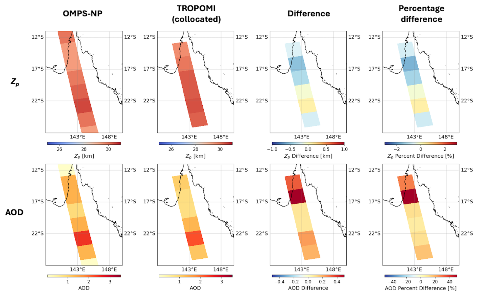
Figure E2 (Upper row) Aerosol peak height (z_p) maps retrieved from OMPS-NP and TROPOMI measurements assuming n_r=1.47, along with absolute and percentage differences between the two retrievals. (Lower row) Same as upper panel, but for the AOD. TROPOMI z_p and AOD values were collocated to match each OMPS-NP along-track location.

Table E1 Comparison of retrieved Hunga AOD and Aerosol Peak Height (z_p) between NOAA-20 OMPS-NP and TROPOMI, for selected along-track OMPS locations from 37 to 42.

Appendix F: Simulation of relative humidity and sulfate weight percent based on NASA Goddard Earth Observing System Chemistry Climate Model (GEOS CCM)

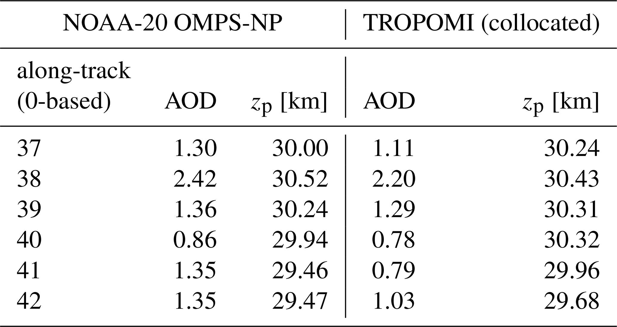
To quantify the relative humidity and percentage of sulfuric acid (sulfate) by mass in the Hunga aerosol solutions, we used a version of the GEOS Chemistry Climate Model (GEOS CCM) with the Community Aerosol and Radiation Model for Atmospheres (CARMA) similar to Case et al. (2023). This version of GEOS CCM: (1) calculates the oxidation of volcanic sulfur dioxide by online oxidant species and (2) includes a detailed, size-resolved treatment of aerosol microphysics including diagnosing the amount of water vapor that condenses on hygroscopic aerosols. This model was designed to simulate large volcanic eruptions and has been validated and used in multiple studies of stratospheric volcanic injections (Case et al., 2023, 2024; Zhu et al., 2025). We initialized this model with 0.5 Tg of SO₂ based on Carn et al. (2022), and consistent with the results of this study, water vapor such that the model retained about 150 Tg within the Hunga plume, as observed by the Microwave Limb Sounder (MLS). Figure F1 shows a zonal maximum of relative humidity and the associated percentage of sulfate by mass simulated by the model. In CARMA, the sulfate weight percentage is calculated following the method of Tabazadeh et al. (1997). Within the Hunga Plume itself, relative humidity values are as high as 60 % resulting in a sulfate weight percent as low as 40 %.

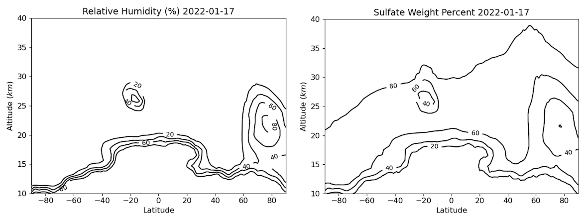
Figure F1 (Left) Zonal maximum relative humidity on 17 January 2022 in NASA GEOS CCM CARMA model. (Right) Sulfate (sulfuric acid) weight percentage of total aerosol mass associated with zonal maximum relative humidity.