Global spectroscopic survey of cloud thermodynamic phase at high spatial resolution, 2005–2015

The distribution of ice, liquid, and mixed phase clouds is important for Earth's planetary radiation budget, impacting cloud optical properties, evolution, and solar reflectivity. Most remote orbital thermodynamic phase measurements observe kilometer scales and are insensitive to mixed phases. This under-constrains important processes with outsize radiative forcing impact, such as spatial partitioning in mixed phase clouds. To date, the fine spatial structure of cloud phase has not been measured at global scales. Imaging spectroscopy of reflected solar energy from 1.4 to 1.8 µm can address this gap: it directly measures ice and water absorption, a robust indicator of cloud top thermodynamic phase, with spatial resolution of tens to hundreds of meters. We report the first such global high spatial resolution survey based on data from 2005 to 2015 acquired by the Hyperion imaging spectrometer onboard NASA's Earth Observer 1 (EO-1) spacecraft. Seasonal and latitudinal distributions corroborate observations by the Atmospheric Infrared Sounder (AIRS). For extratropical cloud systems, just 25 % of variance observed at GCM grid scales of 100 km was related to irreducible measurement error, while 75 % was explained by spatial correlations possible at finer resolutions.

1 Introduction

The distribution of ice, liquid, and mixed phase clouds is important for Earth's climate and planetary radiation budget (Chylek et al., 2006; Martins et al., 2011). Cloud thermodynamic phase affects radiative forcing by modulating absorption of incoming solar radiation, particle evolution, and lifetime (Ehrlich et al., 2008; Tan and Storelvmo, 2016). Previous satellite observational studies have shown that clouds are shifting poleward in the northern and southern hemispheric extratropical storm tracks (Bender et al., 2012; Marvel et al., 2015; Norris et al., 2016). Within these shifting storm tracks, climate model experiments with forcing from increased CO₂ have shown losses of cloud ice phase and gains of cloud liquid phase (Ceppi and Hartmann, 2015; McCoy et al., 2015). This makes cloud phase an important property for accurate and continuous monitoring. Moreover, recent studies indicate that spatial partitioning of ice and liquid particles within clouds has outsized influence on climate, affecting global climate model (GCM) predictions of future warming by over 1 ^∘C (Tan et al., 2016). However, current observing systems cannot reduce this uncertainty; they are unable to resolve differences at critical sub-100 m scales or are insensitive to mixed phase clouds altogether.

Imaging reflectance spectroscopy from 1.4 to 1.8 µm could address this gap. Prior work used this spectral interval to measure cloud phase based on the optical absorption properties of liquid and ice (Pilewskie and Twomey, 1987). The fraction of the total path absorption due to liquid (the liquid thickness fraction, or LTF) had high sensitivity to pure and mixed phases (Thompson et al., 2016). Liquid and ice show highly diagnostic absorption shapes which are robust to potential confounding effects such as surface reflectance, observation geometry, and mismatch in particle modeling assumptions. Remote imaging spectrometers measure these spectra from cloud tops at millions of spatial locations, resolving cloud phase at scales of tens of meters (Thompson et al., 2016). This could constrain characteristic spatial lengths of these processes. However, global spectroscopic datasets have not yet been analyzed in this way.

Here we report a global spectroscopic survey of cloud phase from 2005 to 2015 based on data from the Hyperion imaging spectrometer instrument onboard NASA's Earth Observer 1 (EO-1) spacecraft. Hyperion also provides two novel contributions beyond prior records. First, its full spectrum fitting discriminates mixed phases by directly measuring the relative contributions of physical cloud top liquid and ice absorption. Second, Hyperion measures phase at horizontal scales of 30 m. These properties allow the first rigorous characterization of the spatial scales governing cloud top thermodynamic phase. The article first describes our estimation method, and reports seasonal and latitudinal changes of cloud thermodynamic phase. We then compare these distributions to measurements by NASA's Atmospheric Infrared Sounder (AIRS) (Kahn et al., 2014). Finally, we show the spatial scaling properties of both extratropical and tropical cloud populations. The study lays the groundwork for future orbital imaging spectrometers (Mouroulis et al., 2016) that can monitor cloud characteristics when cloud cover precludes their primary mission. Imaging spectroscopy investigations typically treat clouds as contamination, when in fact cloudy data can be exploited to dramatically increase these instruments' useful data yield.

2 Cloud phase estimation

2.1 Method

The Hyperion imaging spectrometer operated on the sun synchronous EO-1 spacecraft for over a decade prior to decommissioning in 2017. Hyperion measured reflected solar energy from approximately 400 to 2450 nm with approximately 10 nm spectral sampling. It performed targeted acquisitions for specific regions of interest, with occasional pointing off nadir. Most targets were on land, with a high concentration in the midlatitude Northern Hemisphere. There was sparser coverage of extreme latitudes and oceans, but several island targets offered a view into cloud systems over ocean (Fig. 1). Many targets of interest were revisited multiple times during the mission. Each targeted acquisition had a ground sampling distance of approximately 30 m over a cross-track width of approximately 7.5 km, and a typical along-track distance of approximately 120 km. The Jet Propulsion Laboratory (JPL) Hyperion archive included most normal science acquisitions from 2005 through 2015, with over 4.8×10⁴ scenes and 3.7×10¹⁰ distinct spectra.

The archive was stored as standard calibrated unorthorectified data. We first applied the cloud phase retrieval algorithm of Thompson et al. (2016), validated in the prior work by coincident remote and in situ aircraft measurements. We defined the TOA reflectance, ρ:

$$\begin{array}{}\text{(1)}& \mathit{\rho }\left(\mathit{\lambda }\right)=\mathit{\pi }L\left(\mathit{\lambda }\right)/\left(F\left(\mathit{\lambda }\right)\cos \left({\mathit{\theta }}_{\mathrm{0}}\right)\right),\end{array}$$

where λ was the wavelength, L was the wavelength-dependent radiance at sensor, F was the extraterrestrial solar irradiance, and θ₀ was the solar zenith angle. Over short intervals we modeled ρ by a linear continuum with an offset a and slope b, attenuated by one or more Beer–Lambert absorbers j. Each absorber had a bulk absorption coefficient k_j and a nonnegative thickness u_j:

$$\begin{array}{}\text{(2)}& \mathit{\rho }\left(\mathit{\lambda }\right)=\left(a+b\mathit{\lambda }\right)\exp \left[-\sum _j{k}_j\left(\mathit{\lambda }\right)u_j\right]\mathrm{for}{u}_j\ge \mathrm{0}.\end{array}$$

We modeled three absorbers: atmospheric water vapor (j=1), liquid water (j=2), and ice (j=3). As in Thompson et al. (2015, 2016) we applied a logarithmic transformation resulting in a nonnegative least-squares problem (Lawson and Hanson, 1974):

$$\begin{array}{ll}{\displaystyle }& {\displaystyle }-\log \left(\mathit{\rho }\left(\mathit{\lambda }\right)\right)\approx l+m\mathit{\lambda }+\sum _j{k}_j\left(\mathit{\lambda }\right)u_j\\ \text{(3)}& {\displaystyle }& {\displaystyle }\mathrm{for}l\ge \mathrm{0},u_j\ge \mathrm{0}\forall j.\end{array}$$

Here m permitted a log-linear continuum. We represented this to the solver as two nonnegative coefficients for upward and downward slopes, one of which would evaluate to zero. The nonnegative least-squares solution provided stable global solutions without sensitivity to initialization.

Figure 1 The JPL Hyperion archive comprised over 45 000 scenes, represented here by red dots. The majority were over land. A green arrow indicates the Ross Island acquisition of Fig. 2.

We calculated the H₂O vapor absorption coefficients using the HITRAN 2012 line list (Rothman et al., 2013) via the Oxford Reference Forward Model (Dudhia, 2014). We initialized the vapor abundance using a band ratio retrieval as in Thompson et al. (2015) and used this to calculate an “effective” absorption coefficient of band-aggregated vapor lines for use in the least-squares retrieval. Other atmospheric gases did not significantly impact the shape of vapor absorption features. We calculated liquid and ice absorption coefficients using the complex index of refraction measured by Kou et al. (1993). These bulk absorption spectra were molecular properties of H₂O, independent of particle size and scattering – a common practice for shortwave infrared observations of clouds (Kokhanovsky, 2004). Combined with a free continuum, they fit the observed spectra of opaque clouds over short spectral intervals without precise knowledge of particle properties (Thompson et al., 2016).

In summary, following Eq. (3) we modeled the entire interval from 1.4 to 1.8 µm with five free parameters: a continuum offset l; a slope, represented by a single degree of freedom in the variables m and n; and the vapor, ice, and liquid thicknesses u_j. These thicknesses represented the length of the optical path through an equivalent homogeneous volume, as in the equivalent water thickness (Gao and Goetz, 1995). As in previous work, we wrote the absorption path length u₂ as the equivalent water thickness due to liquid in millimeters, EWT_liquid. Similarly, u₃ was the equivalent water thickness due to ice, EWT_ice. We then defined the liquid thickness fraction as

$$\begin{array}{}\text{(4)}& \mathrm{LTF}={\displaystyle \frac{{\mathrm{EWT}}_{\mathrm{liquid}}}{{\mathrm{EWT}}_{\mathrm{liquid}}+{\mathrm{EWT}}_{\mathrm{ice}}}}.\end{array}$$

Prior in situ validation had demonstrated a robust relationship between the LTF and thermodynamic phase (Thompson et al., 2016). We emphasize that “thickness” referred to the absorption along the optical path; clouds were heterogeneous, so the LTF was not necessarily related to their vertical dimension. In opaque clouds the measurement would be most sensitive to the upper layers.

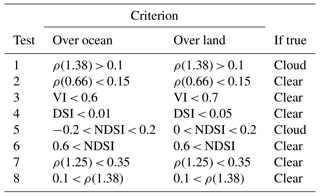
We calculated the LTF of locations flagged by the Hyperion cloud detection algorithm of Griffin et al. (2003). In the Griffin et al. approach, a decision tree of threshold tests sorted spectra into different cloud types (including low and high clouds) as well as different land cover types (including snow, open terrain surfaces, and vegetation). This favored opaque clouds and generally ignored ambiguous translucent clouds that would be difficult to distinguish from land. The Griffin et al. algorithm defined tests using the top-of-atmosphere (TOA) reflectance ρ and three intermediate quantities, the normalized difference snow index (NDSI), the desert sand index (DSI), and the vegetation index (VI):

$$\begin{array}{}\text{(5)}& {\displaystyle }& {\displaystyle }\mathrm{NDSI}=\left[\mathit{\rho }\left(\mathrm{0.55}\right)-\mathit{\rho }\left(\mathrm{1.65}\right)\right]/\left[\mathit{\rho }\left(\mathrm{0.55}\right)+\mathit{\rho }\left(\mathrm{1.65}\right)\right],\text{(6)}& {\displaystyle }& {\displaystyle }\mathrm{DSI}=\left[\mathit{\rho }\left(\mathrm{0.86}\right)-\mathit{\rho }\left(\mathrm{1.65}\right)\right]/\left[\mathit{\rho }\left(\mathrm{0.86}\right)+\mathit{\rho }\left(\mathrm{1.65}\right)\right],\text{(7)}& {\displaystyle }& {\displaystyle }\mathrm{VI}=\mathit{\rho }\left(\mathrm{0.66}\right)/\mathit{\rho }\left(\mathrm{0.86}\right).\end{array}$$

The method was originally formulated as a flowchart but was tantamount to an ordered sequence of tests (Table 1). It evaluated each spectrum independently, applying appropriate thresholds depending on whether the scene was over ocean or land. It ascribed a classification based on the first test that evaluated to true. Random manual validation of selected scenes demonstrated adequate performance, outside the brightest glacial scenes in Antarctica.

After calculating LTF maps over all cloud areas, we aggregated counts of liquid and ice clouds. LTF was a continuous-valued quantity so the maps revealed both pure and mixed phases. We binned LTF values in 10 % graduations but also calculated binary classification using a 50 % threshold. This facilitated comparisons with historical datasets of hard categorical classifications. We then analyzed zonal distributions, estimating confidence intervals with nonparametric bootstrap variance estimation (Wasserman, 2006) that resampled the dataset 10 000 times with replacement.

Table 1 Hyperion cloud detection algorithm (Griffin et al., 2003). We test each criterion in sequence, starting from the top, and ascribe a classification based on the first test that evaluates to true.

Evaluating the model fit to the spectrum demanded special care, since the global catalogue included many observing geometries, terrain surface types, and potential variability in instrument calibration over the decadal record. To account for this, we estimated the noise level independently for each integration timestep and each spectral channel. We used the common method of pairwise differences between spectra at neighboring locations (Boardman and Kruse, 2011). Since the spatial field was mostly uniform over small distances, these differences conservatively estimated the measurement noise σ in each channel. For n cross-track locations, we applied the nonparametric variance estimate of von Neumann (1941), reprised in Brown and Levine (2007):

$$\begin{array}{}\text{(8)}& {\widehat{\mathit{\sigma }}}^{\mathrm{2}}={\displaystyle \frac{\mathrm{1}}{\mathrm{2}(n-\mathrm{1})}}\sum _{i=\mathrm{1}}^{n-\mathrm{1}}{\left({\mathit{\rho }}_{i+\mathrm{1}}-{\mathit{\rho }}_i\right)}^{\mathrm{2}}.\end{array}$$

We then characterized the fit for each spectrum using the reduced χ² measure (Eldering et al., 2017), a statistical summary of the residual relative to the expected measurement errors. Specifically, it was the chi-squared score per degree of freedom, with χ²=1 equivalent to estimated measurement noise. This was more appropriate than a classical chi-squared test for our spectroscopic observations where errors could be correlated across adjacent wavelengths. For ℓ spectral channels, with measured TOA reflectance ρ and the model estimate $\widehat{\mathit{\rho }}$, the reduced χ² error was

$$\begin{array}{}\text{(9)}& {\mathit{\chi }}^{\mathrm{2}}={\displaystyle \frac{{\sum }_{\mathrm{\ell }}{\left(\mathit{\rho }-\widehat{\mathit{\rho }}\right)}^{\mathrm{2}}}{{\sum }_{\mathrm{\ell }}{\widehat{\mathit{\sigma }}}^{\mathrm{2}}}}.\end{array}$$

The summations ran over all ℓ spectral channels.

2.2 Results

The retrievals clearly revealed distinct cloud phases. Figure 2 shows an example sub-image drawn from a larger flightline. Figure 3 is the corresponding EWT_liquid and EWT_ice mapped to green and blue channels, respectively. LTF values in the mixed phase region range from 0.5 to 0.75, and values in ice areas are typically 0–0.2. Both regions were well-distinguished without significantly overlapping values, but also showed sub-kilometer interior spatial structure. Figure 4 shows normalized histograms of χ² scores for the entire scene, calculated independently for liquid and ice clouds. Fits were generally quite good, with χ² scores below the conservative noise estimate, χ²=1. In other words, the algorithm fit these cloud spectra to within the measurement accuracy, showing applicability of the Thompson et al. (2016) three absorber model o Hyperion data.

Figure 5 shows typical spectrum fits from locations in this sub-image, with mixed cloud and ice cloud. The top rows show the model fit to spectrum, confirming that the five-parameter model fit the 1.4–1.8 µm interval. The middle rows show transmittance due to each absorbing component in the model. The continuum component is not shown. The three absorbers together were sufficient to explain observed spectrum shapes. Finally, the bottom rows show residual error, which was again below the estimated measurement noise level.

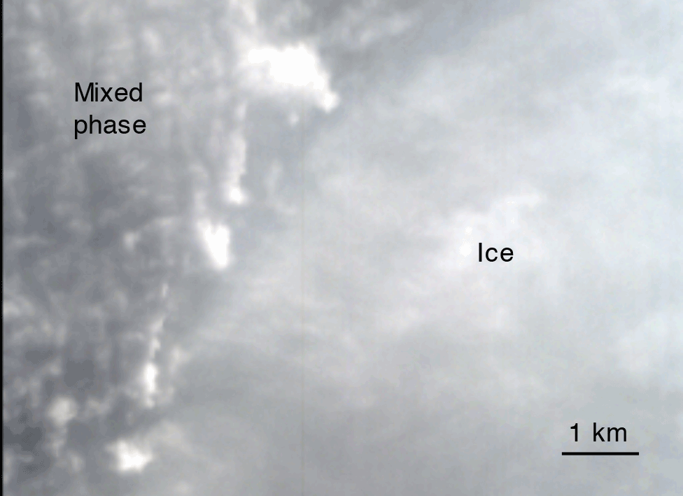
Figure 2 Typical fragment of a top-of-atmosphere reflectance image, drawn from Hyperion product ID EO1H2221282005350110KF over Ross Island, Antarctica, and displayed in visible red, green, and blue channels.

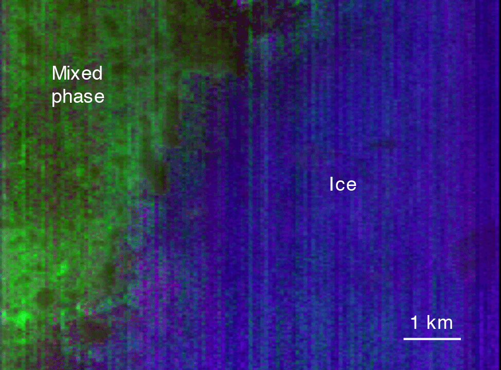
Figure 3 Thermodynamic phase map corresponding to Fig. 2, with green indicating equivalent liquid thickness and blue indicating equivalent ice thickness.

Figure 4 Normalized histogram of χ² spectrum fit scores for the entire scene of Figs. 2 and 3. Low χ² values indicate good fits; χ²=1 is a conservative estimate of measurement noise.

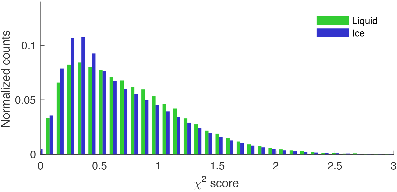
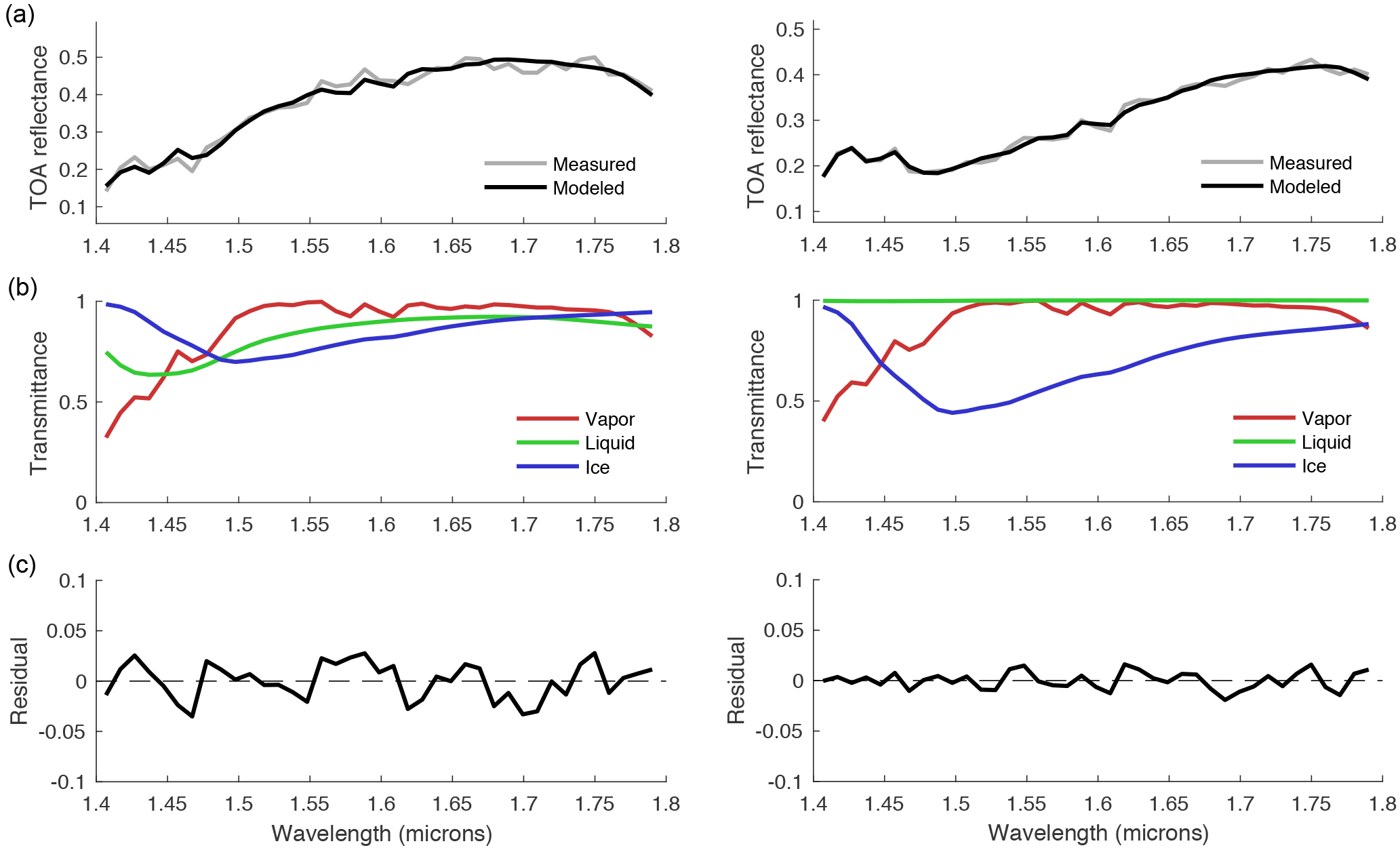
Figure 5 Spectrum fits from the region of mixed and ice cloud in Fig. 2. (a) Model fit to spectrum. (b) Transmittances for each absorber. (c) Residual error.

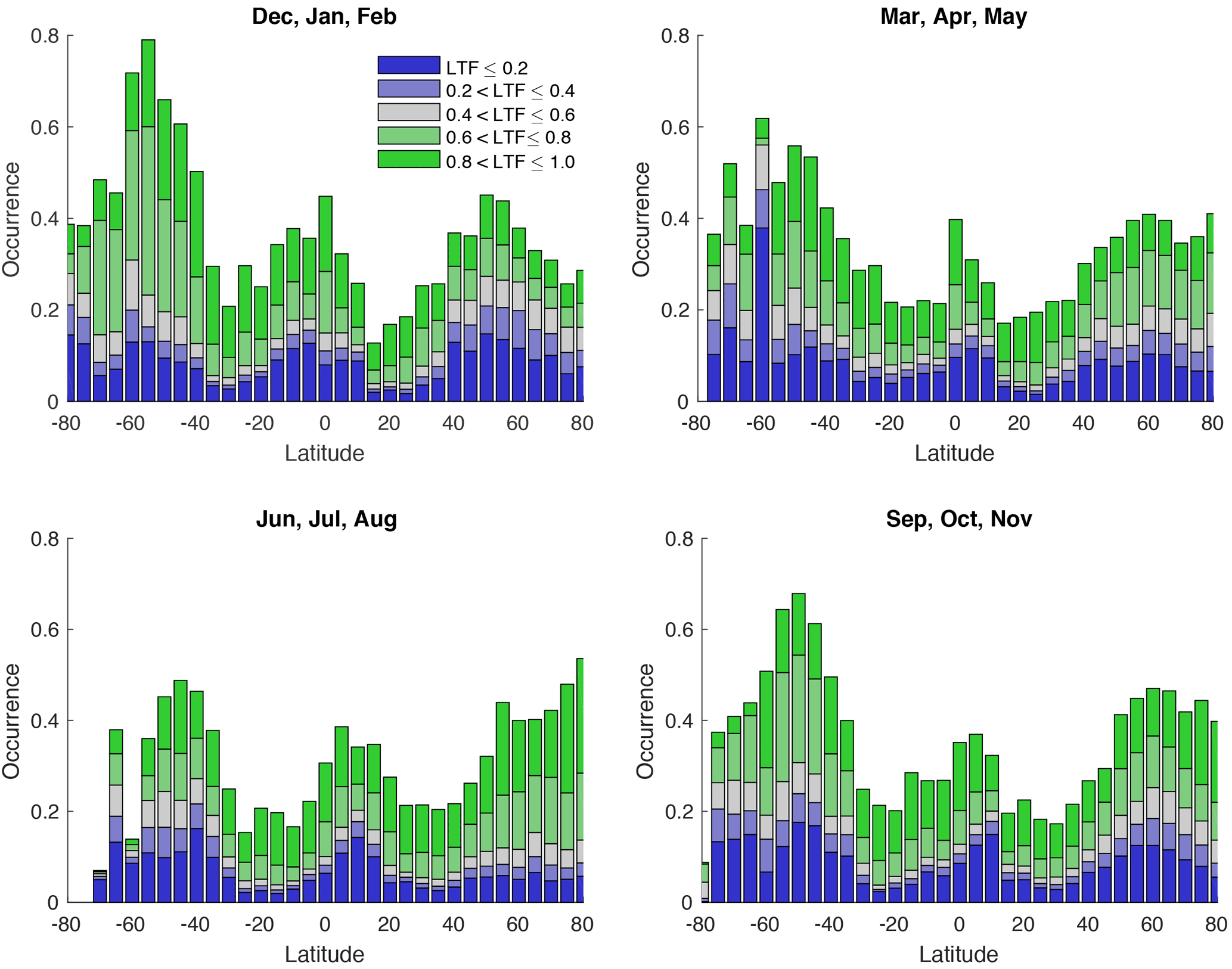
Figure 6 Zonal average cloud phase, partitioned by season, for all 10 years of observations. Sampling is nonuniform across latitudes; Sect. 3 quantifies uncertainty due to finite sample sizes.

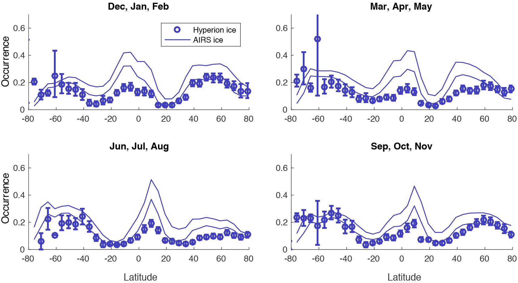
Figure 6 shows the entire distribution of mixed and pure phase clouds for all 10 years of observations and binned in 10^∘ increments, ranging from pure ice (LTF<0.2) to pure liquid (LTF>0.8). Note that Hyperion sampling is nonuniform across histogram bins, and Sect. 3 quantifies uncertainty for different latitudes. The dataset clearly resolved key features apparent in records from other sensors like MODIS and CALIPSO (Hirakata et al., 2014; Hu et al., 2010). A band of ice clouds peaked in the Intertropical Convergence Zone at approximately 5–10^∘ latitude, and other seasonally dependent maxima appeared at approximately 60 and −60^∘. The population associated with the LTF range from 0.6 to 0.8 was fairly large and possibly included some pure water pixels that were misclassified due to estimation noise. The mixed phase clouds were most numerous in the middle and extreme high latitudes and less abundant in the tropics. There was a general increase in the occurrence of liquid clouds at middle and high latitudes, with a strong asymmetry near the solstice: a seasonal peak in liquid cloud coverage for the summer months was apparent in both hemispheres.

3 AIRS comparison

3.1 Method

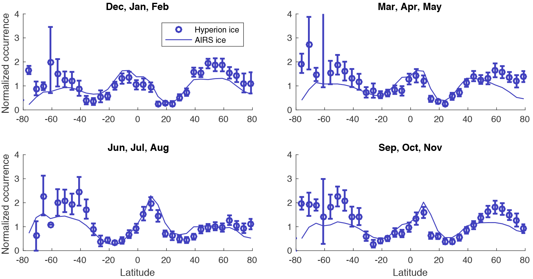
Next, we compared the resulting thermodynamic phase retrievals to a decadal dataset of cloud phase retrievals by the AIRS instrument (Pagano et al., 2003). This was a dramatically different measurement obtained from thermal infrared spectra with a coarse 13.5 km footprint rather than reflected solar energy at fine spatial resolution. Kahn et al. (2014) detail the algorithm, and Jin and Nasiri (2014) validate it using pixel-scale comparisons with CALIPSO data. We filtered clouds using an AIRS sensitivity threshold (effective cloud fraction, or ECF) of 0.1 and binned AIRS phases by latitude and season for direct comparison.

We anticipated several differences in the result. First, AIRS sampled uniformly over the Earth's surface while Hyperion imaged only during the day and favored land areas. We also expected differences in sensitivity; AIRS was far more sensitive to optically thin clouds, while the Hyperion analysis intentionally excluded thin clouds with a strict detection threshold. To help account for these differences, we normalized the relative cloud abundances of both instruments. We designated a reference latitude band from −60 to 60^∘ (the area of densest Hyperion coverage) to have a mean occurrence of unity and compared zonal changes relative to this standard.

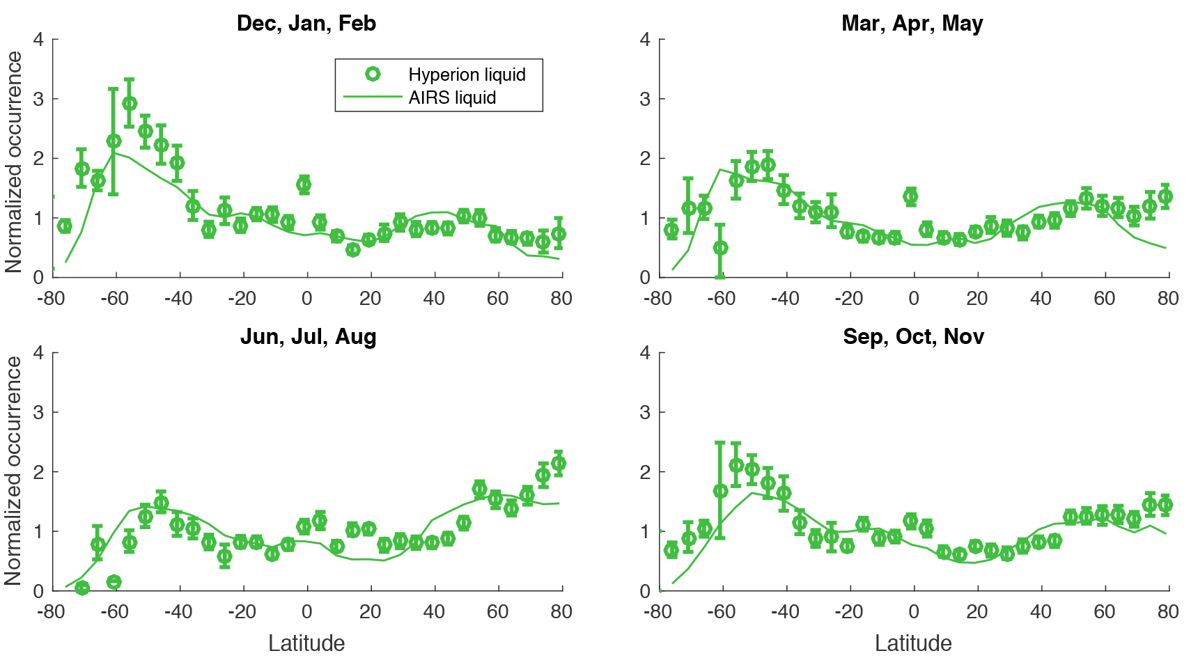
Figure 7 Comparison of Hyperion and AIRS cloud statistics, both normalized by the −60 to 60^∘ latitude range to account for differences in cloud mask cutoff thresholds. The 10-year seasonal observations are shown separately for the liquid phase. Here Hyperion uses a hard classification; i.e., liquid thickness fractions less than 0.5 are considered ice clouds. Error bars show 95 % confidence intervals calculated via nonparametric bootstrap estimation. The corresponding AIRS error bars would be far smaller due to the large number of samples, so we omit them for clarity.

Additionally, the AIRS algorithm classified ambiguous clouds as “unknown”. This population likely contained mixed phase clouds but also a large fraction of supercooled liquid clouds due to the current AIRS phase algorithm. The liquid tests are based on warm liquid water indices of refraction rather than the supercooled liquid indices of refraction (Rowe et al., 2013). Following from results of Jin and Nasiri (2014), we reassigned some of the unknown clouds to form 10 % of total ice and 60 % of total liquid. For liquid clouds, we defined a corrected occurrence L^′ in each latitude bin and took just 40 % of this to be from the original AIRS estimate L:

$$\begin{array}{}\text{(10)}& (\mathrm{1}-\mathrm{0.6})\sum L^{\prime }=\sum L,\end{array}$$

where summations ran over all latitude bins. This allowed a unique correction for each latitude bin, given as the product of its unknown cloud fraction U and a global multiplicative coefficient α:

$$\begin{array}{}\text{(11)}& L^{\prime }=L+\mathit{\alpha }U.\end{array}$$

Equations (6) and (7) gave

$$\begin{array}{}\text{(12)}& \mathit{\alpha }={\displaystyle \frac{\mathrm{0.6}\sum L}{(\mathrm{1}-\mathrm{0.6})\sum U}}.\end{array}$$

We defined a similar relation for ice cloud with a missing fraction of 0.1 rather than 0.6. Together, the two adjustments (magnitude normalization and reassignment of unknown clouds) accounted for known biases, which permitted a comparison of zonal gradients between the two instruments. While we expected some discrepancies due to differences in instruments and sampling, the comparison provided a useful check between two very different measurement techniques.

Figure 8 As in Fig. 7, for the ice phase.

3.2 Results

Figures 7 and 8 show liquid and ice cloud phase spatial distributions across latitudes, partitioned by season, for all 10 years of observations binned in 10^∘ increments. Error bars show 95 % confidence intervals for the mean. Thin lines indicate decadal averages derived from the AIRS dataset. Distributions from the two instruments generally agreed – particularly for ice, to which AIRS was very sensitive. Tropical ice clouds showed the best agreement, as in prior studies comparing AIRS and CALIPSO (Jin and Nasiri, 2014). Differences may be related to the much stronger sensitivity to thin ice cloud, coarse spatial resolution and near-global daily sampling, and ambiguity of the unknown category with respect to how many liquid, ice, and mixed phase clouds are contained within that categorization. Another potential contributor to the discrepancy is sensitivity to different altitudes in large or multilayer cloud systems. Multilayered clouds are abundant in tropical regions and midlatitude storm tracks. In cases where, for example, a translucent ice cloud overlays an optically thin liquid cloud, the two instruments would measure different thermodynamic phase. For reference, we place a non-normalized comparison of the two instrument datasets in Appendix A.

4 Spatial scale analysis

4.1 Method

We next characterized spatial scaling properties of the thermodynamic phase maps. A variogram (Garrigues et al., 2006) estimated the expected squared differences between LTF at any two locations x and x^′ in the map as a function v(d) of the lag distance d between the paired points. We used the classical estimator based on the sample variance at each lag distance:

$$\begin{array}{}\text{(13)}& v\left(d\right)={\displaystyle \frac{\mathrm{1}}{\mathrm{2}N\left(d\right)}}\sum _{\Vert x-x^{\prime }\Vert =d}{\left(\mathrm{LTF}\left(x\right)-\mathrm{LTF}\left(x^{\prime }\right)\right)}^{\mathrm{2}},\end{array}$$

where N(d) was the number of such points in the sample. The näive formulation involving calculations of all point pairs would have required over 10¹⁰ squared differences per scene, an intractable number. Instead, we calculated the same quantity efficiently in the Fourier domain using the method of Marcotte (1996), with a spatial mask to ensure that only cloud pixels influenced the calculation.

Table 2 Model parameters of tropical and extratropical clouds, for $v=a{d}^b+c$, with confidence bounds and R squared coefficients.

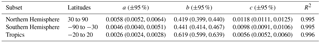
We fit the resulting variogram with a power law of the form $v\left(d\right)=a{d}^b+c$, subsampling the data to achieve log-constant point density and optimizing free parameters with the Levenberg–Marquardt method. We considered the hypothesis that tropical clouds would have different spatial scaling from extratropical clouds because of the dominant influence of convective versus baroclinic systems. To test this, we analyzed the scenes in three segments: a tropical band within 20^∘ of the Equator and extratropical scenes poleward of 30^∘ north and south latitudes. We used cloud fields larger than a 3 km cutoff, excluding variograms that evaluated to zero at shorter lag distances due to the lack of sufficient cloud pixels in the scene.

4.2 Results

Finally, Fig. 9 shows variograms over all years. Each data point corresponds to a lag distance for an aggregate variogram, so separation between the curves does not imply complete separation between populations. However, statistical analysis does reveal some significant differences in scaling properties. Table 2 shows the best-fitting coefficients for variance v in the liquid thickness fraction of tropical clouds, northern hemispheric extratropical clouds, and southern hemispheric extratropical clouds, as a function $v\left(d\right)=a{d}^b+c$ of distance d in kilometers. R² values indicate the power law is an excellent least-squares fit. Parenthesis indicate 95 % confidence intervals on the parameters.

We report scaling exponents in terms of variance; these could be translated to other conventions using structure functions or the power spectrum domain. Differences between the power law exponents for tropical and extratropical clouds were statistically significant. The extratropical scaling exponents of 0.42 and 0.44 are similar to, but slightly in excess of the classic Kolmogorov scaling of 1∕3 ($-\mathrm{5}/\mathrm{3}$ in the power spectral domain). The tropical scaling exponent of 0.62 is in excess of the classic Kolmogorov scaling of 1∕3 but is consistent with tropical cloud reflectance variability reported in Barker et al. (2017) and mid-tropospheric water vapor mixing ratio in the tropics from the AIRS instrument, e.g., Kahn et al. (2011). At finer spatial resolutions there is also evidence of scale breaks dependent on altitude. Consequently the scaling exponent is dependent on the length scale range calculated (Kahn et al., 2011).

Figure 9 Variogram for all clouds in the Hyperion dataset, showing the variance as a function of separation between points. The curve suggests a power law relationship. Dotted lines indicate 95 % confidence intervals on the coefficients.

The additive offset c defined the variance at zero distance, i.e., the irreducible measurement error for each spectrum. This implied a noise-equivalent change in liquid water fraction of approximately 7.5 % for tropical and 10–11 % for extratropical clouds. The addend and pre-factor coefficients differed significantly between extratropical and tropical clouds and to a much smaller degree between the two extratropical populations. All three populations were subject to Hyperion's biased sampling of ocean and land and of instrument noise conditions dominated by solar zenith angles. We would not ascribe differences between northern and southern hemispheres to cloud scaling since these discrepancies were small relative to their separation from the tropical model. In all cases, measurement error was a minor contributor to observed variance – most variability arose from spatially correlated structure. Outside the tropics, measurement error accounted for just 25 % of variance observed at GCM grid scales of 100 km. The remaining 75 % was therefore attributable to spatial structure at subgrid scales.

5 Conclusions

This study reports the first global high spatial resolution survey of cloud thermodynamic phase. The Hyperion imaging spectrometer provides two novel contributions beyond prior records. First, highly diagnostic spectral features permit accurate discrimination of mixed phase clouds. Second, horizontal scales down to 30 m capture the characteristic spatial scaling relationships of the thermodynamic phase field. Aggregate seasonal and latitudinal changes of cloud thermodynamic phase generally corroborate observations by other sensing modalities, such as those of AIRS. Variogram analysis reveals a noise-equivalent measurement error of 7.5–11 % in the liquid thickness fraction for different latitudinal zones. Spatial correlations follow a power law relationship with approximately 50 % measurable variance determined at length scales of 6 km. Significant spatial variability appears at scales far below the resolution of typical GCMs.

We note an important caveat to these results. The Hyperion datasets were spatially biased and strongly favored land mass over ocean. Insofar as the latitudinal distributions show asymmetries across northern and southern hemispheres, this may be related to the spatial distribution of land mass in the southern hemispheric midlatitude areas. Southern Hemisphere observations were often acquired over islands, which would exhibit a more oceanic influence on cloud cover.

Despite this qualification, the Hyperion results generally corroborate existing global datasets where there is overlap, a useful complement to instruments measuring cloud phase with polarization or thermal emission. They provide a “first of its kind” observational record at sub-kilometer scales. These scales are critical for advancing subgrid parameterizations in GCMs, including the Wegener–Bergeron–Findeisen timescale of the growth of ice crystals (Tan and Storelvmo, 2016) and numerous other temperature-dependent microphysical processes that control ice and liquid water partitioning (Ceppi et al., 2016), and for further extending the observational record to a new extreme of spatial resolution.

Appendix A: Non-normalized AIRS comparisons

Figures A1 and A2 show AIRS zonal averages for liquid and ice, respectively, with the correction of Jin and Nasiri (2014) but without normalization across latitudes. Thin lines indicate AIRS frequencies for ECF thresholds of 0.1 and 0.5. This indicates the sensitivity of the AIRS result to this choice. The absolute abundance of the ice phase shows the largest disparities. This is expected and accountable to very thin ice clouds to which AIRS is far more sensitive.

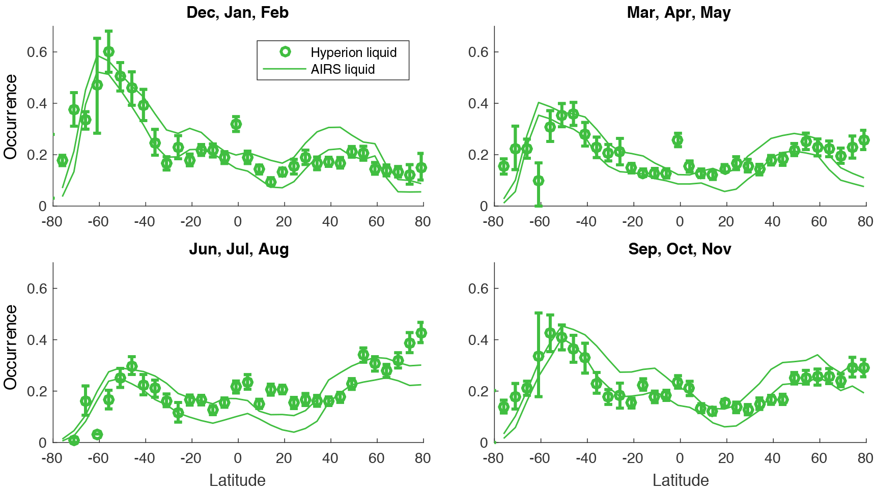
Figure A1 A comparison similar to Fig. 7 without normalization across latitudes. Two thin lines represent AIRS retrievals using the standard effective cloud fraction retrieval threshold of 0.5 and 0.1.

Figure A2 As in Fig. A1, for the ice phase.