Wave-optics uncertainty propagation and regression-based bias model in GNSS radio occultation bending angle retrievals

A new reference occultation processing system (rOPS) will include a Global Navigation Satellite System (GNSS) radio occultation (RO) retrieval chain with integrated uncertainty propagation. In this paper, we focus on wave-optics bending angle (BA) retrieval in the lower troposphere and introduce (1) an empirically estimated boundary layer bias (BLB) model then employed to reduce the systematic uncertainty of excess phases and bending angles in about the lowest 2 km of the troposphere and (2) the estimation of (residual) systematic uncertainties and their propagation together with random uncertainties from excess phase to bending angle profiles. Our BLB model describes the estimated bias of the excess phase transferred from the estimated bias of the bending angle, for which the model is built, informed by analyzing refractivity fluctuation statistics shown to induce such biases. The model is derived from regression analysis using a large ensemble of Constellation Observing System for Meteorology, Ionosphere, and Climate (COSMIC) RO observations and concurrent European Centre for Medium-Range Weather Forecasts (ECMWF) analysis fields. It is formulated in terms of predictors and adaptive functions (powers and cross products of predictors), where we use six main predictors derived from observations: impact altitude, latitude, bending angle and its standard deviation, canonical transform (CT) amplitude, and its fluctuation index. Based on an ensemble of test days, independent of the days of data used for the regression analysis to establish the BLB model, we find the model very effective for bias reduction and capable of reducing bending angle and corresponding refractivity biases by about a factor of 5. The estimated residual systematic uncertainty, after the BLB profile subtraction, is lower bounded by the uncertainty from the (indirect) use of ECMWF analysis fields but is significantly lower than the systematic uncertainty without BLB correction. The systematic and random uncertainties are propagated from excess phase to bending angle profiles, using a perturbation approach and the wave-optical method recently introduced by Gorbunov and Kirchengast (2015), starting with estimated excess phase uncertainties. The results are encouraging and this uncertainty propagation approach combined with BLB correction enables a robust reduction and quantification of the uncertainties of excess phases and bending angles in the lower troposphere.

1 Introduction

The bending angle (BA) and atmospheric profiles retrieval chain for Global Navigation Satellite System (GNSS) radio occultation (RO) data includes many steps involving linear and (moderately) nonlinear transformations, starting from excess phase and amplitude measurements (Gorbunov et al., 2006). Error or uncertainty propagation through the geometric optical part of the retrieval chain has been investigated in a series of theoretical and empirical studies (Kursinski et al., 1997; Syndergaard, 1999; Palmer et al., 2000; Rieder and Kirchengast, 2001; Kuo et al., 2004; Steiner and Kirchengast, 2005; Schreiner et al., 2007; Scherllin-Pirscher et al., 2011b; Scherllin-Pirscher et al., 2011a; Scherllin-Pirscher et al., 2017; Innerkofler et al., 2016; Schwarz et al., 2016; Schwarz et al., 2017a; Schwarz et al., 2017b; Li et al., 2016; Li et al., 2017).

The uncertainty propagation through the wave-optical bending angle retrieval block was investigated recently for large-scale (systematic) and small-scale (random) uncertainties by Gorbunov and Kirchengast (2015), including simulation results demonstrating random uncertainty propagation. Such wave-optical retrieval is essential in the lower troposphere (altitudes below 5 km), where the RO observations are subject to several specific uncertainties not present higher up in the atmosphere, including effects from low signal-to-noise ratio, multipath propagation, and super-refraction (Sokolovskiy, 2001, 2003; Xie et al., 2006; Ao, 2007; Xie et al., 2010; Sokolovskiy et al., 2010).

A thorough treatment of systematic uncertainty and its propagation from excess phase to bending angle in the lower troposphere, including the aim to correct for the known boundary layer bias (BLB) in standard lower troposphere RO retrievals, often termed the “negative refractivity bias” (Sokolovskiy et al., 2010; Gorbunov et al., 2015), is lacking so far. Also, the propagation of both estimated systematic and estimated random uncertainties through the wave-optical chain, complementary to the geometric-optical uncertainty propagation work of Schwarz et al. (2017a, b), has not been investigated and demonstrated yet. This study focuses on providing these missing investigations and on demonstrating BLB correction for a representative large ensemble of real RO data from the Constellation Observing System for Meteorology, Ionosphere, and Climate (COSMIC) mission as well as introducing a complete uncertainty propagation approach. The findings and algorithms obtained are used in the development of the new reference occultation processing system (rOPS) including an RO retrieval chain with integrated uncertainty propagation (Kirchengast et al., 2015, 2016a, b).

Our starting points for the BLB model construction are the approach based on refractivity fluctuations introduced by Gorbunov et al. (2015) and the recent study of RO systematic errors by Gorbunov (2014). Refractivity fluctuations constitute an external factor that results in a systematic shift in the signal phase due to its physical nature rather than any deficiency of the processing algorithm. Although this model cannot be looked at as a complete explanation of the bias, it serves as a convenient structural model that allows exposing probable candidates for the role of the objective characteristics of the signal received that may correlate with the bias. These characteristics will hereafter be referred to as predictors in the BLB model. In particular, it has already been shown by Gorbunov (2014) that the bending angle can serve as such a predictor. Further predictors and the complete BLB model setup based on a regression-modeling approach are described in this study.

This approach results in the BLB and (residual) systematic uncertainty model formulated in terms of tropospheric bending angles. In order to incorporate this uncertainty modeling into the RO retrieval chain with integrated uncertainty propagation, it needs to be transferred into the equivalent excess phase BLB and (residual) systematic uncertainty estimate. For its propagation, a perturbation approach or the approximation derived by Gorbunov and Kirchengast (2015) can be employed. In that paper we discussed the propagation of excess phase to bending angle uncertainty through the Fourier integral operator (FIO) used for the bending angle retrieval (Gorbunov and Lauritsen, 2004). This uncertainty propagation uses the stationary phase approximation, which allowed for the derivation of simple propagation formulae.

In order to now transform the bending angle uncertainty into the equivalent excess phase uncertainty, we use the inverse FIO, which was recently employed by Gorbunov (2016) for the retrieval of reflected rays from RO data. Specifically, the systematic uncertainty is evaluated for every RO event in the form of estimated profiles of bending angle BLB and (residual) systematic uncertainty. These estimates are then transformed into the equivalent BLB and (residual) systematic uncertainty of the excess phase, where they complement the estimated random and basic systematic uncertainty of the excess phase, which is available separately from the preceding step of excess phase processing (Innerkofler et al., 2016; Schwarz et al., 2017a, b). Both together are used as input to the wave-optical uncertainty propagation.

The paper is organized as follows. In Sect. 2 we describe the empirical BLB model, based on a regression analysis guided by the understanding that refractivity fluctuation statistics induce such biases, as well as a simple (residual) systematic uncertainty model for the BLB-corrected bending angles. Section 3 describes the wave-optical propagation of estimated systematic and random uncertainties from excess phase to bending angle for the methodology also recalling the key results needed from Gorbunov and Kirchengast (2015) and Gorbunov (2016). In Sect. 4 we discuss the results of the application of the BLB correction based on a large ensemble of COSMIC RO data from representative test days throughout the year 2008. Section 5 provides our conclusions.

2 Boundary layer bias (BLB) model of bending angle and its uncertainty

The BLB model is formulated to be capable of providing bending angle BLB profiles over the lower troposphere up to 5 km impact altitude, corresponding to about 4 km (mean-sea-level) altitude, with the primary bias effects occurring within the atmospheric boundary layer below about 2 km altitude. Here we describe its setup by first introducing the underlying refractivity fluctuations model (Sect. 2.1), which is then followed by the BLB model description (Sect. 2.2). The model is built as a regression model using adaptive functions based on predictors available for each RO event, including impact altitude, latitude, bending angle, BA standard deviation, canonical transform (CT) amplitude, and the CT amplitude fluctuation index as the main ones. The selection of the predictors is explained in Sect. 2.3 and their use in constructing the adaptive functions in Sect. 2.4.

Along with the description we illustrate the performance of the BLB model to quantify the boundary layer biases based on the predictors, underpinning that the BLB profiles obtained for individual RO events can be effectively used for BLB correction and lead to a significant reduction of systematic uncertainty. A simple model for the estimated residual systematic uncertainty after the BLB profile subtraction, which accounts for the residual bias and the uncertainty (indirectly) incurred from the use of ECMWF analysis profiles as regression reference, is described in Sect. 2.5.

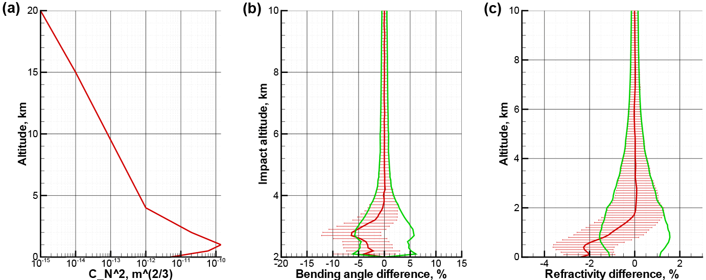
Figure 1 Deviation statistics induced by simulated refractivity fluctuations: refractivity structure constant $C_N^{\mathrm{2}}\left(z\right)$ profile (a) and associated difference statistics of ECMWF profiles with and without fluctuations superposed for bending angle as function of impact altitude (b) and refractivity as function of altitude (c), where mean difference (red), standard deviation (green), and the difference-ensemble spread (horizontal bars at vertical levels) are shown. COSMIC event geometry and concurrent ECMWF analysis fields from the 15th day of every month of year 2008 were used to produce the statistics.

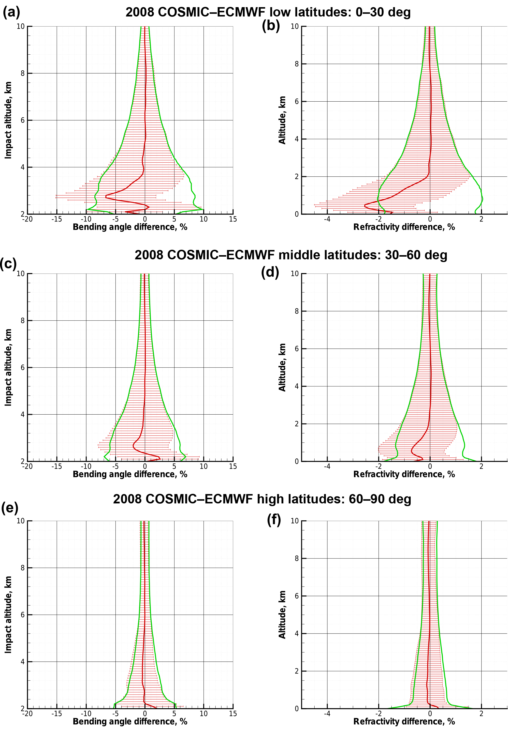
Figure 2 Deviation statistics obtained for real RO data: difference statistics of COSMIC profiles including real fluctuations relative to ECMWF profiles without fluctuations for bending angle as function of impact altitude (a, c, e) and refractivity as function of altitude (b, d, f), with the same style of panels as for the difference statistics in Fig. 1. Results for low latitudes (a, b), midlatitudes (c, d), and high latitudes (e, f) are shown for COSMIC events and concurrent ECMWF analysis fields from the 15th day of every month of year 2008.

2.1 Underlying model of refractivity fluctuations

In order to formulate our approach to the bending angle BLB in terms of the negative refractivity bias (Sokolovskiy et al., 2010), we use the fluctuation-based model introduced by Gorbunov et al. (2015). This model is used as a simple structural model that allows finding good candidates for the objective characteristics of the observed signals that correlate with the bias. Figure 1 shows an example profile of the refractivity structure constant $C_N^{\mathrm{2}}\left(z\right)$ and the corresponding relative difference statistics of an ensemble of bending angle and refractivity profiles. The latter were obtained by comparison of the modeled “truth” based on ECMWF refractivity fields, used as reference, and perturbed data based on the same ECMWF fields but with random refractivity fluctuations according to the $C_N^{\mathrm{2}}\left(z\right)$ profile superimposed. The $C_N^{\mathrm{2}}\left(z\right)$ profile was tuned to realistically represent BLB statistics of RO observations and the wave-optics propagator (WOP) package (Gorbunov, 2011) was used to realistically compute the bending angles.

It is visible in Fig. 1 that the refractivity fluctuations lead to a negative refractivity bias of up to about 2 % in the boundary layer and an associated negative BLB in bending angle of up to about 5 %, which is typical of biases seen in real RO data. Random differences (standard deviation) reach realistic values as well – about 1.5 % in refractivity and about 5 % in bending angle.

To put these simulation results into direct context with real data, Fig. 2 shows another set of difference statistics for bending angles and refractivities, from low latitudes to high latitudes, where we again used the modeled truth from ECMWF fields as reference but now to illustrate the differences of observed profiles from COSMIC. The COSMIC data were processed by the OCC (occultations) package for RO data processing, as described in Gorbunov et al. (2006). These results confirm that the refractivity fluctuations model, with corresponding settings, can reproduce the systematic and random error behavior of RO bending angles and refractivities in the boundary layer. A somewhat higher level of RMS deviations (standard deviation) seen for the COSMIC data, compared to Fig. 1, is likely caused by the fact that ECMWF fields themselves deviate from the real atmospheric state (see, e.g., the error modeling performed by Scherllin-Pirscher et al., 2011b, 2017).

Figure 3 presents a latitude–longitude map of the COSMIC–ECMWF refractivity differences at a height of 0.6 km in terms of systematic relative refractivity deviation. These results illustrate the regional variations in refractivity bias behavior and are similar to those presented in Xie et al. (2006, 2010) and Gorbunov (2014).

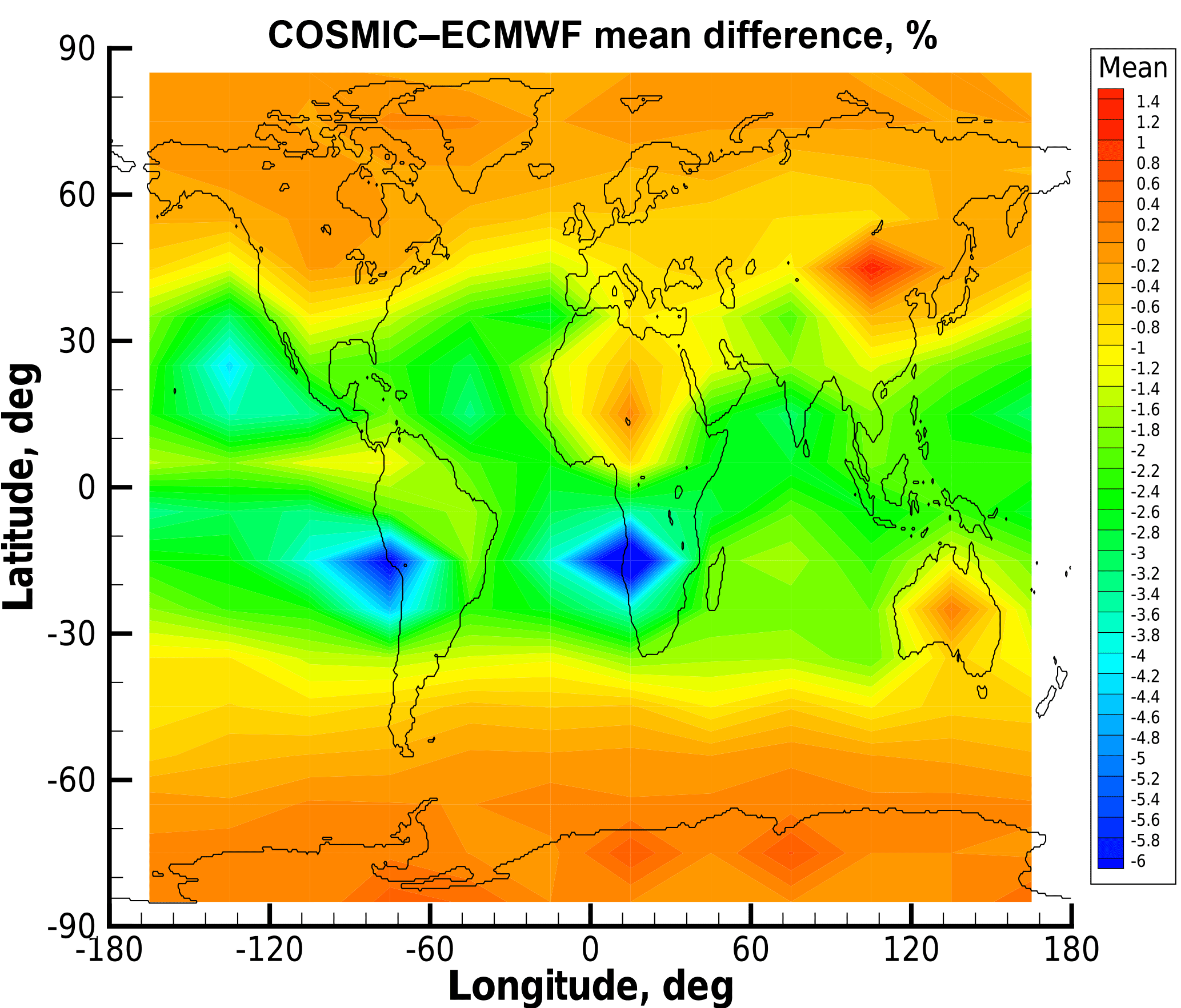
Figure 3 Deviation statistics obtained for real RO data: latitude–longitude map (10^∘ lat × 30^∘ long grid resolution) of difference statistics of COSMIC observations relative to ECMWF profiles without fluctuations for refractivity at an altitude of 0.6 km. Results are shown for COSMIC events and concurrent ECMWF analysis fields from the 1st, 11th, and 21st day of every month of year 2008.

Our further strategy of the bias correction consists in the following. We perform the numerical simulation of occultation events with superimposed fluctuations and analyze different objective characteristics of RO signals in order to find those that correlate with the simulated bias. These characteristics will be referred to as predictors. Using this set of predictors, we also compare the simulation results with the processing of real COSMIC observations. We assume that this will allow the formulation of a model for BLB correction, which will also effectively mitigate biases in the retrieved refractivity profiles and further-derived atmospheric profiles. We have to formulate the BLB model with a flexible functional behavior in order to reliably serve its purpose.

2.2 Bending angle BLB model from regression to adaptive functions

We model the BLB by a predictor-based empirical model that is flexible enough to capture the BLB behavior by suitable predictors under widely variable predictor value ranges for individual RO events. Because the dependence of the BLB model profiles from predictors is unknown a priori, we solve for this dependence in the form of the linear combination of a set of linear and nonlinear functions of the predictors. We refer to these functions as adaptive functions. The model estimate of the regression coefficients of the linear combination is based on the comparison of a large set of bending angle observations with a reference data set.

In this study, introducing a first reliable BLB model version, the observations are from the COSMIC mission and the reference data set consists of gridded fields of meteorological variables from ECMWF. The ECMWF data have their own systematic uncertainty, which is taken into account by letting these uncertainties flow into the estimated residual systematic uncertainty of bending angle profiles after BLB correction (Sect. 2.5).

The BLB model is formulated as follows. We used a set of COSMIC bending angle observations, including 24 representative days from year 2008. We adopted the 15th and 16th day of every month, amounting in total to about 54 000 RO events. We used the corresponding ECMWF fields as basis for obtaining the “true” reference bending angles. To this end, we employed the wave-optics propagator (Gorbunov, 2011) to generate the bending angle profiles from the ECMWF refractivity fields. We then performed a regression of the differences of observed and reference bending angles in the lower troposphere with respect to the chosen adaptive functions (Sect. 2.4). The adaptive functions are formulated in terms of predictors, which are evaluated from objective characteristics of every RO event, without using the reference data (Sect. 2.3). These ingredients allow for the derivation of regression coefficients, which upon their estimation complete the BLB model then ready to be applied based on predictors from a given RO event.

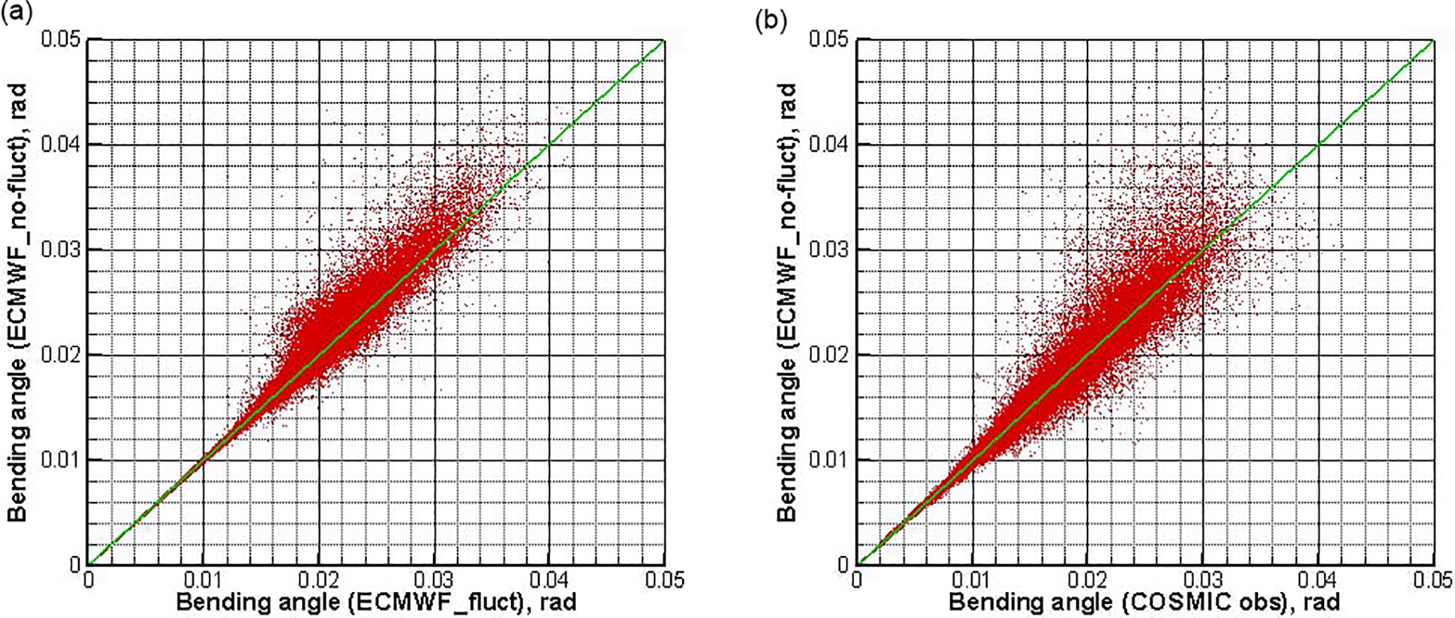
Figure 4 Scatter plot of fluctuation-affected bending angle profiles (x axis) from ECMWF-based simulations with refractivity fluctuations superposed (a) and from COSMIC observations (b) versus reference bending angle profiles (y axis) from ECMWF simulations without refractivity fluctuations superposed. COSMIC events and concurrent ECMWF analysis fields from the 15th and 16th day of every month of year 2008 were used for these example results.

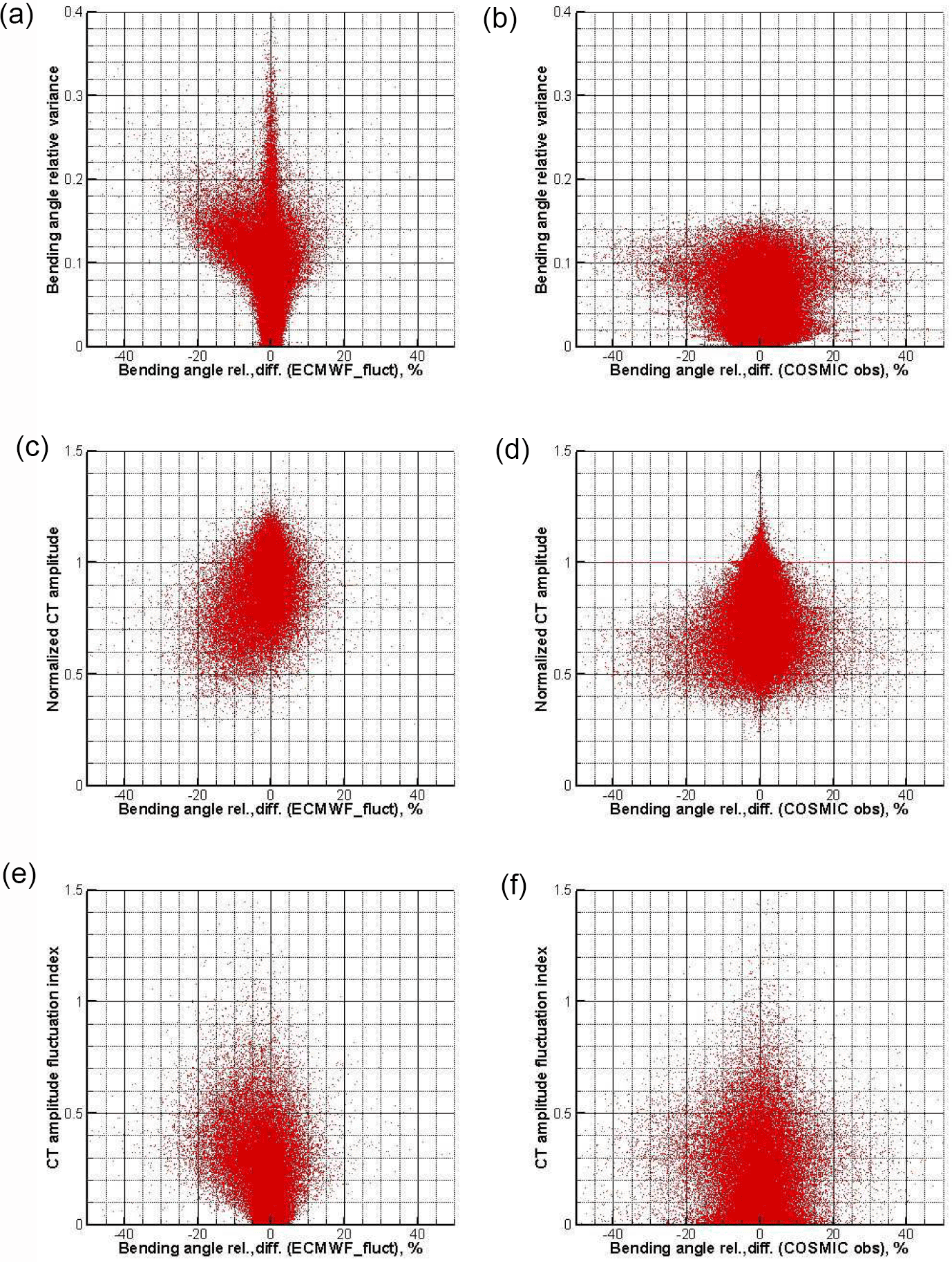
Figure 5 Scatter plot of the difference of fluctuation-effected and reference bending angle profiles (x axis) for ECMWF simulations with refractivity fluctuations superposed (a, c, e) and COSMIC observations (b, d, f) versus the predictor variables (y axis) bending angle relative variance (a, b), normalized CT amplitude (c, d), and CT amplitude fluctuation index (e, f). The reference bending angles are from ECMWF simulations without refractivity fluctuations superposed. The same ECMWF fields and COSMIC data as for Fig. 4 were used.

Because we need to derive the regression model for widely diverse BLB behavior, we start with very general regression relations. Consider two series of random variables, vector x_i and scalar series y_i, where the lower index i enumerates the realizations. We will define the components of x_i predictors, because we approximate the random variables y_i as a linear combination of predefined adaptive functions φ^j of x_i. The number of predictors, and of associated adaptive functions, is much smaller than the number of realizations (difference profiles of observed and reference bending angles in the lower troposphere). We write the overdetermined system of equations as

$$\begin{array}{}\text{(1)}& {\displaystyle }& {\displaystyle }{y}_i=\sum _j{\mathit{\alpha }}^j{\mathit{\phi }}^j\left({\mathit{x}}_i\right)\equiv \sum _j{\mathit{\alpha }}^j{K}_{ij},\text{(2)}& {\displaystyle }& {\displaystyle }{K}_{ij}={\mathit{\phi }}^j\left({\mathit{x}}_i\right),\end{array}$$

or in the vector form,

$$\begin{array}{}\text{(3)}& \mathit{y}=\widehat{\mathbf{K}}\mathit{\alpha }.\end{array}$$

This system has a pseudo-inverse solution, i.e., the vector α that minimizes the discrepancy

$$\begin{array}{}\text{(4)}& {\left(\mathit{y}-\widehat{\mathbf{K}}\mathit{\alpha }\right)}^T\left(\mathit{y}-\widehat{\mathbf{K}}\mathit{\alpha }\right)=min\end{array}$$

is obtained as the least-squares solution of this overdetermined problem in the form

$$\begin{array}{}\text{(5)}& \mathit{\alpha }={\left({\widehat{\mathbf{K}}}^T\widehat{\mathbf{K}}\right)}^{-\mathrm{1}}{\widehat{\mathbf{K}}}^T\mathit{y}.\end{array}$$

Now consider a numerical estimation of α that allows for an evaluation readily augmentable in terms of the number of realizations and adaptive functions. Preparing the quadratic form

$$\begin{array}{}\text{(6)}& {\displaystyle }& {\displaystyle }\widehat{\mathbf{B}}={\widehat{\mathbf{K}}}^T\widehat{\mathbf{K}},\text{(7)}& {\displaystyle }& {\displaystyle }{B}_{ij}=\sum _k{K}_{ki}{K}_{kj}=\sum _k{\mathit{\phi }}^i\left({\mathit{x}}_k\right){\mathit{\phi }}^j\left({\mathit{x}}_k\right),\end{array}$$

we have available matrix $\widehat{\mathbf{B}}$ as a square symmetric matrix that can be evaluated by the summation over any existing set of realizations of x_i. Similarly, using the transform

$$\begin{array}{}\text{(8)}& {\displaystyle }& {\displaystyle }\mathit{z}=\widehat{\mathbf{K}}\mathit{y},\text{(9)}& {\displaystyle }& {\displaystyle }{z}_i=\sum _j{K}_{ij}{y}_j=\sum _j{\mathit{\phi }}^i\left({\mathit{x}}_j\right)y_j,\end{array}$$

we have available vector z as a vector that can also be evaluated by the summation over any existing set of realizations of x_i and y_i. Finally, it is straightforward in this formulation to obtain the regression coefficients from

$$\begin{array}{}\text{(10)}& \mathit{\alpha }={\widehat{\mathbf{B}}}^{-\mathrm{1}}\mathit{z}.\end{array}$$

For convenience, matrix $\widehat{\mathbf{B}}$ and vector z can be redefined in terms of averaging over the ensemble of realizations. Denoting N as the number of realizations, this is performed by dividing both $\widehat{\mathbf{B}}$ and z by N,

$$\begin{array}{}\text{(11)}& {\displaystyle }& {\displaystyle }{B}_{ij}={\displaystyle \frac{\mathrm{1}}{N}}\sum _k{\mathit{\phi }}^i\left({\mathit{x}}_k\right){\mathit{\phi }}^j\left({\mathit{x}}_k\right)=〈{\mathit{\phi }}^i{\mathit{\phi }}^j〉,\text{(12)}& {\displaystyle }& {\displaystyle }{z}_i={\displaystyle \frac{\mathrm{1}}{N}}\sum _j{\mathit{\phi }}^i\left({\mathit{x}}_j\right)y_j=〈{\mathit{\phi }}^{i}y〉.\end{array}$$

Practically, normalization can also be an issue, depending on the number of adaptive functions. If their number is as high as about 200, such as in our study (Sect. 2.4), then even a small change in the normalization factor is raised to the 200th power when evaluating the matrix determinant. This may result in overflow or underflow in the matrix inversion. Therefore, the numerical algorithm requires accurate tuning of the normalization factor in order to ensure a stable and robust inversion of matrix $\widehat{\mathbf{B}}$.

After having solved for the regression coefficient vector α, it can be used within Eq. (3), which then serves as the BLB model applicable to any given RO event. It will provide the estimated bending angle BLB profile y for the RO event when its predictors are used to specify the model matrix $\widehat{\mathbf{K}}$.

2.3 Predictors for the model's adaptive functions

Here we consider the predictors that we may reasonably choose. Besides predictors depending on RO event altitude and latitude (discussed separately below), we adopt the following four predictors that are derived from observational RO data – all as function of impact parameter p within the lower troposphere (below an impact altitude of 4.5 km): (1) bending angle ϵ(p), (2) bending angle standard deviation δϵ(p), (3) normalized CT amplitude A_CT(p), and (4) CT amplitude fluctuation index β(p). Bending angle standard deviation is the bending angle standard error estimate based on radio-holographic analysis (Gorbunov et al., 2006). The CT amplitude (Gorbunov, 2002; Gorbunov and Lauritsen, 2004) is the normalized energy distribution over rays in the impact parameter space. We use the CT amplitude normalized in such a way that it should equal unity in vacuum. The CT amplitude fluctuation index β(p) is defined as

$$\begin{array}{}\text{(13)}& \mathit{\beta }\left(p\right)={\widehat{S}}_{\mathit{\beta }}\left({\left(A_{\mathrm{CT}}\left(p\right)-\widehat{S}{A}_{\mathrm{CT}}\left(p\right)\right)}^{\mathrm{2}}\right),\end{array}$$

where ${\widehat{S}}_{\mathit{\beta }}$ is a smoothing operator (low-pass filter) for which we use a 2 km smoothing width.

Figure 4 shows the scatter plot of fluctuation-affected bending angles versus reference bending angles for the fluctuation-model simulations (like for Fig. 1) and the COSMIC observations (like for Fig. 2). In both cases the asymmetry with respect to the diagonal is visible (fluctuation-affected bending angles are tentatively smaller than reference ones). This indicates that the bending angle itself can serve as one meaningful predictor of (negative) boundary layer biases.

Figure 5 shows scatter plots of the difference of fluctuation-affected and reference bending angle profiles versus bending angle standard deviation (top), normalized CT amplitude (middle), and CT amplitude fluctuation index (bottom) for simulations (left) and COSMIC observations (right).

Comparing the behavior of these predictors, their correlation with the bending angle difference is clearly more salient in the simulations but some smaller asymmetry can also be noticed for the COSMIC observation differences. We therefore kept all four predictors in this study and left possible further reduction of these predictors (and associated adaptive functions) to future fine-tuning of the BLB model regression. An important conclusion from these comparisons is that the fluctuation model alone does not explain the patterns observed in the real observations. However, the role of this model is to help in finding reasonable predictors. The further bias correction procedure is only based on the predictors that can be readily derived from observations, rather than on the fluctuation model.

In addition to these four predictors we utilize the RO event coordinates (impact altitude z and latitude λ), where $z=p-R_{\mathrm{LC}}-U_{\mathrm{geoid}}$, with R_LC being the local radius of curvature and U_geoid the geoid undulation applying to the event location. We use the impact altitude z directly and in the form of the following six trigonometric functions of z:

$$\begin{array}{}\text{(14)}& \sin \left(\mathrm{2}\mathit{\pi }n{\displaystyle \frac{z-z_{\min }}{z_{\max }-z_{\min }}}\right),\cos \left(\mathrm{2}\mathit{\pi }n{\displaystyle \frac{z-z_{\min }}{z_{\max }-z_{\min }}}\right),n=\mathrm{1}\mathrm{\dots }\mathrm{3},\end{array}$$

where z_min and z_max are the limits of impact altitude wherein the BLB profiles are evaluated (equal to 1.5 and 4.5 km). Latitude λ is used in the form of another six trigonometric functions of λ,

$$\begin{array}{}\text{(15)}& \sin \left(n\mathit{\lambda }\right),\cos \left(n\mathit{\lambda }\right),n=\mathrm{1}\mathrm{\dots }\mathrm{3}.\end{array}$$

Altogether we therefore use N_p=17 predictors, including impact altitude, the four observation-derived predictors, six functions of impact altitude, and six functions of latitude. This number of predictors exceeds that in radiation correction schemes, where six to eight predictors are typically used (e.g., Zhu et al., 2014).

2.4 Construction of the model's adaptive functions

General adaptive functions as we use here are constructed in the form of different degrees of the predictors and their cross products from degree zero, which produces unity, up to some maximum degree D_p,

$$\begin{array}{}\text{(16)}& {\displaystyle }& {\displaystyle }\left\{{\mathit{\phi }}^j\left(\mathbf{x}\right)\right\}=\left\{\mathrm{1},{\left(x^i\right)}^{\mathit{\gamma }},{\left(x^{i_{\mathrm{1}}}\right)}^{{\mathit{\gamma }}_{\mathrm{1}}}{\left(x^{i_{\mathrm{2}}}\right)}^{{\mathit{\gamma }}_{\mathrm{2}}}\right\},\text{(17)}& {\displaystyle }& {\displaystyle }\mathrm{1}\le i\le N_p,\mathrm{1}\le \mathit{\gamma }\le D_p,\text{(18)}& {\displaystyle }& {\displaystyle }\mathrm{1}\le i_{\mathrm{1}}<i_{\mathrm{2}}\le N_p,\mathrm{1}\le {\mathit{\gamma }}_{\mathrm{1}}+{\mathit{\gamma }}_{\mathrm{2}}\le D_p,{\mathit{\gamma }}_{\mathrm{1},\mathrm{2}}>\mathrm{0}.\end{array}$$

We use a maximum degree of D_p=3 and apply some additional constraints in order to reduce the number of adaptive functions. For the six trigonometric functions of impact altitude (Eq. 14), taking their degrees beyond degree 1 and their cross products is not allowed as these will not be linearly independent from other trigonometric functions of the impact altitude. The same applies to the six trigonometric functions of latitude (Eq. 15) for which we therefore also disregard degrees beyond degree 1 and cross products.

For our choice of D_p=3 we thus obtain N_f=214 adaptive functions. To understand this number, consider different degrees of predictors. There is one zero-degree function (unity). There are 17 functions of degree 1 (the 17 predictors). There are $\mathrm{6}\times (\mathrm{6}+\mathrm{5})+\mathrm{6}\times \mathrm{5}+(\mathrm{5}\times \mathrm{4})/\mathrm{2}+\mathrm{5}=\mathrm{111}$ functions of degree 2. There are $\mathrm{2}\times \mathrm{6}\times \mathrm{5}+\mathrm{5}+\mathrm{5}\times \mathrm{4}=\mathrm{85}$ functions of degree 3. Therefore, we arrive in total at $\mathrm{1}+\mathrm{17}+\mathrm{111}+\mathrm{85}=\mathrm{214}$ adaptive functions, which provide the needed flexibility for the highly variable BLB profile behavior while still allowing for a robust estimation of the regression coefficients. If future fine-tuning of the regression model were to reduce the number of predictors, the number of adaptive functions would reduce accordingly.

2.5 Simple residual systematic uncertainty model

As described in Sect. 2.2, after obtaining the regression coefficient vector (Eq. 10), we can use it within the regression model (Eq. 3), which then serves as the BLB model applicable to any given RO event. It provides the bending angle BLB model profile for the RO event, δα_BLB(z), based on its predictors depending on location (impact altitude, latitude) and bending angle and CT amplitude characteristics (Sect. 2.3).

Given this basis, we define a simple initial systematic uncertainty model for the BLB-corrected bending angle profiles of the lower troposphere, $u_{\mathit{\delta }\mathit{\alpha },\mathrm{BLB}}^{\mathrm{s}}\left(z\right)$, which consists of two components: (1) an estimated lower-bound ECMWF-reference field-induced systematic uncertainty, $u_{\mathrm{refEC}}^{\mathrm{s}}$, that accounts for the uncertainty from using the ECMWF analysis fields as the regression reference, which have their own (small) systematic deviations from the truth, and (2) an estimated residual bias uncertainty after BLB correction by subtracting the BLB model profile, $u_{\mathrm{resBLB}}^{\mathrm{s}}$, since the empirical–statistical BLB regression model can never fully fit the individual bias situation of an RO event.

From experience with estimated biases of ECMWF analysis fields in other studies (e.g., Li et al., 2013, 2015; Scherllin-Pirscher et al., 2017; Li et al., 2017), we formulate the model for the ECMWF-reference field-induced systematic uncertainty profile $u_{\mathrm{refEC}}^{\mathrm{s}}\left(z\right)$ as a fractional model ($f_{\mathrm{refEC}}^{\mathrm{us}}\left(z\right)$) with a linear increase downward over the lower troposphere towards the surface,

$$\begin{array}{}\text{(19)}& \mathrm{100}\cdot {\displaystyle \frac{u_{\mathrm{refEC}}^{\mathrm{s}}\left(z\right)}{{\mathit{\alpha }}_{\mathrm{refEC}}\left(z\right)}}=f_{\mathrm{refEC}}^{\mathrm{us}}\left(z\right)=f_{\mathrm{refEC},\mathrm{zmin}}^{\mathrm{us}}\cdot {\displaystyle \frac{(z_{\max }-z)}{(z_{\max }-z_{\min })}},\end{array}$$

where α_refEC(z) is the ECMWF reference bending angle profile, z_min and z_max are the limits of impact altitude (set to 1.5 and 5.0 km), and $f_{\mathrm{refEC},\mathrm{zmin}}^{\mathrm{us}}$ is the fractional uncertainty at z_min empirically set to 0.25 %. For perspective, the bending angle uncertainties obtained this way correspond in terms of temperature to uncertainties from about 0.2 K near 4 km impact altitude to 0.6 K near the surface (for details on uncertainty relations among RO-derived variables see Scherllin-Pirscher et al., 2011b, 2017, and references therein).

The estimated residual bias uncertainty profile after BLB correction is formulated from experience with other bias corrections, such as sampling bias correction (e.g., Scherllin-Pirscher et al., 2011a, 2017), and based on BLB correction performance results with test ensembles during this study in a straightforward fractional form,

$$\begin{array}{}\text{(20)}& u_{\mathrm{resBLB}}^{\mathrm{s}}\left(z\right)=r_{\mathrm{resBLB}}\cdot \mathit{\delta }{\mathit{\alpha }}_{\mathrm{BLB}}\left(z\right),\end{array}$$

where r_resBLB is the systematic uncertainty reduction factor empirically set to 0.2, i.e., expressing that due to the BLB correction the bias in the bending angle profile is reduced by a factor of 5.

For the estimated residual systematic uncertainty finally attributed to the BLB-corrected lower-tropospheric bending angle at any impact altitude, we then simply adopt the larger one of the two uncertainties,

$$\begin{array}{}\text{(21)}& u_{\mathit{\delta }\mathit{\alpha },\mathrm{BLB}}^{\mathrm{s}}\left(z\right)={\widehat{S}}_{\mathrm{us}}\left(\mathrm{Max}\left(u_{\mathrm{resBLB}}^{\mathrm{s}}\left(z\right),u_{\mathrm{refEC}}^{\mathrm{s}}\left(z\right)\right)\right),\end{array}$$

implementing the lower-bound uncertainty role of $u_{\mathrm{refEC}}^{\mathrm{s}}$ in cases where the estimated residual bias uncertainty $u_{\mathrm{resBLB}}^{\mathrm{s}}$ of individual RO events according to Eq. (20) is occasionally very small. ${\widehat{S}}_{\mathrm{us}}$ is a smoothing operator (low-pass filter) with a 0.4 km filter width that we use to ensure adequate smoothness of the resulting $u_{\mathit{\delta }\mathit{\alpha },\mathrm{BLB}}^{\mathrm{s}}\left(z\right)$ profile also over those altitude levels where the two uncertainty components cross in their magnitude.

3 Wave-optical propagation of systematic and random uncertainties

The propagation of systematic and random uncertainties through the wave-optical retrieval chain was investigated by Gorbunov and Kirchengast (2015), where a simple approximation was derived and verified based on numerical simulations (as summarized in Sect. 1). The approximation considers the excess phase as function of time, Ψ(t), and its systematic (small-scale) and random (large-scale) uncertainties, Σ₁(t) and Σ₂(t), respectively. The uncertainty in the impact parameter space (Gorbunov and Lauritsen, 2004) is then evaluated as ${\stackrel{\mathrm{̃}}{\mathrm{\Sigma }}}_{\mathrm{1},\mathrm{2}}\left(p\right)={\mathrm{\Sigma }}_{\mathrm{1},\mathrm{2}}\left(t\left(p\right)\right)$, where t(p) is the time of observation of the ray with impact parameter p.

Practically the application of this approximation was shown by Gorbunov and Kirchengast (2015) to work well for propagating random uncertainties (covariance matrices), while in sensitivity tests and evaluations for this study we found that it does not work sufficiently well for propagating systematic uncertainties, due to the large-scale nature of such (increment) profiles not transforming smoothly under FIO operations (Gorbunov and Lauritsen, 2004). Similarly, given the BLB and residual systematic uncertainty model being formulated in terms of bending angle, the inverse transformation of these into the equivalent excess phase bias and uncertainty proves to be not straightforward either.

The reason and underlying problem is that the perturbation of the excess phase due to the superimposing of the systematic uncertainty of the bending angle is not smooth. The variation in the bending angle profile in each realization results in the different phase perturbation corresponding to a different ray manifold with a different caustic structure. Therefore, the excess phase perturbation has a complicated nonlinear relation with the phase (eikonal) uncertainty in impact parameter space, and this perturbation corresponds to a complicated coherent signal being a superposition of multiple signals corresponding to different rays.

To overcome this difficulty, we do apply the linearized approximation only for the propagation of random uncertainty, i.e., the covariance propagation according to Gorbunov and Kirchengast (2015) – Eqs. (29) and (30) therein. This is applied within the rOPS wave-optical retrieval, for both GNSS frequencies, right after the bending angle profiles themselves have been retrieved by the (forward) FIO in the CT2 implementation (Gorbunov and Lauritsen, 2004; Gorbunov, 2011). The BLB and estimated systematic uncertainty propagation is then computed, in a consistent way for bending angles and excess phases, with a perturbation approach in a three-step sequence as follows.

First, the BLB profile and its estimated systematic uncertainty profile after BLB subtraction are computed according to Sect. 2.5 for the lower-tropospheric bending angle profile at the L1 frequency, for the location and characteristics (i.e., the applicable predictors) of the given RO event. It is not computed for the second (L2) frequency, since the L2 profiles are generally more noisy (making BLB estimation difficult) and not further used at impact altitudes below 5 km. Below this level, where the neutral atmospheric excess phase always exceeds several hundreds of meters, the dual-frequency ionospheric correction instead always uses L1–L2 difference bending angles extrapolated from above (Schwarz et al., 2017b), avoiding noise amplification and mitigating potentially adverse effects on top-of-boundary-layer estimates recently pointed out by Sokolovskiy et al. (2016).

Second, the BLB-corrected L1 bending angle profile and this profile perturbed by the estimated systematic uncertainty profile are each projected back to excess phase by applying the inverse FIO approach recently introduced by Gorbunov (2016). This provides the BLB-corrected L1 excess phase profile and, from the difference of the two back-projected profiles, the estimated systematic excess phase uncertainty profile pertaining to it. The latter BLB-related systematic uncertainty is then added (in a root-mean-square sense) to the basic systematic excess phase uncertainty available from the raw processing towards excess phase (Innerkofler et al., 2016), yielding the total estimated systematic excess phase uncertainty profile.

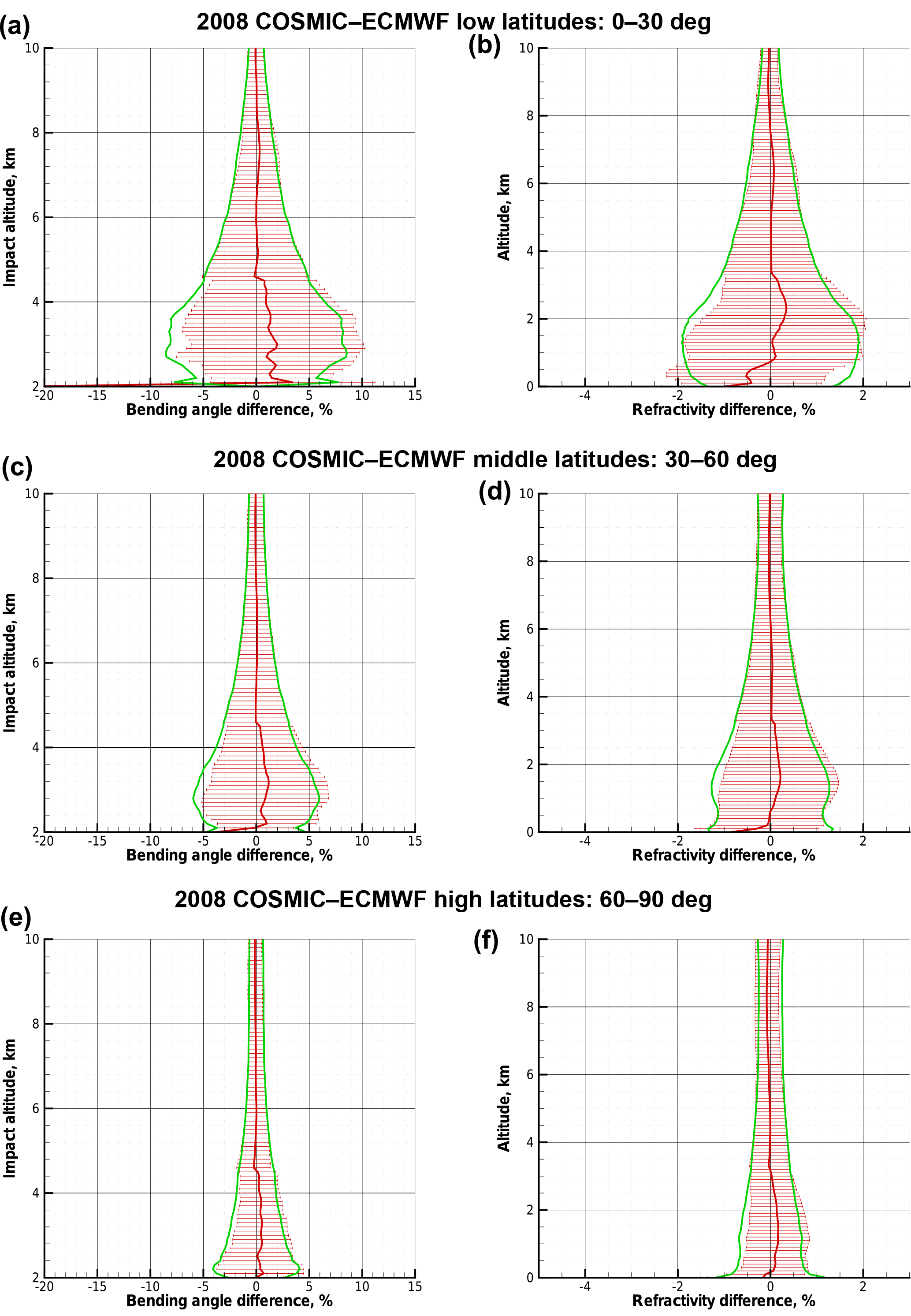
Figure 6 Deviation statistics based on original BLB-corrected bending angles: difference statistics of COSMIC profiles relative to ECMWF reference profiles, with the same layout of panels as for Fig. 2, for bending angle as function of impact altitude (a, c, e) and refractivity as function of altitude (b, d, f). Results for low latitudes (a, b), midlatitudes (c, d), and high latitudes (e, f) are shown, based on COSMIC data from the 17th day of every month of year 2008 and concurrent ECMWF analysis fields.

Third, the BLB-corrected L1 excess phase profile and this profile perturbed by the total estimated systematic uncertainty profile are processed again through the standard (forward) FIO CT2-wave-optics retrieval in order to obtain a BLB-corrected retrieved bending angle profile, for a consistency check with the original BLB-corrected bending angle profile, as well as the total estimated systematic bending angle uncertainty profile, from the difference of the two CT2-retrieved bending angle profiles. The systematic bending angle uncertainty profile at the second (F2) frequency is finally obtained from also processing the L2 excess phase profile perturbed by its associated systematic uncertainty through the wave-optics retrieval and estimating it from the difference of the resulting perturbed bending angle profile to the one originally retrieved from the unperturbed L2 excess phase.

Despite of the complexities from the nonlinearities involved, we obtain in this way a consistent set of excess phase and bending angle profiles together with their estimated systematic and random uncertainties, which are BLB-corrected at the L1 frequency in the lower troposphere. The extra computational expense for the uncertainty propagation due to the nonlinearity is reasonably limited to one additional forward and inverse FIO operation at L1 frequency, which is required for the perturbation approach to systematic uncertainty propagation. This is similar to the uncertainty propagation work of Schwarz et al. (2017a, b), where the perturbation approach is also needed in a small number of steps (during geometric-optics bending angle retrieval and dry-air temperature retrieval) for the systematic uncertainty propagation.

4 Results

Here we evaluate the consistency of the BLB-corrected bending angles and their associated retrieved refractivities by (i)  using the original BLB-corrected bending angles and (ii) back-projecting the original BLB-corrected retrieved bending angles to obtain BLB-corrected excess phases and then retrieving the bending angles again. This provides a basic validation of our procedure as described in Sect. 3; to limit the extent of this paper, the detailed inspection and validation of the uncertainty propagation itself is left for a follow-on study.

We investigated the BLB correction of an independent ensemble of COSMIC-retrieved bending angles employing our BLB model, as in Sect. 2.1 using ECMWF analysis fields as reference. Figure 6 shows the COSMIC–ECMWF difference statistics of bending angles (left) and refractivities (right) after bending angle BLB correction. These statistics were evaluated for a set of 12 days of COSMIC data from year 2008, including the 17th day of every month, amounting in total to about 26 000 RO events. This implies that these COSMIC and ECMWF ensembles of profiles are independent from the ones used in the derivation of the BLB model regression coefficients (the 15th and 16th day of every month; see Sect. 2.1).

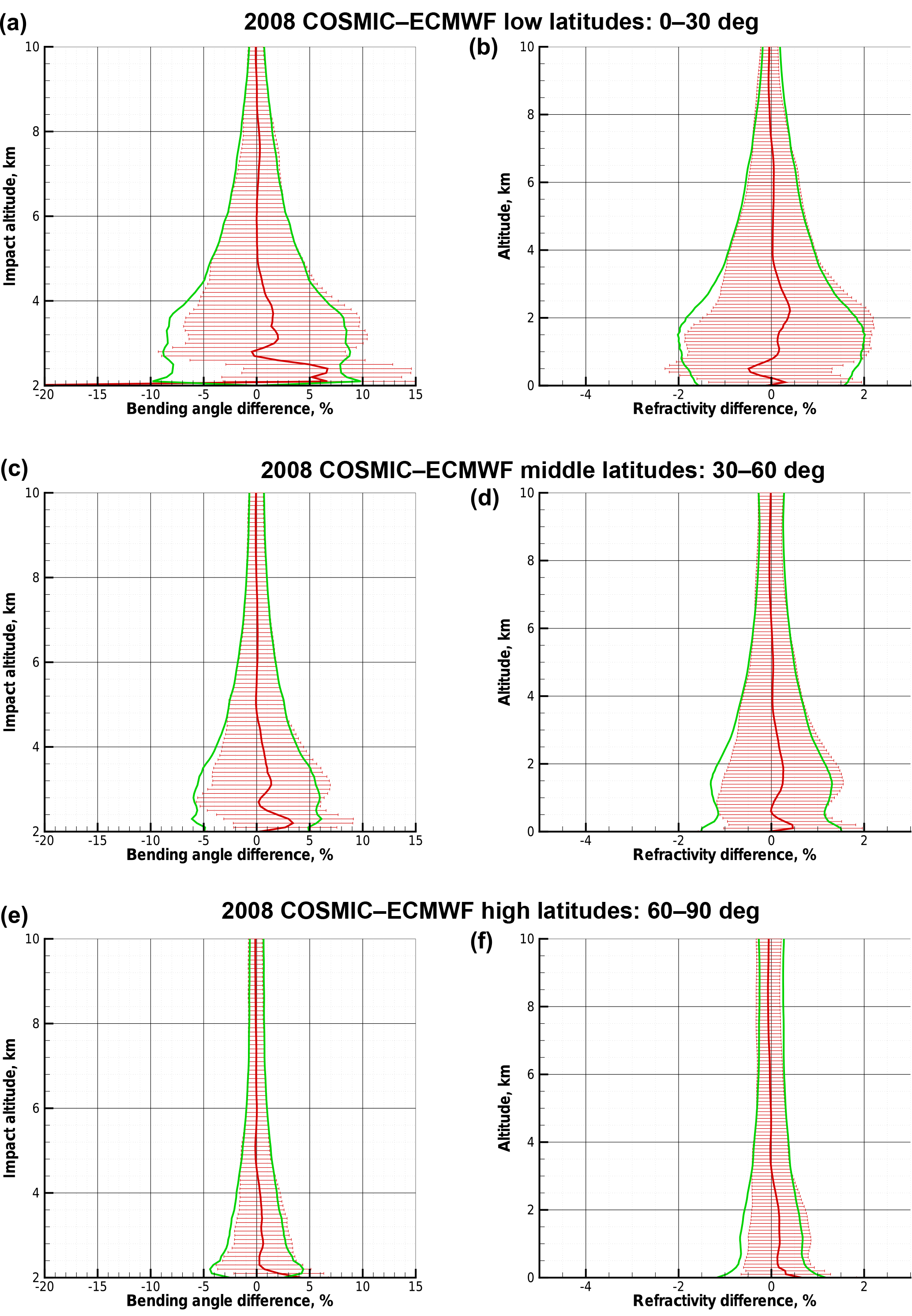
Figure 7 Deviation statistics based on BLB-corrected retrieved bending angles (after back projection of original BLB-corrected bending angles to excess phases and in turn retrieving the bending angles again): COSMIC–ECMWF difference statistics with the same layout and using the same COSMIC and ECMWF data as for Fig. 6.

Cross-checking these results with results from COSMIC and ECMWF ensembles using the 16th day of every month (not separately shown), we find them practically indistinguishable in terms of their difference statistics. This indicates the statistical homogeneity of the data sets and the robustness of the BLB model. Furthermore, from comparing Fig. 6 with Fig. 2, it is clear that the BLB correction achieves a substantial decrease in the boundary layer biases by about a factor of 5, which is consistent with the systematic uncertainty reduction factor r_resBLB=0.2 (Eq. 20). Immediately above the boundary layer, above about 2 km altitude, the BLB-corrected profiles possibly contain slightly increased uncertainty, at a small magnitude, which is accounted for by the reference field-induced lower-bound uncertainty $u_{\mathrm{refEC}}^{\mathrm{s}}$ (Eq. 19) included in the systematic uncertainty model up to 5 km impact altitude. This may be improved in the future by a further-refined BLB model design.

Figure 7 shows the COSMIC–ECMWF difference statistics of bending angles (left) and refractivities (right) based on the BLB-corrected bending angles obtained by back-projecting the original BLB-corrected bending angles by the inverse FIO to obtain BLB-corrected excess phases and then retrieving the bending angles again. Except for about the lower half of the kilometer above surface where there is possibly some degradation, the results are found very close to those shown in Fig. 6 for the original BLB-corrected bending angles. This indicates the basic validity and robustness of our approach to transfer the BLB-corrected bending angles to BLB-corrected excess phases. Future more detailed inspection of the full uncertainty propagation approach according to Sect. 3 will consolidate this encouraging initial validation.

Figure 8 presents a latitude–longitude map of the COSMIC–ECMWF difference at a height of 0.6 km in terms of systematic relative refractivity deviation, similar to Fig. 3, but after the BLB correction applied to the underlying bending angles. This plot indicates that, although the overall average bias is minimized, there are some regional maxima and minima. Some of them correspond to the areas with a sharp marine boundary layer (Xie et al., 2006, 2010; Gorbunov, 2014), where the negative bias is reduced but still remains. Other regions with larger deviations are located above northern Africa and Australia, where there is a positive overcorrection. The latter regions correspond to a similar terrain type, i.e., dry desert areas. This indicates the need for refined predictors, taking into account such regional effects, in order to further mitigate in a next step these more specific biases.

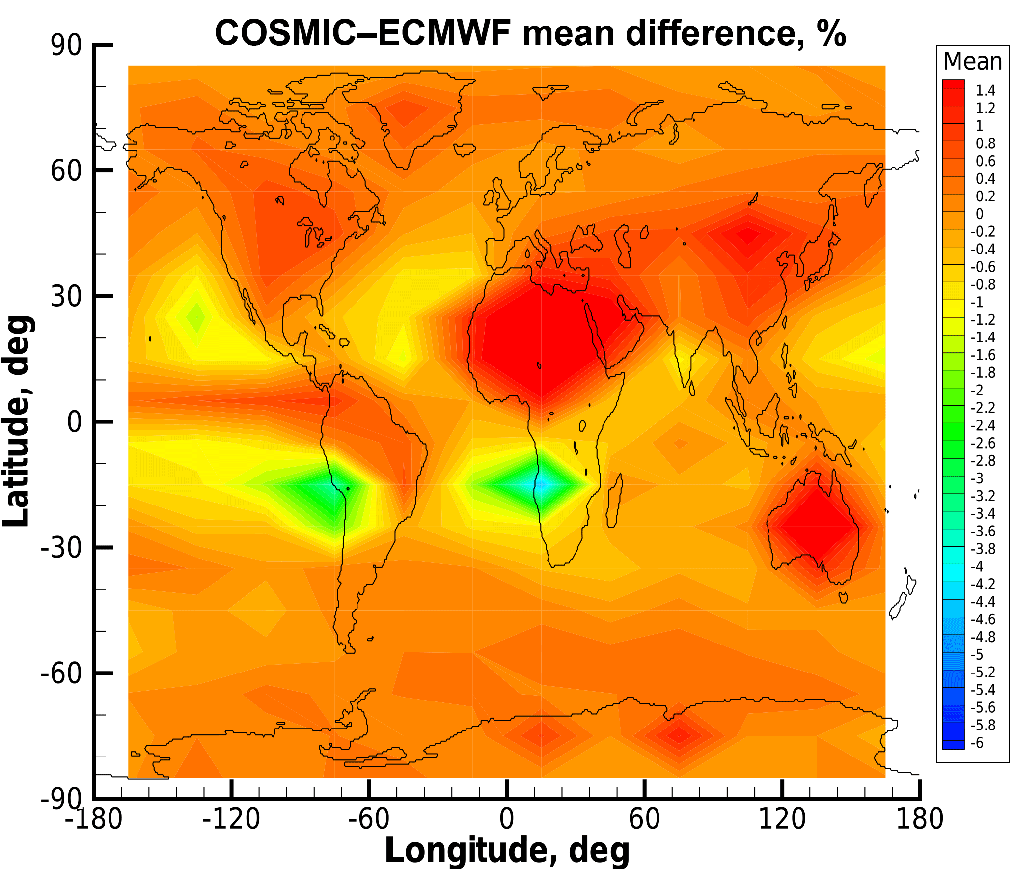
Figure 8 Deviation statistics based on original BLB-corrected bending angles: latitude–longitude map (10^∘ lat × 30^∘ long grid resolution) of difference statistics of COSMIC observations relative to ECMWF profiles without fluctuations for refractivity at an altitude of 0.6 km. Results are shown for COSMIC events and concurrent ECMWF analysis fields from the 1st, 11th, and 21st day of every month of year 2008.

5 Conclusions

In this study we developed a regression-based approach for modeling and propagating the atmospheric boundary layer biases and associated (residual) systematic uncertainties within the wave-optical retrieval chain of the reference occultation processing system, which is a new RO processing system with integrated uncertainty propagation that focuses on calibration–validation and climate applications.

Currently, there is no quantitative physical model describing BLB in RO data, although there was a series of studies discussing different mechanisms resulting in BLB. The starting point encouraging and informing our BLB model design was the fluctuation-based explanatory modeling of the well-known negative refractivity bias problem in the boundary layer. We showed that it is possible to achieve a reasonable agreement with observed bending angle and refractivity biases by modeling fluctuation statistics consistent with reasonable tropospheric profiles of the refractivity structure constant $C_N^{\mathrm{2}}\left(z\right)$.

Based on this understanding we can robustly assume that reliable modeling of the bending angle BLB, and subsequent use of the model for BLB correction, will also effectively mitigate biases in the retrieved refractivity profiles and further-derived atmospheric profiles. However, given the highly variable refractivity fluctuations affecting individual RO events in reality, which implies a complex dependence of the bending angle BLB on the location and the data characteristics of individual RO profiles, we found it necessary to implement a BLB model with a very flexible functional behavior in order to reliably serve its purpose.

We therefore have chosen a versatile empirical regression-modeling approach and found suitable predictors of the BLB in the lower-tropospheric bending angle, including the bending angle and its standard deviation, CT amplitude and its fluctuation index, impact altitude and its trigonometric functions, and trigonometric functions of latitude. Degrees and cross products of these predictors were used to form a set of flexible adaptive functions that served as the basis for the BLB model, which was then obtained by regression to a large ensemble of COSMIC and ECMWF profile differences. Also, a simple (residual) systematic uncertainty model was formulated, applying to the bending angles after BLB correction. For any given RO event, the BLB model profile can be computed based on the predictors that purely depend on the event location and the characteristics of the bending angle and CT amplitude profiles.

Together with the linearized wave-optics (random) uncertainty propagation approach described by Gorbunov and Kirchengast (2015), we used the new approach to formulate the algorithmic sequence for wave-optical retrieval of bending angles from excess phases including consistent BLB correction and the associated random and systematic uncertainty propagation. Evaluating the consistency of the BLB-corrected bending angles and their associated retrieved refractivities we achieved a successful basic validation of the new procedure: we found that the BLB correction delivers a substantial decrease in the boundary layer biases by about a factor of 5, which is consistent with our initial model of residual systematic uncertainty.

Our bias model uses ECMWF fields as a reference; therefore, it involves the biases that are intrinsic to these ECMWF fields. However, the same approach can be applied together with an independent estimate of the ECMWF biases. In this study, we assumed that ECMWF biases form a small fraction of the observed systematic COSMIC–ECMWF differences.

These results are encouraging for follow-on work in the near future that can provide a refined BLB model design and a detailed inspection and validation of the complete wave-optical retrieval and uncertainty propagation as introduced in this study. In this way, the rOPS geometric-optical bending angle retrievals (Schwarz et al., 2017b), generally available reliably from the middle troposphere upwards, can be complemented and merged, from the upper troposphere downwards, with these wave-optical bending angle retrievals. Jointly this provides high quality of the RO data and their integrated uncertainty estimates from the stratosphere down close to the surface.