Measurement of atmospheric CO₂ column concentrations to cloud tops with a pulsed multi-wavelength airborne lidar

We have measured the column-averaged atmospheric CO₂ mixing ratio to a variety of cloud tops by using an airborne pulsed multi-wavelength integrated-path differential absorption (IPDA) lidar. Airborne measurements were made at altitudes up to 13 km during the 2011, 2013 and 2014 NASA Active Sensing of CO₂ Emissions over Nights, Days, and Seasons (ASCENDS) science campaigns flown in the United States West and Midwest and were compared to those from an in situ sensor. Analysis of the lidar backscatter profiles shows the average cloud top reflectance was ∼ 5 % for the CO₂ measurement at 1572.335 nm except to cirrus clouds, which had lower reflectance. The energies for 1 µs wide laser pulses reflected from cloud tops were sufficient to allow clear identification of CO₂ absorption line shape and then to allow retrievals of atmospheric column CO₂ from the aircraft to cloud tops more than 90 % of the time. Retrievals from the CO₂ measurements to cloud tops had minimal bias but larger standard deviations when compared to those made to the ground, depending on cloud top roughness and reflectance. The measurements show this new capability helps resolve CO₂ horizontal and vertical gradients in the atmosphere. When used with nearby full-column measurements to ground, the CO₂ measurements to cloud tops can be used to estimate the partial-column CO₂ concentration below clouds, which should lead to better estimates of surface carbon sources and sinks. This additional capability of the range-resolved CO₂ IPDA lidar technique provides a new benefit for studying the carbon cycle in future airborne and space-based CO₂ missions.

1 Introduction

Precise and accurate atmospheric CO₂ measurements with global coverage and full seasonal sampling are crucial to advance carbon cycle sciences (Schimel et al., 2016). Passive remote sensing of column-averaged atmospheric CO₂ mixing ratio (XCO₂) from space using Earth's surface-reflected sunlight, e.g., the US Orbiting Carbon Observatory (OCO-2; Crisp et al., 2004) and the Japanese Greenhouse gases Observation SATellite (GOSAT; Kuze et al., 2009), is limited to cloud-free pixels, where the photon path length can be well characterized. However those missions are unable to provide quality retrievals in the presence of clouds and aerosols due to significant modification of the photon path length by scattering (e.g., Mao and Kawa, 2004; Houweling et al., 2005; Aben et al., 2007; Butz et al., 2009; Uchino et al., 2012; Yoshida et al., 2013; Guerlet et al., 2013). Passive remote-sensing data from space thus are limited in spatial coverage and seasonal sampling, which may cause large uncertainty in regional and hemispheric carbon flux estimates (Chevallier et al., 2014; Reuter et al., 2014; Feng et al., 2009, 2016, 2017).

Active (lidar-based) remote sensing of CO₂ from space will carry its own optical source and so will allow day and night measurements and global sampling throughout the year. Range-resolved laser measurements allow accurate determination of the photon path length and thus enable accurate retrievals of XCO₂ to the scattering surface, even in the presence of thin clouds and aerosols. Because of these benefits the US National Research Council recommended the NASA Active Sensing of CO₂ Emissions over Nights, Days, and Seasons (ASCENDS) mission in the 2007 report Earth Science and Applications from Space: National Imperatives for the Next Decade and Beyond (National Research Council, 2007; http://www.nap.edu/catalog/11820.html).

The NASA Goddard Space Flight Center (GSFC) has developed a pulsed multi-wavelength integrated-path differential absorption (IPDA) lidar called the CO₂ Sounder to measure atmospheric CO₂ from space as a candidate for NASA's ASCENDS mission (Abshire et al., 2010, 2013, 2014, 2017). It uses a time-resolved receiver to record the altitude-resolved laser backscatter profiles at all measurement wavelengths, which enables accurate ranging to cloud tops and other targets. This allows retrieval of partial-column XCO₂ to cloud tops in addition to those for the full column to the ground. The difference in absorption line shapes between the full column and the partial column to cloud tops can be used to estimate partial-column XCO₂ between the ground and cloud tops for lower-layer atmospheric CO₂ (Ramanathan et al., 2015).

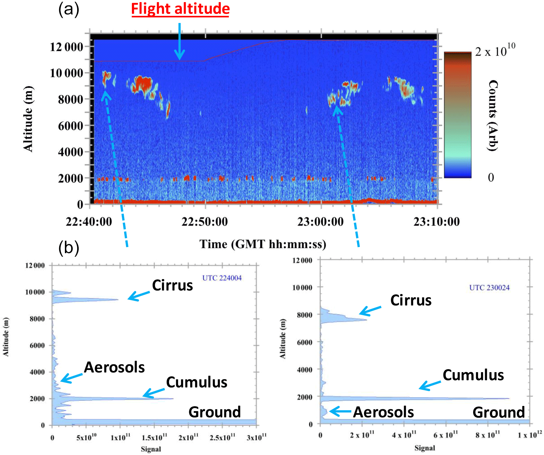
Figure 1 A 30 min long vertical cross section (a) and two individual 1 s vertical profiles (b) of atmospheric backscattering at offline wavelengths of CO₂ line measured by NASA GSFC CO₂ Sounder near the West Branch, Iowa, tall-tower site on 11 August 2011. The backscatter signals were corrected by square of range and averaged by 1 µs vertical running mean (∼ 150 m) and 1 s horizontal running mean (200 m of ground track). Returns from ground, cumulus and cirrus clouds, and aerosols are illustrated and labeled.

The GSFC CO₂ Sounder has been flown on NASA DC-8 aircraft since 2010 over a variety of sites in the US, along with other ASCENDS airborne lidar candidates together with accurate in situ CO₂ sensors. This paper describes the retrievals and analyses of partial-column XCO₂ measurements made to cloud tops for a variety of cloud types during the 2011, 2013 and 2014 ASCENDS airborne campaigns.

2 Measurement approach

The airborne CO₂ Sounder lidar uses a tunable narrow line width laser to measure CO₂ absorption at 30 wavelengths across the vibration–rotation line of CO₂ centered at 1572.335 nm. The line has a Lorentz half-width α_L≈ 0.07 cm⁻¹ (∼ 17 pm or 2.1 GHz) at standard atmospheric pressure and temperature. The laser is pulsed in a width of 1 µs at a rate of 10 kHz (or a step of 100 µs), and the laser scans across the CO₂ line at 30 wavelengths at a 300 Hz rate. The wavelength of each pulse was increased by 450 MHz or 0.015 cm⁻¹ uniformly for 2011 and 2013 campaigns. The sampling spacing was changed for the 2014 campaign to be 250 MHz near line center and 2 GHz or 0.067 cm⁻¹ on line wings to allow for more online samples. The laser line width is approximately 15 MHz or 0.0005 cm⁻¹. The laser's spectral resolution is considerably higher than that of GOSAT (∼ 0.2 cm⁻¹; Kuze et al., 2009), OCO-2 (∼ 0.3 cm⁻¹; Crisp et al., 2004) and the ground-based Fourier transform spectrometers of the Total Carbon Column Observing Network (TCCON; ∼ 0.02 cm⁻¹; Wunch et al., 2011). The narrow line width allows the measured CO₂ line shape to be fully resolved, including line width and line center position (Ramanathan et al., 2013). The parameters of the GSFC CO₂ Sounder have been summarized in tables of previous publications (Abshire et al., 2010, 2013, 2014).

The CO₂ Sounder is mounted in a fixed nadir-pointed orientation, which results in vertically directed measurements from the aircraft during normal horizontal flights. However, when the aircraft tilts, the laser points off-nadir, and the laser measurement direction is accounted for in the data processing. The laser photons backscattered from the atmosphere and ground are collected by a 20 cm receiver telescope, pass through a narrow (∼ 1 nm) band-pass filter, and then are focused onto the lidar detector. The bandwidth of receiver is 10 MHz, and it has a response time of 30 ns. The range backscatter profiles are accumulated and recorded after being averaged for all laser wavelengths at a 10 Hz rate to improve signal-to-noise ratio (SNR). The lidar measures range to better than 0.25 m to flat surfaces over a horizontal path from the laboratory (Amediek et al., 2013).

In the following sections, we briefly describe and illustrate GSFC CO₂ Sounder measurements, including backscattering, range, surface roughness and surface reflectance that enable retrievals of the partial-column XCO₂ to cloud tops.

2.1 Backscatter measurements

As an example, Fig. 1 shows a 30 min duration of backscatter profiles measured over Iowa during the 2011 ASCENDS airborne science campaign. The figure shows height-resolved lidar returns from the ground and from the top of fair-weather cumulus clouds at the top of the planetary boundary layer (PBL) near 2 km as well as from the body of high-altitude cirrus clouds. Some distributed aerosols were present, particularly within the boundary layer, but the signal was weak. The backscatter profiles at two discrete times are also shown.

2.2 Range measurements and surface roughness

The laser pulse energies from each significant scattering surface can be processed at each of the 30 transmitted wavelengths to display CO₂ line absorption features in terms of optical depth (OD). An example is shown in Fig. 2. These samples of the absorption line shape may be used to retrieve XCO₂ from aircraft altitude to each significant scattering surface by fitting measured ODs to pre-calculated ODs for the same atmospheric state. The ranging capability of pulsed lidar allows accurate determination of photon path length for XCO₂ retrievals. This is a major advantage of this lidar approach over passive approaches for remote sensing of greenhouse gases when the reflecting surface elevation is uncertain (e.g., cloud tops tall trees) and when the atmosphere has significant scattering (Mao and Kawa, 2004; Aben et al., 2007).

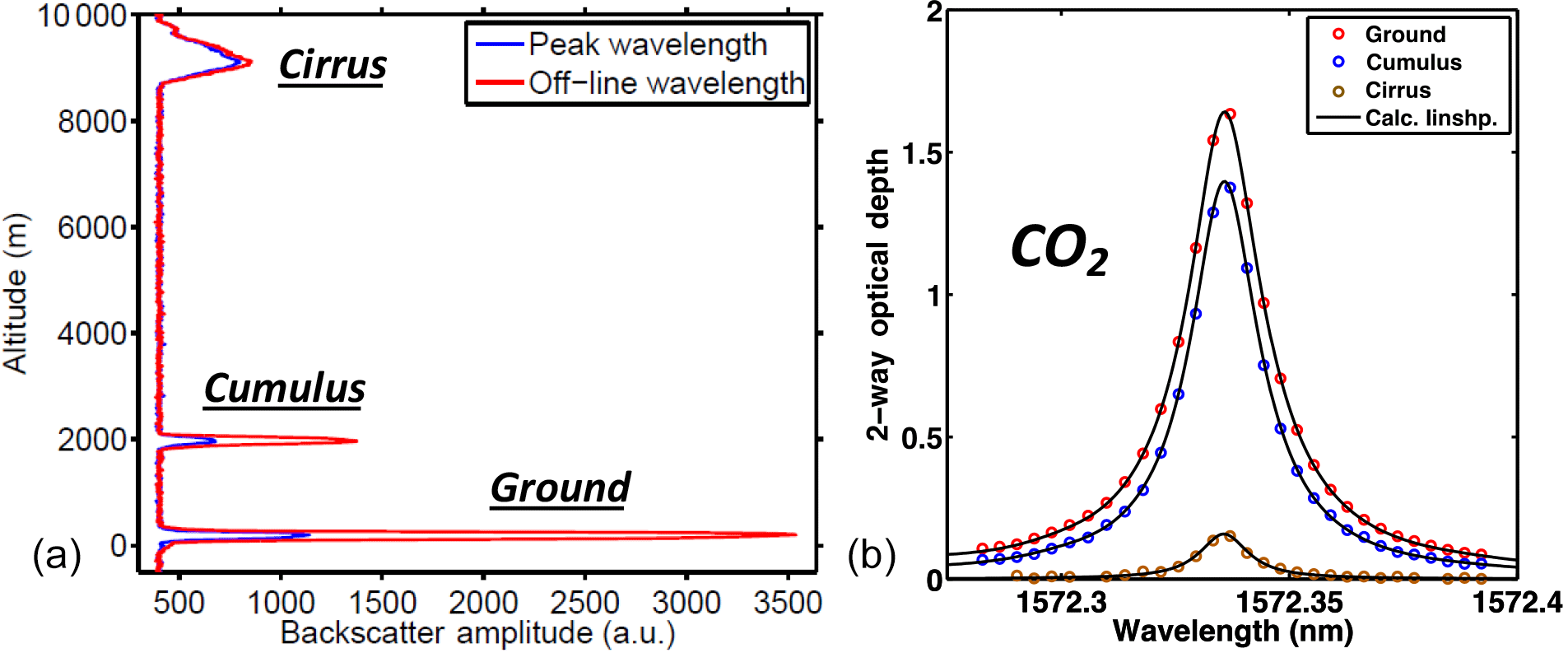
Figure 2 Backscatter profile (a) and CO₂ absorption line shapes (b) in terms of optical depth for laser returns from ground, cumulus clouds and cirrus clouds from a flight altitude of 12 km near the West Branch, Iowa, tall-tower site on 10 August 2011. In the left panel, the offline backscatter profile is plotted in red, and the backscatter profile at line center with peak absorption is plotted in blue. Both optical depth and differential optical depth between offline and line center wavelength increase with photon path length or range between aircraft and the scattering surface. Data are averaged over 10 s of ground track for both plots. In the right panel the dots are the lidar measurements and the solid lines are the best-fit line shapes from the XCO₂ retrievals.

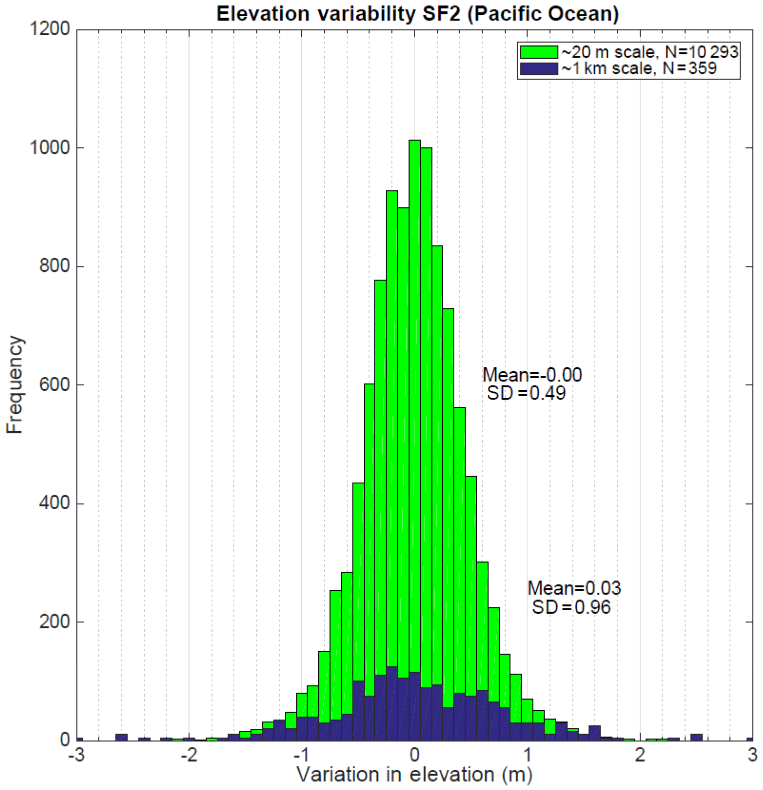
Figure 3 Histogram of the variation in sea surface elevation on the 22 August 2014 ASCENDS flight over the Pacific Ocean near the California coast. The green bars are raw data for every 0.1 s integration time (20 m scale along track), and the blue bars are averages over 5 s (1 km scale along track).

In order to improve precision, the raw lidar measurements may be aggregated to a larger scale before being used for XCO₂ retrievals. The range to the scattering surfaces may vary significantly within the aggregated scale, depending on the roughness of scattering surface and data aggregation time. In previous measurements (Abshire et al., 2013), the standard deviation of range measurements from the aircraft to a flat surface, e.g., Railroad Valley, NV, was about 1 m but increased to 25 m over mountains within a 10 s data average time, which corresponds to 2 km ground track length. These changes are caused by changes in surface topography within the averaging time.

In this study, we first calculated surface elevation for ground and/or cloud tops using lidar range measurements, pointing angle and aircraft altitude. The measurements showed the relative surface elevation change from one data point to the next increases with flight distance. During a flight in the 2014 campaign, one flight was made over the Pacific Ocean near the California coastline with low winds. The lidar range measurements made at 10 Hz show 0.5 m standard deviation in the relative surface elevation changes, as shown in Fig. 3. The standard deviation of the relative surface elevation changes increased to about 1 m after measurements were averaged over 5 s or 1 km horizontal distance. Although the data aggregation before retrieval can increase SNR and improve retrieval precision for flat surfaces, over rougher surfaces like mountains there can be more variation in the photon path length, which can limit the data averaging time before retrieval. Since surface roughness and XCO₂ variations are smaller over ocean than over land, data can be averaged over a longer time over oceans before retrieval.

The elevations of cloud tops can vary significantly. Lidar measurements showed the standard deviation of marine stratus cloud top heights from the 2014 flights at the California coastline was approximately 5 m for a 0.1 s averaging time and increased to 18 m for 5 s averages, as shown in Fig. 4, which is reasonably consistent with estimates from the 2011 flights over the Pacific Ocean (Abshire et al., 2013). As expected, the range measurements to puffy popcorn-like cumulus cloud tops made in the 2014 campaign showed more variation. The standard deviation of the relative cumulus cloud top height changes from one point to the next was 42 m for 0.1 s averages and 107 m for 5 s averages, as shown in Fig. 5. Thus, the partial-column XCO₂ measurements made to cumulus cloud tops using 10 s averaged data are expected to be noisier than these over marine stratus clouds.

Figure 4 The same as Fig. 3 but for the 20 August 2014 flight above marine stratus clouds along the California coastline, showing a 0.1 s standard deviation of 5.2 m and a 5 s standard deviation of 18 m for cloud top height changes from one point to the next.

2.3 Cloud reflectance

The lidar measurement of backscatter profiles also allows us to estimate the reflectance of the scattering surfaces. For a pulsed lidar, the reflectance of a scattering surface is given by

$$\begin{array}{}\text{(1)}& r_s={\displaystyle \frac{E_r}{E_{\mathrm{tr}}}}{\displaystyle \frac{R^{\mathrm{2}}}{{\mathit{\tau }}_{\mathrm{sys}}}},\end{array}$$

where E_r is the signal backscatter pulse energy, E_tr is the laser transmitter energy, R is the range to the surface and τ_sys is the lidar system transmission. The lidar signal from an elevated surface such as an aerosol or a cloud layer only includes the backscattered component from the laser. For the pulsed CO₂ Sounder, only the photons backscattered by clouds within the 150 m thick atmospheric layer (with the 1 µs laser pulse width) are collected and then used to estimate cloud reflectance. In contrast for clouds illuminated by sunlight, a passive sensor viewing the clouds collects all photons including those scattered from outside of the field of view, as well as photons scattered forward by cloud particles and then backscattered by lower clouds. Thus, for thick clouds more sunlight is returned, and the passively measured cloud reflectance is much higher at these wavelengths.

Figure 1 shows an example of airborne lidar measurements and the relative strength of pulse echoes reflected from the ground, cumulus clouds and cirrus clouds. The echoes from the ground show the sharpest vertical profile as the ground is a solid surface. The vertical extent of backscatter from cirrus clouds is broader than those from cumulus cloud tops. This is because cirrus clouds were semi-transparent while cumulus clouds were denser so that only photons reflected back from the cloud tops are scattered back to the receiver. For cumulus clouds, the peak pulse return at offline wavelengths (in red) was about 40 % of the ground return, while for cirrus clouds the peak return was approximately 25 % of ground return.

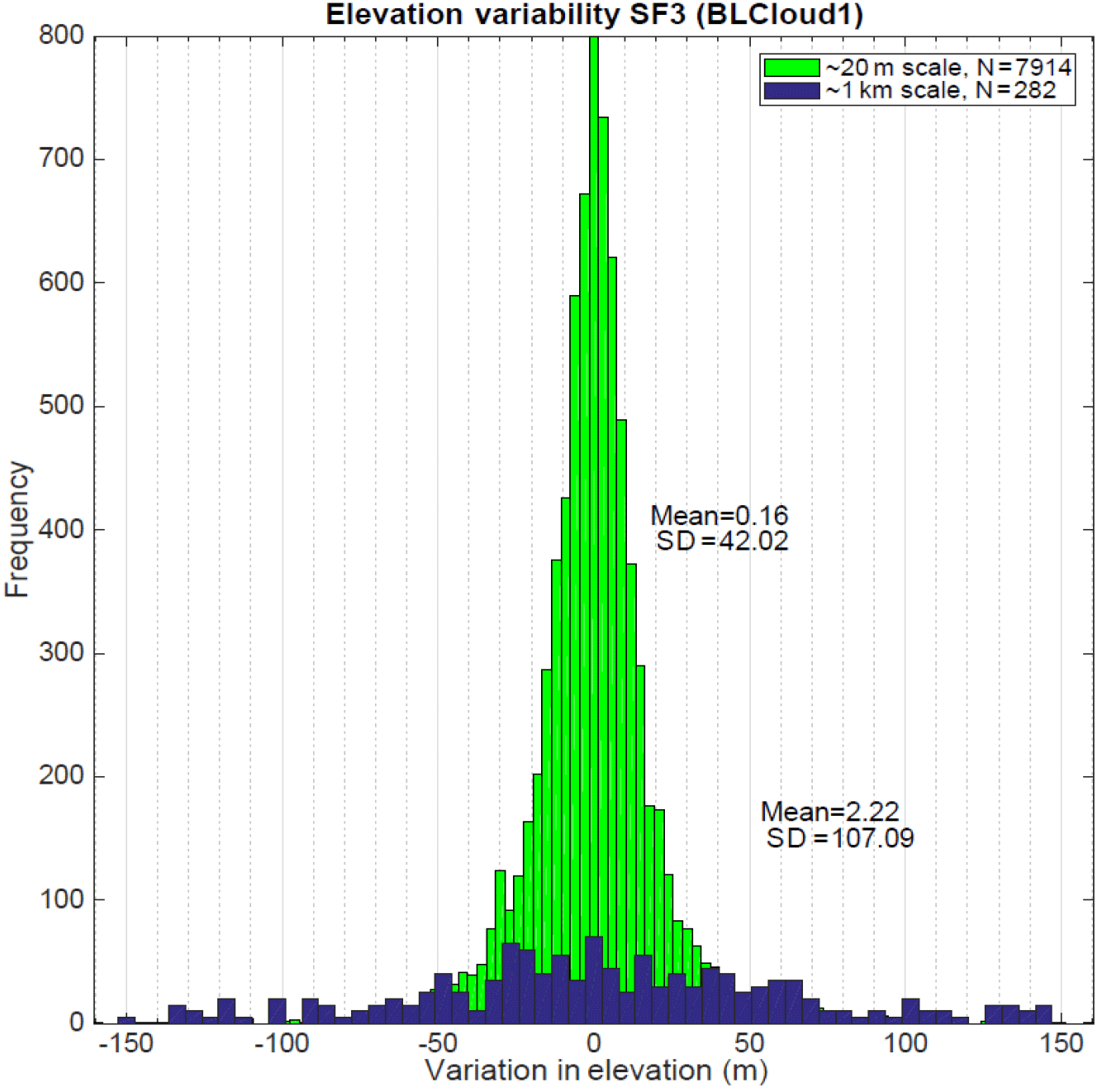
Figure 5 The same as Fig. 4 but for the 25 August 2014 flight above cumulus clouds in Iowa, showing a 0.1 s standard deviation of 42 m and a 5 s standard deviation of 107 m for cloud top height changes from one point to the next.

The lidar-measured cloud top reflectance values were calculated for each flight of these campaigns. Figure 6 shows that for the cumulus clouds over Iowa in 2014, after being averaged in 150 m vertical layers and over 10 s of ground track, the median value of cloud top reflectance was approximately 5 %. The averaged reflectance of Pacific marine stratus cloud tops during the 2011 and 2014 flights was about 4 %. The reflectance of the dense and tall cumulonimbus clouds during a thunderstorm on a 2014 flight in Iowa was slightly higher, 6 %, while the ground reflectance was estimated to be 20 %. The range-resolved reflectance of the cirrus clouds was found to be substantially lower, depending on the physical and spatial structure of the clouds. As shown in the backscatter vertical profiles in Fig. 1, after lidar range correction, reflectance of relatively dense and thick cirrus cloud on the bottom left panel (22:40:04 UTC) was half of cumulus cloud reflectance, or 2–3 %, while reflectance of the thinner cirrus clouds on the right panel (23:00:24 UTC) was 1 %. For the range-distributed backscatter from cirrus clouds, if the vertical signal accumulating layer is increased, then the integrated pulse echo energy and reflectance would be higher.

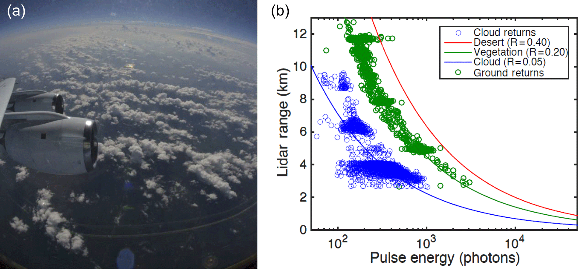
Figure 6 (a) shows the cumulus clouds in the PBL from the ASCENDS sunset flight on 25 August 2014 near the West Branch, Iowa, tall tower. (b) shows the returned pulse energy in number of photons as a function of lidar range from aircraft altitude for the cumulus clouds. The average ground reflectance (in green) is approximately 20 %, while the average cumulus cloud top reflectance is about 5 % (in blue) and shows more variability.

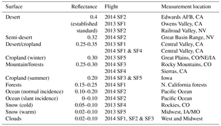
Data analysis shows that the pulsed lidar signals from cloud tops were sufficient to clearly capture the CO₂ absorption line shape. The full line shape from the total of 30 wavelengths across the line is shown in Fig. 2. With the lidar range measurement, this allows quality retrievals of XCO₂ to cloud tops. These retrievals are expected to be noisier than those to the ground due to the lower reflectance of clouds. During the 2013 and 2014 campaigns in the United States West and Midwest, the ground reflectance was 15–40 % (listed in Table 1). Meanwhile, the reflectance of ocean surface at nadir was 10–20 %, depending on wind speed, and quickly dropped to nearly zero when the aircraft banked and the laser pointed off-nadir. Snow ice particles have a strong absorption band near 1500 nm, and snow surfaces have reflectance of 2–10 % at 1572 nm wavelengths, depending on snow condition, e.g., grain size (Wiscombe and Warren, 1980; Painter and Dozier, 2004). In the campaign, snow scenes were sometimes mixed with other more highly reflecting objects, e.g., trees and rocks. Note reflectance of 40 % over desert surfaces is an established standard for estimating reflectance and is very close to in situ measurements made by the GOSAT validation team in Railroad Valley at CO₂ Sounder measurement wavelengths (Kuze et al., 2011).

Table 1 Lidar measurements of surface reflectance during the 2013 and 2014 ASCENDS science flights (SF) over a variety of surface types, including ocean, snow and clouds. Reflectance of 0.4 over desert was specified as a standard to quantify reflectance over other surface types.

3 Cloud identification and data processing

3.1 Cloud identification

Clouds often occur in multiple layers and have variability in density or opacity and cloud top height. Figure 7 shows the shape of the laser pulses transmitted and those backscattered from clouds. The cloud-returned pulse shape varied with cloud type and structure. For the analysis used here, the data processing of cloud returns is performed in two steps. In the first step, pulse echoes from significant scattering surfaces are identified from the lidar backscatter profiles. For hard (ground) or relatively opaque surfaces (dense cloud tops), as shown in Fig. 7, the echo width is limited to 150 m, corresponding to the laser's 1 µs pulse width. For signals backscattered from diffuse clouds, we first subdivided the backscatter profiles into 500 m atmospheric layers. We then labeled those with sufficient backscatter as a pulse echo. The range to each echo was then calculated using the centroid of the backscatter from that layer, as illustrated in Fig. 2. In the second step, the cloud echoes were grouped and stratified for every 500 m layer and then aggregated and averaged over 10 s of ground track. The averaged line shapes were used to retrieve XCO₂ to the averaged centroid cloud height.

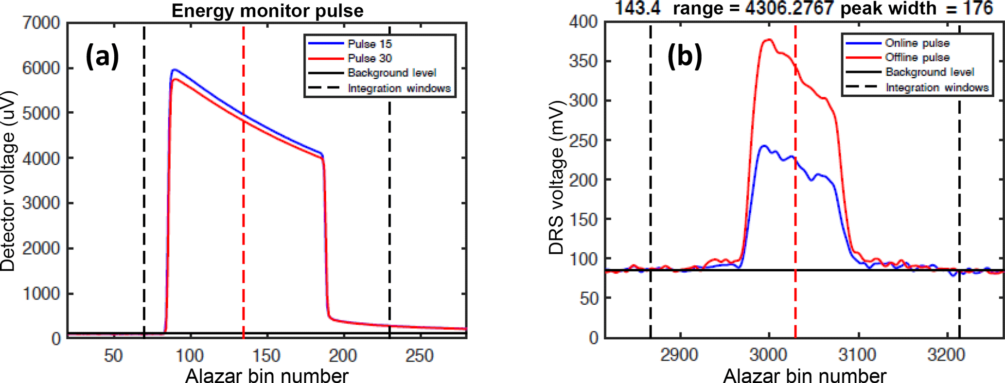
Figure 7 The lidar-transmitted pulse shape (a) and the recorded echo pulse shape returned from a dense cloud top (b). The solid blue lines are for pulse #15, which is near the CO₂ absorption line center, and the solid red lines are for pulse #30, which is in the line wing. Horizontal black lines are signal baselines, and vertical dashed lines indicate signal integration windows. The dashed red lines in the middle are the integration center position in defining the centroid cloud height. Range unit is meters.

The altitude of a significant scattering surface can usually be determined using lidar range, the aircraft GPS altitude and pitch and roll angles. However, during aircraft rolls and turns, distinguishing the altitude of cloud tops from the ground sometimes required using the simultaneous aircraft radar data that provided the nadir range to the ground through the clouds. We also did not data when the aircraft was too close to cloud tops (< 1 km) and when the aircraft tilted substantially (> 10^∘ off-nadir).

3.2 Data processing

The lidar's retrieval process for XCO₂ used several steps. The data from the CO₂ Sounder are calibrated before XCO₂ is retrieved by using a line-fitting retrieval algorithm (Abshire et al., 2014). The calibration utilizes a laser energy vs. wavelength correction (< 10 %); a correction for the transmissions of the receiver's optical band-pass filter (< 2 %); and, for these flights, a detector nonlinearity correction (< 2 %). The laser wavelengths are benchmarked in the lab and field by using auxiliary equipment and measurements. The CO₂ Sounder pulse energy monitor is calibrated while the instrument is operating in the field. The outgoing laser pulse energies are monitored using a beam pick-off, integrating sphere and detector. The acquisition of outgoing pulse energy uses the same digitizer as the lidar backscatter. Additional post-flight calibration is made using a flight segment during the engineering flight with known atmospheric conditions and a high-resolution CO₂ mixing ratio profile measured by an onboard in situ sensor, where instrument parameters are calibrated against atmospheric radiative transfer calculations. This allows assessing the corrections for detector nonlinearity and the receiver's optical band-pass filter. These calibrations are then applied to all retrievals for the science flights.

In the forward calculations, we used the spectroscopy database HITRAN 2008 (Rothman et al., 2009) and the Line-By-Line Radiative Transfer Model (LBLRTM; Clough et al., 1992; Clough and Iacono, 1995) V12.1 to calculate CO₂ optical depth and create look-up tables (LUTs) for a vertically uniform CO₂ concentration of 400 ppm. We then use these LUTs to retrieve the best-fit CO₂ concentration by comparing the measured line shape samples with calculated absorption line shapes. The retrievals used atmosphere (pressure, temperature and water vapor profiles) from the near real time forward processing data of the Goddard Earth Observing System Model, Version 5 (GEOS-5; Rienecker et al., 2011). Data on the full model grid (0.25^∘ latitude × 0.3125^∘ longitude×72 vertical layers, every 3 h) were interpolated to flight ground track position and time for the atmospheric CO₂ absorption calculations. Absorption line fitting was performed in optical depth with a linear least-squares fitting approach. The fitting residuals were spectrally weighted by the square of estimated SNR at each measurement wavelength based on our lidar noise model, which gives more weighting to measurements on line wings than those on line center. The retrieval algorithm solves for Doppler shift, baseline offset, slope, surface reflectance, column-averaged CO₂ and H₂O (XCO₂ and XH₂O) simultaneously for the best fitting. Details of forward calculations and retrieval algorithm were given in Abshire et al. (2014).

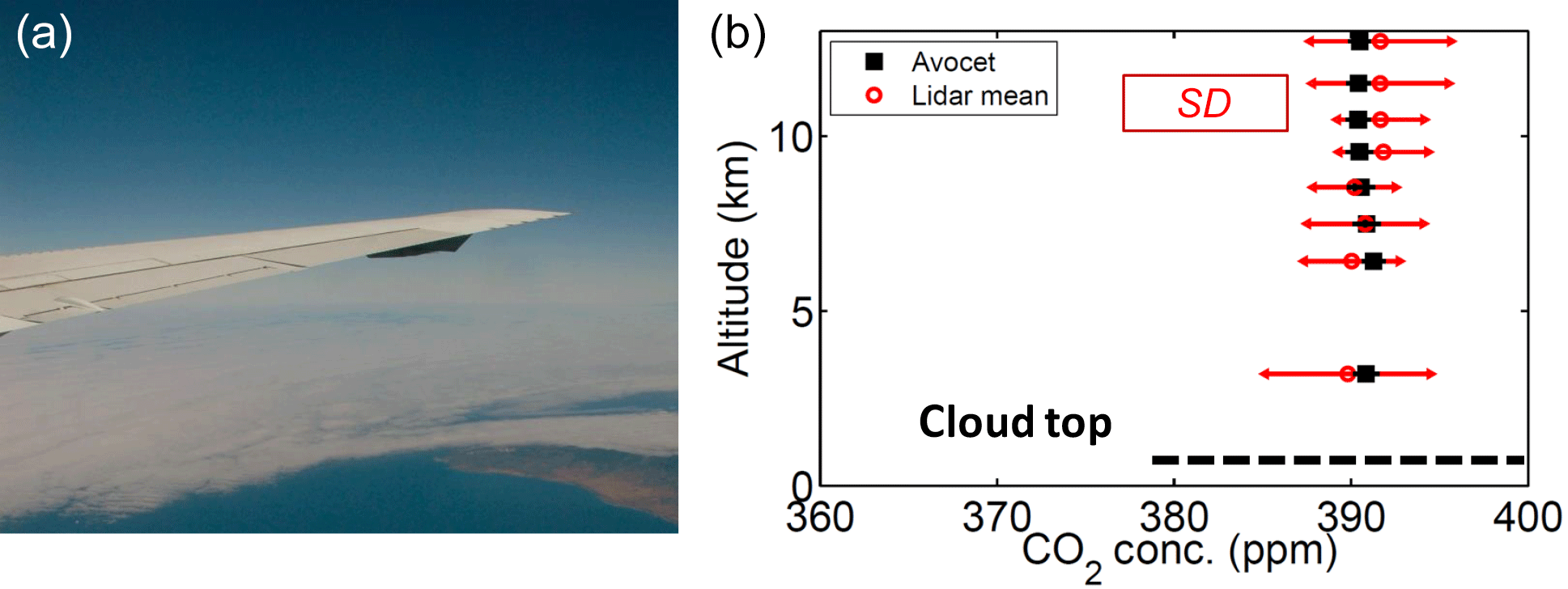
Figure 8 (a) Photo of marine stratus cloud deck over the Pacific Ocean near the California coastline taken on the ASCENDS flight on 2 August 2011. (b) The retrieved values of XCO₂ to the cloud tops at altitudes of 700 m (black dashed line) as a function of flight altitude. The XCO₂ values integrated from the in situ AVOCET gas analyzer are marked in black squares, and the retrieved values from the CO₂ Sounder for 10 s average are marked in red circles. The error bars for the retrieved XCO₂ are for ±1 standard deviation.

There is a weak isotopic water vapor (HDO) line centered at 1572.253 nm on the shoulder of the 1572.335 nm CO₂ line. Depending on atmospheric water vapor content, this can distort the CO₂ line shape and impact the value of the XCO₂ retrieval. The CO₂ Sounder's wavelength assignments place one or two laser wavelengths on the HDO line peak. This allows the retrievals to also solve for XH₂O, which is important because atmospheric water vapor content is highly variable in space and time. Passive remote sensing of greenhouse gases, e.g., OCO-2, GOSAT and TCCON, measures O₂ absorption for column dry-air abundance. Measuring column water vapor is an alternative way to adjust water vapor data from weather forecast models for better estimates of greenhouse gas mixing ratios. This approach has been recommended in the white paper report of NASA's ASCENDS mission (Jucks et al., 2015, http://cce.nasa.gov/ascends_2015/index.html).

4 XCO₂ measurements to cloud tops

During the ASCENDS airborne campaigns in the summers of 2011 and 2014 and the winter of 2013, the CO₂ Sounder made measurements to cloud tops over the US West and Midwest. Retrievals of partial-column XCO₂ were made over low-level marine stratus clouds, cumulus clouds at the top of the PBL with cumulonimbus during thunderstorms, mid-level altocumulus and visually thin cirrus clouds.

4.1 XCO₂ measurements to the tops of marine stratus cloud

Marine stratus clouds exist over a large portion of the ocean adjacent to the west side of continents where ocean currents are cold and a temperature inversion layer is formed to condense the upward-moving moist air. Marine stratus clouds are sheet-like clouds with a nearly horizontally uniform base and top and shallow in depth. Once formed, they may be advected by the wind over land areas. The 2011 ASCENDS airborne campaign had one flight over the Pacific Ocean west of the California coastline on 2 August and flew over marine stratus cloud decks (shown in the left of Fig. 8) with a cloud top elevation of approximately 700 m. The campaign also utilized the Atmospheric Vertical Observation of CO₂ in the Earth's Troposphere gas analyzer (AVOCET; Vay et al., 2011) on board for all flights to measure in situ CO₂ concentration every 1 s. During spiral-down maneuvers, the AVOCET measured the vertical profile of CO₂ concentration. These were used to compare to XCO₂ retrievals from the CO₂ Sounder lidar. The spiral-down maneuvers typically lasted less than 30 min.

The retrieval results are shown in Fig. 8. The right panel shows that the partial-column XCO₂ retrievals based on a 10 s average have 2–4 ppm standard deviation with biases less than 1 ppm over all flight altitudes, compared to the in situ data from the AVOCET. The retrievals with highest precision were from flight altitudes of 8–10 km, indicating the optimal operating altitude for the lidar. At higher altitudes there were fewer returned laser photons and noisier signals, while at lower altitudes the path lengths were shorter and absorption signals weaker. Overall, the retrievals results are comparable in quality to those from other 2011 flights under clear conditions (Abshire et al., 2014).

4.2 XCO₂ measurements to the tops of cumulus cloud

Cumulus clouds form as water vapor condenses in a strong, upward air current above the Earth's surface. Cumulus clouds are often seen over land in the afternoon during summertime after the land surface is fully heated by the Sun. Cumulus clouds usually have flat bases but lumpy tops. Cumulus clouds grow upward and can develop into a tower-like cumulonimbus, which is a thunderstorm cloud.

The 10 August 2011 flight of the ASCENDS airborne campaign flew to Iowa near the West Branch, Iowa, (WBI) tall tower. The flight passed over many isolated cumulus clouds in the area with cloud tops ranging from 1950 to 2200 m near the top of the PBL. Analysis of pulse echoes from both the cloud tops and the ground within the 100 s data averaging time allows solving for the partial-column XCO₂ in the PBL by using the differential absorption line shape. The results showed a strong seasonal drawdown over a cornfield in the area and were consistent with the in situ AVOCET data (Ramanathan et al., 2015).

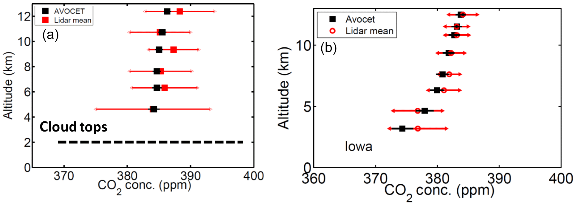
Figure 9 The XCO₂ retrievals for lidar measurements to the tops of broken cumulus clouds (a) and to the ground (b) on the 10 August 2011 ASCENDS flight over Iowa. The XCO₂ values from the in situ AVOCET gas analyzer are marked in black squares, and the values of XCO₂ retrievals from CO₂ Sounder measurements averaged over 10 s are marked in red circles with error bars of ±1 standard deviation. The average altitude of cloud tops (∼ 2 km) is plotted in the dashed line.

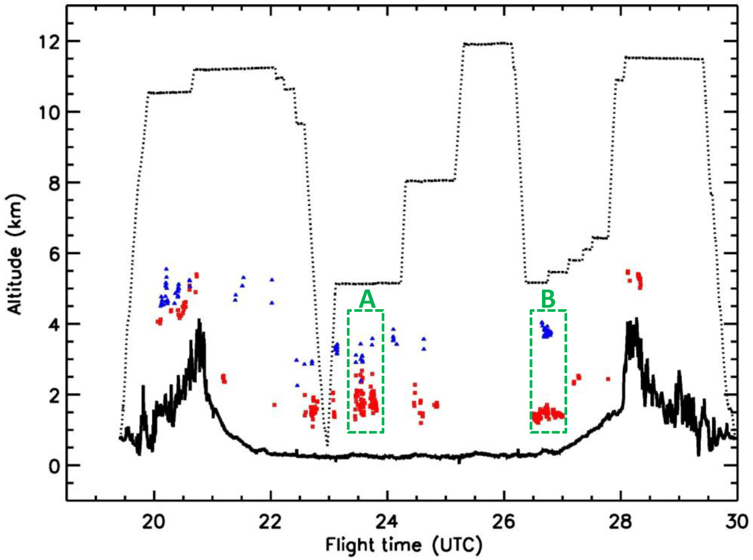
Figure 10 Summary plot of altitude-resolved lidar measurements for the sunset ASCENDS flight to Iowa on 25 August 2014. The aircraft altitude is plotted as the dotted black line, the ground elevation is plotted as the solid black line, the altitudes of boundary layer cloud tops are plotted as the red squares and the altitudes of mid-altitude clouds tops are plotted as the blue triangles. Green boxes “A” and “B” are two segments selected for further data analysis.

For this work, we performed XCO₂ retrievals to the puffy cloud tops for the same flight but use 10 s averaged data as shown in Fig. 2. Retrievals made to the cumulus cloud tops near the spiral-down segment at the West Branch tall tower had standard deviations of 3–6 ppm with average biases less than 1 ppm (Fig. 9, left panel), except for the lowest altitude, where the cloud tops were closer and data became noisier. These statistics are based on retrievals within the spiral-down flight segment with limited sample size, depending on cloud conditions.

Retrievals of XCO₂ to the ground in the same segment showed results with standard deviations of 2–4 ppm and with similar biases, shown in the right panel of Fig. 9. A significant decrease in XCO₂ was evident at lower flight altitudes, caused by the large CO₂ drawdown in the boundary layer above the cornfield. In this region, the cumulus clouds act as a divider to separate free-tropospheric CO₂ from the boundary layer CO₂, which are involved in different physical processes. The difference between the two XCO₂ amounts allows for better estimates of surface sources and sinks (Ramanathan et al., 2015).

During the ASCENDS sunset flight from California to Iowa and back on 25 August 2014, there were many cumulus clouds as shown in Fig. 6. Figure 10 illustrates the detected boundary layer clouds with cloud tops below 2 km and the mid-level clouds with cloud tops around 4 km above ground. In the middle of the flight, a cold front moved through the area, and cumulonimbus clouds developed vertically and a thunderstorm was formed in the region. The cloud top heights ranged from 2 km for PBL cumulus to as high as 3.5 km for cumulonimbus clouds, and the standard deviation of cloud top height was more than 100 m as shown in Fig. 5. The measurement analysis showed the average cloud reflectance was about 6 %, which is sufficient to clearly show the gas absorption features across the measurement line and enable quality retrievals of partial-column XCO₂ to the cloud tops.

We show two segments during the flight to illustrate how XCO₂ retrievals to cloud tops may be used to help resolve horizontal and vertical gradients of atmospheric CO₂ concentration. Both segments have longer than 5 min continuous cloud covers and have more than 30 retrievals to cloud tops for statistics. Segment A, marked in Fig. 10, is a 7 min long segment (23:42–23:49 UTC) near the WBI tall tower during level flight at an altitude of 5 km, while segment B is a 30 min long segment (02:30–03:00 UTC) at a similar altitude on the way back to California after three flights in a square pattern around the WBI tall tower. Most of the clouds in segment A were PBL cumulus clouds that had cloud tops around 2 km above ground. Some were higher cumulonimbus with cloud tops as high as 3.5 km. In segment B most clouds were cumulus with slightly lower tops around 1.5 km, and some were patchy altocumulus clouds with tops around 4 km, which can be clearly seen in Fig. 11. These cloud covers and types can be also identified from photos taken by a digital camera on board.

Over the 7 min segment A with a total of 40 retrievals the lidar measurements of XCO₂ to PBL cumulus cloud tops over a 10 s average had a small bias of 0.2 ppm (395.2 ppm vs. 395.4 ppm of AVOCET) and a standard deviation of 1.94 ppm. The XCO₂ retrievals to the PBL cumulus cloud tops from the lidar measurements in the 30 min long segment B had a standard deviation of 1.85 ppm from a total of 114 retrievals and a mean value of 393 ppm, which is 2.2 ppm lower than those in segment A.

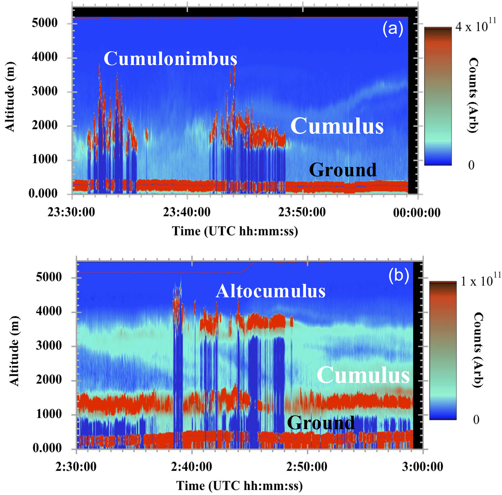
Figure 11 Vertical cross sections of range-corrected backscattered pulse energy for segment A and B marked in Fig. 10. The lidar returns from the ground are at the bottom, and cloud returns are at a variety of altitudes from 1 to 4 km. The red lines on the top of plots indicate aircraft flight altitudes.

The central location of segment B is about 250 km west of segment A. Unfortunately there were no in situ vertical profile data with which to validate this significant gradient. In this situation, CO₂ concentration simulations from the Parameterized Chemical Transport Model (PCTM; Kawa et al., 2004, 2010) were used for intercomparison. PCTM CO₂ concentration simulation is driven by meteorological data from the Modern-Era Retrospective analysis for Research and Applications (MERRA) (Bosilovich, 2013), which is a NASA reanalysis using GEOS-5. The vertical mixing profile in PCTM is parameterized for both turbulence diffusion in the boundary layer and convection. PCTM in this case is run at 1.25^∘ longitude × 1.0^∘ latitude with 56 hybrid vertical levels and outputs hourly, which should be sufficient to resolve the gradient between these two locations, which are 2.4^∘ longitude away, and measurements are 3 h apart.

Figure 12 shows the vertical profile of model CO₂ for both segments. Segment A had high CO₂ concentration in the lower atmosphere. We infer this was likely due to the mixing during the thunderstorm and subsequent surface emission in the evening. The vertical profile in segment B shows a typical summer nighttime vertical structure of CO₂ concentration in the area with overall low value in the lower atmosphere after daytime uptake by growing vegetation but high values near the surface when surface uptake stops and respiration starts. The difference in lidar measurements of XCO₂ to cloud tops by the lidar between segment A and B reflects these two different processes and is consistent with PCTM model simulations. Our XCO₂ retrievals to mid-level cloud tops in the middle of segment B (02:38–02:48 UTC) were back to a high value of 395.8 ppm, on average from 39 retrievals, which excludes the lower CO₂ concentration below clouds. During the same 10 min portion of the segment, our lidar measurements of XCO₂ to PBL cumulus cloud tops stayed at 393 ppm, averaged over 28 retrievals. We had 32 clear-sky full-column XCO₂ retrievals to the ground between the popcorn clouds during the 30 min segment. The average value of full-column XCO₂ was 389 ppm, which is about 4 ppm lower than XCO₂ to cumulus cloud tops and 7 ppm lower than that to the mid-level cloud tops, as illustrated in Fig. 12. The XCO₂ measurements to the land surface had a standard deviation of 1.61 ppm, which, as expected, was less than those to the cloud tops. In this case, the lidar measurements of XCO₂ to cloud tops allow us to distinguish both horizontal and vertical gradients of atmospheric CO₂ concentration.

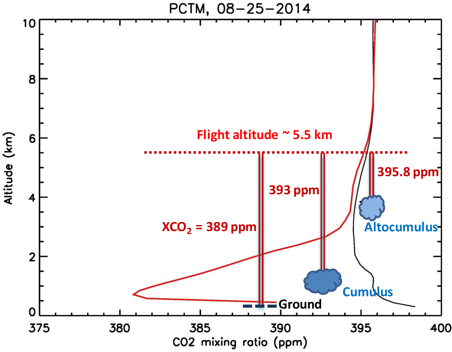
Figure 12 Vertical profiles of CO₂ mixing ratio on 25 August 2014 for the central location of segment A at 41.1^∘ N, 92.3^∘ W in black and of segment B at 41.3^∘ N, 94.7^∘ W in red from the NASA Parameterized Chemical Transport Model. The XCO₂ measurements to ground, PBL cumulus clouds and mid-altitude altocumulus clouds from the CO₂ Sounder lidar for segment B are labeled. Flight altitudes were around 5.5 km above sea level for both segments, shown as a red dashed line.

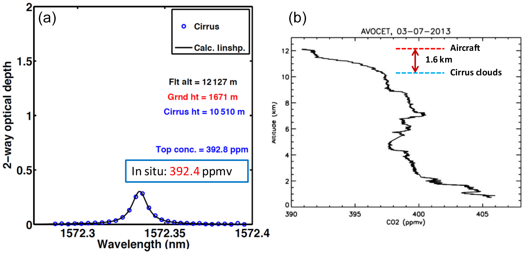
Figure 13 A CO₂ absorption line shape measured on 7 March 2013 to cirrus cloud tops at 10.5 km altitude (a). The lidar measurements are the blue circles, and the fitted line shape is the solid black line. AVOCET in situ vertical profile of CO₂ concentration is plotted in (b). The aircraft flight altitude was 12.1 km, and the lidar range to cirrus cloud tops was 1.6 km.

4.3 XCO₂ measurements to cirrus clouds

Cirrus clouds are thin and semi-transparent clouds, and are globally widespread in the upper troposphere. Cirrus cloud height decreases with latitude, following the tropopause height, and can be as low as 6–8 km at high latitudes and as high as 16–18 km in the tropics (Sassen et al., 2008). The occurrence frequency of cirrus clouds is about 17 % (Sassen et al., 2008) on a global average, but it can be as high as 70 % (Nazaryan et al., 2008) in the equatorial west-central Pacific Ocean, associated with deep convections at the Intertropical Convergence Zone (ITCZ) and seasonal monsoon circulations. Cirrus clouds are composed of ice crystals and strongly absorptive in our CO₂ measurement line (Wiscombe and Warren, 1980; Warren, 1984; Gosse et al., 1995). Therefore, the laser backscatter from cirrus clouds is expected to be substantially lower than from clouds composed of water droplets. The reflectance of cirrus clouds varies with cloud physical and spatial structure.

Some cirrus clouds encountered during the ASCENDS airborne campaigns were dense and thick and had sufficient echo pulse energy to show clear CO₂ absorption line shape. However, for most cases, the energy values were lower, and the absorption line shapes are not sufficiently clear to allow quality retrievals. Figure 13 shows an example of XCO₂ retrievals to cirrus cloud tops near the spiral-down flight segment in Iowa on 7 March 2013. The data are averaged over 100 s and show a clear CO₂ absorption line shape. The aircraft altitude was 12.1 km, and the averaged cirrus cloud top height was 10.5 km. The lidar measurements show a retrieval of XCO₂ of 392.8 ppm to the cirrus cloud tops, which is lower than the full-column XCO₂ to the ground of 398 ppm. The lidar retrieval is consistent with in situ AVOCET data of 392.4 ppm for the same layer average in the stratosphere. Unfortunately, there were not enough cases with suitable cirrus cloud tops during these three campaigns to allow calculation of statistics.

5 Discussion and conclusion

The pulsed multi-wavelength IPDA lidar approach allows accurate determination of the photon path lengths and accurate retrieval of XCO₂ to cloud tops. Measurements to cloud tops and ground were made with the CO₂ Sounder lidar during the 2011, 2013 and 2014 ASCENDS airborne campaigns. These measurements were used to study the XCO₂ retrievals made to a variety of cloud tops and to demonstrate the value of these retrievals in resolving both horizontal and vertical gradients of atmospheric CO₂. Measurements were made over a variety of clouds, including cumulus and marine stratus at the top of the boundary layer, mid-level altocumulus and cirrus. For all clouds except cirrus, the data processing rate was greater than 90 %, excluding cases when the aircraft was too close to cloud tops and when the aircraft tilted substantially.

Analysis of the airborne campaign measurements showed that the laser pulse energies from the tops of boundary layer clouds such as stratus and cumulus were usually sufficient to allow clear identification of CO₂ absorption line shape and good retrievals of partial-column XCO₂ to cloud tops. On average, the reflectance of the boundary layer cloud tops was 5 %. In most cases, the boundary layer clouds are too thick for laser pulse to penetrate and allow ground echoes to return simultaneously. However, over broken clouds, after averaging over 10 s of ground track or longer, both cloud and ground returns were available. If clouds are patchy or broken, retrievals of both XCO₂ to the ground and to cloud tops simultaneously and the difference between the two could be then used to estimate the residual XCO₂ in the boundary layer, whose value is the most sensitive to surface carbon sources and sinks.

For passive remote-sensing approaches, cirrus clouds can significantly modify the photon path length and cause a significant error in XCO₂ retrievals. In contrast, the lidar measurements showed range-resolved pulse echoes from semi-transparent cirrus clouds and the ground. In some cases those could be used to retrieve full-column XCO₂ to the ground and partial-column XCO₂ to cirrus and then to estimate tropospheric column XCO₂. However, in most cases during the campaigns, the backscattered pulse energies from cirrus clouds were low, compared to other clouds such as stratus and cumulus clouds. Only dense and thick (> 1.0 km) cirrus clouds allowed detection of clear CO₂ absorption line shapes and thus yield good XCO₂ retrievals. One limitation for these initial airborne measurements was that cirrus clouds were at high altitude (∼ 10 km) so that the column path length from aircraft altitudes to the cloud tops was short and the CO₂ absorption signal was weak. For future space-based missions, the path length of pulse echoes from cirrus clouds will be longer and the CO₂ absorption will be stronger, improving retrievals.

The quality of the CO₂ Sounder retrievals is being improved with advancing technologies for the laser and detector, toward the measurement goals of ASCENDS. Our results show that XCO₂ retrievals to the flat marine stratus cloud tops have the same quality as those to the sea surface. That is probably because the higher homogeneity of cloud reflectivity compensates well for the lower cloud reflectivity at the measurement wavelengths and makes the SNRs for returns from both the clouds and the surface almost identical (Amediek et al., 2017). Meanwhile, when compared to in situ data with sufficient samples (> 30), the XCO₂ retrievals to the puffy cumulus cloud tops near the West Branch tall tower in Iowa showed low bias (∼ 0.2 ppm) and standard deviation of 1.9 ppm. In this case, the standard deviation of XCO₂ retrievals to the cumulus cloud tops were increased by 20 %, compared to the standard deviation of 1.6 ppm for the retrievals to the ground, mainly due to the larger cloud top roughness as well as the lower cloud reflectivity at the measurement wavelengths. Previous ASCENDS observing system simulation experiments (OSSEs) with clear-sky measurements (Kawa et al., 2010; Hammerling et al., 2015) have shown that lidar approaches have greater spatial and temporal coverage than passive approaches and hence a higher potential to reduce uncertainties in carbon budget estimates. Retrievals to all-level cloud tops with corresponding measurement precision are planned to be included in future OSSE studies to assess their impact on atmospheric transport modeling and surface flux estimates.

Partial-column XCO₂ retrievals to different cloud tops and to the ground allow us to distinguish horizontal and vertical gradients of atmospheric CO₂. This measurement capability for the future space carbon missions will be particularly valuable for the regions with persistent cloud covers. These include tropical ITCZ, west coasts of continents with marine layer clouds, and the Southern Ocean with the highest occurrence of low-level clouds, where underneath carbon cycles are active but where measurements from passive satellite-based spectrometers are limited. Lidar-based measurements to cloud tops will fill these significant gaps, provide a more complete picture of the CO₂ distribution and benefit atmospheric transport modeling as well as global and regional carbon budget estimates.