Error sources in the retrieval of aerosol information over bright surfaces from satellite measurements in the oxygen A band

Retrieving aerosol optical thickness and aerosol layer height over a bright surface from measured top-of-atmosphere reflectance spectrum in the oxygen A band is known to be challenging, often resulting in large errors. In certain atmospheric conditions and viewing geometries, a loss of sensitivity to aerosol optical thickness has been reported in the literature. This loss of sensitivity has been attributed to a phenomenon known as critical surface albedo regime, which is a range of surface albedos for which the top-of-atmosphere reflectance has minimal sensitivity to aerosol optical thickness. This paper extends the concept of critical surface albedo for aerosol layer height retrievals in the oxygen A band, and discusses its implications. The underlying physics are introduced by analysing the top-of-atmosphere reflectance spectrum as a sum of atmospheric path contribution and surface contribution, obtained using a radiative transfer model. Furthermore, error analysis of an aerosol layer height retrieval algorithm is conducted over dark and bright surfaces to show the dependence on surface reflectance. The analysis shows that the derivative with respect to aerosol layer height of the atmospheric path contribution to the top-of-atmosphere reflectance is opposite in sign to that of the surface contribution – an increase in surface brightness results in a decrease in information content. In the case of aerosol optical thickness, these derivatives are anti-correlated, leading to large retrieval errors in high surface albedo regimes. The consequence of this anti-correlation is demonstrated with measured spectra in the oxygen A band from the GOME-2 instrument on board the Metop-A satellite over the 2010 Russian wildfires incident.

1 Introduction

Aerosols are one of the largest sources of uncertainties in our understanding of the Earth's current climate and its future projection, because of the role they play in complex atmospheric processes that influence the Earth's radiation budget (IPCC, 2014). More generally, aerosols influence the climate either directly through absorption and scattering of solar radiation, or indirectly through cloud formation and aerosol–cloud interaction.

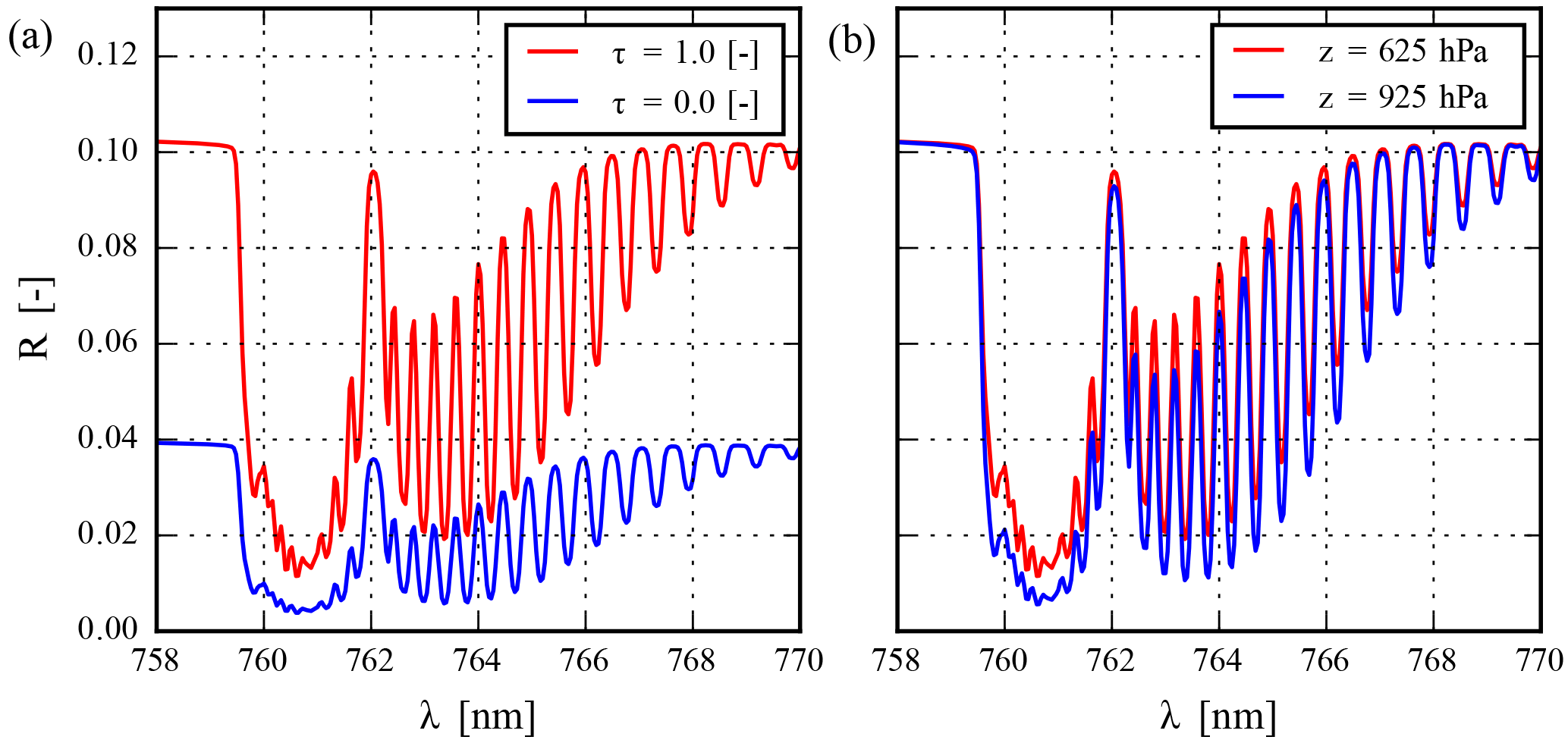
Figure 1 Synthetic oxygen A-band spectra for a cloudless atmosphere containing aerosols over a surface with an albedo of 0.03, as measured by a nadir pointing instrument for a solar zenith angle at 45^∘. The instrument settings are that of the UVN instrument. Aerosol single-scattering albedo is fixed at 0.95 and scattering by aerosols is described by a Henyey–Greenstein phase function with an asymmetry factor (g) of 0.7. (a) Aerosol layer is fixed at a height of 900–950 hPa, for two scenes are different aerosol optical thicknesses. (b) Aerosol vertical distribution is varied for an aerosol optical thickness of 1.0 at 760 nm.

In climate studies, the direct radiative effect of aerosols is calculated to understand its net contribution to the Earth's total radiation budget. This depends on aerosol macrophysics (such as vertical distribution) and microphysics (such as size distribution and single-scattering albedo), which determine whether aerosols in a particular scenario are more efficient in absorbing or scattering the incoming solar radiation and the thermal radiation from within the Earth's atmosphere. The ability of aerosols to absorb radiation can influence thermal stability of the atmosphere, which in turn influences cloud formation and atmospheric chemistry (IPCC, 2014; Chung and Zhang, 2004). Knowledge of the vertical distribution on aerosols is, hence, an important piece of the puzzle to reduce uncertainties in our understanding of Earth's climate. Because of the high degree of variability of aerosols in both time and space, this knowledge is required at a high spatio-temporal resolution.

To observe (among other atmospheric parameters) aerosols, many space-borne Earth observation initiatives have been proposed to monitor the Earth's atmosphere with either active or passive remote sensing techniques. An example of such an initiative is the Cloud-Aerosol LIdar with Orthogonal Polarization (CALIOP) instrument on board NASA's Cloud-Aerosol Lidar and Infrared Pathfinder Satellite Observations (CALIPSO) mission, which provides information on the vertical distribution of aerosols. However, because of the limited swath of a space-borne lidar instrument, the mission coverage area is also limited. This gap in the data can be filled with satellite missions carrying passive remote sensing instruments, which have a larger coverage area with good temporal resolution. One such initiative is the Copernicus programme by the European Commission (EC) partnered with ESA, which aims to provide accurate information of atmospheric composition from space. Of its missions, the Sentinel-5 Precursor, Sentinel-5 and Sentinel-4 are examples of polar-orbiting and geostationary satellites equipped with hyperspectral sensors (Veefkind et al., 2012; Ingmann et al., 2012).

Hyperspectral instruments on board the Sentinel-4/5/5P missions measure Earth radiance and solar irradiance in the top of atmosphere, spectrally resolved over a wide wavelength range. Of the wavelength bands measured, these instruments also measure in the oxygen A band between 758 and 770 nm, where absorption of solar radiation is dominated by molecular oxygen and its isotopologues. The presence of aerosols in the atmosphere significantly impacts absorption of solar radiation by molecular oxygen (Fig. 1a). In the absence of clouds and aerosols, the oxygen A band can either be almost transparent or opaque to solar radiation, owing to the large variation in the absorption cross section within the spectra. In the presence of an aerosol layer in the atmosphere, the absorption intensity of the spectra can provide useful vertical information (as observed in Fig. 1b) – deeper absorption lines correspond to a lower aerosol layer, and shallow absorption lines to a higher aerosol layer. This is the basis of retrieving aerosol layer height from the oxygen A band. Currently, the Copernicus Sentinel-4/5/5-P aerosol layer height algorithms are designed to exploit oxygen absorption spectra in the A band to retrieve the height of an aerosol layer.

The retrieval of aerosol properties from the oxygen A band presents a few challenges, one of them being that aerosol layers in the atmosphere are usually optically thin, and are quite difficult to observe in the presence of clouds. This is because clouds have an optical depth which is typically orders of magnitude larger than that of aerosols, and are more efficient in scattering incoming radiation. Consequently, aerosol retrieval algorithms generally refrain from retrieving over cloudy scenes; our algorithm is no exception to this and requires cloud screening to filter out pixels containing clouds.

While cloudy pixels can be filtered out to a certain degree, retrieving aerosols from measurements in the oxygen A band over bright surfaces faces a host of other challenges. From the literature, it is understood that aerosol information content from measured spectra in the oxygen A band reduces as the surface albedo increases (Corradini and Cervino, 2006; Sanghavi et al., 2012). Sanders et al. (2015) report potentially large biases in their aerosol layer height retrievals from the oxygen A band when the surface albedo is fitted. In a previous paper, Sanders and de Haan (2013) also report that certain specific combinations of geometry, aerosol, and surface properties can result in unusually large uncertainties in the retrieved aerosol layer height (see also Fig. 8-2 in Sanders and de Haan, 2016). Such large biases can perhaps be attributed to a phenomenon known as the critical surface albedo regime (Seidel and Popp, 2012), wherein for specific surface albedos, the top-of-atmosphere reflectance becomes independent of the aerosol optical thickness. Sanders et al. (2015) observe that when the surface albedo is not fitted, typical uncertainties in the surface albedo database over land can result in large biases. From our analyses, we understand that for relative errors up to 10 % in the surface albedo, retrievals over dark surfaces are not affected, whereas the same over sufficiently bright surfaces (surface albedo greater than 0.2) can suffer from very large biases.

A combination of all the error sources discussed previously can result in large biases. In fact, we observe that the presence of errors often leads to no convergence in the retrieval, with no concrete predictability on which pixel is likely to yield no result. Because of this, the operational algorithm wastes resources trying to retrieve aerosol layer height from pixels that potentially do not have any usable aerosol information. This is especially problematic in the framework of high-resolution instruments, which demand operational processors to make efficient use of computational time and effort to process large number of spectra (typically several hundred per second). In order to design more efficient operational algorithms, the concept of critical surface albedo needs to be extended beyond the framework provided by Seidel and Popp (2012) into the oxygen A band for aerosol optical thickness as well as aerosol layer height.

This paper analyses simulated measured top-of-atmosphere reflectance spectra in the oxygen A band and provides an explanation for the loss of aerosol information over bright surfaces. Its implication is provided in an optimal estimation framework, specific to the retrieval of aerosol layer height, with results from sensitivity analyses. The analysis is followed up with a demonstration in a real data environment by retrieving aerosol layer height over a bright surface. The case study chosen is the retrieval of optically thick biomass-burning aerosol plumes over the 2010 Russian wildfires, to demonstrate the effect of this loss of aerosol information over land. This paper is one in a series of papers on development of an operational oxygen A-band Aerosol Layer Height retrieval algorithm for Sentinel-4/5/5-P by KNMI, preceded by Sanders and de Haan (2013) and Sanders et al. (2015). The current operational ALH algorithm for S5P is described in Sanders and de Haan (2016). While the results of this paper are relevant for the Sentinel 5-Precursor algorithm as well, the instrument model used in the sensitivity studies is for the UVN spectrometer on the S4 mission.

The next section (Sect. 2) provides a description of the forward model and the optimal estimation framework. Section 3 discusses the concept of aerosol–surface ambiguities in the oxygen A band. Section 4 describes various sensitivities of our retrieval algorithm focusing on the difference between dark and bright surfaces. Section 5 discusses aerosol layer height retrievals over the 2010 Russian wildfires using GOME-2A data. Section 6 concludes this paper with a discussion and the implication of the findings from this paper.

2 The forward model and the inverse method

2.1 Forward model

There are three primary parts of the forward model, namely the atmospheric model, the radiative transfer code, and the instrument model. A radiative transfer code is used to model a high-resolution top-of-atmosphere radiance by propagating radiation through the atmosphere described by the atmospheric model. The top of atmosphere reflectance R computed by the forward model is defined as the ratio of the radiance I of the pixel measured by the instrument to the top-of-atmosphere solar irradiance E₀ of the pixel on a horizontal surface unit,

$$\begin{array}{}\text{(1)}& {\displaystyle }{\displaystyle }R\left(\mathit{\lambda }\right)={\displaystyle \frac{\mathit{\pi }I\left(\mathit{\lambda }\right)}{{\mathit{\mu }}_{\mathrm{0}}{E}_{\mathrm{0}}\left(\mathit{\lambda }\right)}},\end{array}$$

where μ₀ represents the cosine of the solar zenith angle of the pixel, and λ represents the wavelength.

The top-of-atmosphere reflectance is calculated after the measured radiance and irradiance are convolved with the instrument spectral response function (ISRF) of the hyperspectral sensor in order to simulate measured spectra by a satellite instrument. For simulations, the high-resolution solar spectrum from Chance and Kurucz (2010) is used.

2.1.1 Radiative transfer model

The radiative transfer model is the layer-based orders of scattering (LABOS) method, which is a variant derived from the doubling-adding method (de Haan et al., 1987). Atmospheric properties are calculated line-by-line to compute the reflectance at the top of atmosphere. The radiative transfer code is a part of a software package called DISAMAR (Determining Instrument Specifications and Analysing Methods for Atmospheric Retrievals), which is the main workhorse of the operational algorithm development efforts at KNMI for oxygen A-band aerosol height retrieval with S5P/S4/S5 instruments. Scattering by gases is described by Rayleigh scattering, which has a low scattering cross section in this wavelength region. Because of this, polarization is ignored. Wavelength shifts caused by rotational Raman scattering (RRS) are ignored in order to reduce computational effort, since line-by-line calculations are computationally expensive in the oxygen A band. This is convenient, since the Raman scattering cross section is even smaller than that of Rayleigh scattering. The atmosphere in the forward model is plane-parallel for the Earth radiance, and spherically corrected for the incoming solar irradiance.

2.1.2 Atmospheric model

For cloud-free conditions, the following four absorption and scattering processes are significant in the wavelength range between 758 and 770 nm: scattering by gases, reflection of light by the surface, scattering and absorption by aerosol particles, and absorption by molecular oxygen. Absorption of solar radiation by O₃ and H₂O are ignored, since they are not dominant absorbing gases in this spectral range.

The surface reflectance is assumed isotropic, described by its albedo. Depending on the surface albedo, a surface can either be bright or dark. Dark surfaces are classified with surface albedo close to 0.05 (or lower), which in the oxygen A-band spectral region typically corresponds to ocean surfaces. Bright surfaces in the oxygen A band on the other hand have a surface albedo of 0.2 (intermediately bright) and higher and are primarily over land. For the oxygen A band at 760 nm, typical values of surface albedo over vegetated surfaces exceed 0.4 since the wavelength band is located beyond the red edge, where absorption of solar radiation by chlorophyll diminishes. Scenes with snow or ice are not processed.

Aerosols are represented as a single layer with a fixed pressure thickness of 50 hPa, containing aerosol particles with a fixed aerosol optical thickness and aerosol single-scattering albedo. Aerosol layer height is defined as the mid-pressure of the aerosol layer – if the aerosol layer extends from 650 to 600 hPa, the aerosol layer height is 625 hPa. In the operational S5P aerosol layer height algorithm, currently the aerosol phase function is a Henyey–Greenstein model (Henyey and Greenstein, 1941) with an asymmetry factor of 0.7, and an aerosol single-scattering albedo of 0.95 (Sanders et al., 2015). While a Mie scattering model could be used instead of the Henyey–Greenstein model, the latter is computationally less expensive and hence more optimal for the operational algorithm.

Oxygen absorption cross sections are derived from the NASA JPL database, following Tran and Hartmann (2008) who indicate that line parameters in the JPL database are more accurate than the HITRAN 2008 database. First-order line mixing and collision-induced absorption by O₂–O₂ and O₂–N₂ are derived from Tran et al. (2006) and Tran and Hartmann (2008).

2.1.3 Instrument model

The instrument model is described by the instrument slit function, whose spectral resolution depends on its full width at half maximum (FWHM), and its noise model. For this study, oxygen A band is simulated using specifications of the Sentinel-4 Ultraviolet Visible and Near-infrared (UVN) instrument, which is set to launch in 2022. The instrument is a sounder with a hourly coverage over Europe and northern Africa at a spatial resolution of 8 km × 8 km sampled at 45^∘ N and 0^∘ E. The instrument has a FWHM of approximately 0.116 nm, oversampled by a factor of 3, effectively giving the instrument a spectral sampling interval of 0.04 nm. Aerosol layer height will be an operational product provided by the Sentinel-4 mission. An example of oxygen A-band spectra at a 0.116 nm resolution is provided in Fig. 1. For retrievals with real data, measurements from the Global Ozone Monitoring Experiment-2 on board the MetOp-A satellite are used. Launched on 16 October 2006, GOME-2A is an optical spectrometer fed by a scanning mirror, which enables across-track scanning in the nadir. The instrument has a spectral sampling interval of approximately 0.21 nm at 758 nm (spectral resolution of 0.48 nm for channel 4), and has a nominal spatial resolution of 80  km× 40 km (Munro et al., 2016). A shot noise model is assumed for the instrument.

2.2 Inverse method

The inverse method is based on the optimal estimation (OE) framework described by Rodgers (2000), which is a maximum a posteriori (MAP) estimator that constrains the least-squares solution with a priori knowledge on the state vector. The method assumes Gaussian statistics for the a priori errors. The iterative method is a Gauss–Newton approach, and the estimation parameters are the aerosol optical thickness τ and the aerosol layer height z. The cost function χ² is defined as

$$\begin{array}{ll}{\displaystyle }{\mathit{\chi }}^{\mathrm{2}}=& {\displaystyle }[\mathit{y}-\mathit{F}\mathbf{(}\mathit{x}\mathbf{,}\mathit{b}\mathbf{\left)}{]}^T{\mathbf{S}}_{\mathit{ϵ}}^{-\mathrm{1}}\right[\mathit{y}-\mathit{F}\mathbf{(}\mathit{x}\mathbf{,}\mathit{b}\mathbf{)}]\\ \text{(2)}& {\displaystyle }& {\displaystyle }+(\mathit{x}-{\mathit{x}}_{\mathrm{a}}{)}^T{\mathbf{S}}_{\mathrm{a}}^{-\mathrm{1}}(\mathit{x}-{\mathit{x}}_{\mathrm{a}}),\end{array}$$

where y is the measured reflectance, F(x,b) is the vector of calculated reflectance using the forward model, x is the state vector containing fit parameters, b is the vector containing other model parameters, S_ϵ is the measurement error covariance matrix, x_a is the a priori state vector, and S_a is the a priori error covariance matrix. S_a is diagonal, assuming no correlation between state vector elements. S_ϵ is also diagonal, since the measurement error is assumed uncorrelated. $[\mathit{y}-\mathit{F}\mathbf{(}\mathit{x}\mathbf{,}\mathit{b}\mathbf{\left)}{]}^T{\mathbf{S}}_{\mathit{ϵ}}^{-\mathrm{1}}\right[\mathit{y}-\mathit{F}\mathbf{(}\mathit{x}\mathbf{,}\mathit{b}\mathbf{)}]$ is the measurement part of the cost function, whereas $(\mathit{x}-{\mathit{x}}_{\mathrm{a}}{)}^T{\mathbf{S}}_{\mathrm{a}}^{-\mathrm{1}}(\mathit{x}-{\mathit{x}}_{\mathrm{a}})$ is the state vector part of the cost function.

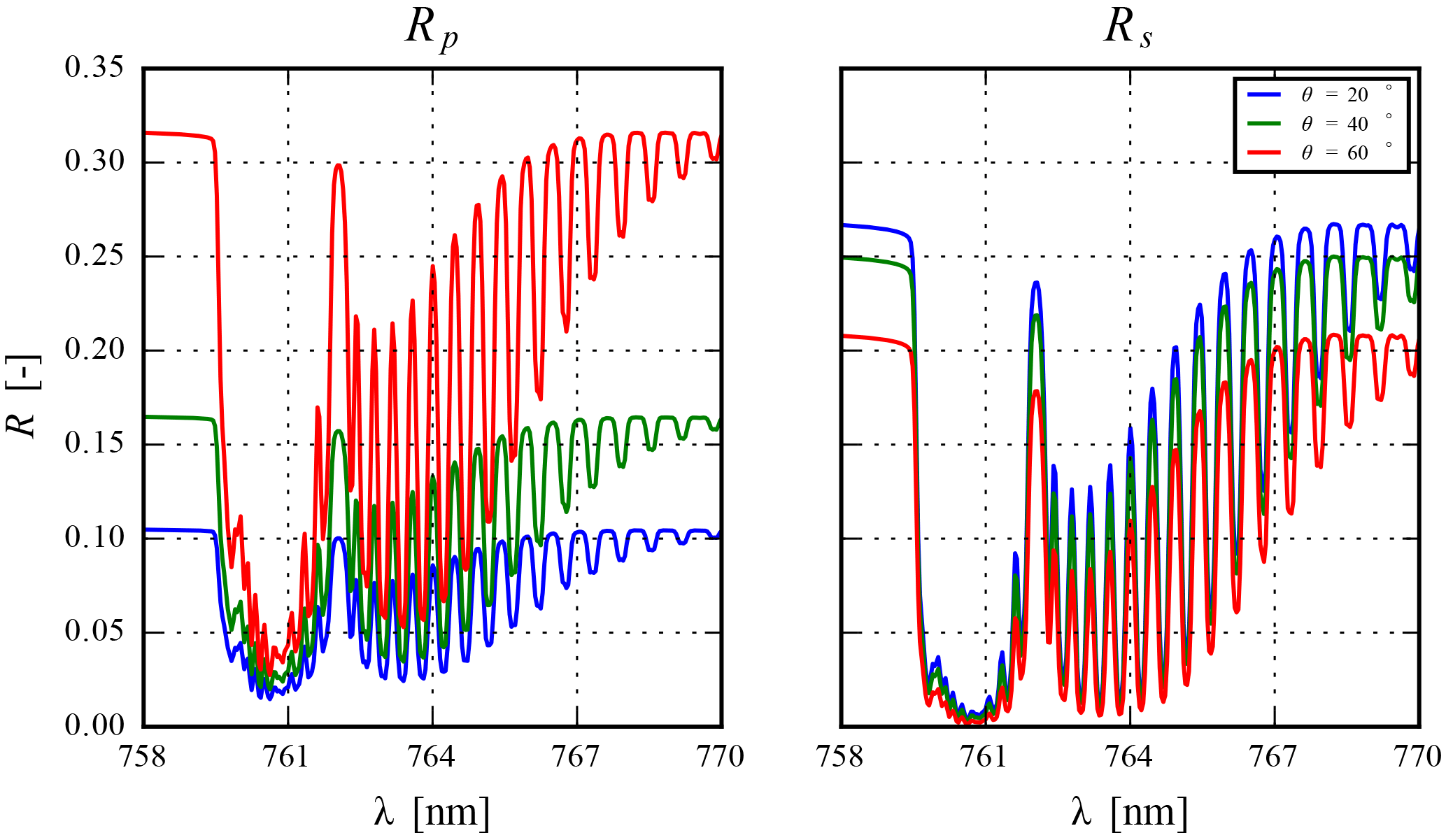
Figure 2 R_p and R_s for increasing viewing zenith angle θ over a surface with an albedo of 0.4 at 760 nm. The solar zenith angle is fixed at 45^∘ and a relative azimuth angle of 0^∘. Aerosol optical thickness is fixed at 1.0 for an aerosol single-scattering albedo of 0.95. Aerosol scattering phase function is a Henyey–Greenstein with g=0.7. The aerosol layer is situated at 600 hPa, with a thickness of 50 hPa.

The a posteriori error covariance matrix $\widehat{\mathbf{S}}$ is computed as

$$\begin{array}{}\text{(3)}& {\displaystyle }{\displaystyle }\widehat{\mathbf{S}}=({\mathbf{K}}^T{\mathbf{S}}_{\mathit{ϵ}}\mathbf{K}+{\mathbf{S}}_{\mathrm{a}}^{-\mathrm{1}}{)}^{-\mathrm{1}},\end{array}$$

where K is the Jacobian with its columns containing partial derivatives of the reflectance with respect to the state vector elements. DISAMAR calculates the Jacobian semi-analytically, similar to the reciprocity method described by Landgraf et al. (2001). The Jacobian drives the retrieval towards the solution as an integral component in the update to the state vector,

$$\begin{array}{ll}{\displaystyle }{\mathit{x}}_{n+\mathrm{1}}=& {\displaystyle }{\mathit{x}}_{\mathrm{a}}+({\mathbf{K}}_n^T{\mathbf{S}}_{\mathit{ϵ}}^{-\mathrm{1}}{\mathbf{K}}_n+{\mathbf{S}}_{\mathrm{a}}^{-\mathrm{1}}{)}^{-\mathrm{1}}{\mathbf{K}}_n^T{\mathbf{S}}_{\mathit{ϵ}}^{-\mathrm{1}}[\mathit{y}-\mathit{F}\left({\mathit{x}}_n\right)\\ \text{(4)}& {\displaystyle }& {\displaystyle }+{\mathbf{K}}_n({\mathit{x}}_n-{\mathit{x}}_{\mathrm{a}})],\end{array}$$

where x_n+1 is the next iteration to the nth iteration in the retrieval, and K_n is the Jacobian evaluated at the nth iteration. The Jacobian can become singular if the value of the partial derivative of the reflectance to the state vector parameter is very low, or is correlated to another parameter in the state vector. In these cases, the error covariance matrix does not exist, since the inverse covariance matrix is non-invertible; if it is nearly singular, the problem is ill-conditioned and may result in very large biases in the estimation.

The inverse method reaches a solution if the change in the state vector between iterations is below a convergence threshold. It is possible that during iterations, the inverse method estimates state vector elements beyond boundaries. In such a case, the state vector element is adjusted back to just within its physical limits. If the adjustment is made in two consecutive iterations, the retrieval is stopped and no solution is reached. The upper cap in the number of iterations is set at 12, beyond which the retrieval is said to have failed. In this paper, these failed retrievals are termed as non-convergences. The next section discusses the atmospheric conditions that can potentially lead to these non-convergences.

3 Aerosol–surface ambiguities in the oxygen A band

3.1 Influence of surface reflectance on aerosol information content in the oxygen A band

The top-of-atmosphere reflectance over a surface with an albedo A_s can be written as the sum of atmospheric path contribution of the photon R_p and surface contribution R_s,

$$\begin{array}{}\text{(5)}& {\displaystyle }{\displaystyle }\mathit{R}(\mathit{\lambda },A_{\mathrm{s}})={\mathit{R}}_{\mathrm{p}}\left(\mathit{\lambda }\right)+{\mathit{R}}_{\mathrm{s}}(\mathit{\lambda },A_{\mathrm{s}}).\end{array}$$

R_p is the top-of-atmosphere reflectance in the absence of a surface. R_s is calculated by subtracting the path contribution from the total top-of-atmosphere reflectance, and represents contributions from photons that have been reflected one or more times by the surface. R_s is dependent on the absorbing and scattering species present in the atmosphere, and also includes aerosol influences. R_p is calculated by substituting A_s=0.0 and calculating the top-of-atmosphere reflectance in DISAMAR. R_s is calculated by subtracting R_p from R. With increasing viewing angle, R_p increases whereas R_s decreases (Fig. 2). This is in line with expectation, since the slant aerosol optical thickness increases, which increases the amount of contribution that aerosols have in R(λ,A_s). At steeper geometries, light at the top of atmosphere is more diffuse than direct, which is the primary reason why R_s decreases (assuming a Lambertian surface).

For a model parameter x with two values x_a and x_b, the difference spectrum ΔR_Δx, defined as

$$\begin{array}{}\text{(6)}& {\displaystyle }{\displaystyle }\mathrm{\Delta }{R}_{\mathrm{\Delta }x}=R_{x_a}-R_{x_b},\end{array}$$

can reveal the influence the model parameter x has on the oxygen A band. The spectral shape of ΔR_Δx can also show parts of the spectrum that are more sensitive to x. Following Eqs. (5) and (6), ΔR_Δx(λ,A_s) is defined as

$$\begin{array}{}\text{(7)}& {\displaystyle }{\displaystyle }\mathrm{\Delta }{R}_{\mathrm{\Delta }x}(\mathit{\lambda },A_{\mathrm{s}})=\mathrm{\Delta }{\mathit{R}}_{{\mathrm{p}}_{\mathrm{\Delta }x}}\left(\mathit{\lambda }\right)+\mathrm{\Delta }{\mathit{R}}_{{\mathrm{s}}_{\mathrm{\Delta }x}}(\mathit{\lambda },A_{\mathrm{s}}).\end{array}$$

If $\mathrm{\Delta }{\mathit{R}}_{{\mathrm{p}}_{\mathrm{\Delta }x}}$ and $\mathrm{\Delta }{\mathit{R}}_{{\mathrm{s}}_{\mathrm{\Delta }x}}$ have opposing signs, ΔR_Δx reduces following Eq. (7), which results in a reduction of sensitivity to the parameter x.

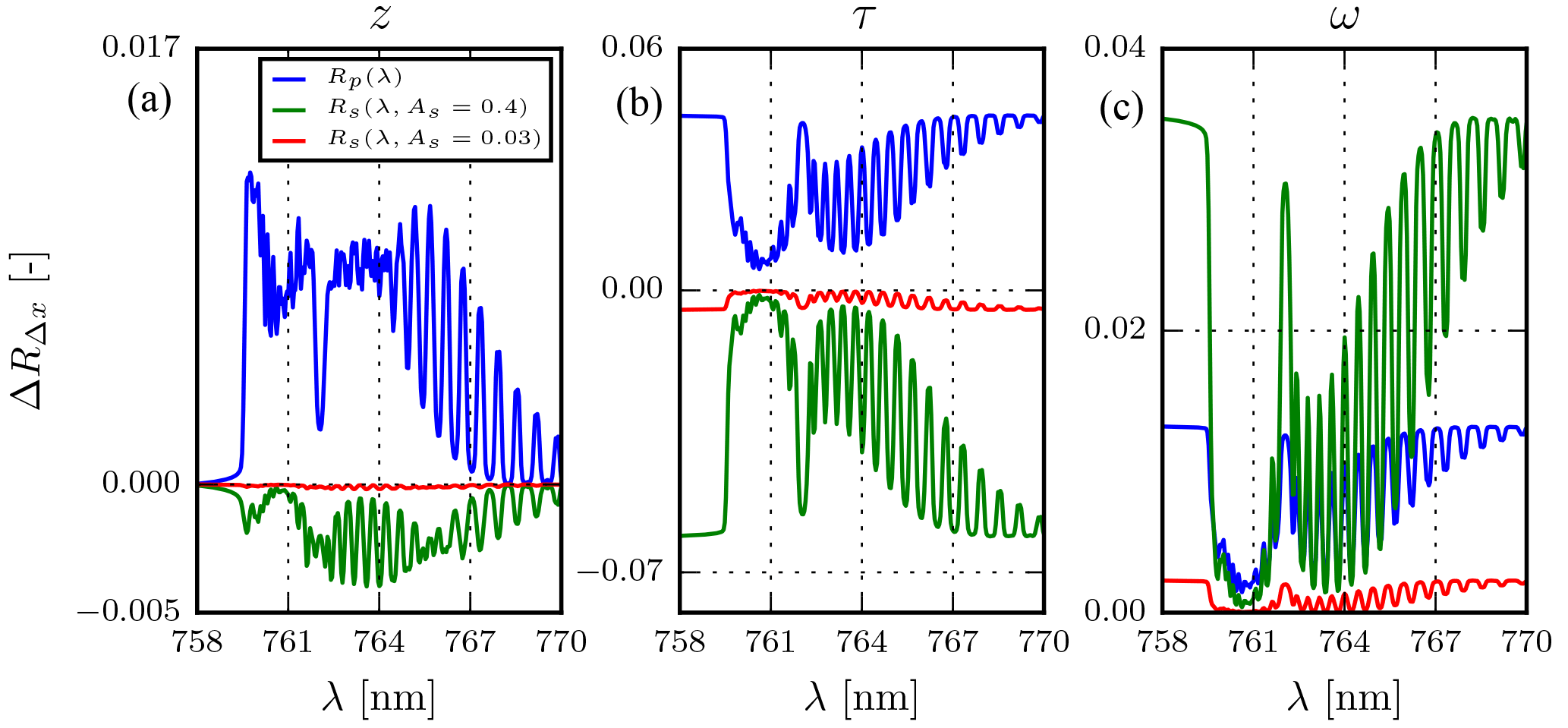
Figure 3 $\mathrm{\Delta }{\mathit{R}}_{{\mathrm{p}}_{\mathrm{\Delta }x}}$ (in blue) and $\mathrm{\Delta }{\mathit{R}}_{{\mathrm{s}}_{\mathrm{\Delta }x}}$ (in red for A_s=0.03 and green for A_s=0.4) to model parameter x in the oxygen A band, as measured by a nadir-pointing instrument for a solar zenith angle at 45^∘. $\mathrm{\Delta }{\mathit{R}}_{{\mathrm{p}}_{\mathrm{\Delta }x}}$ is calculated as the difference of the modelled top-of-atmosphere reflectance between two atmospheres, both cloudless and containing aerosols, which differ only in the parameter x for values x_a and x_b, according to Eq. (6). The phase function is described by a Henyey–Greenstein model with an anisotropy factor of 0.7, and the thickness of the aerosol layer is fixed at 50 hPa. (a) τ=1.0 and ω=0.95 with different aerosol layer heights, z_a=600 hPa and z_b=800 hPa. (b) τ_a=1.0 and τ_b=0.5 at z=600 hPa and ω=0.95. (c) τ=1.0 and z=600 hPa for ω_a=0.95 and ω_b=0.9. The Y axis has been optimized per plot.

Figure 4 Derivative of reflectance with respect to aerosol properties for different surface albedos A_s. The z is centred around 600 hPa, with τ=1.0, ω=0.95, and a Henyey–Greenstein phase function with g=0.7. The solar zenith angle is 45^∘ and the viewing zenith angle is 0^∘. (a) Derivative of reflectance with respect to z. (b) Derivative of reflectance with respect to τ. (c) Derivative of reflectance with respect to ω. The colour bar has been optimized per plot.

Figure 5 Top-of-atmosphere reflectance at 755 nm, well outside the oxygen A band, from simulated spectra of scenes containing aerosols over dark and bright surfaces. Red, blue, and green lines represent different viewing zenith angles θ, as a function of increasing aerosol optical thickness. Aerosols have a single-scattering albedo of 0.95, and the aerosol scattering is described by a Henyey–Greenstein phase function with g = 0.7. Aerosol layer is situated at 925 hPa. The solar zenith angle is 45^∘ and a relative azimuth angle is 0^∘. (a) The surface albedo is 0.03 at 760 nm, typical over the ocean. (b) The surface albedo is 0.25 at 760 nm, typical over land. (c) The surface albedo is 0.4 at 760 nm, typical over vegetated land.

Comparing $\mathrm{\Delta }{\mathit{R}}_{{\mathrm{p}}_{\mathrm{\Delta }z}}$ and $\mathrm{\Delta }{\mathit{R}}_{{\mathrm{s}}_{\mathrm{\Delta }z}}$ at two different aerosol layer heights (z) for two different scenes with the same atmospheric conditions (Fig. 3a), it is observed that $\mathrm{\Delta }{\mathit{R}}_{{\mathrm{p}}_{\mathrm{\Delta }z}}$ and $\mathrm{\Delta }{\mathit{R}}_{{\mathrm{s}}_{\mathrm{\Delta }z}}$ have opposite signs and R_p is relatively more sensitive to aerosol layer height than R_s. This is especially the case in the deepest part of the R branch between 759.50 and 761.30 nm and parts of the P branch between 761.30 and 763.00 nm, where the higher absorption cross section reduces the number of photons that can reach the surface. This ultimately reduces the magnitude of R_s to the top of atmosphere for these absorption sub-bands. $\mathrm{\Delta }{\mathit{R}}_{{\mathrm{s}}_{\mathrm{\Delta }z}}$ over ocean and vegetation also shows an increase in its overall magnitude with an increase in surface albedo, and hence an increase in cancellation between ΔR_pΔz and ΔR_sΔz. Figure 4 represents the variation of the derivative of reflectance with respect to aerosol properties, for increasing surface albedo. Albeit subtle, the consequence of this cancellation between ΔR_pΔz and ΔR_sΔz is observed in Fig. 4a, where ∂R$/\partial z$ for the deepest part in the R branch and parts of the P branch diminishes gradually with an increase in surface albedo.

The same experiment is repeated for aerosol optical thickness (τ), and the results are presented in Fig. 3b. $\mathrm{\Delta }{\mathit{R}}_{{\mathrm{p}}_{\mathrm{\Delta }\mathit{\tau }}}$ and $\mathrm{\Delta }{\mathit{R}}_{{\mathrm{s}}_{\mathrm{\Delta }\mathit{\tau }}}$ are anti-correlated (Pearson correlation coefficient is −0.99, irrespective of the surface albedo), and the magnitude of $\mathrm{\Delta }{\mathit{R}}_{{\mathrm{s}}_{\mathrm{\Delta }\mathit{\tau }}}$ increases with an increase in surface albedo. Figure 4b shows the partial derivative of the reflectance with respect to τ for increasing surface albedo. This anti-correlation explains negative derivatives in the higher surface albedo regime.

$\mathrm{\Delta }{\mathit{R}}_{{\mathrm{p}}_{\mathrm{\Delta }\mathit{\omega }}}$ and $\mathrm{\Delta }{\mathit{R}}_{{\mathrm{s}}_{\mathrm{\Delta }\mathit{\omega }}}$ of aerosol single-scattering albedo (ω) in Fig. 3c reveals a strong correlation (with a Pearson correlation coefficient of almost unity). This suggests that an increase in surface albedo increases the sensitivity of the model to ω. We suspect that this information predominantly arises from interactions between scattered light by aerosols and surface. The magnitude of the partial derivative of reflectance with respect to ω for increasing surface albedo (shown in Fig. 4c) shows an increase, which is in line with our analysis of Fig. 3c.

For increasing surface albedo, the more dynamic parts of the $\partial \mathit{R}/\partial \mathit{\tau }$ spectrum in Fig. 4b correspond to spectral points with less absorption by molecular oxygen. These are also the parts of the spectrum with a high signal-to-noise ratio (SNR) and high $S_{\mathit{ϵ}}^{-\mathrm{1}}$. From Eq. (4), the inverse method gives a higher priority to spectral points with a higher $S_{\mathit{ϵ}}^{-\mathrm{1}}$. Intuitively, low information of τ from the oxygen A-band spectrum will increase the dependence of the inverse method to prior information. This is further discussed in the next section.

3.2 Aerosol–surface interplay in the top-of-atmosphere reflectance

In the inverse method, an a priori error of 100 % is assumed for the aerosol optical thickness, which gives it freedom to vary during iterations. If the a priori aerosol optical thickness is far from the solution, a large a priori error ensures that the retrieval can estimate the parameter in fewer iterations. However, whether the Gauss–Newton optimization reaches the correct solution depends on two primary factors: first, whether the cost function has a global minimum, and second, whether the gradient of the cost function is sufficiently large such that it is minimized significantly at every iteration.

From our analysis of ΔR_Δx for aerosol parameters, we have identified aerosol optical thickness to be the parameter most affected by an increasing surface albedo, due to the cancellation between $\mathrm{\Delta }{\mathit{R}}_{{\mathrm{p}}_{\mathrm{\Delta }\mathit{\tau }}}$ and $\mathrm{\Delta }{\mathit{R}}_{{\mathrm{s}}_{\mathrm{\Delta }\mathit{\tau }}}$ owing to their similar amplitudes and spectral shapes (but opposing signs). Because of this, the top-of-atmosphere reflectance spectrum becomes independent of aerosol optical thickness for higher surface albedo regimes (Fig. 5).

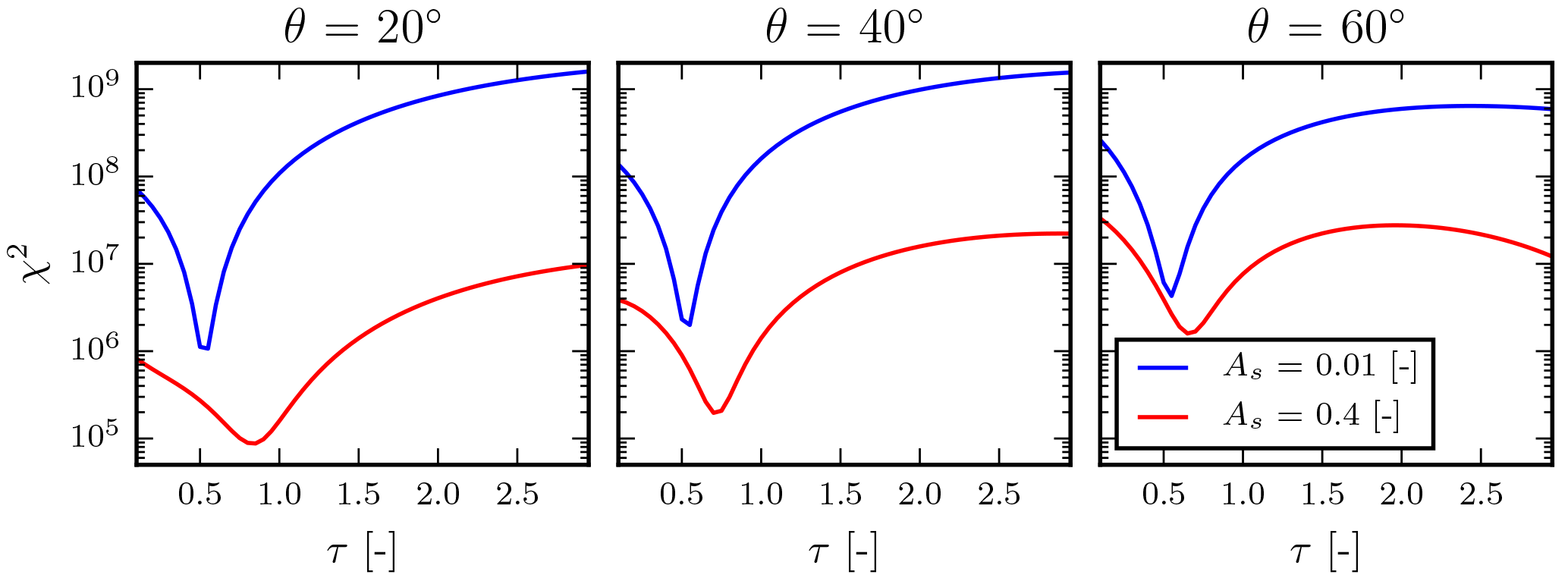
Figure 6 Cost function (χ²) for retrieving aerosol optical thickness as a function of aerosol optical thickness per iteration (τ) for a dark and a bright surface. The true aerosol optical thickness is 0.5, and the aerosol layer is situated at 600 hPa with a 50 hPa layer thickness. The aerosol single-scattering albedo is fixed at 0.95, for a Henyey–Greenstein aerosol phase function with g=0.7. The solar zenith angle is fixed at 45^∘ for varying viewing angles as specified in the plot titles. The relative azimuth angle is 0^∘. The state vector also contains aerosol layer height, whose a priori value is fixed at 700 hPa.

Over a dark surface such as the ocean, top-of-atmosphere reflectance in the continuum is unique at different aerosol loads (Fig. 5a). The variation in the top-of-atmosphere reflectance in the continuum reduces as the instrument points more towards the nadir. In such geometries, R_s can play a more significant role than R_p and reduce the available information on τ in the R(λ,A_s) spectrum. For bright surfaces, the variation in the top-of-atmosphere reflectance spectrum is less for steeper geometries relative to the same geometries over the ocean (Fig. 5b, green and blue lines). There can also be cases where, provided sufficiently high aerosol loading, the top-of-atmosphere reflectance spectrum in the continuum can be independent of aerosol optical thickness over very bright surfaces such as vegetation (Fig. 5c, green line). In such cases, more than one value of τ results in the same top-of-atmosphere reflectance. Henceforth in this paper, this phenomenon is termed as aerosol–surface ambiguity.

A loss in aerosol information can have special implications in the minimization of the cost function. As observed in Fig. 6, for lower surface albedo regimes there exists a single minimum of the cost function. For such scenes, if the a priori aerosol optical thickness is far from the true value, the gradient is sufficiently large such that a small change in the state vector between iterations leads to a significant minimization of the cost function. As the surface albedo increases, this gradient decreases significantly, and can also result in the presence of multiple minima in the cost function (Fig. 6, right) if the state vector is far away from the truth. This makes the retrieval dependent on the initial guess of τ.

Because of a model error (described in Fig. 6) in the aerosol layer height between y and F(x,b) (in Eq. 2), the global minimum of the cost function shifts away from the true τ. This shift is biased higher than the truth if the aerosol layer is lower in the atmosphere in comparison to the aerosol layer in the synthetic true spectrum, because the model has to compensate the extra absorption by molecular oxygen. If the aerosol layer is higher in the atmosphere, the minimum of the cost function is situated at a τ lower than the true τ. As observed in Fig. 6 (left, red line), this shift of the cost function minimum from the true τ is larger over bright surfaces for a viewing angle close to nadir, where R_s is more dominant. For the same angle, the global minimum over a dark surface is situated at the true τ value, even with the presence of a model disagreement with the simulated “true” spectrum. As the viewing angle increases over the bright surface, R_p increases and the global minimum of the cost function moves closer towards the true τ.

If the a priori error assigned to aerosol optical thickness is large, presence of aerosol–surface ambiguities can result in non-convergences. Because the a priori part of the cost function has a smaller value than the measurement part, reducing a priori error assigned to the aerosol optical thickness does not necessarily guarantee a solution to this issue since it does not remove the multiple-minima present in the cost function. Since errors between aerosol optical thickness and aerosol layer height are correlated (Sanders et al., 2015), a large error in the optical thickness will lead to a large error in the aerosol layer height estimate. The next section discusses the sensitivity of the aerosol layer height algorithm to this phenomenon by introducing model errors in a simulation environment.

4 Error analysis

In DISAMAR, forward models for simulation and retrieval have been kept separate so that errors can be introduced into the simulated spectra to mimic errors in a real retrieval scenario. In this section, the instrument model of the Sentinel-4 UVN near-infrared spectrometer is used. The wavelength range for simulations and retrievals is between 758 and 770 nm. A comparative analysis of biases in the retrieved aerosol layer height is conducted over ocean (A_s=0.03) and land (A_s=0.25, and A_s=0.4). Bias in the aerosol layer height is defined as the difference between retrieved and true aerosol layer height (in hPa) – a positive sign indicates that the aerosol layer is retrieved below the true aerosol layer height. The aerosol layer height retrieved is a single layer for the entire atmospheric column, with a fixed thickness of 50 hPa.

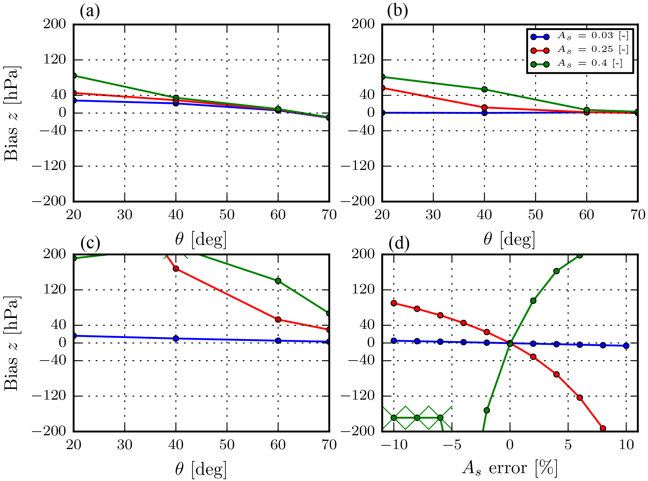
Figure 7 Bias in aerosol layer height in the presence of model errors. Unless specified, the relative azimuth angle is 0^∘ and the solar zenith angle is 45^∘, aerosol single-scattering albedo is 0.95, Henyey–Greenstein g is 0.7, and there is an aerosol layer at 650 hPa. (a) Model error is introduced in the thickness of the aerosol layer. The simulated spectrum contains a 200 hPa thick aerosol plume extending from 1000 to 800 hPa. (b) Model error is introduced in the aerosol phase function. The simulated scenes contain aerosols with scattering physics described by a Henyey–Greenstein phase function with g=0.65 and retrieved with g=0.7. (c) Model error is introduced in the single-scattering albedo. The simulated spectrum contains aerosols with ω=0.95, which is fixed in the retrieval forward model at 0.90. (d) A relative error is introduced in the surface albedo. The viewing angle is fixed at 20^∘.

4.1 Sensitivity to model error in the aerosol layer thickness

In a typical real-world scenario, aerosol plumes can be as thick as 200 hPa in the atmosphere, or more. We simulate a scene containing an aerosol layer that extends approximately from the surface (1000 hPa) to 800 hPa in the atmosphere. The true τ is 1.0, and the a priori τ is 0.5. The a priori value of the aerosol layer height is 650 hPa, and the aerosol layer thickness is fixed at 50 hPa. In an ideal retrieval instance, the retrieved aerosol layer height (which has a thickness of 50 hPa) should coincide with the height of the simulated thicker aerosol layer. We observe that, in general, the error in the retrieved aerosol layer height reduces as the viewing zenith angle increases (Fig. 7a). This is explained by a reduction in R_s and an increase in R_p (Fig. 2, red line), which explains why difference in errors between retrievals over different surfaces reduces with an increase in viewing angle (Fig. 7a, high viewing zenith angles).

At lower viewing zenith angles, the difference in aerosol layer height errors between retrievals over the different surfaces is the largest, since the effect of R_s cancelling out with R_p is significantly larger (Fig. 2, blue line), which increases with an increase in surface albedo (Fig. 3a). The retrieved aerosol layer is biased towards the surface in all three surface albedo scenarios, with the aerosol layer being placed closer to the surface if the surface albedo is brighter. This should not suggest a sensitivity to the geometrical thickness of the aerosol layer. As the surface albedo increases, the number of photons that pass through the atmosphere to interact with the surface before reaching the detector increases. These photons have a longer path length, which results in an increased absorption by oxygen at specific spectral points with weak oxygen absorption lines. In comparison to photons at wavelengths with strong oxygen absorption lines, these photons have a higher SNR since relatively more of them reach the detector. A higher SNR ensures lower noise, and hence a higher value in the inverse of the measurement error covariance matrix S_ϵ. If a spectral point has a higher value in $S_{\mathit{ϵ}}^{-\mathrm{1}}$ matrix, it has a higher representation in the cost function (in Eq. 2), and hence a higher preference (or weight) in the optimal estimation. Because of this, the retrieval prefers to retrieve an aerosol layer height described by photons that travel through the aerosol layer closer to the surface. If, however, the aerosol optical thickness is so large that the photons cannot penetrate the aerosol layer, the retrieved aerosol layer height would be more accurate. Retrieving the height of optically thin aerosol layers can also be quite challenging, owing to the fact that these layers will allow more photons to pass through and interact with the surface, leading to an increase in R_s, and hence an increase in the cancellation between R_p and R_s. As a result of this, large biases in the retrieved aerosol layer height can be expected for optically thin layers over bright surfaces.

Another consequence of retrieving aerosol layer height over bright surfaces is that the retrieval may become more susceptible to model error in aerosol and surface properties, such as the aerosol phase function anisotropy factor g, the aerosol single-scattering albedo ω, and especially the surface albedo A_s, which are fixed in the model. These are investigated in the following.

4.2 Sensitivity to model error in the aerosol phase function

The presence of a model error in the aerosol phase function can result in large biases if the surface is bright (Fig. 7b). For a higher surface brightness and a viewing angle close to nadir, this bias is larger. As the viewing angle increases, the biases reduce significantly. The correlation of bias with surface albedo suggests that biases caused by model errors are exacerbated by the surface contribution R_s, which reduces as viewing angle increases (Fig. 2, right).

4.3 Sensitivity to model error in aerosol single-scattering albedo

From Fig. 4, aerosol single-scattering albedo plays an increasingly significant role in the retrieval of aerosol layer height as the surface gets brighter. Because of this, a mis-characterization of aerosol single-scattering albedo in the model can lead to very large biases over bright surfaces (Fig. 7c), and also non-convergences. This is not the case for retrievals over the ocean, since the influence of aerosol single-scattering albedo on the oxygen A-band spectrum is low. It is observed that, as the viewing angle increases, these biases drop significantly. This is again attributed to the decrease in R_s and increase in R_p with increasing viewing angle (again, over a Lambertian surface).

4.4 Sensitivity to model error in surface albedo

Surface albedo is a critical component in the accurate retrieval of aerosol layer height over bright surfaces. Because it is a fixed parameter in the forward model, an error in the surface albedo can result in large biases in the retrieval. To simulate model errors, relative errors of −10 to 10 % are introduced in the retrieval forward model, such that the surface is modelled darker or brighter than the true value. For relative errors of ±10 %, the retrieved aerosol layer height can be biased more than 2 orders of magnitude larger over land than over ocean (Fig. 7d). For retrievals over a bright surface such as vegetation (A_s=0.4 or greater), the model error can result in non-convergences. As the model error reduces, retrievals over land with a surface albedo of 0.25 become more acceptable. However, over very bright surfaces, an inaccuracy in surface albedo of more than 2 % can result in biases greater than 100 hPa.

The next section demonstrates the implication of these errors in a real retrieval scenario.

5 Demonstration case: 2010 Russian wildfires

The 2010 Russian wildfires began in late July and lasted for several weeks until the beginning of September. Literature reports droughts and record summer temperatures in the same year as a precursor to the wildfires, both of which have been attributed to climate change (Hansen et al., 2012). A consequence of the forest fires were optically thick aerosol plumes over the country, especially over Moscow. In the first few weeks of August 2010, due to the presence of a strong anti-cyclonic circulation pattern in the atmosphere, the impact of biomass-burning aerosols on air quality in Moscow was markedly larger than what was observed from previous wildfire incidences – the ultraviolet aerosol index (UVAI) reported by the Ozone Monitoring Instrument (OMI) on board the NASA Aura mission observed an increase by a factor of 4.1 over previous years (Witte et al., 2011) over Moscow, due to aerosol plumes originating from the south and east of the city.

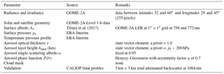
The aerosol plume above Russia on 8 August 2010 serves as a test case for the aerosol layer height retrieval algorithm, due to fairly cloud-free conditions and the optical thickness of the aerosol plume (see Fig. 8c). Because of this, we do not employ a cloud-screening method. The GOME-2A instrument crosses over the scene at approximately 09:45–09:47 local time. The GOME-2A pixels within the region of interest are recorded between 07:45 and 07:48 UTC, at approximate latitude bounds of 52 and 60^∘ and longitude bounds 29 and 45^∘. This corresponds to 255 pixels in total. Meteorological information relevant to the retrieval are temperature–pressure profiles and surface pressure, acquired from the European Centre for Medium-Range Weather Forecast (ECMWF) ERA-Interim database (Dee et al., 2011) at the GOME-2A pixel using nearest-neighbour interpolation. Surface albedo is derived using nearest-neighbour interpolation for version 1.3 of GOME-2A LER climatology derived from Tilstra et al. (2017), which is at a $\mathrm{1}{}^{\circ }\times \mathrm{1}{}^{\circ }$ grid. Typical values of the surface albedo over the region of interest is around 0.21. In the inverse method, the a priori value of the aerosol layer height is approximately 800 hPa. The a priori aerosol optical thickness is 1.0 at 760 nm.

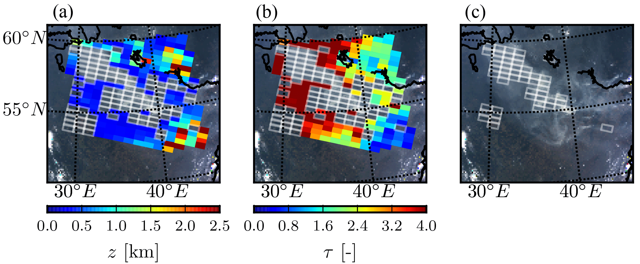
Figure 8 (a) Retrieved aerosol layer height from GOME-2A measurements of the 2010 Russian wildfires, in kilometres above the ground with the aerosol layer height retrieval algorithm. Empty white boxes represent pixels that do not converge to a solution. (b) Retrieved aerosol optical thickness from the same retrievals. (c) GOME-2A pixels for which there exist possible aerosol–surface ambiguities (empty pixels with white borders).

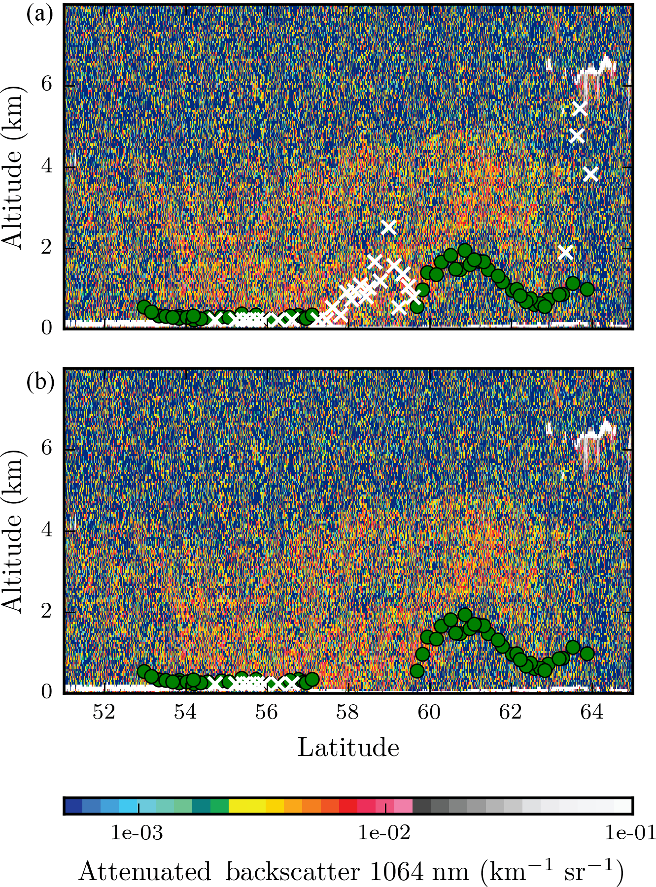
Figure 9 CALIOP lidar backscatter cross section of a track falling within the region of interest over the 2010 Russian wildfire plume on 8 August 2010. (a) Green dots and white crosses are GOME-2A pixels falling within 100 km of the CALIPSO ground track – green dots represent converged aerosol layer heights, and white crosses represent the aerosol layer heights at the last iteration for pixels that do not converge to a solution. These retrieved altitudes are reported in km above ground surface. (b) Retrieval results are presented for pixels for which the prefit method retrieves both ${\mathit{\tau }}_a^{\prime }$ and ${\mathit{\tau }}_b^{\prime }$ at similar values.

CALIOP data are used for validation, which provide vertical distribution of aerosols and clouds for a footprint of approximately 70 m, with a 5 km horizontal resolution (Winker et al., 2009). While the coverage of the instrument is not as expansive as the GOME-2 instrument, the level of information available from CALIOP gives a good idea on the vertical position of aerosols in the atmosphere. For a better validation dataset, CALIOP data recorded between coordinates 52.0^∘ latitude and 64.0^∘ latitude approximately around 10:45 UTC are used for comparison of GOME-2A aerosol layer height retrieval results. The Level-1 CALIOP attenuated backscatter data from 1064 nm is used because lidar in the visible region (532 nm) can get heavily attenuated over optically thick plumes. As can be seen from Fig. 9, the aerosol layer is situated in between the surface and 5 km above the surface. In total, 82 GOME-2A pixels falling within 100 km of the CALIPSO track are considered for comparison.

The operational algorithm retrieves aerosol layer height and aerosol optical thickness, with fixed a priori values, as mentioned in Table 1. Following evaluation of the algorithm on GOME-2A pixels by Sanders et al. (2015), the surface albedo is not included in the state vector. The single-scattering albedo is not fitted in the sensitivity analyses in order to maintain consistency with the current operational algorithms for the Sentinel missions, which currently do not fit this parameter.

Tilstra et al. (2017)

Table 1 A priori and validation information required to process data over 2010 Russian wildfires on 8 August 2010.

5.1 Results from the retrieval algorithm

Out of the chosen 255 GOME-2A pixels, 155 pixels converged and 100 pixels failed to converge to a solution (40 % of the pixels do not converge). The algorithm retrieved aerosol layers primarily in the lower troposphere, roughly within 0–3 km (Fig. 8a). The mean aerosol layer height retrieved is 714 m above the ground with a standard deviation of 647 m and a median of 450 m. The retrieved aerosol layers are optically thick (Fig. 8b), with a mean retrieved aerosol optical thickness of 3.0, a standard deviation of 1.8, and a median of 2.5. The retrievals over the primary aerosol plume do not converge to a solution.

Figure 9a provides results of retrieving aerosol layer height over the chosen 82 GOME-2A pixels co-located to the CALIPSO track. The CALIOP backscatter data show that the aerosol plume extends from the ground to approximately 4 km between latitudes 53 and 60^∘. Beyond 60^∘ latitude, the aerosol layer is elevated. Of the 82 pixels, 52 converge to a solution. From Fig. 9, it is observed that the retrieved aerosol layer heights are generally biased closer to the surface. This is explained by the increase in surface contribution R_s which represents photons passing through the atmosphere and interacting with the surface before reaching the detector. The spectral points representing these photons have a higher weight in the optimal estimation in comparison to the photons that do not interact with the surface, and hence the aerosol layer height is retrieved closer to the surface.

In Fig. 9, the retrieval does not converge to a solution between latitudes 57 and 60^∘. This area also corresponds to the primary biomass-burning plume in Fig. 8. However, the estimated aerosol layer height in the last iteration for these pixels seems to be located within the aerosol plume (Fig. 9a, white crosses between latitudes 57 and 60^∘). To investigate this, we retrieve τ from the top-of-atmosphere reflectance in the continuum with different a priori optical thickness values in order to test whether the non-uniqueness of aerosol optical thickness is a potential cause of retrieval non-convergence.

5.2 Retrieving aerosol layer height with multiple a priori aerosol optical thickness values

Aerosol optical thickness (τ) is first retrieved from the continuum before the oxygen A band between 755 and 756 nm. τ is retrieved with two a priori values τ_a and τ_b. In these retrievals, the aerosol layer height is kept fixed at any arbitrary value, since its value will hardly affect the continuum.

First, τ_a=1.0 is chosen, and the retrieved solution ${\mathit{\tau }}_a^{\prime }$ is then used to decide the a priori value τ_b. If the solution for ${\mathit{\tau }}_a^{\prime }$ is not reached, then ${\mathit{\tau }}_b^{\prime }$ is not calculated. In the case that ${\mathit{\tau }}_a^{\prime }$ is retrieved, τ_b is chosen in the following manner:

$$\begin{array}{}\text{(8)}& {\displaystyle }{\displaystyle }{\mathit{\tau }}_b=\left\{\begin{array}{ll}{\mathit{\tau }}_a^{\prime }/\mathrm{2}& \text{if}{\mathit{\tau }}_a^{\prime }<{\mathit{\tau }}_a\\ {\mathit{\tau }}_a^{\prime }+\mathrm{0.5}& \text{if}{\mathit{\tau }}_a\le {\mathit{\tau }}_a^{\prime }<\mathrm{10.0}.\end{array}\right.\end{array}$$

If the retrieval for ${\mathit{\tau }}_b^{\prime }$ fails, then we can infer a dependence on a priori information. If the retrieval is successful, ${\mathit{\tau }}_a^{\prime }$ and ${\mathit{\tau }}_b^{\prime }$ are compared to check if they are similar using the following criterion:

$$\begin{array}{}\text{(9)}& {\displaystyle }{\displaystyle }{\mathit{\tau }}_a^{\prime }\approx {\mathit{\tau }}_b^{\prime }\text{if}\text{abs}({\mathit{\tau }}_a^{\prime }-{\mathit{\tau }}_b^{\prime })<T\times \text{min}({\mathit{\tau }}_a^{\prime },{\mathit{\tau }}_b^{\prime }),\end{array}$$

where T is a threshold, chosen to be 0.15. Increasing this threshold increases the margin of similarity of ${\mathit{\tau }}_a^{\prime }$ and ${\mathit{\tau }}_b^{\prime }$. This method is henceforth called the prefit method.

Applying the prefit method to the GOME-2A pixels processed previously, it is observed that out of 255 pixels, 215 pixels retrieve ${\mathit{\tau }}_a^{\prime }$ and 40 pixels do not. Upon analysis of these 40 pixels, it is observed that these pixels do not converge because the retrieved aerosol optical thicknesses are in excess of 10.0, and DISAMAR stops the retrieval since τ reaches boundary conditions (beyond 20.0). Such large optical thicknesses may be attributed to the saturation of the top-of-atmosphere reflectance at very high aerosol loads, observed in Fig. 5. It is also possible that these retrievals do not converge because of the presence of other model errors. Two pixels retrieve ${\mathit{\tau }}_a^{\prime }$ above 10.0, and hence are not considered for retrieving ${\mathit{\tau }}_b^{\prime }$.

From these 213 pixels, 209 pixels converge to ${\mathit{\tau }}_b^{\prime }$, whereas four pixels do not converge to a solution. The four pixels that do not converge are confirmed cases of the presence of aerosol–surface ambiguities, since the retrieval toggles between two values at every iteration until the maximum number of allowable iterations is reached. This is also a consequence of a non-unique top-of-atmosphere reflectance at high aerosol load scenarios. Out of the 209 pixels that retrieve both ${\mathit{\tau }}_a^{\prime }$ and ${\mathit{\tau }}_b^{\prime }$, 205 pixels have similar retrieved optical thickness values according to the criterion of Eq. (9). The rest have values which are off by more than 2.0.

From Fig. 8c, pixels that contain aerosol–surface ambiguities primarily lie within the main aerosol plume. This is in-line with our expectation of the top of atmosphere being saturated at very high aerosol loads. Interestingly, these pixels also comprise 50 % of the pixels that do not converge for aerosol layer height retrieval. Figure 9b provides a plot of the retrieval of CALIPSO co-located GOME-2A pixels, in which 22 pixels are absent from the plot (relative to Fig. 9a). These are pixels for which the prefit method retrieves different ${\mathit{\tau }}_a^{\prime }$ and ${\mathit{\tau }}_b^{\prime }$.

5.3 Discussion

Out of the 100 pixels that do not converge, 50 pixels have been identified which may be affected by aerosol–surface ambiguities. For a majority of these pixels, the retrieved aerosol optical thickness is typically beyond 4.0. It is possible that the true number of pixels that are affected by aerosol–surface ambiguities is higher than 50 pixels – our analysis is represented by a similarity criterion which relies on a similarity threshold T, which we have set at 15 % (Eq. 9). With a stricter criterion, more pixels affected by aerosol-surface ambiguities may be detected. Other non-convergences may be a result of model errors. Comparing our retrievals with the CALIOP attenuated backscatter profile from the infrared channel, we observe that our retrievals are biased closer to the surface, with non-convergences occurring for pixels within the primary biomass-burning plume.

6 Conclusions

Depending on the surface brightness, the interaction of photons scattered from the atmosphere and the surface can result in a possible reduction of available aerosol information in the oxygen A-band spectrum. Our basis for this assertion depends on the distinction of aerosol information present in atmospheric path contributions R_p and surface contributions R_s to the top-of-atmosphere reflectance in the spectrum (Fig. 2). The reduction of aerosol information increases with increasing surface brightness and decreasing viewing angle.

Our analyses reveal that the derivatives of the atmospheric path and surface contributions with respect to aerosol optical thickness are anti-correlated (see Fig. 3b), which affects the derivative of reflectance with respect to aerosol optical thickness (see Fig. 4). As the surface gets brighter, the magnitude of this derivative decreases, which reduces the sensitivity of the oxygen A-band spectrum to aerosol optical thickness. We expect this anti-correlation behaviour to be strong for viewing angles closer to the nadir, since R_p increases and R_s decreases with an increase in viewing angle (see Fig. 2). One of the consequences of this is the effect on cost function for retrieving aerosol optical thickness. We report that the gradient of the cost function tends to become shallower as the surface albedo increases. This is especially the case when the viewing angle is closer to the nadir (see Fig. 6). We also notice that the cost function reduces at high aerosol optical thickness beyond the local minimum near the truth (Fig. 6, right), which indicates the presence of multiple minima in the cost function. We attribute this behaviour to the saturation of the top-of-atmosphere reflectance at high aerosol loads (see Fig. 5).

Similar analyses on the available information on aerosol layer height in R_p and R_s in the oxygen A band reveals that parts of the oxygen A-band spectrum with a low absorption by oxygen have an increased cancellation of ΔR_pΔz and ΔR_sΔz (see Fig. 3a) and hence a reduction in aerosol layer height sensitivity in specific parts of the spectrum (see Fig. 7a). This increases as surface albedo increases. It is also observed that the derivatives of ΔR_pΔω and ΔR_sΔω are both positive (see Fig. 3c), which increases the overall sensitivity of the oxygen A-band spectrum to ω with increasing surface albedo. This is observed in the derivative of reflectance with respect to ω, which increases in magnitude with an increase in surface albedo.

The interaction between photons scattering back from the atmosphere (R_p) to the detector and photons that travel through the atmosphere to the surface and back to the detector (R_s) has direct consequences to the retrieval of aerosol layer height from the oxygen A band. Over bright surfaces, the retrieval algorithm becomes increasingly susceptible to errors in the aerosol layer height estimates as well as non-convergences in the presence of model errors (see Fig. 7). The sign difference of ΔR_pΔz and ΔR_sΔz also explains why retrieving an aerosol layer over bright surfaces with a 50 hPa thickness for the thicker layer (say 200 hPa thickness) can be biased closer to the ground (see Fig. 7a). To demonstrate this assertion in a real retrieval scenario, we have retrieved aerosol layer height over the 2010 Russian wildfires of 8 August 2010, using measured oxygen A-band spectra recorded by the GOME-2 instrument on board the Metop-A satellite. For validating our retrievals, we refer to lidar measurements by the CALIOP instrument on board the CALIPSO mission which records, among other measurements, attenuated backscatter at 1064 nm over the same wildfires scene a few hours after the GOME-2A acquisition. Comparison of co-located GOME-2A and CALIPSO pixels reveals that, in the case of both boundary and elevated aerosol layers, the retrieved aerosol layer height is biased closer to the surface. For pixels with a high aerosol load, the algorithm fails to converge to a solution (see Fig. 8). Over optically thick plumes, the retrieval becomes dependent on the a priori aerosol optical thickness (see Fig. 8c).

Following the work presented in this paper, our further goal is to apply the knowledge gained from this study in the development of the aerosol layer height retrieval algorithm for retrieving aerosols over land.