the Creative Commons Attribution 3.0 License.
the Creative Commons Attribution 3.0 License.
Uncertainty characterization of HOAPS 3.3 latent heat-flux-related parameters
Julian Liman
Karsten Fennig
Axel Andersson
Rainer Hollmann
Latent heat flux (LHF) is one of the main contributors to the global energy budget. As the density of in situ LHF measurements over the global oceans is generally poor, the potential of remotely sensed LHF for meteorological applications is enormous. However, to date none of the available satellite products have included estimates of systematic, random, and sampling uncertainties, all of which are essential for assessing their quality. Here, the challenge is taken on by matching LHF-related pixel-level data of the Hamburg Ocean Atmosphere Parameters and Fluxes from Satellite (HOAPS) climatology (version 3.3) to in situ measurements originating from a high-quality data archive of buoys and selected ships. Assuming the ground reference to be bias-free, this allows for deriving instantaneous systematic uncertainties as a function of four atmospheric predictor variables. The approach is regionally independent and therefore overcomes the issue of sparse in situ data densities over large oceanic areas. Likewise, random uncertainties are derived, which include not only a retrieval component but also contributions from in situ measurement noise and the collocation procedure. A recently published random uncertainty decomposition approach is applied to isolate the random retrieval uncertainty of all LHF-related HOAPS parameters. It makes use of two combinations of independent data triplets of both satellite and in situ data, which are analysed in terms of their pairwise variances of differences. Instantaneous uncertainties are finally aggregated, allowing for uncertainty characterizations on monthly to multi-annual timescales. Results show that systematic LHF uncertainties range between 15 and 50 W m−2 with a global mean of 25 W m−2. Local maxima are mainly found over the subtropical ocean basins as well as along the western boundary currents. Investigations indicate that contributions from qa (U) to the overall LHF uncertainty are on the order of 60 % (25 %). From an instantaneous point of view, random retrieval uncertainties are specifically large over the subtropics with a global average of 37 W m−2. In a climatological sense, their magnitudes become negligible, as do respective sampling uncertainties. Regional and seasonal analyses suggest that largest total LHF uncertainties are seen over the Gulf Stream and the Indian monsoon region during boreal winter. In light of the uncertainty measures, the observed continuous global mean LHF increase up to 2009 needs to be treated with caution. The demonstrated approach can easily be transferred to other satellite retrievals, which increases the significance of the present work.
- Article
(10059 KB) - Full-text XML
- BibTeX
- EndNote


Exchanges of energy and moisture at the atmosphere–ocean interface represent a critical coupling mechanism within the climate system. Specifically, latent heat fluxes (LHFs) significantly control the surface energy budget and are, in addition to radiative fluxes, one of the main contributors to heating and cooling of the oceans. The fifth assessment report of the Intergovernmental Panel on Climate Change (IPCC) emphasizes the role of heat transfer between ocean and atmosphere in driving the oceanic circulation. Additionally, LHFs modify the atmospheric stability distribution and trigger convection, which in turn strongly impacts cloud formation and precipitation. To improve our understanding of the global energy and water cycle variability as well as model simulations of climate variations, it is of great importance to accurately measure LHF over the global oceans at the highest possible resolution (e.g. Chou et al., 2004). The need for accurate surface fluxes has, for example, been picked up by the World Climate Research Programme (WCRP), the Global Energy and Water Cycle Experiment (GEWEX), and the Climate Variations (CLIVAR) Science Steering Group (e.g. Curry et al., 2004). Liu and Curry (2006), for example, stress that accurate LHFs are essential for a correct forcing of ocean models and for evaluating numerical weather prediction. Additionally, reliable long-term global LHF data records represent a substantial input to assimilation experiments, for instance the oceanic synthesis performed by the German contribution to Estimating the Circulation and Climate of the Ocean (GECCO and GECCO2; e.g. Köhl and Stammer, 2008; Köhl, 2015).
Several LHF data records exist, which differ in instrumentation, creation process, data density, and spatial and temporal extent. These are based on either in situ measurements, reanalysis, remotely sensed data, or a merged version of these. Apart from isolated direct in situ measurements using e.g. sonic anemometers, all data methods share a need for bulk flux algorithms such as Coupled Ocean–Atmosphere Response Experiment (COARE) 3.0a (Fairall et al., 2003) to derive LHF. The near-surface wind speed (U), the saturation specific humidity at the sea surface (qs), and the near-surface specific humidity (qa) serve as input bulk parameters, on which the parameterized LHFs primarily depend.
In particular, satellite climatologies have a vast potential for climate research applications, as they incorporate data with high spatial resolution, cover time periods up to several decades, and provide a complete oceanic coverage over ice-free regions. Of these, the Japanese Ocean Flux data sets with Use of Remote Sensing Observations (J-OFURO) satellite climatology (Kubota et al., 2002), the Goddard Satellite-based Surface Turbulent Heat Flux (GSSTF) version 3 product (Shie et al., 2012), the updated version of the French Research Institute for Exploitation of the Sea (IFREMER) turbulent flux estimates (Bentamy et al., 2013), the SeaFlux versions 1 and 2 data sets (Clayson et al., 2015), and the Hamburg Ocean Atmosphere Parameters and Fluxes from Satellite (HOAPS) climatology (Andersson et al., 2010; Fennig et al., 2012), amongst others, include LHF-related parameters. The HOAPS data set is a completely satellite-based, single-source climatology of precipitation, evaporation, related turbulent heat fluxes, and atmospheric state variables over the global ice-free oceans. The usefulness of HOAPS for climatological applications has been demonstrated in numerous intercomparison studies and promising results have been published by Bentamy et al. (2003), Bourras (2006), Klepp et al. (2008), Winterfeldt et al. (2010), Andersson et al. (2011), and Stendardo et al. (2016). In the framework of assessing sea surface freshwater fluxes, Romanova et al. (2010) conclude that HOAPS version 3 is well suited for global applications and serves as an important and independent data set that should be included in future ocean syntheses.
Independent of the data source, all global LHF time series are subject to uncertainties, often of unknown magnitudes. On the one hand, in situ LHF climatologies, which include data from buoys and ships, are known to contain biases (e.g. Wang and McPhaden, 2001), to be of variable quality, and to be unevenly sampled. Although research vessel measurements of e.g. qa are expected to be of good quality (e.g. Roberts et al., 2010), they are regionally limited, which also accounts for data from moored buoys (Weller et al., 2008). Issues related to poor data densities over the Southern Ocean, amongst others, are for example stressed in Yu and Weller (2007), Bourassa et al. (2013), and Prytherch et al. (2014). As a consequence, this impedes a meaningful discussion regarding the quality of LHF in this climatologically important region (Josey, 2011). On the other hand, long global reanalysis products such as ERA-Interim (Dee et al., 2011) and NCEP-NCAR (Saha et al., 2010) have a high temporal resolution but are not capable of resolving local-scale processes due to a lack of spatial detail (Winterfeldt et al., 2010). Specifically over data-sparse regions, more weight is given to the atmospheric model, which is also prone to uncertainties (e.g. Gulev et al., 2007). Thus, atmospheric reanalysis suffers from problems in their freshwater budgets (e.g. Schlosser and Houser, 2006; Trenberth et al., 2007).
Similarly, remotely sensed LHF climatologies are also prone to uncertainties. In addition to calibration uncertainties and aliasing problems (Bentamy et al., 2003), uncertainty sources either originate from uncertainties in the parameterization (Brunke et al., 2002, 2003) or may be linked to the inaccuracy of the input bulk variables (Bourassa et al., 2013). In the framework of an oceanic LHF assessment, Brunke et al. (2011) conclude that the uncertainty of HOAPS 3 LHF is to a great extent caused by the bulk variables due to inaccuracies of their individual retrievals. Liu and Curry (2006) reason similarly, while assessing discrepancies of remotely sensed and reanalysis LHF during the 1990s. Romanova et al. (2010) recall that specifically early satellite-based products contain large uncertainties, as also shown by investigations regarding the hydrological cycle by Mehta et al. (2005). Finally, irregular sampling from space introduces sampling uncertainties, which may locally become substantial (e.g. Gulev et al., 2007). A current overview study by Loew et al. (2017) highlights the necessity of a thorough satellite-based data validation and pools different approaches across communities.
To date, disagreements and/or weaknesses in data sets are often revealed by performing intercomparison studies, such as those presented by Kubota et al. (2003), Chou et al. (2004), and Yu et al. (2011). Another example including HOAPS 3 LHF is presented in Andersson et al. (2011), who show considerable differences on a local scale. Similar findings are published in Iwasaki et al. (2014), who compare HOAPS 3 and other data sets to a reference climatology. Results indicate that differences are largest close to 15∘ N–S, which mostly arise from differing qa.
Generally, such intercomparison studies are valuable for the research community. By this, however, the source of observed differences remains unknown and can therefore not be attributed to a specific data set. To better quantify the quality of satellite-based data sets, Prytherch et al. (2014) recently emphasized that comprehensive uncertainty estimates are valuable for climate research purposes. To date, none of the above-listed, satellite-based data records are accompanied by LHF-related uncertainty estimates, which hampers a quality assessment of the air–sea fluxes and related parameters. Such uncertainty assessments go beyond conventional LHF intercomparison studies, as they allow for quantifying the data's accuracy (systematic uncertainty) and precision (random uncertainty). Consistency among two data sets would, for example, be achieved when independent measurements agree within their individual uncertainties; Immler et al. (2010) formulated the benefit of such an approach. Assimilation schemes like GECCO require such uncertainty information prior to assimilating respective fields in ocean models.
Few studies have taken on the challenge of uncertainty assessments in context of LHF-related climatologies. Whereas random uncertainties of ship-based LHF-related parameters are, for example, discussed in Gleckler and Weare (1997), Kent and Berry (2005), and Kent and Taylor (2006), systematic uncertainties are assessed in, for example, Kent et al. (1993) and Kent and Taylor (1996). An example of an in situ LHF climatology incorporating uncertainty estimates (based on optimal interpolation) is given by NOCS v2.0 (Berry and Kent, 2009). A satellite-related uncertainty assessment is published by Brunke et al. (2011), who decomposed overall biases with respect to direct in situ records into a bulk variable and a residual component, the latter of which also includes the measurement uncertainty. Recently, Kinzel et al. (2016) presented an elegant approach for decomposing random uncertainties inherent to independent data sets using triple collocation (TC). Apart from NOCS v2.0, none of the remaining LHF-related climatologies, irrespective of their data source, include comprehensive uncertainty information appended to the data.
In the framework of the German Research Foundation (DFG) initiatives “FOR1740” and “FOR21740” (“Atlantic Freshwater Cycle”, http://for1740.zmaw.de/, last access: 20 March 2018), the lack of uncertainty information inherent to satellite data is overcome by specifying systematic, random retrieval, and sampling uncertainties exclusively associated with HOAPS 3.3 LHF-related parameters. This paper not only introduces the methodology but also demonstrates its application to arrive at HOAPS 3.3 LHF-related uncertainty estimates.
Whereas Sect. 2 introduces the data sets, Sect. 3.1 describes the procedure of matching HOAPS pixel-level data to in situ records (double collocation analysis). This results in estimates of systematic uncertainties of LHF-related parameters, assuming the ground reference to be bias-free. It is assumed that these biases depend on the unique combination of four atmospheric predictor variables (qa, U, sea surface temperature, and vertically integrated water vapour), all of which are observed simultaneously from space. The results from double collocation are then binned as a function of these four state variables (regionally independent multi-dimensional bias analysis, Sect. 3.2), resulting in bin-wise mean systematic uncertainties and, owing to their spread, random uncertainties. The random uncertainty estimates are not only related to the satellite retrieval but also include contributions from the in situ source as well as the spatial and temporal matching. They can be decomposed into individual uncertainty components (random error decomposition, Sect. 3.3) following the method published in Kinzel et al. (2016). The approach is based on two combinations of data triplets originating from three independent sources (HOAPS data, in situ data, and multiple triple collocation, MTC), which are evaluated in terms of their variances of differences and permit the isolation of the required retrieval-related uncertainty component. Rigorous error propagation to the instantaneous LHF-related data is performed subsequently, which allows us to quantify both systematic and random retrieval uncertainties of LHF themselves (Sect. 3.4). Aggregating these instantaneous uncertainty measures allows for presenting monthly to multi-annual uncertainty distributions. Specifically regarding monthly mean sampling uncertainties (Sect. 3.5), the approach by Tomita and Kubota (2011) is employed. All uncertainty components are presented in Sect. 4, which includes regional and seasonal differentiations. Section 4 also comprises a trend analysis applying the derived uncertainty estimates. A summary and a brief outlook regarding ongoing work are provided in Sect. 5.
The introduced methods can easily be transferred to other retrievals, highlighting the value of this study. The described sequence particularly allows for assigning LHF-related systematic and random uncertainties to instantaneous HOAPS 3.3 satellite data, which are not available for any other satellite data record to date. It extends the procedure described in Kinzel et al. (2016), as it is not restricted to qa-related uncertainties, presents aggregated uncertainty distributions, and (next to random uncertainties) captures both systematic and sampling components.
2.1 HOAPS 3.3 pixel-level data records
Apart from the sea surface temperature (SST), all HOAPS parameters are derived from intercalibrated Special Sensor Microwave/Imager (SSM/I) and Special Sensor Microwave Imager/Sounder (SSMIS) passive microwave radiometers, which are installed aboard the polar orbiting satellites of the United States Air Force Defense Meteorological Satellite Program (DMSP). HOAPS provides consistently derived global fields of freshwater-flux-related parameters. Regarding sensor specifications and orbital paths, the reader is referred to e.g. Andersson et al. (2010).
Here, the focus lies on HOAPS 3.3, which has been produced as an extension to the HOAPS 3.2 data set (Andersson et al., 2010; Fennig et al., 2012) in the framework of the ongoing DFG research activity. Its extensive documentation is available online (Fennig et al., 2013). HOAPS 3.3 covers the time period from 1987 to 2015, during which a total number of nine satellite instruments were in operational mode (F8–F18). The spatial resolution of the pixel-level data is channel dependent. For SSM/I, it varies from 69 km by 43 km (19 GHz channel) to 37 km by 28 km (37 GHz). Likewise, it ranges from 74 km by 47 km (19 GHz channel) to 41 km by 31 km (37 GHz) for SSMIS sensors. Compared to HOAPS 3.2, HOAPS 3.3 has been temporally extended up to 2015 and is based on a pre-release of the CM SAF SSM/I and SSMIS FCDR. This reprocessing included a homogenization of the radiance time series by means of an improved inter-sensor calibration with respect to the DMSP F11 instrument. Earth incidence angle normalization corrections were applied, following a method described by Fuhrhop and Simmer (1996). Since the HOAPS 3.1 release, HOAPS is hosted by the EUMETSAT Satellite Application Facility on Climate Monitoring (CM SAF), whereupon its further development is shared with the University of Hamburg and the Max Planck Institute for Meteorology (Hamburg). In this study, the pixel-level HOAPS 3.3 data in sensor resolution are used, which implies that no aggregation for gridding purposes has been applied.
HOAPS 3.3 qa relies on a direct, four-channel retrieval algorithm by Bentamy et al. (2003), which is based on a modified version of the two-step multi-channel regression model by Schulz et al. (1993) and its refinement by Schlüssel (1996). One thousand globally collocated pairs of SSM/I brightness temperatures (TBs) and ship data between 1996 and 1997 were used to estimate the new values for the coefficients in the Schulz model.
To account for the non-linearity of the problem, the HOAPS 3.3 U algorithm uses a neural network approach with three layers after Krasnopolsky et al. (1995) to derive the wind speed at 10 The network was trained with a composite data set of buoy measurements, which was compiled using matchups of SSM/I F11 TBs and near-surface wind speed measurements from the National Oceanographic and Atmospheric Administration (NOAA) National Data Buoy Center (NDBC) and the Tropical Atmosphere Ocean (TAO) array between 1997 and 1998. Radiative transfer simulations based on radiosonde profiles served as input for the training data set (Andersson et al., 2010).
HOAPS 3.3 SST is based on the AVHRR Pathfinder Version 5.2 and is obtained from the US National Oceanographic Data Center and the Group for High Resolution Sea Surface Temperature (http://pathfinder.nodc.noaa.gov, last access: 20 March 2018). The data are an updated version of the Pathfinder Version 5.0 and 5.1 collection described in Casey et al. (2010). A static bias correction of +0.17 K has been applied to HOAPS 3.3 SST data in order to revert the Pathfinder Version 5.2 skin correction and thus achieve consistency with Version 5.0 used in HOAPS 3.2.
HOAPS 3.3 sea surface saturation specific humidity qs is derived by applying the Magnus formula (Murray, 1967) to SST, while accounting for a constant salinity correction factor of 0.98.
HOAPS 3.3 LHF is based on the COARE 2.6a bulk flux algorithm. With minor modifications of physics and parameterizations, the algorithm is published as COARE 3.0a by Fairall et al. (2003). It includes atmospheric stability calculations, which necessitate surface air temperatures as input. These are estimated by assuming a constant relative humidity of 80 % (Liu et al., 1994) and air–sea temperature difference of 1 K (Wells and King-Hele, 1990). A constant sea surface pressure of 1013.25 hPa is prescribed within the bulk flux algorithm. COARE 3.0 is widely accepted within the scientific community; its benefits are for example presented in the framework of an intercomparison study by Brunke et al. (2003).
2.2 DWD-ICOADS data archive
Hourly in situ measurements of U, qs, and qa (bulk parameters, as of now) have been provided by the Marine Climate Data Center of the German Meteorological Service (DWD), supervised by the Marine Meteorological Office (Seewetteramt, SWA). While data prior to 1995 are excluded due to a comparatively poor in situ data coverage, the data set used here includes measurements up to 2008. It comprises global high-quality shipborne measurements as well as data provided by drifting and moored buoys. In case of data gaps within the SWA archive, the in situ database was extended at SWA by available International Comprehensive Ocean–Atmosphere Data Set (ICOADS) measurements (Version 2.5, Woodruff et al., 2011). A comprehensive literature overview on research applications involving ICOADS data is given by Freeman et al. (2017). Both SWA and ICOADS records contain hourly global measurements obtained from ships, moored and drifting buoys, and near-surface measurements of oceanographic profiles. Several quality checks were performed at SWA prior to using the merged DWD-ICOADS data, which resulted in quality index assignments to each observation. Details regarding the flagging procedures carried out at SWA are given in Kinzel et al. (2016).
In preparation for the uncertainty analyses, further filtering and correcting procedures to both ship and buoy data were carried out. Regarding ship records, annual lists of voluntary observing ship (VOS) metadata (Kent et al., 2007) were employed. Most of the supplementary buoy metadata were extracted from the Data Buoy Cooperation Panel, which particularly includes a fleet of moored buoy arrays operated by NDBC. Metadata of the Global Tropical Moored Buoy Array, such as TAO-TRITON (Pacific Ocean), PIRATA (Atlantic Ocean), and RAMA (Indian Ocean), were obtained from the Pacific Marine Environment Laboratory (PMEL).
ICOADS VOS estimates of qa are based on wet bulb temperature measurements, typically using mercury thermometers, which are often exposed in either (ventilated) screens or sling psychrometers (Kent et al., 2007). qa is eventually derived by applying the psychrometric formula. By contrast, qa estimates of buoys originate from measurements of air temperature and relative humidity. For this study, qa of both VOS and buoys was not corrected to the HOAPS 3.3 reference of 10 , assuming neutral stratification. A discussion related to this approach is published in Kinzel et al. (2016). It is in line with Prytherch et al. (2014), who conclude that a conversion to 10 m a.s.l. (neutral stability) substantially adds to the noise in the resulting in situ qa. The aspect of correcting qa with respect to height and stratification is also elucidated in Bentamy et al. (2003) and Bentamy et al. (2013), whereas correction effects are presented in Kent et al. (2014). The authors for example quantify the height correction effect due to continuously increasing measurement platform heights between 1971 and 2006 to be 0.11 g kg−1. However, this effect is masked by bias corrections associated with measurement techniques, which are thought to be 2–3 times larger.
DWD-ICOADS VOS U are either measured using anemometers (likewise for buoys) or are estimated from the sea state, depending on the preference of the country recruiting the VOS (Kent et al., 2007). By means of the measured wind speed and direction, the true wind speeds are derived considering the ship's speed and direction. If a specific anemometer height was not given, it was estimated from the annual global mean height difference with respect to the thermometer platform. For each year, this single height difference value is based on all contributing ship records with complete metadata information. Prior to 2002, no thermometer heights were available; consequently, the height difference was set to 6 m (average between 2002 and 2008). In case both sensor heights were unknown, the linear fits shown in Table 4 of Kent et al. (2007) were used to derive anemometer heights based on available ship length metadata. It was assumed that these ship-type-dependent linear fits (Kent et al., 2007, their Fig. 11) introduce negligible uncertainties to the sensor height derivation. Given the anemometer heights of both VOS and buoys, in situ wind speeds were corrected to the HOAPS 3.3 standard height of 10 to remove inhomogeneities, using the iterative equivalent neutral stability approach of Fairall et al. (2003). With the exception of (stable stratified) upwelling regimes or local instabilities, the equivalent neutral stability assumption is valid over vast regions of the open oceans. The correction using a neutral wind equivalent profile has been suggested by, for example, Shearman and Zelenko (1989). It is argued that in the case of VOS, the omission of a correction would lead to a positive wind speed bias, as the average wind sensor height is given by 18 m (Kent et al., 2014). By contrast, buoy U would be low biased.
VOS SST measurement techniques differ in terms of platform, measurement depth, and extent of automation. Strictly speaking, in situ SST are sub-surface temperatures and thus differ from the HOAPS 3.3 Pathfinder SST, which are treated as a skin SST for the surface flux calculations. This necessitates an in situ cool-skin correction as a function of wind speed, following Donlon et al. (2002). Their Eq. (2) was applied, omitting all records subject to wind speeds below 2 m s−1 (corrected to 10 ), as the exponential fit introduces additional uncertainty for very calm conditions. On average, the SST correction reduced the DWD-ICOADS SST by approximately 0.17 K. Moreover, the warm layer part of the COARE 3.0 algorithm is not implemented in HOAPS 3.3 due to the lack of a continuous diurnal cycle information on the surface radiation budget from the SSM/I and SSMIS measurements. To be directly comparable to the in situ counterpart, all in situ measurements taken during local daytime were excluded. As only nighttime in situ measurements during non-calm conditions were considered, the seawater temperature gradient within the uppermost metres of the water column is thought to be negligible. A SST correction with respect to the sensor depths was therefore omitted for both VOS and buoys, independent of the measurement platform.
All VOS data processing described above was carried out for research vessels (so-called “special ships”) and merchant vessels only due to vast data amounts and in order to minimize in situ uncertainties. In case of MTC analysis (Sect. 3.3), buoy records were excluded to ensure having a consistent, globally distributed data set as the ground reference for the random decomposition procedure. It is argued that the vast amount of remaining triplets authorizes this restriction.
Despite strict filtering and correcting procedures, in situ measurement uncertainties related to sensor types, measurement heights and positions, and solar radiation contamination may remain (e.g. Bourassa et al., 2013). Assessments regarding the quality of the reference data are beyond the scope of this article. The in situ data basis is therefore considered as the bias-free ground reference. This assumption is in line with calibration and validation approaches of Bentamy et al. (2003), Jackson et al. (2009), and Bentamy et al. (2013), amongst others. As will be shown in Sect. 3.2, the HOAPS systematic uncertainties presented in this work are interpreted as upper limit estimates. Therefore, the assumption of a bias-free ground reference does not violate our main conclusions, although a small contribution to the systematic uncertainties may be caused by the in situ reference.
This section describes the technical background for deriving systematic, random, and sampling uncertainties inherent to HOAPS 3.3. In the first step, HOAPS LHF-related pixel-level records are matched to DWD-ICOADS measurements double collocation analysis, Sect. 3.1). Assuming the ground reference to be bias-free, this allows for investigating the systematic uncertainty structure as a function of four atmospheric state variables, namely qa, U, sea surface temperature, and vertically integrated water vapour (multi-dimensional bias analysis, Sect. 3.2). Resulting random uncertainties, however, are not exclusively satellite-related, as they include contributions from in situ measurement noise and collocation. They can be corrected for by following the recently published approach of Kinzel et al. (2016) (random uncertainty decomposition, Sect. 3.3). The method is based on two combinations of independent data triplets including both pixel-level HOAPS 3.3 data and in situ records, which are analysed in terms of their variances of differences. As a consequence, all HOAPS LHF-related instantaneous data are equipped with both systematic and random retrieval uncertainty estimates, which can be aggregated for gridding purposes and displayed as, for example, monthly or multi-annual means. When aggregating, sampling uncertainties additionally become important. However, it will be shown that they receive considerably less weight compared to the systematic uncertainty measures (Sect. 3.5). The sequence of analyses allows for a complete HOAPS 3.3 uncertainty characterization of LHF-related parameters on various timescales (Sect. 4), which goes beyond what has been published on LHF-related climatologies to date.
3.1 Double collocation analysis
In preparation for uncertainty calculations, a double collocation analysis is performed for the time period of 2001–2008, resulting in paired matchups of LHF-related HOAPS 3.3 and in situ data. Although HOAPS 3.3 lasts until 2015, collocations between 2009 and 2015 were not performed, as the DWD-ICOADS data archive only lasts until 2008. The collocated pairs are based on the so-called nearest neighbour approach; that is, HOAPS 3.3 pixels are assigned to respective in situ observations closest in time and space. Parameter-independent collocation criteria of Δx = 50 km and Δt = 60 min are chosen. These are more restrictive than those derived in, for example, Kinzel (2013). Due to the vast number of available matchups this is justifiable and ensures that strong spatial and/or temporal gradients associated with fronts are discarded from further analysis.

Figure 1(a) Global map showing the distribution of collocated qa measurements (HOAPS vs. high-quality in situ) between 2001 and 2008. Overall, more than 13.8 million matchups contribute to this density map. Note that the colour bar is logarithmic. (b) Two-dimensional illustration of the near-surface humidity biases dqa (HOAPS minus in situ, 2001–2008) shown in Fig. 2. Note that the colour bar is not linear.
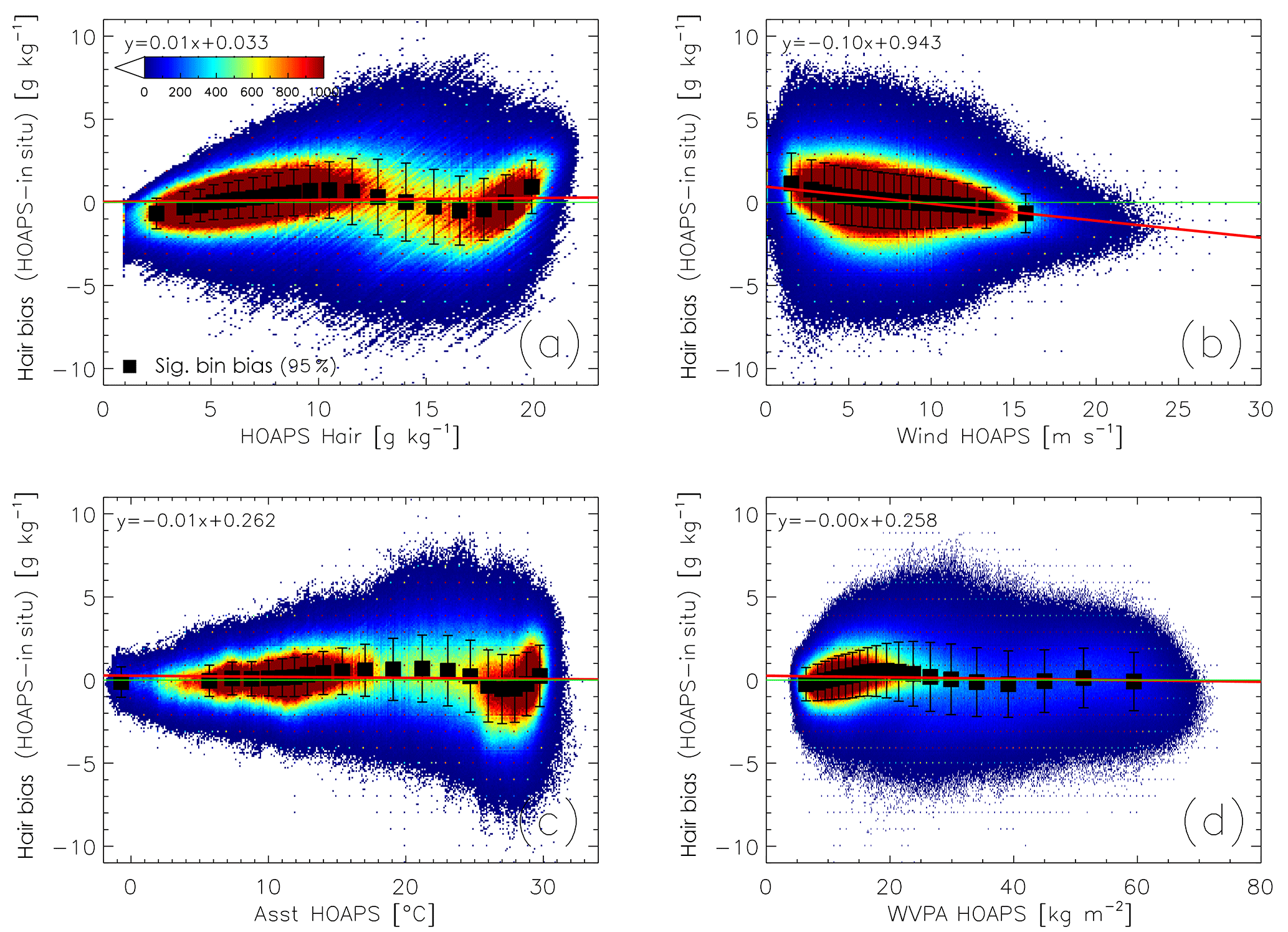
Figure 2Scatter density plots of qa bias (HOAPS 3.3 minus in situ, g kg−1) as a function of (a) qa (“Hair”), (b) U (“Wind”), (c) SST (“Asst”), and (d) vertically integrated water vapour (“WVPA”), based on global double collocations between 2001 and 2008. The black squares and error bars represent bin-averaged systematic uncertainties (significant at the 95 % level) and their SDs, whereby each bin contains 5 % of all double collocated matchups. Note that the bars include random uncertainty contributions from the satellite retrieval, the collocation procedure, and the in situ measurement uncertainty. Panel (a) is a revised version of Fig. 3 published in Kinzel et al. (2016).
Figure 1a presents the resulting collocation density for 2001–2008, exemplarily for qa. Matchups mainly occur in coastal regions (associated with buoys) and along major shipping lanes. By contrast, the Southern Ocean considerably lacks high-quality in situ measurements. The number of U and qs collocations exceeds those shown in Fig. 1a. For brevity, their distributions are not shown.
Figure 2a–d show exemplary scatter density plots of the qa bias (2001–2008) as a function of the atmospheric state parameters qa (“Hair”), U (“Wind”), SST (“Asst”), and vertically integrated water vapour (“WVPA”), resulting from the double collocation analyses. Overall, 13.8 million matchups contribute to each subplot. The illustrated bins are not equidistant; in fact, their width depends on the data density of the matchups. This implies that 5 % of all collocated pairs are assigned to a single bin. Analogously to Fig. 2, one-dimensional bias analyses are performed for both dU and dqs (not shown).
For qa values between 7 and 12 g kg−1, HOAPS 3.3 overestimates near-surface specific humidities (see Fig. 2a). Overestimations are also observed in the inner tropics, where qa is on the order of 20 g kg−1. In return, biases are negative for polar (<5 g kg−1) and subtropical (12–17 g kg−1) humidity regimes. The latter region is also subject to largest random uncertainties, which exceed 2 g kg−1. See Kinzel et al. (2016) and Prytherch et al. (2014) for more details on the analysis of HOAPS 3.3 qa and its resemblance to GSSTF 3 qa (Shie et al., 2012). The spatial distribution of these qa biases are shown in Fig. 1b. Specifically the underestimations (overestimations) over subtropical (tropical) oceans are well resolved. Humidity biases as a function of wind speed are illustrated in Fig. 2b. The distribution is somewhat linear, where low (high) wind regimes are overestimated (underestimated) in HOAPS 3.3. In contrast to the remaining atmospheric state parameters, the random uncertainty decreases fairly linearly with increasing wind speeds. The qa bias distribution as a function of SST (Fig. 2c) resembles that of the qa-dependent distribution (Fig. 2a) regarding regimes of over- and underestimation. A dependency of dqa on the total integrated water vapour (Fig. 2d) shows only few distinct features. Most matchups coincide with values below 20 kg m−2. With the exception of smallest values, these result in positive biases with respect to HOAPS 3.3. As the abscissa and ordinate variables in Fig. 2 are correlated, we investigated the contribution from artificial biases by illustrating dqa as a function of in situ qa, U, and SST. Results indicate that the percental difference of the mean bin values of HOAPS and DWD-ICOADS, range between 6 and 10 % (not shown). We are therefore confident that our approach is robust. However, we are aware of these pseudo-biases due to errors in the in situ records (e.g. Stoffelen, 1998), specifically in the tail regimes, which consequently leads to an increase of the HOAPS uncertainty estimates presented in Sect 4. Two-sided regression analyses could further reduce these spurious biases, which are envisaged for future HOAPS uncertainty characterizations.
A comparison of Fig. 2a and b indicates that the simple one-dimensional bias analyses may be misleading when it comes to HOAPS 3.3 qa-related uncertainty characterizations. Average qa off the Arabian Peninsula, for example, are on the order of 14–15 g kg−1 (not shown). According to Fig. 2a, this is associated with a HOAPS 3.3 qa underestimation, as is also seen in Fig. 1b. At the same time, climatological mean wind speeds are as low as 3–5 m s−1 (not shown), which goes along with a HOAPS 3.3 qa overestimation (Fig. 2b). This is no contradiction, but rather indicates that the HOAPS 3.3 qa retrieval seems to encounter challenges for specific humidity and wind regimes. Furthermore, a constraint to one-dimensional analyses implies for example that parts of the random uncertainties illustrated in Fig. 2a (bars) receive a systematic component in Fig. 2b (squares). This conclusion motivates to proceed with multi-dimensional bias analyses, where all possible atmospheric states, i.e. combinations of the four chosen atmospheric state parameters, are accounted for simultaneously. This approach finally allows for separating systematic from random uncertainties. Results illustrated in Fig. 2 can therefore be considered as a preliminary stage of the four-dimensional bias analyses introduced in Sect. 3.2, where each of the four atmospheric state variables (Fig. 2, x axes) represent one dimension.
3.2 Multi-dimensional bias analyses
The bulk formula for LHF is given by
where ρa is the density of moist air and LV the latent heat of vaporization. ρa is derived as a function of HOAPS 3.3 qa and near-surface air temperature. Likewise, LV is computed simultaneously as a function of HOAPS 3.3 SST. Assuming uncertainties in ρa and LV to be negligible and according to standard error propagation, the overall LHF uncertainty is a function of the systematic and random uncertainties introduced by the remaining parameters.
As to the dalton number CE, the estimates of Fairall et al. (2003) are applied by assigning 5 % (10 %) of systematic uncertainty of CE for wind speeds smaller (larger) than 10 m s−1. For wind speeds exceeding 20 m s−1, the estimate of Gleckler and Weare (1997) of 12 % is taken on. Independently of U, random uncertainties of 20 % are assigned, as proposed by Gleckler and Weare (1997).
In case of U, qs, and qa, the uncertainties are assumed to depend on the concurrent atmospheric state. The combination of qa, U, SST, and vertically integrated water vapour is thought to represent the concurrent atmospheric state best. Therefore, the one-dimensional consideration presented in Sect. 3.1 is expanded by creating four-dimensional look-up tables (LUTs) including 204 entries, respectively. The dimension is reflected in the exponent, whereas its base represents the number of bins per dimension. As described in Sect. 3.1, these bins are not equidistant. In case of dqa, bin means of each of the four dimensions are indicated by the x values of the black squares shown in Fig. 2a–d, respectively. The values of all four-dimensional vectors are essential for assigning instantaneous, absolute differences (HOAPS 3.3 minus in situ) to the correct LUT. By averaging the content of each bin, systematic and total random uncertainties finally result as a function of the four atmospheric state parameters. The approach is therefore geophysically motivated, but implemented in a statistical manner. Processing absolute measures of the observed differences allows for moving from a simple bias analysis to an uncertainty characterization. The resulting systematic uncertainties shown throughout Sect. 4 can therefore be treated as an upper boundary of a more simple bias distribution.
The multi-dimensional uncertainty characterization approach overcomes the issues introduced by data-sparse regions, such as the Southern Ocean and the tropical oceans (e.g. Kent and Berry, 2005). Here, it is knowingly turned away from the dependency on matchup density, which implies that the LUTs are valid on a global scale. Due to the immense data availability, their pairwise input biases are confined to matchups from 2001 to 2008 (dqa, dU) and from 1998 to 2001 and 2006 to 2008 (dqs). A thorough elucidation of the multi-dimensional bias analysis is presented in Kinzel et al. (2016), exemplarily for HOAPS 3.2 qa (Sect. 2c and Fig. 5a). Here, it is applied to all three bulk parameters, which results in both systematic and total random uncertainty LUTs.
3.3 Random uncertainty decomposition
The total random uncertainties introduced in Sect. 3.2 (and also those represented by the black error bars in Fig. 2) include random uncertainties associated with the collocation procedure (EC) and in situ measurement noise (Eins) (e.g. Bourras, 2006). To isolate the random retrieval uncertainty, , which is exclusively HOAPS related, MTC analysis is applied to matchups of U, qs, and qa for the time period 1995–2008. This section briefly summarizes the concept of random uncertainty decomposition. For more mathematical and technical details, the reader is referred to Kinzel et al. (2016).
MTC analysis includes a twofold TC (introduced by Stoffelen, 1998), whereupon double collocated data described in Sect. 3.1 serve as input. Triplets incorporating two independent in situ measurements and one HOAPS 3.3 pixel represent the first arrangement, whereas a single in situ record and two HOAPS 3.3 pixels of independent satellite instruments form the second triplet structure (see Fig. 1 in Kinzel et al., 2016). The collocation criteria applied in Sect. 3.1 are adopted and data poleward of 60∘ N–S are excluded to avoid biases associated with sea ice effects.
Subsequent to a bias correction with respect to the in situ measurements, the variances of differences between two independent data sources X and Y, that is VXY, are calculated following O'Carroll et al. (2008).
Given three data sources and two types of TCs, this results in six combinations of VXY. Next, error models for both ship and satellite records are defined (Kinzel et al., 2016). In case of ship records, these include Eins, whereas for satellite records they incorporate satellite sensor noise (EN, synthetically derived) and retrieval model uncertainty (EM). Applying these error models to the derived VXY, while explicitly accounting for error correlation terms, results in six equations incorporating Eins, EM, EN, and EC. These equations are successively solved for all random uncertainty sources as a function of U, qs, and qa, that is for 20 individual bins per parameter. Each of these bins include thousands of triple collocated matchups. Finally, is the required random satellite retrieval uncertainty, which is derived for all 20 bins as a function of U, qs, and qa.
MTC is a powerful tool to decompose total random uncertainties (i.e. ) inherent to LHF-related bulk parameters in order to isolate the random retrieval contribution . Depending on the magnitude of the respective bulk parameter, the fractional contribution from to Esum is finally derived. That is, each entry of the total random uncertainty LUTs introduced in Sect. 3.2 is “adjusted”.
Section 4.1 presents a statistical summary of the instantaneous, decomposed random uncertainties inherent to U, qs, and qa.
3.4 Deriving HOAPS 3.3 LHF-related uncertainties
The uncertainties in LHF are caused by uncertainties in all bulk input parameters contributing to Eq. (1). Assuming the underlying parameterizations to be correct, LHF uncertainties can thus be derived by carrying out standard error propagation. These uncertainty estimates are assigned to each HOAPS pixel, depending on the four atmospheric state parameters.
Total instantaneous LHF uncertainties, σLHF, are derived as follows:
where x and y are placeholders of U, qs, qa, and CE. rxy is the correlation coefficient between x and y. For each combination of x and y, the average of daily global mean correlation coefficients between 1995 and 2008 is applied. Global mean coefficients are preferential compared to instantaneous rxy for two reasons. First, the amount of instantaneous data for a specific region is limited, which may distort the results of the correlation analysis. Second, omitting all correlation-related terms in Eq. (2) modifies σLHF,sys by merely 0.5±5 W m−2 (not shown), which indicates that these terms do not receive much weight after all.
σx and σy are total uncertainties in x and y. These can be decomposed into systematic and random components. Note that the random component has been corrected for collocation and in situ uncertainty effects (see Sect. 3.3) and already represents the random retrieval uncertainty .
N is the number of HOAPS 3.3 satellite observations (N=1 for instantaneous LHF uncertainties). In case of temporal and spatial averaging over a sufficiently long time period, the random component becomes negligibly small. Sampling uncertainties do not exist on an instantaneous basis and are therefore not considered in Eqs. (2)–(3).
3.5 Sampling uncertainty
In addition to systematic and random uncertainties, inhomogeneous sampling may occur, specifically when temporal resolution in observations are coarse. As remotely sensed data are measured at selected times only, temporal sampling uncertainties therefore become an issue (Gulev et al., 2010), as the diurnal cycle may not be captured correctly.
Daily mean sampling uncertainties of HOAPS 3.3 LHF-related parameters are derived, using high-resolution buoy measurements. Overall, data of eight tropical (PMEL, hourly resolution) and 15 extratropical (NDBC, 10 min resolution) moored buoys account for a possible climate regime dependency. All chosen buoy records comprise several years of data (1995–2008) and hardly show temporal data gaps. Here, the approach by Tomita and Kubota (2011) is followed to derive the sampling uncertainties by simulating two satellite data overpasses per day, using the buoy values. In case of U and SST, records are corrected for sensor heights and cool skin effects, respectively, as explained in Sect. 2.2. In situ LHF are computed by means of the COARE 2.6a algorithm (Fairall et al., 2003). Daily means of “true” buoy data are derived by averaging all daily buoy records, where only high-quality data (indicated by quality flags 1–2) are considered. The weighted average of the two closest (in time) “true” buoy observations to local satellite overpasses corresponds to the so-called “simulated” satellite data record (Tomita and Kubota, 2011, their Fig. 2). All daily sampling uncertainties are derived as a function of the number of simultaneously operating SSM/I instruments. These daily values form the basis for the monthly averages of selected parameters (Esmp), which are outlined in Table 2 (Sect. 4.4). The estimates are global means; an earlier, regime-dependent investigation resulted in negligible differences. This implies that monthly mean systematic uncertainties do not exhibit a latitudinal dependency.
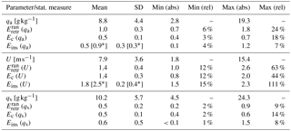
Table 1Absolute and relative random statistical measures resulting from the multi-dimensional LUTs, i.e. MTC and random uncertainty decomposition (Sects. 3.2 and 3.3). “SD” is standard deviation, “abs” is absolute, and “rel” is relative. Apart from the LHF-related bulk parameters themselves (U, qs, and qa), global mean ranges of the random retrieval (), random collocation (Ec), and random in situ measurement uncertainty (Eins) are shown. Relative measures result from bin-wise relative uncertainty calculations. For comparison, the asterisks indicate respective estimates published in Kent and Berry (2005), which are based on a semivariogram approach.
4.1 Magnitudes of HOAPS 3.3 decomposed random uncertainties
Table 1 presents a statistical summary of the instantaneous random uncertainty decomposition for the bulk parameters U, qs, and qa, following the approaches described in Sects. 3.1 to 3.3. Note that EN is not included, as its synthetically derived value remains constant throughout the respective parameter range (for procedure, see Kinzel et al., 2016). Asterisked values indicate global mean weighted averages and pooled variances of Kent and Berry (2005), resulting from a semivariogram approach. These are based on their Fig. 1, taking the illustrated grid averaged random uncertainties, the SD, and the number of observations into account. In the following, individual contributions to the overall random uncertainties are discussed but not shown in terms of supplementary figures.
(qa) ranges between 0.7 and 1.8 g kg−1, where minima (maxima) are found below 5 g kg−1 (between 13 and 17 g kg−1) qa regimes. Whereas largest relative uncertainties are associated with polar qa values (3–5 g kg−1), lowest relative contributions below 10 % are confined to the inner tropics (20 g kg−1). On average, both Ec (qa) and Eins (qa) are approximately half the size of (qa). The average of Eins (qa) is 0.4 g kg−1 below the mean estimate of Kent and Berry (2005). It is hypothesized that the lower estimate of Eins (qa) is a direct consequence of the rigorous in situ filtering procedure prior to MTC analysis. The difference may furthermore be triggered by the fact that Kent and Berry (2005) include data records dating back to the 1970s and 1980s, which may imply that ship records are included which do not fulfill the here-applied quality control standards. In contrast to (qa), Eins (qa) increases rather linearly with qa, which implies that smallest (largest) random in situ measurement uncertainties are found for lowest (highest) qa. In contrast, Ec (qa) shows a similar distribution as (qa), yet with considerably smaller amplitude. These random collocation uncertainties range between 0.4 and 0.7 g kg−1, corresponding to 3–18 %. A graphical illustration of the qa random uncertainty decomposition is shown in Kinzel et al. (2016) (their Fig. 2).
In case of U, all random uncertainties tend to be larger compared to qa in a relative sense. In contrast to qa, all three relative uncertainties exhibit a clear increase over large ranges of U, where minima and maxima in (U) (Eins (U), Ec (U)) range between 1.0 and 2.6 m s−1 (1.5–2.3 m s−1, 0.8–2.0 m s−1). Whereas (U) and Eins (U) are fairly constant for moderate wind speeds before continuously increasing, Ec (U) seems to already saturate for mean wind speeds on the order of 10 m s−1 (not shown). Similar to Eins (qa), the Eins (U) estimate of Kent and Berry (2005) is roughly 40 % larger. Again, this difference is suspected to arise from the differences in the data set compositions. Kent and Berry (2005) furthermore elucidate that no corrections for height or adjustments to the Beaufort scale have been applied to their data, which would have caused a reduction in random uncertainty of 13±1 %, according to the authors. However, Eins (U) almost exclusively represents the largest contribution to the random uncertainty budget of U. For all random uncertainty sources, strong wind regimes are linked to smallest relative uncertainties on the order of 12–15 %. In low-wind regimes, however, relative uncertainties exceed 50 % to even 100 %.
Both absolute and relative contributions from qs-related random uncertainties remain well below those of qa. Global mean values of all three random uncertainty sources are on the order of 0.5–0.6 g kg−1. Regarding (qs), this is comparable to the value published in e.g. McClain (1989), who estimated the global RMSE of AVHRR-derived SST to be on the order of 0.6–0.7 K ( 0.4–0.5 g kg−1). Similar to (U), (qs) (Eins (qs)) shows a positive proportionality with largest values of 0.9 g kg−1 (1.5 g kg−1). As for Eins (U), Eins (qs) exceeds (qs), specifically for qs larger than 8 g kg−1. In contrast to qa, relative uncertainties are smallest in extratropical regimes with contributions of merely few percent. Largest relative uncertainties remain well below those of qa and are on the order of 8–14 %.
4.2 Global patterns of HOAPS 3.3 random retrieval uncertainties
The results presented in Sect. 4.1 are expanded by showing the global patterns of in two-dimensional space.
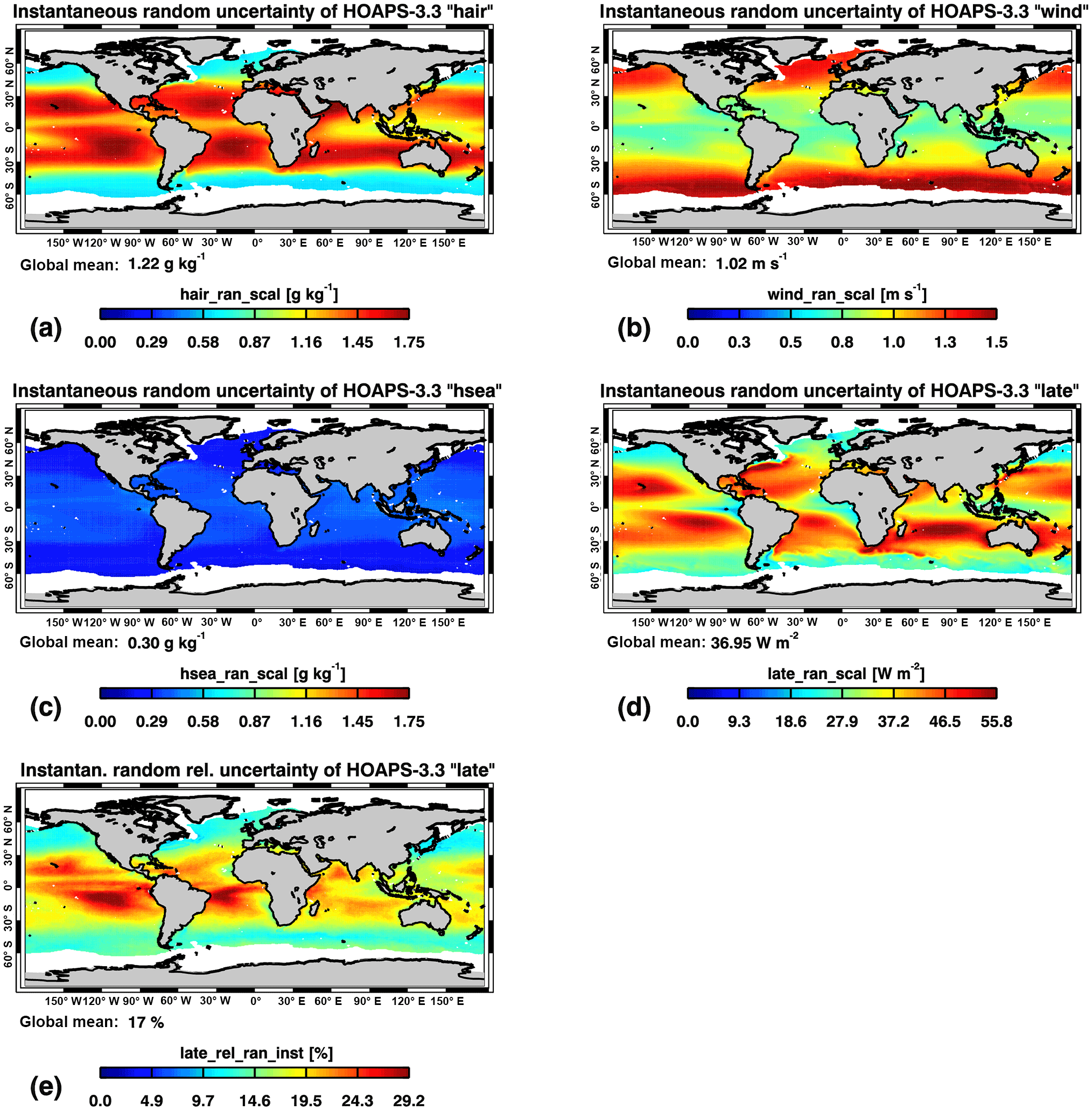
Figure 3Temporal averages (1988–2012) of HOAPS 3.3 instantaneous of (a) qa (“hair”), (b) U (“wind”), (c) qs (“hsea”), and (d) LHF (“late”). (e) Relative random retrieval uncertainty of HOAPS 3.3 LHF with respect to its natural variability. This variability is defined as the range between the 5th and 95th percentile of instantaneous LHF between 2000 and 2008. The global averages (text strings) were derived by considering a latitudinal cosine dependency. All patterns result from the multi-dimensional bias analyses, MTC, random uncertainty decompositions, and, in case of panel (d), uncertainty propagation described in Sects. 3.2–3.4. Note that the colour bar ranges of panels (a) and (c) are identical to allow for direct comparisons.
Depending on the time period and thus on the number of SSM/I and SSMIS instruments in operation, the monthly global mean sum of instantaneous observations per grid cell ranges from approximately 90 (1988) to 650 (2006). As a consequence, monthly means of are considerably below the systematic counterpart (see scaling effect of N in Eq. 3). Specifically from 1991 onwards, monthly globally averaged of LHF-related parameters only reach 0.5–3 %. This reduction becomes even more striking when investigating multi-annual or even climatological means; LHF-related virtually vanishes on these scales. An increase (decrease) in these climatological random uncertainty values often directly results from a decrease (increase) in the number of pixel-level observations and thus not from a physical change due to shifts in the climate. This implies that results of trend analyses in random uncertainties, for example, may be misinterpreted. Therefore, the attention is drawn to the pixel-level (instantaneous) random uncertainty fields. This instantaneous point of view causes their orders of magnitude to be similar to the results of presented in Table 1. Note that the global averages shown in Fig. 3 in the form of text strings are cosine-weighted, whereas the means illustrated in Table 1 do not take a regional dependency into account.
Figure 3 shows the instantaneous patterns of HOAPS 3.3 LHF-related parameters between 1988 and 2012. The magnitudes presented in Fig. 3a are below those shown in Fig. 2a, as the random uncertainties have been corrected for the impact of Eins (qa) and Ec (qa) (Sect. 3.3). Maxima above 1.5 g kg−1 are located over all subtropical ocean basins, where qa is on the order of 13–17 g kg−1. A reduction within the inner tropics is clearly resolved, specifically over the warm pool region. (qa) sharply decreases poleward to values of 0.6–0.9 g kg−1. The global mean instantaneous (qa) takes on a value of 1.2 g kg−1.
The distribution of instantaneous (U) (Fig. 3b) shows a rather reversed pattern of qa and closely resembles the climatological distribution of U itself. The global mean is given by 1.0 m s−1. Global maxima cover large areas of the extratropical oceans, specifically over the Southern Ocean. Here, averages partly exceed 1.5 m s−1. However, this results in less than 15 % retrieval uncertainty in a relative sense (not shown). In contrast, instantaneous (U) remain low (that is, below 0.8 m s−1) over the (sub-)tropical ocean basins. This also applies to the warm pool area, which indicates a maximum in relative contribution close to 20 % due to climatological low wind speeds (not shown).
The pattern of instantaneous (qs) (Fig. 3c) resembles that of qa. However, the global mean magnitude of 0.3 g kg−1 represents only 25 % of the atmospheric counterpart. Absolute maxima on the order of 0.4 g kg−1 are located over the Indo-Pacific warm pool region, which stands in contrast to the local (qa) minimum in that region. The comparatively small (qs) also find expression in the low global mean relative uncertainty of 2 % (not shown). Values exceeding 4 % are confined to the extratropical ocean basins in both hemispheres.
Instantaneous (LHF) (Fig. 3d) shows a strong proportionality to the climatological mean LHF pattern. In that respect, maxima are generally located over the subtropical central parts of all ocean basins (specifically the Indian Ocean) as well as along the western boundary currents (WBCs). In these areas, values are found in excess of 50 W m−2. Apart from extratropical minima, low values in the tropics are confined to the eastern margins of the basins and the warm pool region.
Figure 3e shows the instantaneous random uncertainty of LHF relative to its natural variability. For each grid box, this variability is derived as the difference between the 5th and 95th percentile of instantaneous LHF observations between 2000 and 2008 (F13 platform only). Globally averaged, the relative random uncertainty equals to 17 %. Due to the large range of LHF along the WBCs and over the central Indian Ocean, the absolute maxima seen in Fig. 3d are not resolved in Fig. 3e. Largest relative uncertainties exceeding 25 % are confined to the southern central tropical Pacific and along the equatorial Atlantic.
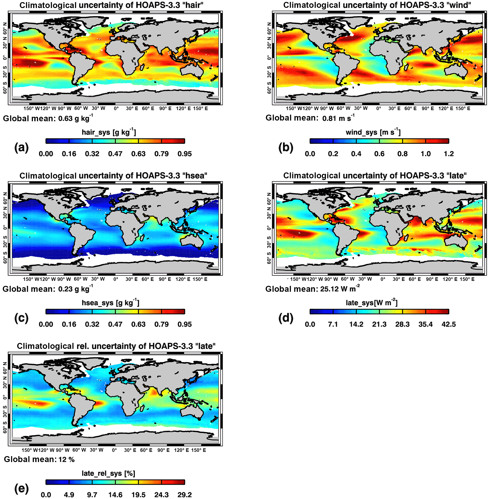
Figure 4HOAPS 3.3 climatological total uncertainties (Eclim) of (a) qa (“hair”), (b) U (“wind”), (c) qs (“hsea”), and (d) LHF (“late”). Eclim is defined as the mean root-mean-squared sum of Esys, , and Esmp (1988–2012). (e) Climatological mean relative Eclim (LHF) with respect to its natural variability. This variability is defined as the range between the 5th and 95th percentile of instantaneous LHF between 2000 and 2008. The global averages (text strings) were derived by considering a latitudinal cosine dependency. All patterns result from the multi-dimensional bias analyses and subsequent uncertainty propagations described in Sects. 3.2 and 3.4. Note that the colour bar ranges of panels (a) and (c) are identical to allow for direct comparisons.
4.3 Global patterns of HOAPS 3.3 climatological uncertainties
Figure 4 shows the distribution of the climatological uncertainties (Eclim) for LHF and its related bulk parameters. Eclim is defined grid point wise as the mean root-mean-squared sum of instantaneous Esys, , and Esmp between 1988 and 2012. As the contribution from and Esmp converges towards 0 % due to the vast number of observations, Fig. 4a–e can also be treated as the systematic uncertainty distribution.
In an absolute sense, Fig. 4a mirrors the bias distribution shown in Fig. 2a. Eclim (qa) (Fig. 4a) generally range between 0.4 and 0.9 g kg−1, where the global mean of 0.63 g kg−1 is approximately half the size of the instantaneous random counterpart shown in Fig. 3a. Maxima are found over the tropical central and western Pacific Ocean as well as the Caribbean and off the easternmost tip of South America. In the framework of a LHF intercomparison study, Smith et al. (2011) argue that satellite products have difficulties estimating qa due to persistent stratus clouds, as observed west of Peru over the tropical eastern Pacific. This conclusion may be the cause for the elevated systematic uncertainties over the tropical eastern Pacific. In contrast, minima are located along both extratropical belts poleward of 50–60∘ N–S. Isolated minima also lie over the subtropical eastern margins of all ocean basins in the vicinity of 15–30∘ N–S, specifically over the Pacific basin. Interestingly, regions of comparatively low systematic uncertainties often coincide with regional maxima in random uncertainties (compare Fig. 3a). According to Fig. 2a, biases are smallest for climatological mean qa of 4–5 and 13 g kg−1, which fits well to the mentioned minima in Fig. 4a. Likewise, absolute bias maxima for qa of 10 and 16–17 g kg−1 are resolved in both Figs. 2a and 4a.
The global mean of Eclim (U) shown in Fig. 4b equals to 0.81 m s−1. On the one hand, maxima exceeding 1 m s−1 are located along the extratropical storm tracks, specifically over the Northern Hemisphere. On the other hand, local maxima are found along broad regions at 30∘ S and further equatorward over the central Indian Ocean, off the Arabian Peninsula (both monsoon-related), and the central northern tropical Pacific. With the exception of the Southern Ocean, this is in line with Brunke et al. (2011), who conclude that reanalysis, satellite, and combined data sets tend to overestimate wind speeds compared to in situ records of inertial dissipation wind stresses, specifically over strong wind regimes. Monsoon-related characteristic features of Indian Ocean LHF variability, which also exhibit an impact on climatological uncertainties, are elucidated in e.g. Mohanty et al. (1996). Minima on the order of 0.5 m s−1 are mostly confined to the eastern margins of all ocean basins (Fig. 4b). The maxima over the northern hemispheric storm track are associated with climatological mean wind speeds of 9–11 m s−1. This range also reveals largest positive biases in the one-dimensional bias consideration with respect to the in situ source (analogously to Fig. 2, but not shown for U). This also targets the maximum over the central northern tropical Pacific and all southern hemispheric maxima along 40–50∘ S. Although climatological mean wind speeds maximize over the Southern Ocean, respective systematic uncertainties rather show a slight poleward decrease. Again, this is in line with results from the one-dimensional dU analysis (not shown), which indicates that systematic uncertainties reduce for wind speeds above 12 m s−1. Likewise, absolute bias minima are associated with low-wind regimes on the order of 4–6 m s−1. Climatologically lowest wind speeds of 2–4 m s−1 are for example found along the Pacific coast of Central America (15∘ N), over the Arabian Sea, and over the Indo-Pacific warm pool region. HOAPS 3.3 tends to underestimate these wind speeds, as is mirrored in moderate Eclim (U) (Fig. 4b).
The climatological uncertainty estimates illustrated in Fig. 4b exceed those found in e.g. scatterometer records in comparison to buoy measurements (e.g. Verhoef et al., 2017). On the one hand, this is linked to the fact that estimates in Fig. 4b should be treated as upper boundary uncertainty estimates. On the other hand, scatterometers are specifically designed to derive near-surface wind speeds at highest accuracy. Passive microwave measurements, in return, allow for a much broader range of applications, which is a unique feature of HOAPS. An inclusion of scatterometer data into the HOAPS wind speed retrieval was not envisaged, due to differing overflight times and data coverage, that is additional uncertainties of unknown magnitude. Further potential uncertainty sources, which may contribute to the distribution shown in Fig. 4b, target currents, sea states, and the treatment of air mass density (i.e. the concept of stress-equivalent wind speeds; e.g. de Kloe et al., 2017).
Eclim (qs) covers the range of 0.1–0.6 g kg−1 and its global average is given by 0.23 g kg−1 (Fig. 4c). The pattern reflects a latitudinal dependency, which is equivalent to smallest (largest) biases towards the poles ((sub-)tropics). This observation is not generally valid, as is shown by the comparatively low values over large parts of the eastern tropical Pacific and Atlantic. Distinct maxima are found over the Arabian Sea and along northwestern Australia, the Caribbean, and west of Madagascar. Narrow bands of elevated systematic uncertainty are also resolved along the WBCs. With the exception of the WBCs, the regions of maxima are exposed to qs in the range of 20–22 g kg−1.
Figure 4d shows the resulting Eclim (LHF). It closely resembles that of the global mean LHF pattern itself with values ranging between roughly 15 and 50 W m−2 and a global mean of 25 W m−2. Relating this pattern to Fig. 4a–c shows a substantial contribution of Eclim (qa) to the absolute maximum of Eclim (LHF) in the northern–southern tropical central Pacific, the Caribbean, and the western tropical South Atlantic (compare Fig. 4a). However, due to the large climatological mean LHF, respective relative systematic uncertainties of qa are merely on the order of 5–7 %. Correspondingly, imprints of Eclim (U) are clearly seen along the WBCs, the central Indian Ocean (10–15 % in a relative sense), and off the Arabian Peninsula (partly exceeding 15 %) (Fig. 4b). Likewise, the maxima in Eclim (LHF) over the Arabian Sea, along the northwestern coast of Australia, and close to Madagascar show the footprint of Eclim (qs) (Fig. 4c). However, relative systematic uncertainties in qs generally do not exceed 2.5 %. Locally, isolated Eclim (LHF) maxima are resolved along 35∘ S. Specifically over the Agulhas Current, Santorelli et al. (2011) conclude that different satellite data sets show discrepancies, as they are not able to properly handle strong LHF associated with storm systems and potential LHF amplifications due to dry air advection northwards from the Antarctic (Grodsky et al., 2009). Furthermore, note that the maximum in the Arabian Sea is somewhat special, in as much as climatological mean LHF in this region are elevated, yet not extraordinarily large. This striking uncertainty maximum may be linked to occasionally occurring advection of hot, dry air masses from the deserts, which poses problems to the HOAPS 3.3 satellite retrieval. This hypothesis is strengthened by the fact that Iwasaki et al. (2014) show largest deviations in HOAPS 3 qs with respect to their reference climatology, which are not seen in the remaining data sets.
Figure 4e relates Eclim (LHF) to its natural variability (compare Sect. 4.2). The global average is on the order of 12 %. Apart from the WBC regimes and the Southern Ocean, largest relative uncertainties are in line with the Eclim (LHF) maxima illustrated in Fig. 4d.
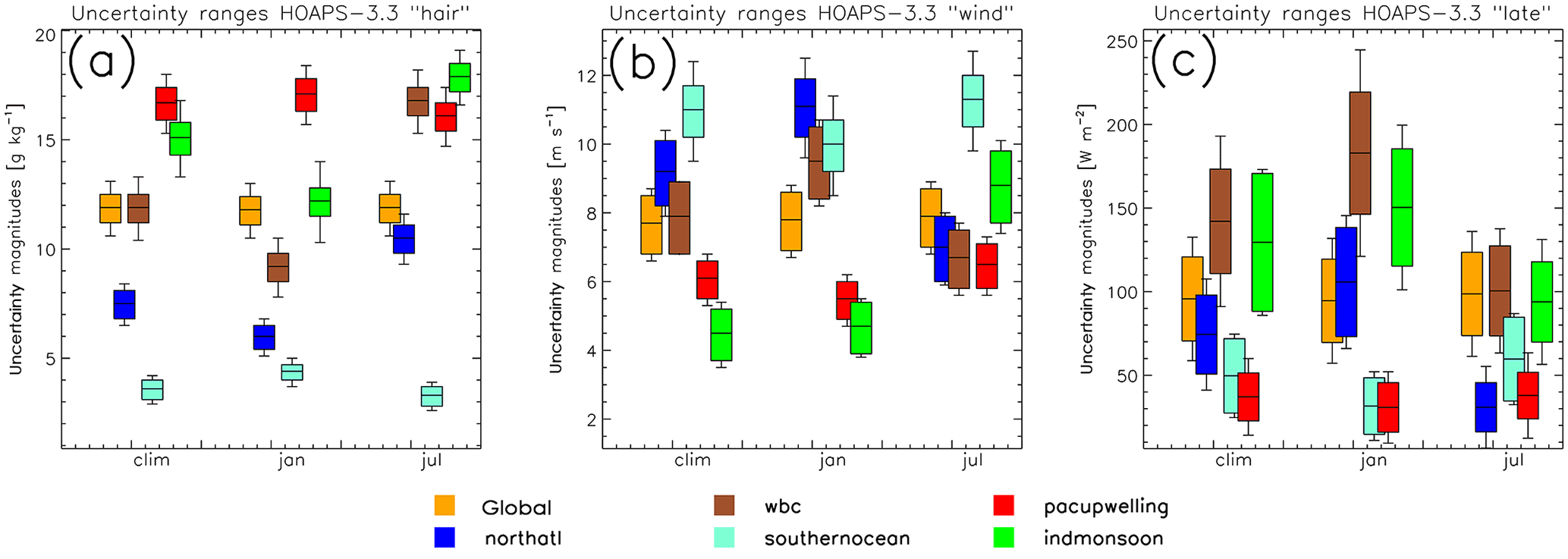
Figure 5(a) Expected ranges of qa (“hair”) as a function of different regions and seasons. The colour-coded boxes show Eclim (1988–2012), whereas the bars indicate the average instantaneous random uncertainty component (1988–2012). The following regions are presented: global (orange), North Atlantic (60∘ W–5∘ E, 35–65∘ N; dark blue), North Atlantic western boundary current (WBC, 60–80∘ W, 30–40∘ N; brown), Southern Ocean (50–60∘ S; cyan), Pacific upwelling regime (80–100∘ W, 5∘ N–5∘ S; red), and Indian monsoon region (50–75∘ E, 15–30∘ N; green). (b) As for panel (a), but for U (“wind”). (c) As for panel (a), but for LHF (“late”).
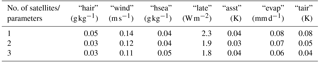
Table 2Average of monthly mean HOAPS 3.3 LHF-related sampling uncertainties (Esmp) as a function of simultaneously operating SSM/I instruments (1995–2008). qa is “hair”, U is “wind”, qs is “hsea”, LHF is “late”, SST is “asst”, E is “evap”, and air temperature is “tair”. All magnitudes are negligible compared to the instantaneous random () and climatological uncertainties (Eclim) presented in Sects. 4.2 and 4.3.
4.4 Monthly mean HOAPS 3.3 sampling uncertainties
Table 2 summarizes the average of monthly mean sampling uncertainties of several LHF-related HOAPS 3.3 parameters as a function of concurrently operating SSM/I instruments. From a climatological perspective, all magnitudes are negligibly small compared to respective systematic uncertainties. SST-related parameters show largest sampling uncertainties when three SSM/I instruments are simultaneously operating. This is not contradictory, as HOAPS 3.3 SST are AVHRR-based and thus not linked to the coverage of SSM/I instruments. Regarding the main bulk parameters, orders of magnitude closely resemble those of monthly mean scaled (not shown). It is concluded that their relative contribution to the monthly mean uncertainty budget is on the order of merely 1–2 %. However, one should keep in mind that sampling uncertainties become essential on considerably shorter timescales, i.e. in the framework of daily analyses.
4.5 Fractional contributions to total HOAPS 3.3 LHF uncertainty
Simply comparing Fig. 4a–c to d allows for qualitatively assessing which LHF-related parameter contributes most to Eclim (LHF). However, this does not permit a quantitative conclusion. Following a modified version of the “Q-term” approach demonstrated in Bourras (2006), Eclim (LHF) is decomposed into fractions associated with U, qs, qa, and CE. Results indicate that the global mean contribution from Eclim (qa) is largest (60 %). This specifically targets the central northern and southern tropical Pacific, the Caribbean, the regime off the eastern tip of South America, and the central Indian Ocean. This finding is in line with that of Iwasaki et al. (2014), who show that HOAPS 3 qa contributes most to the observed deviation in E with respect to their reference climatology.
On average, the contribution from Eclim (U) takes on a value of 25 %. Local hotspots are considerably larger, especially over the Arabian Sea, along the WBCs, and off Northwestern Australia. The fractional contributions due to both Eclim (qs) and Eclim (CE) equal to 7.5 %, respectively. Eclim (qs) is largest over the Arabian Sea (SST retrieval issues due to dust particles), whereas Eclim (CE) maximizes over the central Indian Ocean and along the North Atlantic WBC. The latter has also been shown by Bourassa et al. (2013), in as much as accuracy issues in CE tend to occur over very low and very high wind speed regimes.
All findings are in line with Bourras (2006), Liu and Curry (2006), Grodsky et al. (2009), and Santorelli et al. (2011), who conclude that the main LHF uncertainty sources are related to the accuracy of qa (and U). Similar conclusions are drawn by e.g. Tomita and Kubota (2006), who show that the main source of discrepancy between tropical satellite and buoy estimates may be attributed to the accuracy of qa. The findings of the above-quoted studies are restricted to either regional analyses, considerably shorter investigation periods, and/or comparatively thin reference databases. Again, this points at the high value of the presented HOAPS 3.3 uncertainty analyses.
4.6 Regional and seasonal HOAPS 3.3 uncertainty analyses
Global mean and Eclim of LHF-related HOAPS 3.3 parameters are fairly constant in time throughout the whole climatology (Figs. 3 and 4). Absolute deviations from the global mean LHF (qa, U) uncertainty become as large as 18 % (3, 8 %). Apart from seasonal signals, these are footprints of distinct local anomalies. On the one hand, these anomalies seem to originate from events that temporarily modify the global climate. On the other hand, Figs. 3 and 4 resolve considerable regional variability. Therefore, the aim is to (1) identify climate features that are manifested in both temporal and spatial uncertainty anomalies and discuss their origin (descriptive only). At the same time, (2) regional uncertainty differences shall be highlighted by focusing on climate hotspots (Fig. 5a–c).
(1) The imprints of moderate to strong El Niño events during boreal spring 1998 and 2010 are manifested in LHF-related Eclim and . During these events, wind speeds over the Pacific upwelling regime are 1.5–2.0 m s−1 below the climatological average. As has been mentioned in Kinzel et al. (2016), this causes an increase in systematic uncertainties in U. Along with an enhanced Eclim (qs), the respective Eclim (LHF) over the Pacific upwelling regime reaches 25 W m−2, specifically during boreal spring 1998. This is approximately 10 W m−2 above the seasonal mean and more than 50 % of climatological mean LHF. As qa are anomalously high with 20 g kg−1, (qa) is up to 0.2 g kg−1 below the seasonal mean (see Fig. 2 in Kinzel et al., 2016, for clarification).
By contrast, global minima in Eclim (LHF) and (LHF) are confined to boreal autumn 1991, taking on a mean value of 20 and 33 W m−2, respectively. These estimates are 20 and 11 % below their climatological averages and are associated with absolute minima in HOAPS 3.3 LHF. The comparatively small systematic component is induced by Eclim (U) (Eclim (qs)) of −8 % (−14 %). The absolute minimum in LHF and its uncertainties during 1991 is a footprint of the Mount Pinatubo eruption, which caused low-biased SST due to AVHRR aerosol issues and thus unrealistically low near-surface humidity gradients (Romanova et al., 2010). Amongst others, this shortcoming in the HOAPS 3.3 climatology has already been picked up by Andersson et al. (2011).
(2) Figure 5a–c summarize the ranges of seasonal, regime-dependent uncertainty distributions. The colour-coded boxes in Fig. 5a–c represent the expected parameter ranges when considering multi-annual (1988–2012) means of systematic uncertainty contributions, that is Eclim. At the same time, the error bars indicate the instantaneous random uncertainty components, that is . Both are shown separately, as they are independent of each other. With few exceptions, the random uncertainty contributions exceed the systematic counterpart, as is also mirrored in Figs. 3 and 4.
Figure 5a indicates that the total uncertainty ranges in qa are largest in (sub-)tropical regimes, concurrent to high qa. In contrast to the Pacific upwelling region (red) and the Southern Ocean (cyan), the seasonal qa variability over the Indian monsoon regime (green), the North Atlantic basin (dark blue), and specifically the North Atlantic WBC (brown) is striking. This also finds expression in differences in absolute uncertainties of up to ±0.6 g kg−1 between January and July. Largest uncertainties are on the order of ±2.40 g kg−1 and are confined to the Indian summer monsoon season, whereas smallest uncertainties around ±1 g kg−1 occur over the Southern Ocean.
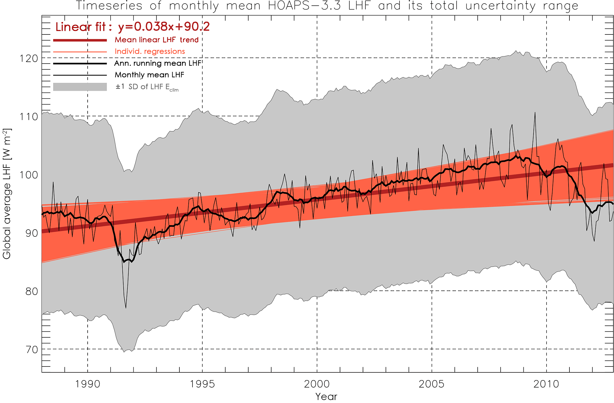
Figure 6The thin (thick) black line shows the monthly (annual running mean) time series of HOAPS 3.3 LHF (70∘ S–70∘ N, cosine-weighted average). The dark red line illustrates the linear trend, which takes on a value of 4.5 W m−2 per decade (p<0.00001, based on a two-tailed t test). The grey shading represents ±1 SD of the annual running mean Eclim (global average). The light red regression lines were iteratively derived following Kelly (2007) by taking ±1 SD of Eclim into account.
Climatological regional wind speeds range between 4.5 and 11 m s−1 (Fig. 5b). As for qa, the seasonality is most pronounced over the Indian monsoon region, WBC, and the North Atlantic. Largest total uncertainties exceeding ±2 m s−1 throughout the year are observed over the Southern Ocean, which is primarily due to large (U) (compare Fig. 3b). The Indian monsoon region is somewhat special, in as much as summertime total uncertainties are largest on a global scale, while wintertime ranges are almost 50 % lower.
Figure 5c presents regionally dependent LHF and associated uncertainty ranges. As for Fig. 5a and b, seasonality is most distinct over the North Atlantic, WBC, and the Indian monsoon region. Largest Eclim (LHF) exceeding ±35 W m−2 are confined to the WBC regime (specifically during winter) and the monsoon region (climatological average, compare also Fig. 4d). Total uncertainty ranges maximize along the WBC, where ±65–95 W m−2 are to be expected, which is 2–3 times larger compared to the ranges observed along the Pacific upwelling regime. Grodsky et al. (2009), for example, recall that an accurate representation of LHF along the Gulf Stream is challenging due to strong surface currents and SST gradients as well as intraseasonal dependencies of how the stratified atmospheric boundary layer amplifies air–sea interactions. This reasoning may also apply to the Agulhas and Kuroshio region. The wintertime WBC uncertainty maximum is particularly caused by vast (LHF) of up to ±60 W m−2 (see also signal in Fig. 3d). By contrast, regional Eclim (LHF) become largest in the Indian monsoon region, where their climatological average is on the order of ±40 W m−2 (compare also Fig. 4d).
4.7 Uncertainty application: trends in HOAPS 3.3 LHF
Figure 6 shows the HOAPS 3.3 global monthly mean LHF (thin black line) between 1988 and 2012 (70∘ S–70∘ N, cosine-weighted average). The global minimum below 80 W m−2 during boreal summer 1991 is linked to the Mount Pinatubo eruption. Overall maxima on the order of 110 W m−2 occur during 2008 and 2009.
The bold black line in Fig. 6 shows the annual running mean climatology of HOAPS 3.3 LHF. On average, it increases by roughly 4.5 W m−2 (4.7 %) per decade (dark red line). If uncertainty ranges were discarded, this trend would be considered as significant at the 95 % level (p<0.00001, based on a two-tailed t test). The addressed uncertainty estimates are illustrated as grey shadings and represent ±1 SD of the 12-month running mean Eclim (global average). They take on a mean value of ±17 W m−2. A Bayesian approach to linear regression is applied including LHF uncertainty estimates following Kelly (2007), which yields a large range of linear trends (light red lines). Although the majority has a positive slope, some even indicate a climatological decrease in LHF. In light of the illustrated uncertainty range, the mean upward trend in HOAPS 3.3 LHF (dark red line) should therefore be treated with caution, as the magnitude of linear increase lies well within the grey shaded area.
The overall increase in LHF has been elucidated in several studies concerning various LHF data sets (e.g. Liu and Curry, 2006; Yu and Weller, 2007; Santorelli et al., 2011; Yu et al., 2011; Iwasaki et al., 2014). The authors attribute it to increases in both qs (i.e. SST) and U, whereas the latter may be linked to stronger Hadley and Walker circulations (Cess and Udelhofen, 2003). The global mean increase of 9 W m−2 between 1981 and 2002, as is seen in Objectively Analyzed Air–Sea Heat Fluxes (OAFlux; Yu and Weller, 2007), is on the order of 10 %, which is in line with findings of Santorelli et al. (2011) and those illustrated in Fig. 6 of the present work.
Figure 6 also shows that recent global means decrease again. Time series analyses for single satellite instruments suggest that this is a physical signal (i.e. associated with either multi-annual variability or a climate signal) rather than being associated with intercalibration issues among SSM/I and SSMIS instruments. Additionally, the decrease may also be attributed to the slight negative SST bias from 2011 onwards. This bias is caused by anomalously high NOAA-19 sensor noises, which themselves may be traced back to erroneous flag assignments during cloud detection. This is thought to cause up to 5–10 % reduction in LHF. Closer investigations that involve other LHF climatologies exceed the scope of this study but are needed to interpret this gradual decay.
First intercomparisons of HOAPS 3.3 LHF to in situ and further satellite climatologies have been carried out, where preliminary results indicate that nearly all compared data sets lie within the uncertainty range presented in Fig. 6 (not shown). A more detailed intercomparison study is envisaged; it will benefit from uncertainty estimates available in NOCSv2.0 and allow for concluding whether global mean deviations among the data sets lie within or outside of the HOAPS 3.3 prescribed uncertainty range.
By means of multi-dimensional bias and MTC analyses, a universal approach for characterizing systematic, random retrieval, and sampling uncertainties inherent to HOAPS 3.3 LHF-related parameters has been presented. The multi-dimensional approach overcomes the issues of sparse data densities in remote regions, as it expresses the uncertainties as a function of the ambient atmospheric conditions. At the same time, MTC enables a decomposition of random uncertainty sources to isolate the contribution from the satellite retrieval. Both methods represent the main procedures to arrive at pixel-level uncertainty information, which essentially increases the value of HOAPS 3.3. As to sampling uncertainties, monthly mean estimates have been calculated following the approach of Tomita and Kubota (2011). To conclude, HOAPS 3.3 can be considered as the first LHF satellite-only climatology including instantaneous and gridded uncertainty estimates. As the method can be easily transferred to other retrievals, it lays the foundation for uncertainty characterizations of further LHF-related data sets, which increases the significance of this work.
It has been shown that maxima of systematic uncertainties (Eclim) reach up to 50 W m−2, specifically over the large regions of the subtropical oceans (mainly qa-induced) and along the western boundary currents (mainly U-induced). Instantaneous random retrieval uncertainties () maximize along 20–30∘ N–S with values up to 60 W m−2, clearly showing the footprint of random uncertainties of qa. From a climatological perspective, all random retrieval uncertainty components contribute to the total uncertainty by merely 1–2 % on a monthly basis (and even less for longer periods), which also accounts for respective sampling uncertainties. Considerable regional and seasonal variability of LHF uncertainty ranges have been resolved from an instantaneous point of view, with maxima over the Gulf Stream and Indian monsoon region during boreal winter. Climate events, such as strong El Niño signals and the Mount Pinatubo eruption, are well manifested in both systematic and random LHF uncertainties, even on a global scale. In light of the available uncertainty estimates, it has been shown that the positive trend in global mean LHF during the last 25 years lies within the derived uncertainty boundaries and needs to therefore be treated with caution.
Results of the Q-term analysis presented in Sect. 4.5 and other studies suggest that more effort is necessary to improve the qa retrieval. This would ultimately reduce the overall LHF uncertainty, which, according to e.g. Bourras (2006), ought to be below 10 W m−2 for a quantitative use over the global oceans. An increase in the reliability of HOAPS 3.3 LHF-related parameters could for example be achieved by referring to a new ground truth reference. Freeman et al. (2017), for example, recently presented a new version of ICOADS (release 3.0, up to 2014), highlighting its improvements compared to earlier versions, which target topics such as data quality, data traceability, and database extension. Apart from new in situ reference data, the effect of approximations in bulk flux parameterizations should also be picked up, as has been done in detail in Brodeau et al. (2017). Amongst others, this concerns implications of sensor height corrections, algorithm choices, the qs reduction due to the salinity effect, cool-skin and warm-layer effects, and the assumption of constant sea level pressure.
According to Andersson et al. (2011), the E–P budget of HOAPS 3.2 is not closed. This also accounts for HOAPS 3.3, with a climatological mean value of 0.45 mm d−1 (1988–2012, 70∘ S–70∘ N). Long-term run-off estimates are summarized and published by the Global Runoff Data Center (GRDC), adding up to a mean value of 0.34 mm d−1 (Wilkinson et al., 2014). According to Andersson et al. (2011), the uncertainty of these run-off estimates is on the order of 10–20 %. Comparing these values to the HOAPS 3.3 global freshwater flux leaves an imbalance of approximately 0.10 mm d−1, which is 0.30 mm d−1 below the HOAPS 3.2 estimate and can be evaluated as an improvement towards closing the global freshwater flux imbalance. As Eclim (E) is on the order of ±0.6 mm d−1, the imbalance clearly lies in the range of freshwater flux uncertainty. Keeping this uncertainty range in mind sheds new light on the conclusion by Iwasaki et al. (2014) that the HOAPS 3 freshwater budget (including river run off) is largest compared to the remaining data sets. A unit conversion from mm d−1 to kg yr−1 allows for qualitatively estimating, whether the intercompared data sets in Iwasaki et al. (2014) (their Fig. 6a) lie within the derived uncertainty range of HOAPS. As 0.6 mm d−1 corresponds to roughly 0.8×10¹⁷ kg year−1, we conclude that all satellite- and hybrid-related time series lie within the uncertainty range. This does not account for the reanalyses; according to the authors, these tend to overestimate E, which is associated with the underlying bulk flux algorithm.
Recall, however, that uncertainty estimates of HOAPS 3.3 precipitation have not been accounted for in this quantitative estimation. Generally, the availability of remotely sensed precipitation uncertainty estimates is complicated by sparse reference data and its intermittency. A recent study by Burdanowitz et al. (2016) presents an automatic phase distinction algorithm for optical disdrometer data. Together with a continuously growing high-quality in situ database of ship-based precipitation measurements (OceanRAIN, Klepp, 2015), it will serve as a valuable basis for a characterization of HOAPS 3.3 precipitation and hence freshwater flux uncertainty ranges in the near future.
Future work also aims at investigating trends in water vapour transports (WVT), using HOAPS 3.3 monthly mean freshwater fluxes. Sohn and Park (2010), for example, demonstrated that trends in WVT can be used to examine circulation changes and conclude that the large-scale Hadley Circulation has experienced an increase in strength since 1979. Similarly, Durack et al. (2012) recently highlighted a considerable water cycle intensification during global warming. Available uncertainty estimates will allow for quantifying the WVT uncertainty range, the necessity of which has been picked up by e.g. Sohn et al. (2004).
A new version of HOAPS 3.3, that is HOAPS 4.0, has been released in October 2017 (Andersson et al., 2017). Major changes compared to HOAPS 3.3 include a temporal extension up to 2014, a new SST product (Version 2 of the NOAA Optimum Interpolation SST (OISST) product; Reynolds et al., 2007), and the implementation of a 1D-Var retrieval for several geophysical parameters. Preliminary results suggest that the new U estimates have improved compared to HOAPS 3.3 in terms of bias and RMSD behaviour relative to in situ ground reference data. As a consequence, estimates of LHF and E have been updated, along with LHF-related uncertainty estimates.
HOAPS 3.3 is a prolongation of HOAPS 3.2 (Fennig et al., 2012) and is based on a pre-release of the CM SAF SSM/I and SSMIS FCDR (Fennig et al., 2013). It was created in the framework of the DFG FOR1740 research activity for internal use. The monthly mean HOAPS 3.2 climatology and the respective FCDR are publicly available and may be downloaded free of charge (http://www.cmsaf.eu/EN/Products/DOI/Doi_node.html, last access: 20 March 2018). Instantaneous and gridded HOAPS 3.3 data are available upon request from the author.
The authors declare that they have no conflict of interest.
Julian Liman is funded by the German Research Foundation (DFG FOR1740/FOR21740). The funding for
the development and implementation of the collocation software was provided by the German Meteorological Service (DWD). HOAPS 3.3 was
generated within DFG FOR1740. DWD-ICOADS data were gratefully obtained from the Marine Climate Data Center
(DWD).
Edited by: Ad Stoffelen
Reviewed by: three anonymous referees
Andersson, A., Fennig, K., Klepp, C., Bakan, S., Graßl, H., and Schulz, J.: The Hamburg Ocean Atmosphere Parameters and Fluxes from Satellite Data – HOAPS-3, Earth Syst. Sci. Data, 2, 215–234, https://doi.org/10.5194/essd-2-215-2010, 2010. a, b, c, d
Andersson, A., Klepp, C., Fennig, K., Bakan, S., Grassl, H., and Schulz, J.: Evaluation of HOAPS-3 Ocean Surface Freshwater Flux Components, J. Appl. Meteorol., 50, 379–398, https://doi.org/10.1175/2010JAMC2341.1, 2011. a, b, c, d, e
Andersson, A., Graw, K., Schröder, M., Fennig, K., Liman, J., Bakan, S., Hollmann, R., and Klepp, C.: Hamburg Ocean Atmosphere Parameters and Fluxes from Satellite Data – HOAPS 4.0, https://doi.org/10.5676/EUM_SAF_CM/HOAPS/V002, 2017. a
Bentamy, A., Katsaros, K. B., Mestas-Nuñez, A. M., Drennan, W. M., Forde, E. B., and Roquet, H.: Satellite Estimates of Wind Speed and Latent Heat Flux over the Global Oceans, J. Climate, 16, 637–656, https://doi.org/10.1175/1520-0442(2003)016<0637:SEOWSA>2.0.CO;2, 2003. a, b, c, d, e
Bentamy, A., Grodsky, S. A., Katsaros, K. B., Mestas-Nuñez, A. M., Blanke, B., and Desbiolles, F.: Improvement in air-sea flux estimates derived from satellite observations, Int. J. Remote Sens., 34, 5243–5261, https://doi.org/10.1080/01431161.2013.787502, 2013. a, b, c
Berry, D. I. and Kent, E. C.: A new Air-Sea Interaction Gridded Dataset from ICOADS with Uncertainty Estimates, B. Am. Meteorol. Soc., 90, 645–656, https://doi.org/10.1175/2008BAMS2639.1, 2009. a
Bourassa, M. A., Gille, S. T., Bitz, C., Carlson, D., Cerovecki, I., Clayson, C. A., Cronin, M. F., Drennan, W. M., Fairall, C. W., Hoffman, R. N., Magnusdottir, G., Pinker, R. T., Renfrew, I. A., Serreze, M., Speer, K., Talley, L. D., and Wick, G. A.: High-Latitude Ocean and Sea Ice Surface Fluxes: Challenges for Climate Research, B. Am. Meteorol. Soc., 94, 401–423, https://doi.org/10.1175/BAMS-D-11-00244.1, 2013. a, b, c, d
Bourras, D.: Comparison of Five Satellite-Derived Latent Heat Flux Products to Moored Buoy Data, J. Climate, 19, 6291–6313, https://doi.org/10.1175/JCLI3977.1, 2006. a, b, c, d, e
Brodeau, L., Barnier, B., Gulev, S. K., and Woods, C.: Climatologically Significant Effects of Some Approximations in the Bulk Paramererizations of Turbulent Air-Sea Fluxes, J. Phys. Oceanogr., 47, 5–28, https://doi.org/10.1175/JPO-D-16-0169.1, 2017. a
Brunke, M. A., Zeng, X., and Anderson, S.: Uncertainties in sea surface turbulent flux algorithms and data sets, J. Geophys. Res., 107, C103141, https://doi.org/10.1029/2001JC000992, 2002. a
Brunke, M. A., Fairall, C. W., Zeng, X., Eymard, L., and Curry, J. A.: Which Bulk Aerodynamic Algorithms are Least Problematic in Computing Ocean Surface Turbulent Fluxes?, J. Climate, 16, 619–635, https://doi.org/10.1175/1520-0442(2003)016<0619:WBAAAL>2.0.CO;2, 2003. a, b
Brunke, M. A., Wang, Z., Zeng, X., Bosilovich, M., and Shie, C.-L.: An Asessment of the Uncertainties in Ocean Surface Turbulent Fluxes in 11 Reanalysis, Satellite-Derived, and Combined Global Datasets, J. Climate, 24, 5469–5493, https://doi.org/10.1175/2011JCLI4223.1, 2011. a, b, c
Burdanowitz, J., Klepp, C., and Bakan, S.: An automatic precipitation-phase distinction algorithm for optical disdrometer data over the global ocean, Atmos. Meas. Tech., 9, 1637–1652, https://doi.org/10.5194/amt-9-1637-2016, 2016. a
Casey, K. S., Brandon, T. B., Cornillon, P., and Evans, R.: The Past, Present and Future of the AVHRR Pathfinder SST Program, in: Oceanography from Space: Revisited, edited by: Barale, V., Gower, J. F. R., and Alberotanza, L., Springer, Dordrecht, Netherlands, https://doi.org/10.1007/978-90-481-8681-5_16, 2010. a
Cess, R. D. and Udelhofen, P. M.: Climate change during 1985–1999: cloud interactions determined from satellite measurements, Geophys. Res. Lett., 30, 1019, https://doi.org/10.1029/2002GL016128, 2003. a
Chou, S.-H., Nelkin, E. J., Ardizzone, J., and Atlas, R. M.: A Comparison of Latent Heat Fluxes over Global Oceans for Four Flux Products, J. Climate, 17, 3973–3989, https://doi.org/10.1175/1520-0442(2004)017<3973:ACOLHF>2.0.CO;2, 2004. a, b
Clayson, C. A., Roberts, J. B., and Bogdanoff, A. S.: The SeaFlux Turbulent Flux Dataset Version 1.0 Documentation (Version 1.2), Tech. rep., Woods Hole Oceanographic Institution, Woods Hole, MA, available at: http://seaflux.org/seaflux_data/DOCUMENTATION/SeaFluxV1.0Documentation.pdf (last access: 20 March 2018), 2015. a
Curry, J. A., Bentamy, A., Bourassa, M. A., Bourras, D., Bradley, E. F., Brunke, M., Castro, S., Chou, S. H., Clayson, C. A., Emery, W. J., Eymard, L., Fairall, C. W., Kubota, M. K., Lin, B., Perrie, W., Reeder, R. A., Renfrew, I. A., Rossow, W. B., Schulz, J., Smith, S. R., Webster, P. J., Wick, G. A., and Zeng, X.: SEAFLUX, B. Am. Meteorol. Soc., 85, 409–424, https://doi.org/10.1175/BAMS-85-3-409, 2004. a
de Kloe, J., Stoffelen, A., and Verhoef, A.: Improved Use of Scatterometer Measurementrs by Using Stress-Equivalent Reference Winds, IEEE J. Sel. Top. Appl., 10, 2340–2347, https://doi.org/10.1109/JSTARS.2017.2685242, 2017. a
Dee, D. P., Uppala, S. M., Simmons, A. J., Berrisford, P., Poli, P., Kobayashi, S., Andrae, U., Balmaseda, M. A., Balsamo, G., Bauer, P., Bechtold, P., Beljaars, A. C. M., van de Berg, L., Bidlot, J., Bormann, N., Delsol, C., Dragani, R., Fuentes, M., Geer, A. J., Haimberger, L., Healy, S. B., Hersbach, H., Hólm, E., Isaksen, L., Kållberg, P., Köhler, M., Matricardi, M., McNally, A. P., Monge-Sanz, B. M., Morcrette, J.-J., Park, B.-K., Peubey, C., de Rosnay, P., Tavolato, C., Thépaut, J.-N., and Vitart, F.: The ERA-Interim reanalysis: configuration and performance of the data assimilation system, Q. J. Roy. Meteorol. Soc., 137, 553–597, https://doi.org/10.1002/qj.828, 2011. a
Donlon, C. J., Minnett, P. J., Gentemann, C., Nightingale, T. J., Barton, I. J., Ward, B., and Murray, M. J.: Toward Improved Valudation of Satellite Sea Surface Skin Temperature Measurements for Climate Research, J. Climate, 15, 353–369, https://doi.org/10.1175/1520-0442(2002)015<0353:TIVOSS>2.0.CO;2, 2002. a
Durack, P. J., Wijffels, S. E., and Matear, R. J.: Ocean Salinities Reveal Strong Global Water Cycle Intensification during 1950 to 2000, Science, 336, 455–458, https://doi.org/10.1126/science.1212222, 2012. a
Fairall, C. W., Bradley, E. F., Hare, J. E., Grachev, A. A., and Edson, J. B.: Bulk Parameterization of Air-Sea Fluxes: Updates and Verification for the COARE Algorithm, J. Climate, 16, 571–591, https://doi.org/10.1175/1520-0442(2003)016<0571:BPOASF>2.0.CO;2, 2003. a, b, c, d, e
Fennig, K., Andersson, A., Bakan, S., Klepp, C., and Schröder, M.: Hamburg Ocean Atmosphere Parameters and Fluxes from Satellite Data – HOAPS 3.2 – Monthly Means/6-Hourly Composites, https://doi.org/10.5676/EUM_SAF_CM/HOAPS/V001, 2012. a, b, c
Fennig, K., Andersson, A., Bakan, S., and Schröder, M.: Fundamental climate data record of SSM/I brightness temperatures, https://doi.org/10.5676/EUM_SAF_CM/FCDR_SSMI/V001, 2013. a, b
Freeman, E., Woodruff, S. D., Worley, S. J., Lubker, S. J., Kent, E. C., Angel, W. E., Berry, D. I., Brohan, P., Eastman, R., Gates, L., Gloeden, W., Ji, Z., Lawrimore, J., Rayner, N. A., Rosenhagen, G., and Smith, S. R.: ICOADS Release 3.0: a major update to the historical marine climate record, Int. J. Climatol., 37, 2211–2232, https://doi.org/10.1002/joc.4775, 2017. a, b
Fuhrhop, R. and Simmer, C.: SSM/I Brightness Termperature Corrections for Incidence Angle Variations, J. Atmos. Ocean. Tech., 13, 246–254, https://doi.org/10.1175/1520-0426(1996)013<0246:SBTCFI>2.0.CO;2, 1996. a
Gleckler, P. J. and Weare, B. C.: Uncertainties in Global Ocean Surface Heat Flux Climatologies Derived from Ship Observations, J. Climate, 16, 2764–2781, https://doi.org/10.1175/1520-0442(1997)010<2764:UIGOSH>2.0.CO;2, 1997. a, b, c
Grodsky, S. A., Bentamy, A., Carton, J. A., and Pinker, R. T.: Intraseasonal Latent Heat Flux Based on Satellite Observations, J. Climate, 22, 4539–4556, https://doi.org/10.1175/2009JCLI2901.1, 2009. a, b, c
Gulev, S., Jung, T., and Ruprecht, E.: Estimation of the Impact of Sampling Errors in the VOS Observations on Air-Sea Fluxes. Part I: Uncertainties in Climate Means, J. Climate, 20, 279–301, https://doi.org/10.1175/JCLI4010.1, 2007. a, b
Gulev, S. K., Josey, S. A., Bourassa, M., Breivik, L.-A., Cronin, M. F., Fairall, C., Gille, S., Kent, E. C., Lee, C. M., McPhaden, M. J., Monteiro, P. M. S., Schuster, U., Smith, S., Trenberth, K. E., Wallace, D., and Woodruff, S. D.: Surface Energy, CO2 Fluxes and Sea Ice, in: Proceedings of OceanObs'09: Sustained Ocean Observations and Information for Society, edited by: Hall, J., Harrison, D. E., and Stammer, D., 193–211, European Space Agency, ESA Publication WPP-306, https://doi.org/10.5270/OceanObs09.pp.19, 2010. a
Immler, F. J., Dykema, J., Gardiner, T., Whiteman, D. N., Thorne, P. W., and Vömel, H.: Reference Quality Upper-Air Measurements: guidance for developing GRUAN data products, Atmos. Meas. Tech., 3, 1217–1231, https://doi.org/10.5194/amt-3-1217-2010, 2010. a
Iwasaki, S., Kubota, M. K., and Watabe, T.: Assessment of various global freshwater flux products for the global ice-free oceans, Remote Sens. Environ., 140, 549–561, https://doi.org/10.1016/j.rse.2013.09.026, 2014. a, b, c, d, e, f
Jackson, D. L., Wick, G. A., and Robertson, F. R.: Improved multisensor approach to satellite-retrieved near-surface specific humidity observations, J. Geophys. Res., 114, D16303, https://doi.org/10.1029/2008JD011341, 2009. a
Josey, S. A.: Air-Sea Fluxes of Heat, Freshwater and Momentum, in: Operational Oceanography in the 21st Century, edited by: Schiller, A. and Brasington, G. B., Springer, Dordrecht, Netherlands, https://doi.org/10.1007/978-94-007-0332-2_6, 2011. a
Kelly, B. C.: Some Aspects of Measurement Error in Linear Regression of Astronomical Data, Astrophys. J., 665, 1489–1506, https://doi.org/10.1086/519947, 2007. a, b
Kent, E. C. and Berry, D. I.: Quantifying random measurement errors in voluntary observing ships' meteorological observations, Int. J. Climatol., 25, 843–856, https://doi.org/10.1002/joc.1167, 2005. a, b, c, d, e, f, g, h
Kent, E. C. and Taylor, P. K.: Accuracy of Humidity Measurements on Ships: Consideration of Solar Radiation Effects, J. Atmos. Ocean. Tech., 13, 1317–1321, https://doi.org/10.1175/1520-0426(1996)013<1317:AOHMOS>2.0.CO;2, 1996. a
Kent, E. C. and Taylor, P. K.: Toward estimating climatic trends in SS T. Part II: Random Errors, J. Atmos. Ocean. Tech., 23, 475–486, https://doi.org/10.1175/JTECH1844.1, 2006. a
Kent, E. C., Taylor, P. K., Truscott, B. S., and Hopkins, J. S.: The Accuracy of Voluntary Observing Ship's Meteorological Observations – Results of the VSOP-NA, J. Atmos. Ocean. Tech., 10, 591–608, https://doi.org/10.1175/1520-0426(1993)010<0591:TAOVOS>2.0.CO;2, 1993. a
Kent, E. C., Woodruff, S. D., and Berry, D. I.: Metadata from WMO Publication No. 47 and an Assessment of Voluntary Observing Ship Observation Heights in ICOADS, J. Atmos. Ocean. Tech., 24, 214–234, https://doi.org/10.1175/JTECH1949.1, 2007. a, b, c, d, e
Kent, E. C., Berry, D. I., Prytherch, J., and Roberts, J. B.: A comparison of global marine surface-specific humidity datasets from in situ observations and atmospheric reanalysis, Int. J. Climatol., 34, 355–376, https://doi.org/10.1002/joc.3691, 2014. a, b
Kinzel, J.: Validation of HOAPS latent heat fluxes against parameterizations applied to R/V Polarstern data for 1995–1997, Master's thesis, University of Kiel, Germany, available at: http://core.kmi.open.ac.uk/display/16271577 (last access: 20 March 2018), 2013. a
Kinzel, J., Fennig, K., Schröder, M., Andersson, A., Bumke, K., and Hollmann, R.: Decomposition of Random Errors Inherent to HOAPS-3.2 Near-Surface Humidity Estimates Using Multiple Triple Collocation Analysis, J. Atmos. Ocean. Tech., 33, 1455–1471, https://doi.org/10.1175/JTECH-D-15-0122.1, 2016. a, b, c, d, e, f, g, h, i, j, k, l, m, n, o, p
Klepp, C.: The Oceanic Shipboard Precipitation Measurement Network for Surface Validation – OceanRAIN, Atmos. Res., Special issue of the International Precipitation Working Group, 163, 74–90, https://doi.org/10.1016/j.atmosres.2014.12.014, 2015. a
Klepp, C., Andersson, A., and Bakan, S.: The HOAPS climatology: evaluation of latent heat flux, Flux News: Newsletter of the WCRP Working Group on Surface Fluxes, 5, 30–32, available at: http://hdl.handle.net/11858/00-001M-0000-0011-FA76-C (last access: 20 March 2018), 2008. a
Köhl, A.: Evaluation of the GECCO2 Ocean Synthesis: Transports of Volume, Heat and Freshwater in the Atlantic, Q. J. Roy. Meteorol. Soc., 141, 166–181, https://doi.org/10.1002/qj.2347, 2015. a
Köhl, A. and Stammer, D.: Variability of the Meridional Overturning in the North Atlantic from the 50 years GECCO State Estimation, J. Phys. Oceanogr., 38, 1913–1930, https://doi.org/10.1175/2008JPO3775.1, 2008. a
Krasnopolsky, V. M., Breaker, L. C., and Gemmil, W. H.: A Neural Network as a Nonlinear Transfer Function Model for Retrieving Surface Wind Speeds from the Special Sensor Microwave Imager, J. Geophys. Res.-Oceans, 100, 11003–11045, https://doi.org/10.1029/95JC00857, 1995. a
Kubota, M. K., Iwasaka, N., Kizu, S., Konda, M., and Kutsuwada, K.: Japanese Ocean Flux Data Sets with Use of Remote Sensing Observations (J-OFURO), J. Oceanogr., 58, 213–225, https://doi.org/10.1023/A:1015845321836, 2002. a
Kubota, M. K., Kano, A., Muramatsu, H., and Tomita, H.: Intercomparison of Various Surface Latent Heat Flux Fields, J. Climate, 16, 670–678, https://doi.org/10.1175/1520-0442(2003)016<0670:IOVSLH>2.0.CO;2, 2003. a
Liu, J. and Curry, J. A.: Variability of the tropical and subtropical ocean surface latent heat flux during 1989–2000, Geophys. Res. Lett., 33, L05706, https://doi.org/10.1029/2005GL024809, 2006. a, b, c, d
Liu, W., Zhang, A., and Bishop, J.: Evaporation and solar irradiance as regulators of sea surface temperature in annual and interannual changes, J. Geophys. Res., 99, 12623–12638, https://doi.org/10.1029/94JC00604, 1994. a
Loew, A., Bell, W., Brocca, L., Bulgin, C., Burdanowith, J., Calbet, X., Donner, R. V., Ghent, D., Gruber, A., Kaminski, T., Kinzel, J., Klepp, C., Lambert, J.-C., Schaepman-Strub, G., Schröder, M., and Verhoelst, T.: Validation Practices for Earth Observation Data Across Communities, Rev. Geophys., 55, 779–817, https://doi.org/10.1002/2017RG000562, 2017. a
McClain, E. P.: Global sea surface temperatures and cloud clearing for aerosol optical depth estimates, Int. J. Remote Sens., 10, 763–769, https://doi.org/10.1080/01431168908903917, 1989. a
Mehta, V. M., DeCandis, A. J., and Mehta, A. V.: Remote-sensing-based estimates of the fundamental global water cycle: annual cycle, J. Geophys. Res., 110, D22103, https://doi.org/10.1029/2004JD005672, 2005. a
Mohanty, U. C., Ramesh, K. J., and Pant, M. C.: Certain Seasonal Characteristic Features of Oceanic Heat Budget Components over the Indian Seas in Relation to the Summer Monsoon Activity over India, Int. J. Climatol., 16, 243–264, https://doi.org/10.1002/(SICI)1097-0088(199603)16:3<243::AID-JOC2>3.0.CO;2-B, 1996. a
Murray, F. W.: On the computation of saturation vapor pressure, J. Appl. Meteorol., 6, 203–204, https://doi.org/10.1175/1520-0450(1967)006<0203:OTCOSV>2.0.CO;2, 1967. a
O'Carroll, A. G., Eyre, J. R., and Saunders, R. W.: Three-way Error Analysis Between AATSR, AMSR-E, and In Situ Sea Surface Temperature Observations, J. Atmos. Ocean. Tech., 25, 1197–1207, https://doi.org/10.1175/2007JTECHO542.1, 2008. a
Prytherch, J., Kent, E. C., Fangohr, S., and Berry, D. I.: A comparison of SSM/I-derived global marine surface-specific humidity datasets, Int. J. Climatol., 35, 2359–2381, https://doi.org/10.1002/joc.4150, 2014. a, b, c, d
Reynolds, R. W., Smith, T. M., Liu, C., Chelton, D. B., Casey, K., and Schlax, M. G.: Daily High-Resolution-Blended Analyses for Sea Surface Temperature, J. Climate, 20, 5473–5496, https://doi.org/10.1175/2007JCLI1824.1, 2007. a
Roberts, J. B., Clayson, C. A., Robertson, F. R., and Jackson, D. L.: Prediciting near-surface atmospheric variables from Special Sensor Microwave/Imager using neural networks with a first-guess approach, J. Geophys. Res., 115, D19113, https://doi.org/10.1029/2009JD013099, 2010. a
Romanova, V., Köhl, A., Stammer, D., Klepp, C., and Andersson, A.: Sea surface freshwater flux estimates from GECCO, HOAPS and NCEP, Tellus, 62, 435–452, https://doi.org/10.1111/j.1600-0870.2010.00447.x, 2010. a, b, c
Saha, S., Moorthi, S., Pan, H.-L., Wu, X., Wang, J., Nadiga, S., Tripp, P., Kistler, R., Woollen, J., Behringer, D., Liu, H., Stokes, D., Grumbine, R., Gayno, G., Wang, J., Hou, Y.-T., Chuang, H.-Y., Juang, H.-M. H., Sela, J., Iredell, M., Treadon, R., Kleist, D., van Delst, P., Keyser, D., Derber, J., Ek, M., Meng, J., Wei, H., Yang, R., Lord, S., van den Dool, H., Kumar, A., Wang, W., Long, C., Chelliah, M., Xue, Y., Huang, B., Schemm, J.-K., Ebisuzaki, W., Lin, R., Xie, P., Chen, M., Zhou, S., Higgins, W., Zou, C.-Z., Liu, Q., Chen, Y., Cucurull, L., Reynolds, R. W., Rutledge, G., and Goldberg, M.: The NCEP Climate Forecast System Reanalysis, B. Am. Meteorol. Soc., 91, 1015–1057, https://doi.org/10.1175/2010BAMS3001.1, 2010. a
Santorelli, A., Pinker, R. T., Bentamy, A., Katsaros, K. B., Drennan, W. M., Mestas-Nuñez, A. M., and Carton, J. A.: Differences between two estimates of air-sea turbulent heat fluxes over the Atlantic Ocean, J. Geophys. Res., 116, C09028, https://doi.org/10.1029/2010JC006927, 2011. a, b, c, d
Schlosser, A. and Houser, R.: Assessing a satellite-era perspective of the global water cycle, J. Climate, 20, 1316–1338, https://doi.org/10.1175/JCLI4057.1, 2006. a
Schlüssel, P.: Satellite Remote Sensing of Evaporation over Sea, in: Radiation and Water in the Climate System: Remote measurements, Vol. 45, NATO ASI Series, 431–461, Springer-Verlag, Berlin, Germany, 1996. a
Schulz, J., Schlüssel, P., and Grassl, H.: Water vapor in the atmospheric boundary layer over oceans from SSM/I measurements, Int. J. Remote Sens., 14, 2773–2789, https://doi.org/10.1080/01431169308904308, 1993. a
Shearman, R. J. and Zelenko, A. A.: Wind measurements reduction to a standard level. Marine Meteorology and Related Oceanographic Activities Rep. 22, Tech. rep., WMO TD 311, Geneva, CH, 1989. a
Shie, C.-L., Hilburn, K., Chiu, L. S., Adler, R., Lin, I.-I., Nelkin, E. J., Ardizzone, J., and Gao, S.: Goddard Satellite-Based Surface Turbulent Fluxes, Daily Grid F13, Version 3, edited by: Savtchenko, A., Tech. Rep., Goddhard Earth Science Data and Information Services Center (GES DISC), Greenbelt, MD, USA, https://doi.org/10.5067/MEASURES/GSSTF/DATA304, 2012. a, b
Smith, S. R., Hughes, P. J., and Bourassa, M. A.: A comparison of nine monthly air-sea flux products, Int. J. Climatol., 31, 1002–1027, https://doi.org/10.1002/joc.2225, 2011. a
Sohn, B.-J. and Park, S.-C.: Strengthened tropical circulations in past three decades inferred from water vapor transport, J. Geophys. Res., 115, D15112, https://doi.org/10.1029/2009JD013713, 2010. a
Sohn, B.-J., Smith, E. A., Robertson, F. R., and Park, S.-C.: Derived Over-Ocean Water Vapor Transports from Satellite-Retrieved E–P Datasets, J. Climate, 17, 1352–1365, https://doi.org/10.1175/1520-0442(2004)017<1352:DOWVTF>2.0.CO;2, 2004. a
Stendardo, I., Rhein, M., and Hollmann, R.: A high resolution salinity time series 1993–2012 in the North Atlantic from Argo and Altimeter data, J. Geophys. Res. Oceans, 121, 2523–2551, https://doi.org/10.1002/2015JC011439, 2016. a
Stoffelen, A.: Toward the true near-surface wind speed: Error modeling and calibration using triple collocation, J. Geophys. Res., 103, 7755–7766, https://doi.org/10.1029/97JC03180, 1998. a, b
Tomita, H. and Kubota, M. K.: An analysis of the accuracy of Japanese ocean flux data sets with use of remote sensing observations (J-OFURO) satellite-derived latent heat flux using moored buoy data, J. Geophys. Res., 32, C07007, https://doi.org/10.1029/2005JC003013, 2006. a
Tomita, H. and Kubota, M. K.: Sampling error of daily mean surface wind speed and air specific humidity due to sun-snychronous satellite sampling and its reduction by multi-satellite sampling, Int. J. Remote Sens., 32, 3389–3404, https://doi.org/10.1080/01431161003749428, 2011. a, b, c, d
Trenberth, K. E., Smith, L., Qian, T., Dai, A., and Fasullo, J.: Estimates of the global water budget and its annual cycle using observational and model data, J. Hydrometeorol., 8, 758–769, https://doi.org/10.1175/JHM600.1, 2007. a
Verhoef, A., Vogelzang, J., Verspeek, J., and Stoffelen, A.: Long-Term Scatterometer Wind Climate Data Records, IEEE J. Sel. Top. Appl., 10, 2186–2194, https://doi.org/10.1109/JSTARS.2016.2615873, 2017. a
Wang, W. and McPhaden, M. J.: What is the mean seasonal cycle of surface heat flux in the equatorial Pacific?, J. Geophys. Res., 106, 837–857, https://doi.org/10.1029/1999JC000076, 2001. a
Weller, R. A., Bradley, E. F., Edson, J. B., Fairall, C. W., Brooks, I., Yelland, M. J., and Pascal, R. W.: Sensors for physical fluxes at the sea surface: energy, heat, water, salt, Ocean Sci., 4, 5247–263, https://doi.org/10.5194/os-4-247-2008, 2008. a
Wells, N. and King-Hele, S.: Parameterization of tropical ocean heat flux, Q. J. Roy. Meteorol. Soc., 116, 1213–1224, https://doi.org/10.1002/qj.49711649511, 1990. a
Wilkinson, K., von Zabern, M., and Scherzer, J.: Global Freshwater Fluxes into the World Oceans, Tech. rep., Federal Institute of Hydrology, Koblenz, https://doi.org/10.5675/GRDC_Report_44, 2014. a
Winterfeldt, J. A., Andersson, A., Klepp, C., Bakan, S., and Weisse, R.: Comparison of HOAPS, QuikSCAT, and Buoy Wind Speed in the Eastern North Atlantic and the North Sea, IEEE T. Geosci. Remote, 48, 338–348, https://doi.org/10.1109/TGRS.2009.2023982, 2010. a, b
Woodruff, S. D., Worley, S. J., Lubker, S. J., Ji, Z., Freeman, J. E., Berry, D. I., Brohan, P., Kent, E. C., Reynolds, R. W., Smith, S. R., and Wilkinson, C.: ICOADS Release 2.5: extensions an enhancements to the surface marine meteorological archive, Int. J. Climatol., 31, 951–967, https://doi.org/10.1002/joc.2103, 2011. a
Yu, L. and Weller, R. A.: Objectively Analyzed Air–Sea Heat Fluxes for the Global Ice-Free Oceans (1981–2005), B. Am. Meteorol. Soc., 88, 527–539, https://doi.org/10.1175/BAMS-88-4-527, 2007. a, b, c
Yu, L., Zhang, Z., Zhong, S., Zhou, M., Gao, Z., Wu, H., and Sun, B.: An inter-comparison of six latent and sensible heat flux products over the Southern Ocean, Polar Res., 30, 10167, https://doi.org/10.3402/polar.v30i0.10167, 2011. a, b