the Creative Commons Attribution 4.0 License.
the Creative Commons Attribution 4.0 License.
 | 27 Apr 2018
Intercomparison of aerosol measurements performed with multi-wavelength Raman lidars, automatic lidars and ceilometers in the framework of INTERACT-II campaign
Marco Rosoldi
Simone Lolli
Francesco Amato
Joshua Vande Hey
Ranvir Dhillon
Yunhui Zheng
Mike Brettle
Gelsomina Pappalardo
Following the previous efforts of INTERACT (INTERcomparison of Aerosol and Cloud Tracking), the INTERACT-II campaign used multi-wavelength Raman lidar measurements to assess the performance of an automatic compact micro-pulse lidar (MiniMPL) and two ceilometers (CL51 and CS135) in providing reliable information about optical and geometric atmospheric aerosol properties. The campaign took place at the CNR-IMAA Atmospheric Observatory (760 ; 40.60∘ N, 15.72∘ E) in the framework of ACTRIS-2 (Aerosol Clouds Trace gases Research InfraStructure) H2020 project. Co-located simultaneous measurements involving a MiniMPL, two ceilometers and two EARLINET multi-wavelength Raman lidars were performed from July to December 2016. The intercomparison highlighted that the MiniMPL range-corrected signals (RCSs) show, on average, a fractional difference with respect to those of CNR-IMAA Atmospheric Observatory (CIAO) lidars ranging from 5 to 15 % below 2.0 km a.s.l. (above sea level), largely due to the use of an inaccurate overlap correction, and smaller than 5 % in the free troposphere. For the CL51, the attenuated backscatter values have an average fractional difference with respect to CIAO lidars < 20–30 % below 3 km and larger above. The variability of the CL51 calibration constant is within ±46 %. For the CS135, the performance is similar to the CL51 below 2.0 , while in the region above 3 the differences are about ±40 %. The variability of the CS135 normalization constant is within ±47 %.
Finally, additional tests performed during the campaign using the CHM15k ceilometer operated at CIAO showed the clear need to investigate the CHM15k historical dataset (2010–2016) to evaluate potential effects of ceilometer laser fluctuations on calibration stability. The number of laser pulses shows an average variability of 10 % with respect to the nominal power which conforms to the ceilometer specifications. Nevertheless, laser pulses variability follows seasonal behavior with an increase in the number of laser pulses in summer and a decrease in winter. This contributes to explain the dependency of the ceilometer calibration constant on the environmental temperature hypothesized during INTERACT.
- Article
(6642 KB) - Full-text XML
- BibTeX
- EndNote


The monitoring of essential climate variables using low-cost and low-maintenance automatic systems represents one of the main challenges for the scientific community and instrument manufacturers over the next decade. The use of automatic lidars for the vertical profiling of aerosol properties both in the boundary layer and in the free troposphere have progressed steadily over the last few years. Single-wavelength elastic backscattering lidars, often with polarimetric capabilities and ceilometers, have the potential to improve our understanding of climate and air quality thanks to a dense deployment at global scale (e.g., https://www.dwd.de/EN/ research/projects/ceilomap/ceilomap_node.html). Advanced research lidars undoubtedly will remain the reference to monitor aerosols, but due to their complexity and high operation and maintenance costs they have still a limited geographical coverage. International stakeholders' federated networks (e.g., GALION – GAW Lidar Observation Network) are slowly evolving towards the harmonization of the different practices adopted within each of the federated networks (e.g., EARLINET, MPLNET, ADNET, LALINET), and, therefore, towards the homogeneity of the respective measurements and products; at present only one example of a coordinated monitoring of a global scale event (Nabro volcanic eruption) has been provided in literature (Sawamura et al., 2011).
It is useful for the scientific community to understand to which extent automatic lidars and ceilometers (ALCs) are able to provide an estimation of the aerosol geometric and optical properties and fill in the geographical gaps of the existing advanced lidar networks, like EARLINET, the European Aerosol Research Lidar NETwork (Pappalardo et al., 2014). In this direction, at European level, E-PROFILE (http://eumetnet.eu/activities/observations- programme/current-activities/e-profile/), part of the EUMETNET Composite Observing System (EUCOS), along with EU COST-1303 TOPROF (http://www.toprof. imaa.cnr.it) is spending a large effort to characterize a few of the state-of-the-art ALCs and to establish a good understanding of the instrument output.
Lidars, with respect to the past, evolved into modern automated instruments from strictly research prototypes. Currently, commercial lidars are available on the market and can now efficiently contribute to monitor continuously atmospheric aerosol. Automatic lidars may have very different features, from models equipped with diode-pumped laser or solid-state laser, operating in the UV at 355 nm or in the visible spectrum at 532 nm. Only multi-wavelength lidars emit wavelengths in the near infrared at 1064 nm. Typically, the higher the emitted laser pulse energy (spanning from few µJ to mJ), the higher the required relative maintenance and costs will be. But higher emitted laser pulse energy translates into higher signal-to-noise ratio (SNR), which means lower uncertainty affecting the estimation of aerosol properties. The most important difference between ceilometers and single-wavelength automatic lidars consists in the fact that the former emits a single wavelength in the near infrared between 900 and 1100 nm to avoid strong Rayleigh scattering with a pulse repetition rate of the order of a few kilohertz and laser pulse energy of few µJ, to allow eye-safe, continuous and unattended operations. UV and visible automatic lidars can typically cover the whole tropospheric range, while ceilometers, depending on the model, can cover the boundary layer only or detect aerosol features also in the free troposphere.
Limitations in aerosol property retrievals by different ceilometers have been already investigated (e.g., Wiegner et al., 2014; Madonna et al., 2015; Kotthaus et al., 2016). Ceilometers are limited to retrieve the attenuated backscatter and the aerosol backscattering coefficient with a limited accuracy. For the latter, the retrieval is affected by the calibration of the aerosol backscattering profiles. The calibration relies on the use of ancillary instruments, such as a co-located Raman multi-wavelength lidar or a sun photometer, or, depending on the ceilometer model, can be performed using the molecular backscattering profile in an aerosol-free region (only by adopting long integration time, larger than 1–2 h, depending on the atmospheric conditions; Wiegner et al., 2014). Alternatively, ceilometers can be calibrated following the procedure described in O'Connor et al. (2004), where the backscatter signal is rescaled until the observed lidar ratio value matches the theoretical value, when suitable conditions of stratocumulus are available. In addition, ceilometers use diode laser sources working in an infrared region where the water vapor absorption is strong. At those wavelength regions, a correction of the profiles using a radiative transfer model is mandatory for retrieving optical properties (Wiegner and Gasteiger, 2015).
Given the role that commercial lidars and ceilometers might cover due to their low-cost and low-maintenance baseline component of the aerosol non-satellite observing system at the global scale, several intercomparison experiments must be designed to assess the performances of commercial systems compared to advanced multi-wavelength lidars and to ensure comparability between different instruments, measurements and retrieval techniques. These experiments can provide recommendations which can strongly support the design of current and future networks for the aerosol observation and the monitoring of pollution.
For this scope, the INTERACT (INTERcomparison of Aerosol and Cloud Tracking) campaign was arranged and took place at CIAO (CNR-IMAA Atmospheric Observatory) in Tito Scalo, Potenza, Italy (760 ; 40.60∘ N, 15.72∘ E), from July 2014 to January 2015 (Madonna et al., 2015). It demonstrated good performance of the ceilometers using diode-pumped Nd:YAG lasers, like the CHM15k type, but also pointed out difficulties using the molecular calibration to retrieve aerosol properties. The variability of the ceilometer calibration constant, calculated using an advanced multi-wavelength Raman lidar as reference, requires a frequent monitoring of the calibration at minimum on a seasonal basis. Thermal effects along with a nonlinear system response to different aerosol loadings have been considered the potential reason for the Nd:YAG ceilometers' instability.
With the same INTERACT general campaign objectives, i.e., providing a continuous investigation of the automatic lidar and ceilometer performances, the INTERACT-II campaign has been performed at CIAO from July 2016 to January 2017 in the framework of the transnational access activities of the H2020 research infrastructure project ACTRIS-2 (Aerosol Clouds Trace gases Research InfraStructure, http://www.actris.eu). During this period, different, pure or mixed aerosol types were observed at CIAO, both in the boundary layer and in the free troposphere, such as mineral dust, biomass burning, continental, rural and pollution. Aligned to those of INTERACT, the main scientific objectives of INTERACT-II can be summarized as
-
performance evaluation of commercial automatic lidars and ceilometers to retrieve aerosol–cloud geometric and optical properties (with respect to the instrument sensitivity to different loads and types of aerosols and clouds);
-
instrument SNR and dynamic range (depending on the aerosol extinction coefficient, water vapor content, solar irradiance, etc.) assessment;
-
evaluation of instrument stability over time (e.g., laser, detector, efficiency, thermal drifts);
-
assessment of ceilometers' calibration stability and accuracy (using ACTRIS and EARLINET Raman lidars as a reference).
The campaign included an automatic lidar (MiniMPL, provided by Sigma Space Corporation) and four ceilometers (Campbell CS135, VAISALA CT25K and CL51, and Jenoptik CHM15k).
INTERACT-II adopted the INTERACT (Madonna et al., 2015) campaign philosophy and methodological approach, with the added value to intercompare at once the newest generation of 905–910 nm ceilometers, the MiniMPL, recently delivered on the market, and the advanced multi-wavelength Raman lidars operated at CIAO, including the EARLINET reference mobile system, MUSA (Multi-wavelength System for Aerosol). The capability of the MiniMPL and ceilometers to detect aerosol layers and provide quantitative information about the atmospheric aerosol geometric and optical properties was investigated. Advanced Raman lidar measurements are provided by the two permanently deployed lidars operative at CIAO: MUSA, which is one of the mobile reference systems used in the frame of the EARLINET Quality Assurance Program, and PEARL (Potenza EArlinet Raman Lidar). Range-corrected signals (RCSs) of CIAO Raman lidars (hereinafter CIAO lidars) were compared with those provided by the MiniMPL, while the CIAO lidar attenuated backscatter coefficient profiles (β′) were compared with the corresponding β′ profiles provided by ceilometers.
CHM15k and CT25K performances are not discussed in this paper because both the ceilometers have already been characterized during INTERACT. In addition, the CHM15k underwent a laser realignment from July to October 2016 and the system has been mainly used during the last part of INTERACT to perform a few stability tests of the laser, which are described later on in the paper.
In the next section, we describe the instruments deployed during INTERACT-II. In Sect. 3, the algorithms used for the data processing are presented. In Sect. 4, we show and discuss the intercomparison results between CIAO lidars and MiniMPL, while ceilometers' performances are described in Sect. 5. The stability of the ceilometers with respect to the changes in the environmental temperature is analyzed in Sect. 6. Summary and conclusions are finally provided.
Located in the middle of the Mediterranean region, surrounded by the sea (less than 150 km) and strategically located with respect to African dust outbreaks and Eastern European forest fires, CIAO represents an ideal location to observe different aerosol species under different meteorological conditions. Beyond the multi-wavelength Raman lidars and the ceilometers mentioned in the introduction, CIAO utilizes a suite of instruments that continuously monitor the atmosphere, including a microwave radiometer, a Ka-band cloud radar a sun–star–lunar photometer. Moreover, radiosoundings are launched weekly (Madonna et al., 2011).
Table 1Specifications of MUSA, PEARL and MiniMPL at 532 nm. All the lidars are operated in the zenith-pointing mode. RFOV indicates the half-angle rectangular field of view of the instruments.
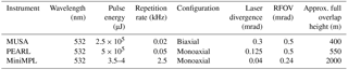
Table 2Specifications of MUSA and PEARL at 1064 nm, CL51 and CS135. All the instruments are operated in the zenith-pointing mode. RFOV indicates the half-angle rectangular field of view of the instruments.
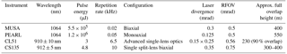
Ceilometers were installed on the roof of the observatory building (about 10 m above the ground), while the MiniMPL, being heavier and larger than a ceilometer, was deployed close to MUSA and PEARL at the surface. Table 1 reports MiniMPL, MUSA and PEARL specifications at 532 nm, while Table 2 shows specifications of the ceilometer infrared receivers, MUSA and PEARL.
MUSA is a mobile multi-wavelength lidar system, based on a Nd:YAG laser source emitting at 1064, 532 and 355 nm. The receiver unit consists of a Cassegrain telescope with a primary mirror of 300 mm diameter. The three laser beams are simultaneously and coaxially transmitted into the atmosphere beside the receiver in biaxial configuration. The receiving system has three channels to detect the elastically backscattered radiation from the atmosphere and two additional channels to detect the inelastically backscattered Raman radiation by atmospheric N2 molecules at 607 and 387 nm, respectively. The elastic channel at 532 nm is split into parallel and perpendicular polarization components by means of a polarizing beam splitter cube. The backscattered radiation at all the wavelengths is acquired by photomultiplier tubes in both analog and photon-counting mode. The calibration of depolarization channels is automatically made using the ±45 method (Freudhentaler et al., 2009). The typical vertical resolution of the raw profiles is 3.75 m at 1 min temporal resolution. The MUSA system is compact and transportable and it is one of the reference systems employed for the EARLINET quality assurance program. MUSA is routinely tested with respect to several systematic quality-assurance tests developed in order to harmonize the lidar measurements, setting up high-quality standards and improving the lidar data evaluation (Pappalardo et al., 2014). MUSA signals are also routinely evaluated using the Rayleigh fit test and signal-to-noise analysis (Baars et al., 2016). Additionally, the telecover test (Freudenthaler, 2008) is performed regularly and especially after transportation of the system. The system is aligned using a CCD camera to reduce the effect of misalignment between the telescope and laser axis, being MUSA a bistatic lidar. Finally, the multi-wavelength detection capability enables the so-called “3 + 2” lidar data analysis which, taking advantage of the simultaneous retrieval of aerosol extensive (extinction coefficients at 355 and 532 nm; backscattering coefficients at 355, 532 and 1064 nm) and intensive optical properties (lidar ratios at 355 and 532 nm and color ratios) at different wavelengths, permits to check the physical consistency of the retrieved aerosol properties.
The multi-wavelength lidar system for tropospheric aerosol characterization, PEARL, has been designed to provide simultaneous multi-wavelength aerosol measurements for the retrieval of optical and microphysical properties of atmospheric particles as well as water vapor mixing ratio profiles. The system, operated according to regular EARLINET measurement schedule until 2014, is presently used only for testing, during special events and as backup of MUSA system when MUSA was moved abroad for the calibration of the EARLINET stations (Wandinger et al., 2016). PEARL is based on a 50 Hz Nd:YAG laser source emitting at 1064, doubled and tripled to 532 and 355 nm, respectively. An optical system based on mirrors, dichroic mirrors and 2× beam expander separates the three wavelengths, allowing optimization of the energy and divergence for each wavelength. The beams are mixed again for collinearity of the three wavelengths and transmitted simultaneously and coaxially with respect to the lidar receiver. The backscattered radiation from the atmosphere is collected by an F/10 Cassegrain telescope (0.5 m diameter, 5 m focal length) and forwarded to the receiving system, where three channels detect the radiation elastically backscattered from the atmosphere at the three laser wavelengths and three channels are used for the Raman radiation backscattered from the atmospheric N2 molecules at 387 and 607 nm and from H2O molecules at 407 nm. Two additional channels detect the polarized components of the 532 nm backscattered light. Each of these channels is further split into two channels differently attenuated for the simultaneous detection of the radiation backscattered from the low- and high-altitude ranges, in order to extend and optimize the signal dynamic range. For the elastic backscattered radiation at 1064 nm the detection is performed by using an avalanche photodiode (APD) detector and the acquisition is performed in analog mode. For all the other acquisition channels, the detection is performed by means of photomultipliers and the acquisition is in photon-counting mode. The vertical resolution of the raw profiles is 7.5 m for 1064 nm and 15 m for the other wavelengths, and the raw temporal resolution is 1 min. PEARL measurements were extensively intercompared with MUSA to have a redundant aerosol profiling capability at CIAO.
The MiniMPL transceiver weighs 13 kg and measures 380 mm × 305 mm × 480 mm (width, depth and height). The system consists of a laptop and the lidar transceiver, connected by a USB cable, and the average power consumption is about 100 W during normal operations. The whole system fits in a transportable storm case with a telescopic handle and wheels and can be checked in as regular luggage during a domestic or international flight. The MiniMPL's Nd:YAG laser emits polarized 532 nm light at a 2.5 kHz repetition rate and 3.5–4 µJ nominal pulse energy. The laser beam is expanded to the size of the telescope aperture (80 mm) to satisfy the eye-safe requirements in ANSI Z136.1.2000 and IEC 60825 standards. The system also has built-in depolarization measurement (Flynn et al., 2007) with a contrast ratio greater than 100:1. The receiver uses a pair of narrowband filters with bandwidth less than 200 pm to reject the majority of solar background noise. The filtered light is then collected by a 100 µm multi-mode fiber and fed into a Silicon Avalanche Photodetector operating in photon-counting mode (Geiger mode). Photon-counting detection enables the MiniMPL design to be lightweight and compact with high SNR throughout the troposphere. MiniMPL sets the laser beam divergence at about 40 µrad and receiver field-of-view at 240 µrad. This design balances the solar noise with optical system stability and avoids multiple scattering which can distort measurements of depolarization ratio and extinction coefficient in the cloud.
The Vaisala Ceilometer CL51, the second generation of Vaisala single-lens ceilometers, is designed to measure high-range cirrus cloud base heights while maintaining the capability to measure low- and middle-range clouds and, in high turbidity conditions, to diagnose vertical visibility. Its application to detection of tropospheric aerosol layers is under investigation in several papers in literature (e.g., Wiegner et al., 2014). The CL51 employs a pulsed diode laser source emitting at 910 ± 10 nm (at 25 ∘C with a drift of 0.27 nm K−1) with a repetition rate of 6.5 kHz. The refractor telescope, which employs an enhanced single-lens technology, theoretically allows reliable measurements virtually at the surface, although the overlap correction estimated by the manufacturer is not able to effectively correct the ceilometer profile over the entire incomplete overlap region. The backscattered radiation is filtered using an optical bandpass filter which, according to Vaisala, is on the order of 3.4 nm and then detected using an APD in analog mode. The instrument used in INTERACT-II was updated with the latest firmware version (v1.034).
The Campbell Scientific CS135 ceilometer employs a pulsed diode laser source emitting at 912 ± 5 nm with a repetition rate of 10 kHz. The ceilometer receiver is based on a single-lens telescope. Half of the lens is used for the transmitter and the other for the receiver with a total optical isolation between them. The optical layout is conceived to enable lower-altitude measurement and to integrate larger optics into a compact package. Like the CL51, the backscattered radiation is filtered using an optical bandpass filter (36 nm) and detected using an APD in analog mode. The latest version of the instrument firmware was provided by the manufacturer itself. During INTERACT-II, CS135 data collection (performed using a terminal emulator) was affected by a technical problem with the CIAO logging system, which caused the loss of a large amount of data, especially in the free troposphere, thus limiting the number of available cases for the comparison (only nine measurement sessions).
At this stage, it is worth providing a few clarifications about the hybrid nature of this intercomparison campaign which involved both automatic elastic (polarized) lidars and regular ceilometers. As remarked upon in Madonna et al. (2015), ceilometers are optical instruments based on the lidar principle, but eye-safe and generally lower in cost and performance compared to advanced research or automatic elastic lidars. Their primary application is the cloud base height determination and vertical visibility for transport-related meteorology applications. These instruments typically have considerably lower SNRs than lidars because they employ diode lasers and wider optical bandpass filters to detect over the broader spectrum of these sources. Diode lasers sources are employed only if compliant with eye-safety requirements which permit ceilometers to be operated unattended. In a few more powerful ceilometers, like the CHM15k and CHM15kx, as well as the MPLs (including MiniMPL), the use of diode-pumped lasers allows much larger SNRs and, therefore, enhanced performances (e.g., Madonna et al., 2014). Moreover, ceilometers, while providing factory-calibrated attenuated backscatter profiles, do not often provide the raw backscattered signals and their processing software includes several automatic adjustments of the instrument parameters (e.g., gain, voltages, background suppression) performed according the observed scenario (e.g., daytime, nighttime, clear or cloudy sky) but out of the control of users. This makes it difficult to use them for research purposes beyond the applications for which they were designed.
During INTERACT-II, a hybrid ensemble of these instruments, automatic lidars and ceilometers have been deployed. Nevertheless, the main scope of the campaign remains to assess the performances of each different category of instruments separately and, within the same category, to assess the limitation in the use of each system involved. Therefore, the results presented in Sects. 4 and 5 are intended to show under which limitations each of the investigated systems is able to provide quantitative information on the aerosol properties in both the boundary layer and in the free troposphere. The reader should use these results according to his or her own specific needs and with careful consideration of the application.
Following the same approach used during INTERACT, CIAO lidar signals have been processed using the EARLINET Single Calculus Chain (SCC) (D'Amico et al., 2016; Mattis et al., 2016). The SCC outputs are the pre-processed RCSs and the profiles of aerosol extinction coefficient at 355 and 532 nm and backscattering coefficient at 355, 532 and 1064 nm, using both Raman and elastic signals. RCS is defined as the product of the pre-processed signal (background subtracted) multiplied by the square of the altitude range: RCS = P(z)z2, where P(z) is the lidar pre-processed signal and z is the altitude range for a zenith-pointing lidar.
In contrast with the ceilometers, the MiniMPL provides the raw signals acquired in photon-counting mode only, enabling the direct comparison with the CIAO lidar signals. RCS is a quantity proportional to the attenuated backscattering β′, which is used for the investigation of ceilometer performance and is defined as
where CL is the lidar constant (depending only on the lidar experimental setup), β(z) is the total (aerosol plus molecular) backscattering coefficient and T2(z) is the two-way transmissivity of the atmosphere. The use of RCSs allows a comparison between the two systems over a vertical range larger than the range where β′ is available. This is because the β′ calculation depends on the range covered by the retrieval of the CIAO lidar extinction coefficient using the Raman method, applied in this work. The lower SNR typical of the Raman lidar channels does not allow to provide a vertical profile of the aerosol extinction coefficient over the entire range typically covered by an elastic lidar signal. The use of RCSs brings the comparison to the signal level, avoiding calculation of higher level products, whose retrieval can increase the number of assumptions and uncertainties (e.g., Lolli et al., 2017).
To perform the comparison between CIAO lidars and MiniMPL, 532 nm MiniMPL RCS is normalized to the corresponding CIAO lidar RCS, on a profile-per-profile basis, over a vertical range of 1.2 km starting from a variable reference altitude between 6 and 8 , where the identified aerosol content is qualitatively negligible using quicklooks of the lidar time series. All the time series considered in this comparison refer to nighttime clear-sky measurements. The profiles from all the instruments are compared over a vertical resolution of 60 m and a temporal integration time ranging from 1 to 2 h, selected automatically by the SCC depending on the observed atmospheric scenario. No vertical smoothing is applied to the data, but systems outputting data at a higher resolution are interpolated to the CIAO lidar resolution. All of the profiles are cut in the lower part of the atmosphere, below 1300 , in order to consider CIAO lidar reference lidar signals only in the region with the full overlap between the telescope and laser beam. The number of the simultaneous CIAO lidars and MiniMPL measurements time series has been limited by a few periods of unavailability of the MiniMPL due to an issue in the regulation of the instrument housing temperature.
Regarding the ceilometers, the comparison was carried out using the 1064 nm β′ profiles obtained through their normalization over the corresponding CIAO lidar β′ profile below 3 , over a vertical range of 600 m, where the full overlap of all instruments was ensured. Given that ceilometer measurements are performed at 910–912 nm, β′ profiles have been rescaled using the 532∕1064 backscatter-related Ångström coefficient measured by CIAO lidars in order to obtain the equivalent profile at 1064 nm for comparison with CIAO lidars. For those altitudes where the backscatter-related Ångström coefficient was not available (typically in the free troposphere (FT), above 5 ) a climatological value of 1.05 was used. The uncertainty contribution for the spectral dependence of β′ and, therefore, of the aerosol backscattering coefficient and of molecular and aerosol extinction coefficients has been estimated within a few percents. More details on calibration are discussed in Sect. 5.
A ceilometer β′ profile can only be retrieved if water vapor absorption is taken into account (Wiegner et al., 2015). The influence of water vapor absorption at operating wavelengths of ceilometers is due to the presence of a strong absorption band between 900 and 930 nm, while at 1064 nm there is no absorption. Therefore, the retrieval of β′ profiles must consider the attenuation of the backscattered radiation by water vapor. In this study, the method used for correcting the attenuation by water vapor is based on the Fu–Liou–Gu (FLG) radiative transfer model (Gu et al., 2011), in the modified version discussed in Lolli et al. (2018).
FLG is a combination of the delta four-stream approximation for solar flux calculations (Liou, 1986) and a delta two–four-stream approximation for IR flux calculations. The solar (0–4 µm) and IR (4–50 µm) spectra are divided into 6 and 12 bands, respectively, according to the location of prominent atmospheric absorption bands. FLG makes use of the adding procedure to compute the spectral albedo in which the line-by-line equivalent radiative transfer model (Liou et al., 1998) uses the correlated K-distribution method for the sorting of absorption lines in the solar spectrum. In the solar spectrum, non-gray absorption due to water vapor, O3, CO2, O2 and other minor gases, such as CO, CH4 and N2O, is taken into account. Non-gray absorption due to water vapor, O3, CO2, CH4, N2O and CFCs is considered in the IR spectrum. Potenza GRUAN (GCOS Research Upper-Air Network) processed (collocated) radiosoundings were used as input for the FLG radiative transfer model (Lolli et al., 2017) in about 40 % of the cases, while for the remaining cases, when local radiosoundings were not available, data from closest RAOB (the Universal RAwinsonde OBservation program) site located in Brindisi Casale (40.63∘ N, 17.94∘ E; 15 m), about 150 km east of Potenza, were used. RAOB profiles were cut at the CIAO altitude level (760 m). According to the correction method suggested in literature for 905–910 nm ceilometers (Wiegner et al., 2015), an optimal correction would require the knowledge of both the laser wavelength and the bandwidth for each emitted pulse. These data are not currently stored and provided by the ceilometer hardware. Therefore, to estimate the water vapor correction a laser Gaussian profile centered at the nominal laser wavelength with FWHM (full width at half maximum) of 3.5 nm has been assumed. Moreover, FLG has a spectral resolution of 50 cm−1, while in literature a resolution lower than 0.2 cm−1 is recommended to avoid an “unpredictable” behavior of the model calculation. The water vapor absorption has been calculated through the average absorption within the spectral range described above. In addition, the comparison between the ceilometers and the lidars, discussed in Sect. 5, shows that the uncertainty due to the water vapor correction cannot represent the main contribution to the total uncertainty budget of 905–910 nm ceilometer measurements.
For the comparison between CIAO lidars and MiniMPL, it is important to remark that MUSA detects with two channels the co- and cross-polarized components of the elastically backscattered radiation at 532 nm, in order to measure the particle depolarization at that wavelength. MiniMPL also detects the co- and cross-polarized components of the elastically backscattered radiation at 532 nm and provides continuous measurements of particle backscattering coefficient and depolarization ratio profiles. Because of different polarization setups, MUSA measures the particle linear depolarization ratio (Freudenthaler et al., 2009) while MiniMPL measures the particle circular depolarization (Flynn et al., 2007). For both MUSA and MiniMPL, total signals must be calculated for through the combination of the respective co- and cross-polarized channels. 532 nm MiniMPL RCS has been calculated according to the equations provided in Campbell et al. (2002). PEARL, instead, is equipped not only with the co- and cross-polarized channels at 532 nm but also with channels detecting the 532 nm total backscattered radiation.
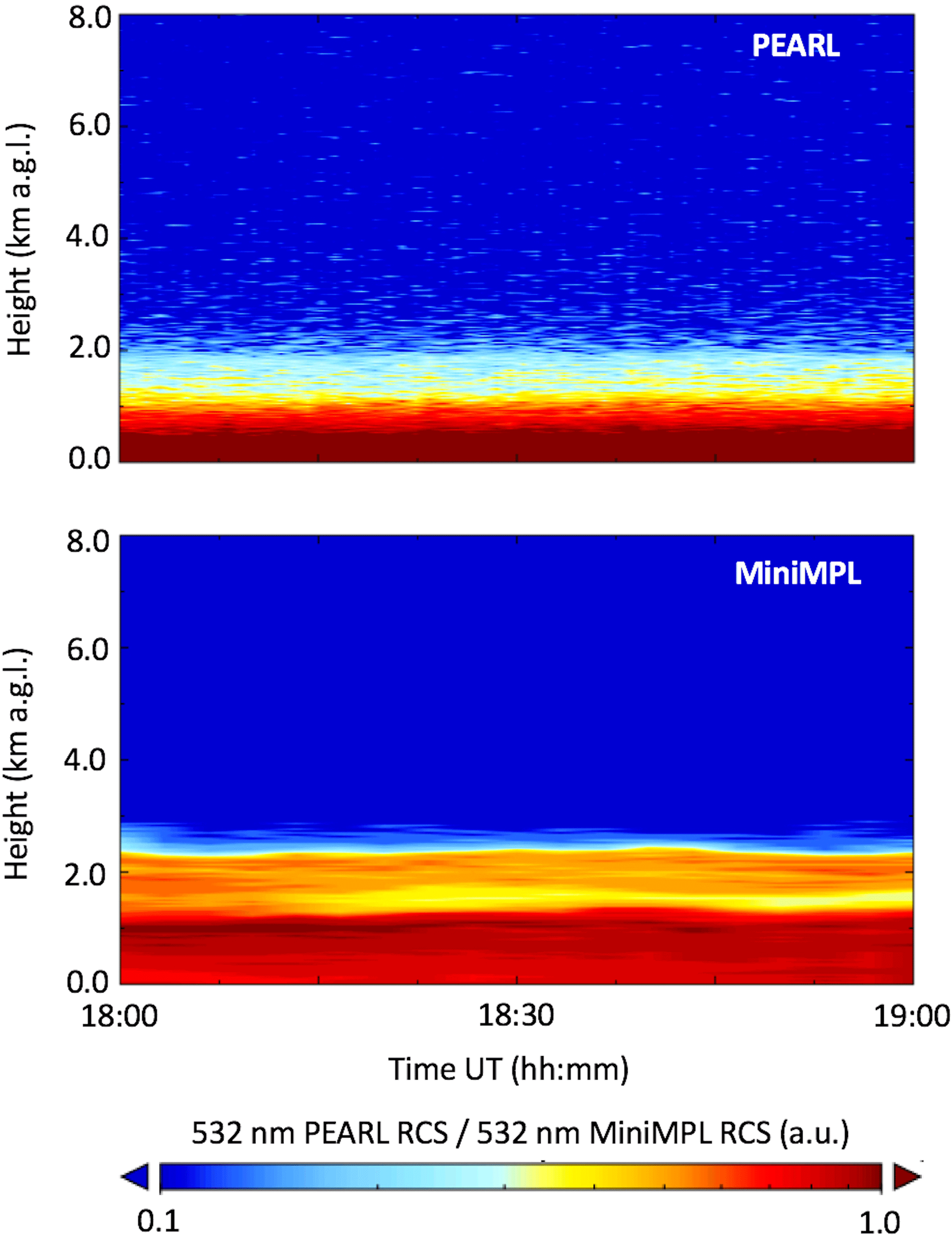
Figure 1Time series of 532 nm range-corrected signal (RCS) measured with PEARL and MiniMPL on 13 October 2016 from 18:00 to 19:00 UT; heights are above ground level (a.g.l.); raw time and vertical resolutions are 1 min and 15 m for PEARL and 5 min and 30 m for MiniMPL. The color scale shown at the bottom is logarithmic.
To provide a first example related to the dataset discussed in this paper, a comparison of the 532 nm PEARL RCS and MiniMPL RCS (not normalized) at their own time and vertical raw resolutions is shown in Fig. 1 for the measurements collected on 13 October 2016 from 18:00 to 19:00 UT. Figure 2 shows the comparison of the 1064 nm PEARL RCS with the 910–912 nm CL51/CS135 attenuated backscatter for the same day. To ensure correct interpretation of Figs. 1 and 2, it is important to reiterate that raw time and vertical resolutions are 1 min and 15 m for PEARL, 5 min and 30 m for MiniMPL, 30 s and 10 m for CL51 and 30 s and 5 m for CS135.
Finally, it is also important to note that the CIAO operator routinely checked each instrument during INTERACT-II to ensure that each one was performing according to the manufacture specifications. The routine maintenance included the following:
- a.
A daily inspection was made of each instrument and its operation.
- b.
A weekly check was performed on each instrument's acquisition parameters (laser transmitter, receiver, heater, blower, windows, tilt angle, etc.).
- c.
Windows were cleaned approximately biweekly, with frequency depending on atmospheric conditions (e.g., after precipitation or dust/smoke transport events), using the flooding method. Additionally, specific treatments to remove the stronger dust spots were performed in response to warning messages provided by each instrument (e.g., window contamination messages).
- d.
Dark current measurements were made twice during the campaign for ceilometers, using a termination hood provided by the manufacturer while operating in analog detection mode. Dark current profiles were subtracted from each of the raw backscatter profiles before normalization using the lidar; for MUSA and PEARL, dark currents were routinely estimated before each measurements session.
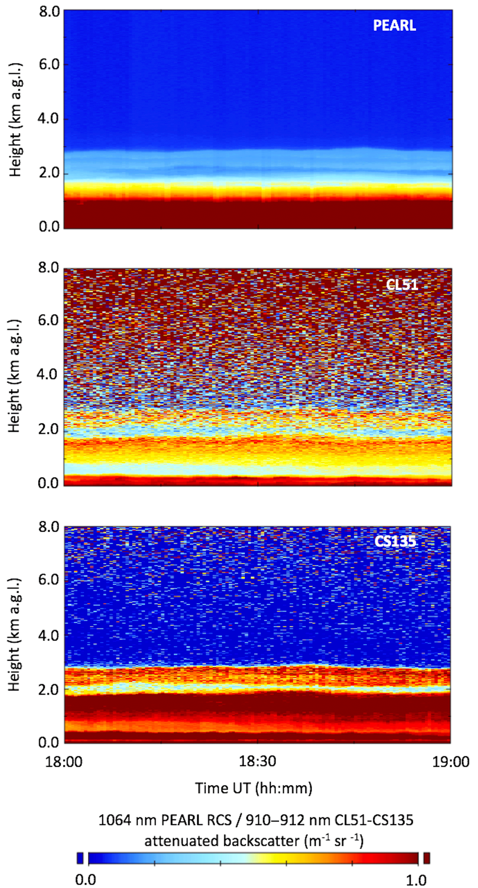
Figure 2Time series of 1064 nm PEARL RCS and 910–912 nm CL51 and CS135 attenuated backscatter profiles as provided by the manufacturer software for the measurements collected on 13 October 2016 from 18:00 to 19:00 UT; heights are above ground level (a.g.l.); raw time and vertical resolutions are 1 min and 7.5 m for PEARL, 30 s and 10 m for CL51 and 30 s and 5 m for CS135.
Simultaneous observations of aerosol collected with the multi-wavelength Raman lidars operative at CIAO, MUSA and PEARL and of the automatic Sigma Space MiniMPL, collected during the measurement campaign, have been compared.
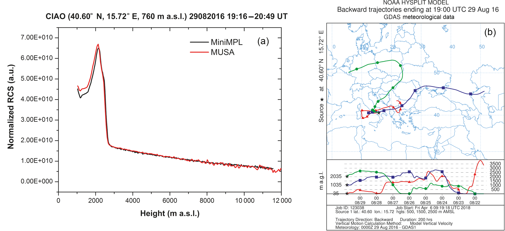
Figure 3(a) Comparison between RCS profiles obtained from MUSA and MiniMPL on 29 August 2016 from 19:16 to 20:47 UT; (b) the corresponding air mass back-trajectory analysis performed using NOAA HYSPLIT model. HYSPLIT simulations have been initialized at the three levels from the ground to the top height of the highest layer observed by both MUSA and MiniMPL.
An example of comparison between RCS provided by MUSA and MiniMPL is shown in Fig. 3a, related to the observations collected on 29 August 2016 from 19:16 to 20:47 UT. The quicklooks of the RCS time series (not reported) show a sharp aerosol layer between about 1.5 km and 2.5 along with a lower RCS below the layer to the ground, while the atmosphere is dominated by the molecular scattering above. In Fig. 3b, the air mass back-trajectory analysis performed using the NOAA HYSPLIT (Hybrid Single Particle Lagrangian Integrated Trajectory) model (Stein et al., 2015) initialized at three levels from the ground to the top height of the highest layer observed by both MUSA and MiniMPL. Trajectories are obtained using the vertical velocity model of HYSPLIT running the back trajectories for a length of 200 h at three vertical levels.
The difference between the two profiles shows a good agreement throughout the troposphere with discrepancies < 5 % between 2.0 and 4.0 , within the RCS random uncertainty (D'Amico et al., 2016). MiniMPL underestimates MUSA (up to 10 % RCS) at altitudes lower than 2.0 , in the incomplete overlap region. MiniMPL data processing provides a correction function which is not able to properly adjust all of the collected signals in the incomplete overlap region. The beam pointing instability of the laser in this vertical range is likely the reason preventing the adjustment using a precomputed static correction function.
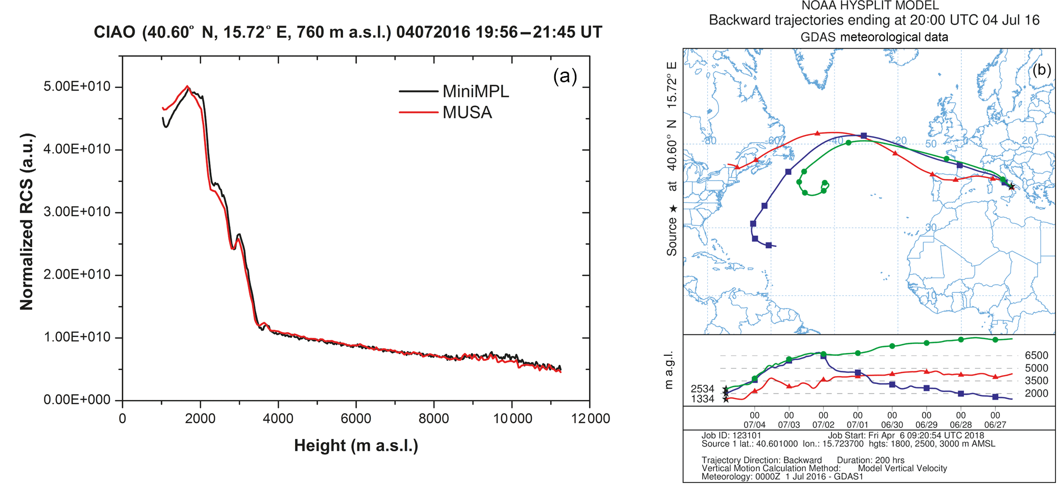
Figure 4(a) Same as Fig. 3a but obtained from MUSA and MiniMPL on 4 July 2016 from 19:56 to 21:45 UT. (b) Same as Fig. 3b; the corresponding air mass back-trajectory analysis performed using NOAA HYSPLIT model is reported.
A second example (Fig. 4a) shows MUSA and MiniMPL RCS values collected on 4 July 2016 from 19:56 to 21:45 UT. Multiple aerosol layers up to 4.0 are observed. In Fig. 4b, the corresponding air mass back-trajectory analysis shows the quasi-zonal transport of the observed aerosol from northeastern Canada over the Atlantic Ocean to Europe. Also in this case, the comparison shows a good agreement throughout the troposphere with discrepancies < 5 %, which are identified both in the incomplete overlap region and above this region and up to 4.0 km of altitude, where most of the aerosol loading is located. This might be related to the uncertainty affecting the estimation of corrections other than overlap applied to the MiniMPL data processing, e.g., after-pulse correction. The manufacturer shall investigate this hypothesis. Nevertheless, the discrepancies are within the RCS random uncertainty and do not compromise the good agreement between the two systems.
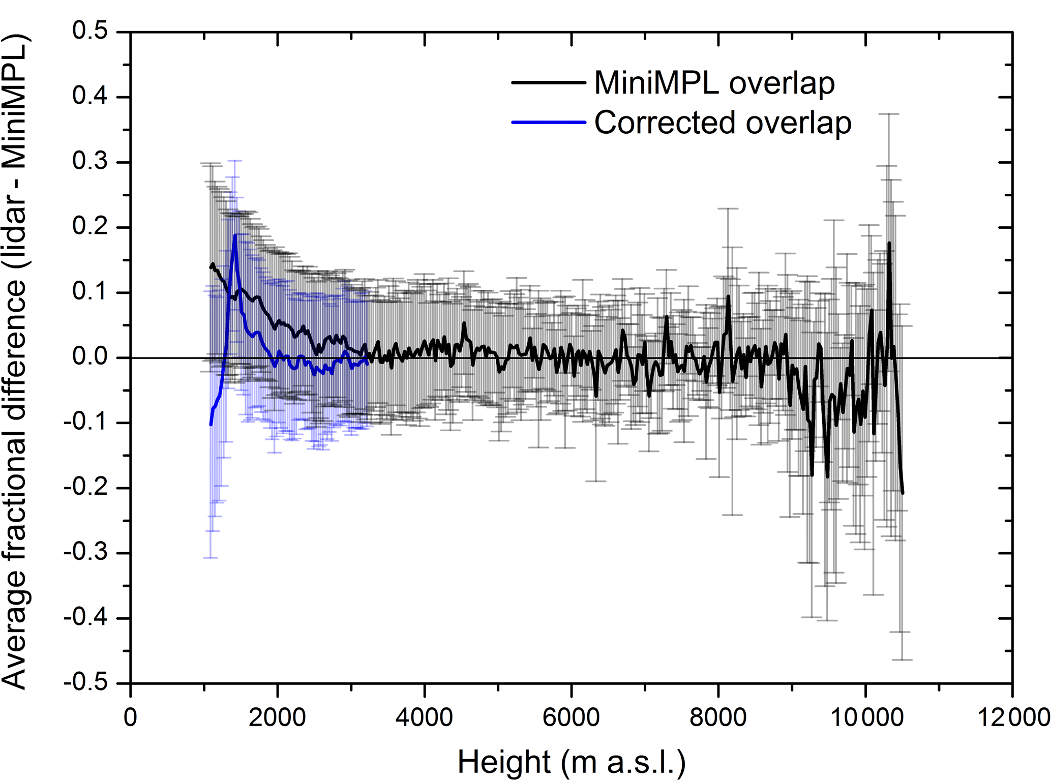
Figure 5Profiles of the average fractional difference between MUSA and MiniMPL values of RCS calculated on 12 cases of simultaneous and collocated measurements (black line). Blue line is the same as black line but applying an additional overlap correction factor to the MiniMPL data processing estimated using the ratio between MUSA and MiniMPL profiles during the cleanest simultaneous measurement session available during INTERACT-II. The vertical bars are the SDs of fractional difference.
In Fig. 5, the black line shows the profile of the average fractional difference between CIAO lidar and MiniMPL values of RCS calculated for 12 cases of simultaneous and collocated measurements collected in the period from July to December 2016. The vertical bars are the SDs of fractional differences. Fractional difference is defined as the relative difference between CIAO lidar RCS and MiniMPL RCS values with respect to RCS normalized by CIAO lidar. The profile shows that MiniMPL underestimates CIAO lidar MUSA in the region below 2.0 km with an increasing average fractional difference towards ground level; the maximum value of this deviation is less than 15 %. The blue line reported in Fig. 5 represents the same as the black line but adjusted by applying an additional overlap correction factor to the MiniMPL, estimated using the ratio between MUSA and MiniMPL RCS profiles during the cleanest simultaneous measurement session available during INTERACT-II. The additional correction applied from the ground to 3.3 , identified as the overlap height for the MiniMPL, reduces the average fractional difference in the range from 1.5 to 3.3 km, with values less than 3 % from 1.8 km and the SD of the difference keeps to within 10 %. Below 1.5 km, the correction is not able to properly adjust the profile due to the presence of the aerosol residual layer in the measurements used to estimate the correction factor. The example correction for the overlap effects provided in Fig. 5 cannot be considered exhaustive, but demonstrates that some work is required to improve the MiniMPL data processing in the incomplete overlap region. In the remainder of this section, the MiniMPL original data processing will be considered.
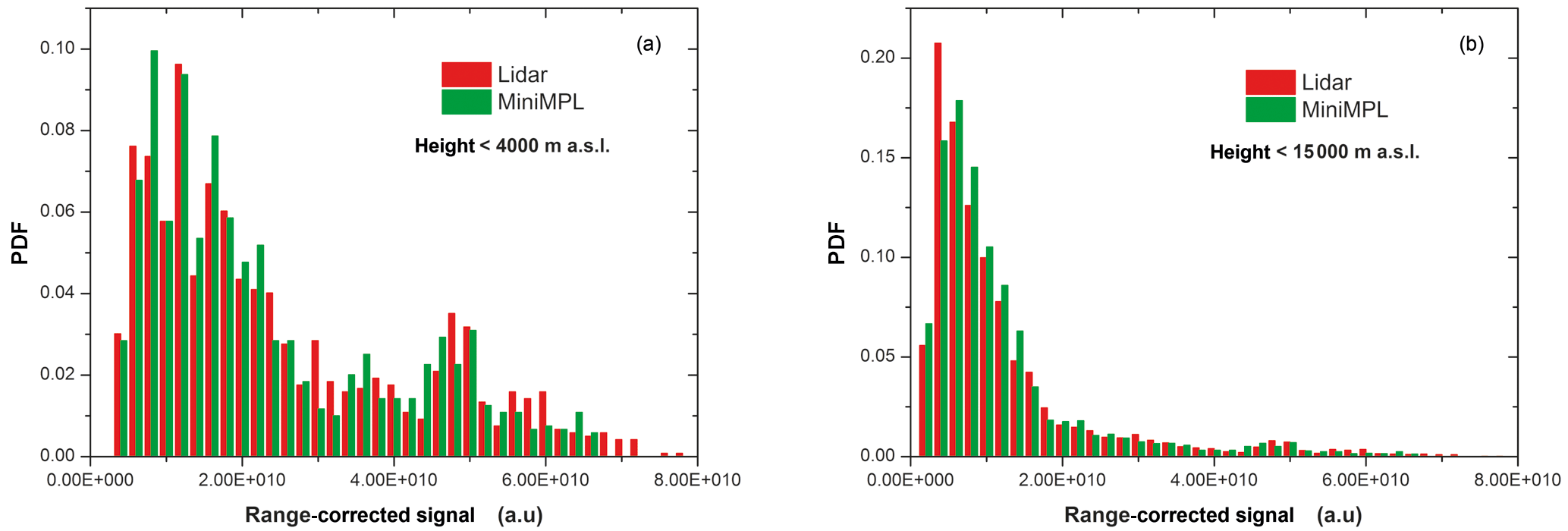
Figure 6(a) Probability density functions (PDFs) of the RCS values measured by CIAO lidars and MiniMPL below 4 km. (b) Same as (a) but for the entire vertical range of observed lidar profiles, below 15 km.
To evaluate the MiniMPL stability during the campaign, the values of the normalization constant were averaged during two different periods, one corresponding to MUSA used as reference and the other to PEARL, in order to assess a relative variability for the same constant. The normalization was typically performed between 6 and 8 Then the averaged relative variabilities calculated during these two different periods showed that the stability of the MiniMPL calibration (“lidar normalization”) during the campaign was within ±29 %. This value embeds the PEARL–MUSA system variability, which is evaluated from the molecular calibration constant, and it is within 20 % for both systems. However, given both the number of simultaneous observations available and the use of two lidar systems as the reference lidars in two different time periods, the estimation of the calibration stability must be handled with caution. In general, the MiniMPL showed a good stability in its operation during the considered time period and with respect to seasonal changes in the environmental temperature and in the aerosol loading.
In Fig. 6, the comparison of RCS values between CIAO lidars and MiniMPL probability density functions (PDFs) confirms the overall good agreement of the two instruments, with a tendency of MiniMPL to overestimate CIAO lidars for RCS values lower than 1.5 × 10¹⁰ (): this difference is more evident in Fig. 6a, where PDFs are calculated for the vertical range below 4.0
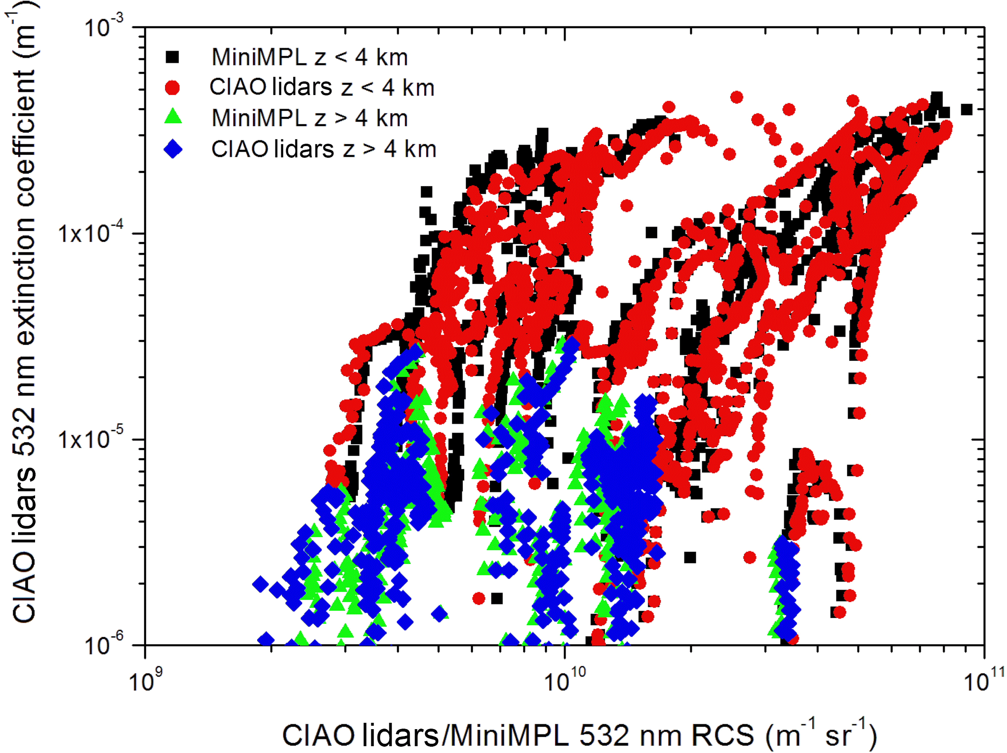
Figure 7Comparison of the scatter plots showing the relationship between CIAO lidars 532 nm aerosol extinction coefficient and MiniMPL and CIAO lidars 532 nm RCS. Black squares are the values of MiniMPL measured below 4 km, green triangles are the values of MiniMPL measured above 4 km, red squares are the values of CIAO lidars measured below 4 km and blue diamonds are the values of CIAO lidars measured above 4 km.
Finally, in Fig. 7, the relationships between the 532 nm aerosol (particle) extinction coefficient (αpar) from MUSA and PEARL lidars and the corresponding RCS at 532 nm measured by MUSA and PEARL lidars and by MiniMPL are shown to highlight differences in lidar sensitivity to different aerosol extinction coefficients. αpar is calculated over the same temporal window as RCS, but with a lower effective vertical resolution (typically within 480–600 m) in order to reduce the uncertainty and the related oscillation affecting the extinction profile calculated using the Raman lidar signal. The output profile vertical resolution is 60 m to match the RCS vertical resolution. The comparison in Fig. 7 shows a good agreement between MiniMPL and CIAO lidars. Small differences can be identified and are more evident for αpar values larger than about 5.0 × 10⁻⁵ m−1, where MiniMPL RCS values are more scattered compared to CIAO lidars. The RCS differences may be the results of systematic effects due to inaccurate adjustments applied to the signal processing, including the incomplete overlap correction, which for MiniMPL looks quite relevant in the region between 1.0 and 3.3
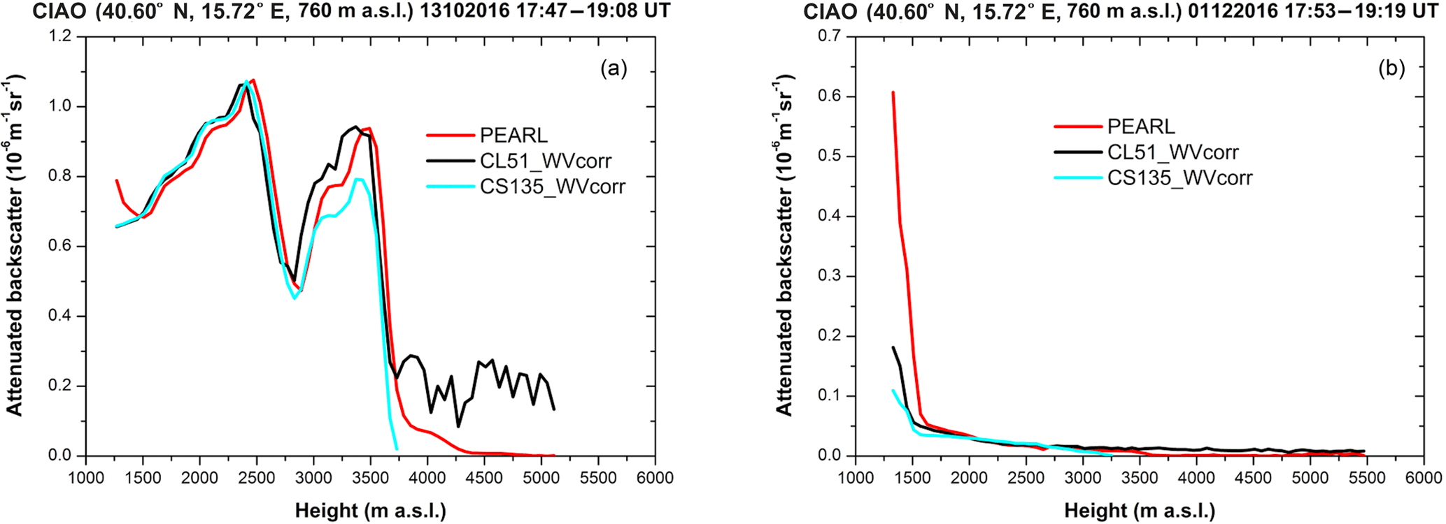
Figure 8(a) Comparison between the attenuated backscatter profiles retrieved from PEARL, CL51 and CS135 on 13 October 2016 in the time interval from 17:47 to 19:08 UT and obtained normalizing the ceilometer profiles on the PEARL profile in the region between 1.8 and 3.0 km. (b) Same as (a), but for the 1 December 2016 in the time interval from 17:53 to 19:19 UT. All the ceilometer profiles are corrected for the water vapor absorption affecting the signal extinction at 910–912 nm.
This section focuses on the comparison of attenuated backscatter profiles (β′) simultaneously measured by MUSA and PEARL multi-wavelength Raman lidars and estimated for CL51 and CS135 ceilometers. Figure 8a shows the attenuated backscatter retrieved by PEARL, CL51 and CS135 on 13 October 2016 in the time interval from 17:47 to 19:08 UT. The HYSPLIT air mass back-trajectory analysis (not shown) reveals that the observed advected aerosol layers may come from Libya and Morocco, two regions where large sources of dust are present at the different altitude levels where aerosol layers are observed with MUSA. The agreement between the three instruments is extremely good below 2.5 Between 2.5 and 3.7 the differences are larger for both the CL51 and the CS135 (larger difference shown by CS135). The difference between the CL51 and CS135 in the region between 2.5 and 3.5 may be also partly affected by the dependency of the water vapor correction on the emitted laser spectrum. The CS135 signal strongly decreases above 3.5 km close to the top region of the second observed aerosol layer. The CL51 signal is higher but the noise suggests that it is not reliable to detect the residual aerosol backscattered radiation at that altitude range as well the molecular return. All the CL51 profiles shown in Fig. 8 are cut below 5.0 , to better visualize the comparison otherwise affected by the large noise oscillation of the signals.
Figure 8b shows attenuated backscatter measured by the same instruments on 1 December 2016 from 17:53 to 19:19 UT. The air mass back-trajectory analysis for this time period showed that the observed air mass originated in Canada and reached CIAO via northwestern Europe. This comparison reveals the effect of ceilometer variability in the region of incomplete overlap (Vande Hey et al., 2011): the correction applied by the manufacturer is often able to adjust the profile minimizing the difference with respect to the reference CIAO lidars, but in many other cases, as for 1 December, differences are considerable. It is worth reiterating that, as for the MiniMPL comparison, all the profiles are cut off below 1.3 because CIAO lidars are considered as a reference only in the full overlap region.
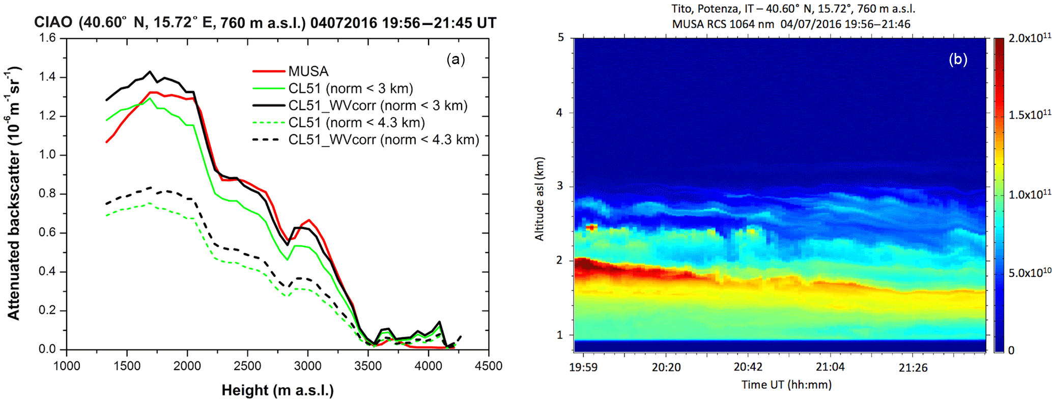
Figure 9(a) Comparison between the attenuated backscatter vertical profiles retrieved from MUSA and CL51 on 4 July 2016 from 19:56 to 21:45 UT and obtained using two different normalization ranges, the first below 3 km (solid lines) and the second below 4.3 km (dashed lines); both the raw calibrated profiles and the water vapor calibrated corrected profiles are shown. (b) Time series of the RCS measured with MUSA at 1064 nm during the same time period used to create the average profiles in panel (a).
Regarding the CL51 β′ profiles, normalization range choice has proven to be more critical than expected. Initially, all the CL51 profiles were normalized over a window of 0.6 km vertical range below 8 , in order to find a trade-off between an acceptable CL51 SNR and the need for normalizing in a stable aerosol-free region of the atmosphere. Nevertheless, the CL51 SNR is too low in the FT and the decrease in its sensitivity to the molecular return makes the normalization to the lidar in the FT (and consequently the ceilometer molecular calibration) challenging. Figure 9a shows the comparison between β′ retrieved from MUSA and CL51 on 4 July 2016 from 19:56 to 21:45 UT using two different normalization ranges, the first below 3 km and the second below 4.3 km, over a 0.6 km window normalization range. Both the raw calibrated profiles and the water vapor corrected calibrated profiles are shown. In Fig. 9b, the MUSA 1064 nm RCS time series measured during the same time is shown. The aerosol layer observed up to 3.5 is advected from a zonal transport above the Atlantic Ocean and then over Northern–Central Africa and likely includes transported mineral dust. The Fig. 9a comparison clearly reveals that, due to the very low SNR for the CL51 above 3.5 , the molecular calibration is challenging and may result in systematic errors on the retrieved profiles. Aside from the stratocumulus cloud calibration, not addressed in this work, the only possible CL51 normalization to provide reliable estimations of β′ must be performed over a profile of retrieved from a reference lidar (like MUSA or PEARL).
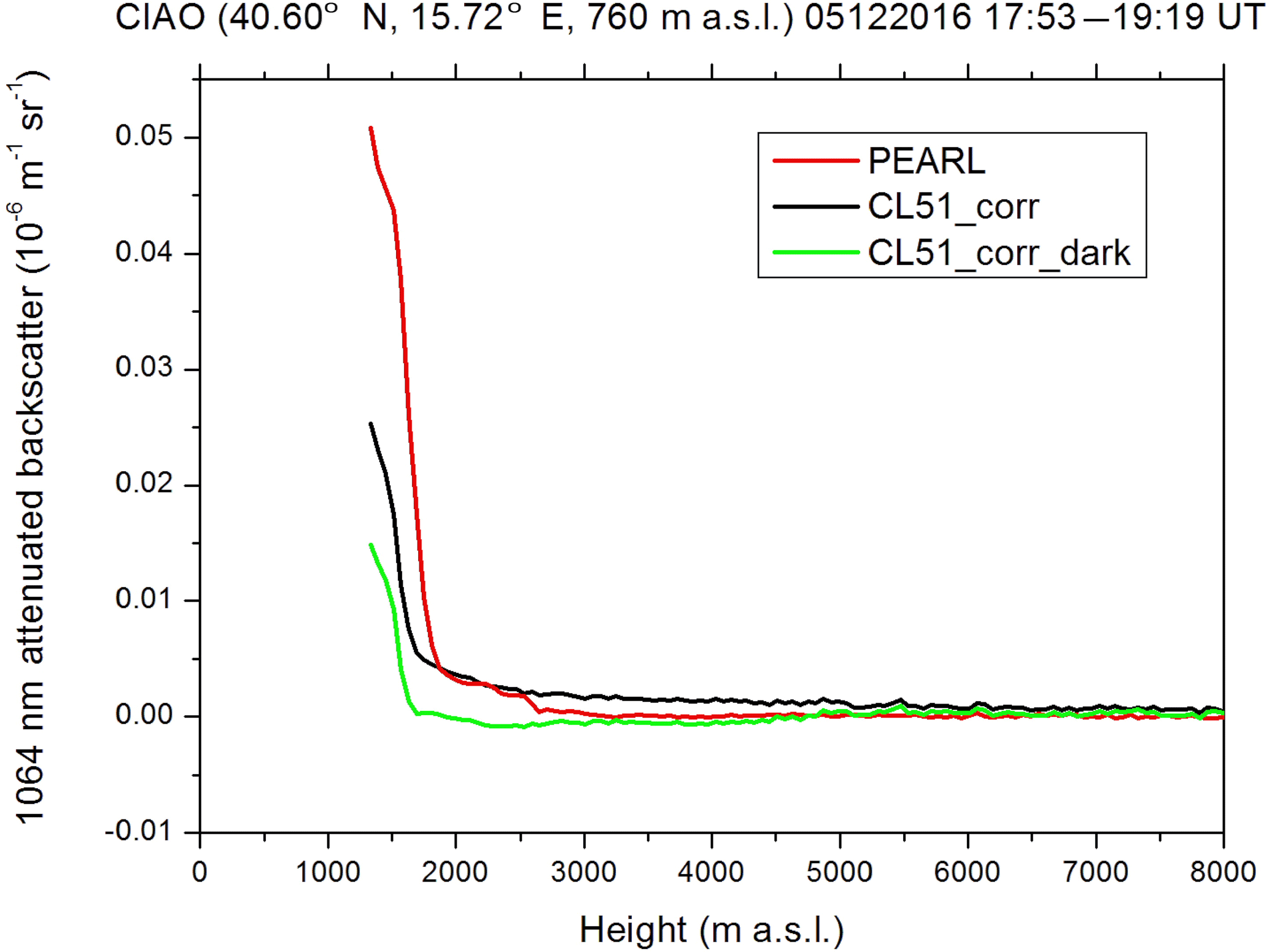
Figure 10Comparison among the attenuated backscatter profile retrieved from PEARL (red), from CL51 accounting for the water vapor absorption at its operating wavelength (dark) and from CL51 subtracting the dark current measured separately and then accounting for the water vapor absorption (blue) on 1 December 2016 in the time interval from 17:53 to 19:19 UT.
CL51 and CS135 dark currents were subtracted from each ceilometer vertical profile to subtract instrumental artifacts affecting the signals, especially in the free troposphere, and to test the feasibility of calibrating ceilometers using the molecular profile. In the CS135, the lack of information in the free troposphere due to data logging problems affected the measured dataset. For the CL51, dark current subtraction significantly reduces the distortions affecting the profiles in the free troposphere. Nevertheless, the ceilometer β′ profile calculated for 5 December 2016 from 17:53 to 19:19 UT (Fig. 10), after the dark current subtraction, still has large differences in shape with respect to the PEARL profile, which was successfully calibrated using a molecular profile. The comparison reveals that after dark current subtraction the CL51 β′ becomes negative between 2.0 and 4.5 , indicating that the measured dark currents are inadequate to correct for signal distortion along the entire profile. This kind of scenario is commonly found throughout the INTERACT-II dataset. 5 December 2016 was chosen because it was the closest clear-sky available date to the dark current measurements, taken on 22 December 2016.
It is worth clarifying that more frequent dark currents measurement over a longer temporal window could improve the correction of the signal distortion affecting the ceilometer β′ profiles in the free troposphere. Measuring the dark current every 12 h (once during nighttime and once during daytime), for 1–2 h, might enable successful application of the molecular calibration. The best practice for performing these measurements, though primarily of interest to the lidar research community, could be assessed for ceilometers in cooperation with the manufacturers in order to improve dark current correction and allow a more accurate molecular calibration. Tests to assess the value of performing appropriate dark measurements to enable the molecular calibration for the 905–912 nm ceilometers are currently under investigation through analysis of the database collected during the CeiLinEX Campaign (Mattis et al., 2017).
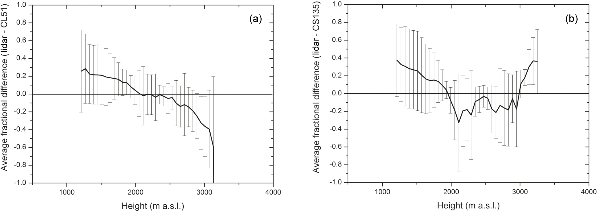
Figure 11(a) Profiles of the average fractional difference between CIAO lidars and CL51 values of the attenuated backscatter calculated for 19 cases of simultaneous and collocated measurements; (b) same as (a) but for CIAO lidars and CS135 calculated for nine cases. The vertical bars are the SDs of fractional differences.
Figure 11a shows the profile of the average fractional difference (defined in Sect. 4) between CIAO lidars and CL51 values of RCS calculated for 19 cases of simultaneous and collocated measurements, while panel b shows the same but for CS135 only for 9 cases. The vertical bars again represent the SDs of fractional differences. The profiles were cut off at about 3.5 for both ceilometers due to scarcity of available cases with a sufficient high SNR above that altitude. The CL51 underestimates CIAO lidars in the region below 2.0 with a difference up to 20–30 %. It overestimates CIAO lidars above 2.0 km, where the decrease of the CL51 SNR with altitude above 3.0 km does not allow the normalization in the FT and the differences with CIAO lidars increase to 40–50 %. In the region between 2.0 and 3.0 , where the normalization is applied, the difference is within 10 %. Using the same approach described in Sect. 4 for MiniMPL, the calculation of the CL51 normalization constant shows a variability within ±46 %. While CS135 performances are similar to the CL51 in the region below 3.0 , the difference between CS135 and CIAO lidars in the region above 3 ranges between ±40 %. The CS135 normalization constant ranges within ±47 %.

Figure 12PDFs of the attenuated backscatter values measured or estimated by CIAO lidars and CL51 (a) and by CIAO lidars and CS135 (b) below 4 km, respectively.
Figure 12 shows the PDFs of the β′ values measured or estimated by CIAO lidars and CL51, in panel a, and by CIAO lidars and CS135, in panel b. The PDFs are limited to β′ values below 4 due to the SNR decrease of both the instruments (see above). The intercomparison confirms the agreement between CIAO lidars and both ceilometers for the higher values of β′, while for lower values, below 0.2–0.3 10−6 , the differences are more pronounced due to the lower ceilometers' SNRs.
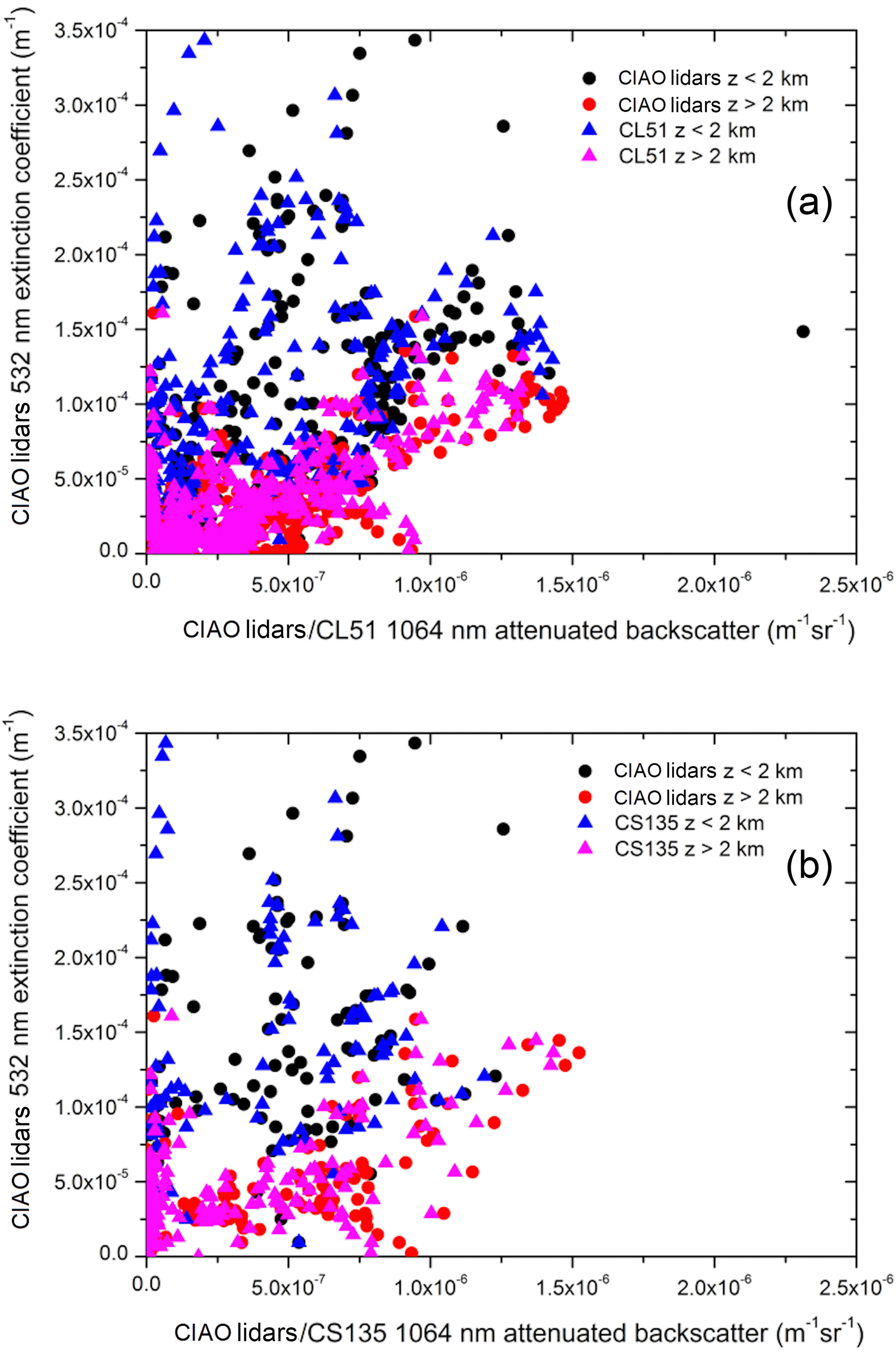
Figure 13Comparison of the scatter plots showing the 532 nm CIAO lidar aerosol extinction coefficient vs. 1064 nm attenuated backscatter from CIAO lidars and CL51 (a) and from CIAO lidars and CS135 (b). Black dots are the values of CIAO lidars measured below 2 km, red dots are the values of CIAO lidars measured above 2 km, blue triangles are the values of CL51/CS135 measured below 2 km and pink triangles are the values of CL51/CS135 measured above 2 km.
Finally, Fig. 13 shows the scatter plots of 532 nm aerosol extinction coefficient from CIAO lidars vs. 1064 nm attenuated backscatter from CIAO lidars and CL51 in panel a and from CIAO lidars and CS135 in panel b. The scatter plots include just the values measured below 3.5 For the CL51, differences with CIAO lidars in the scatter plot are small and mainly related to the region where β′ < 5.0 × 10⁻⁷ and αpar > 8.0 × 10⁻⁵ m−1: in this region, the values observed by CIAO lidars correspond to very small values detected by the CL51. For the CS135, though a small number of cases are available, a behavior similar to the CL51 can be identified in the region where β′ < 6.0 × 10⁻⁷ and αpar > 5.0 × 10⁻⁵ m−1; these threshold values reveal the slightly better performance of the CL51 when the values of αpar are larger for corresponding small values of β′. These values are measured within the nighttime aerosol residual layer, in particular below 2.0 , where the profiles measured by both the ceilometers may still be affected by the correction for the system's incomplete overlap.
In the previous sections, the overall stability of ceilometers' calibration constant calculated in this paper has been addressed in a statistical sense. The use of two different multi-wavelength Raman lidars during INTERACT-II did not permit evaluation of the stability of the ceilometer calibration constant in comparison with the lidar system molecular calibration constant, nor did it permit in depth assessment of calibration stability in relation to other parameters (e.g., ambient temperature, aerosol optical depth). Though MUSA and PEARL lidars were compared in the past and may be used almost interchangeably to measure aerosol optical properties, their experimental setups are quite different and therefore different calibration constants are required for the two systems.
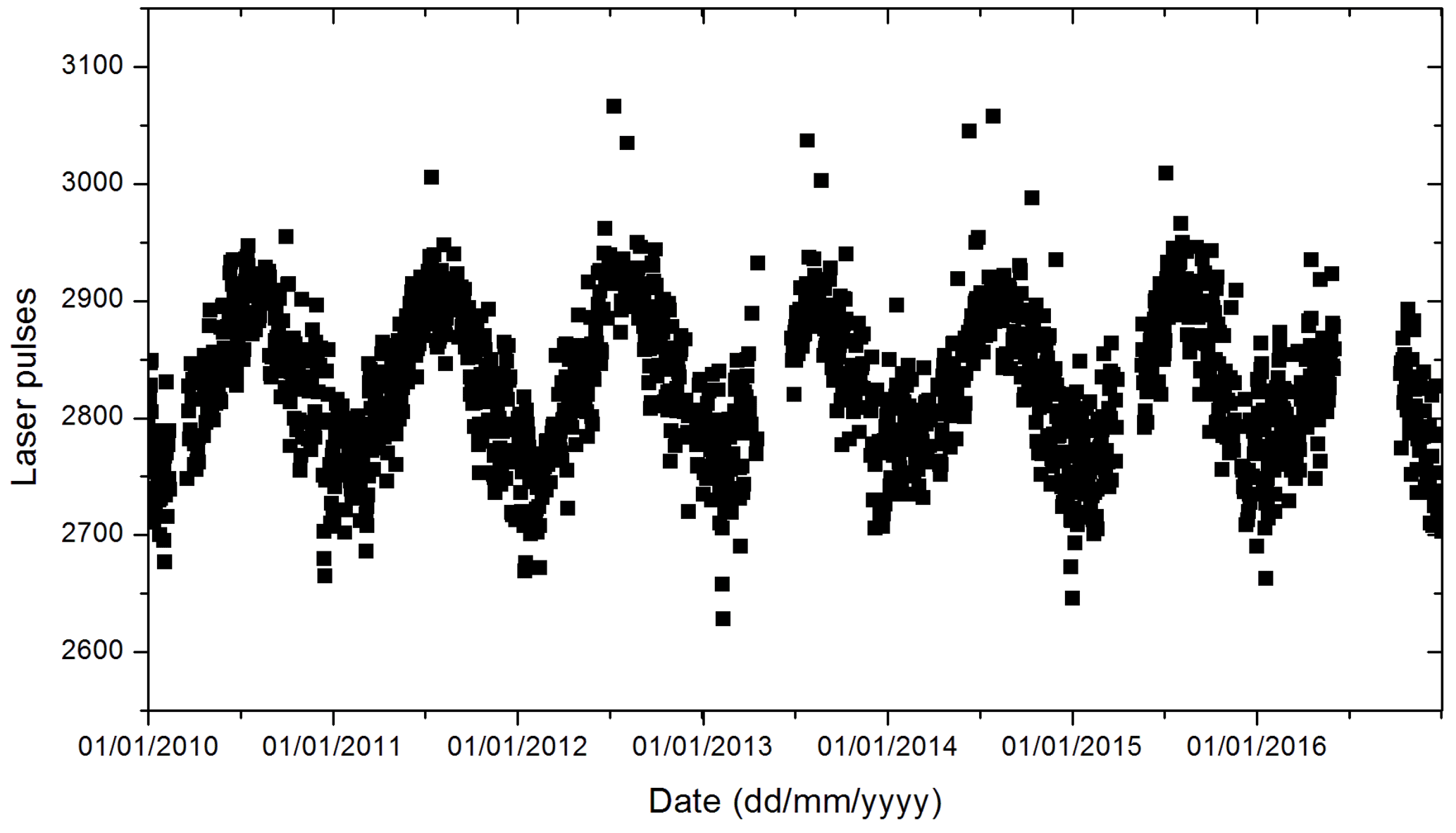
Figure 14Number of laser pulses hourly emitted by the CHM15k as a function of the time for the measurement period from 2010 to 2016.
Nevertheless, following on the INTERACT results and in order to assess stability of ceilometer calibration over time, a few tests and studies were performed using the CHM15k as a test bed. The system (already successfully tested during INTERACT) was not available for much of INTERACT-II due to major maintenance from July to October 2016; therefore it was devoted to this auxiliary testing role, taking advantage of the ancillary information provided by the manufacturer through the CHM15k acquisition software. Few tests revealed non-negligible sensitivity of the laser to changes in the ceilometer's enclosure temperature. These changes affect the number of laser pulses emitted per measurement cycle and they are correlated with changes in ambient temperature. To investigate the effect of this behavior on the ceilometer data processing, the whole CHM15k historical dataset available at CIAO was investigated. In particular, in Fig. 14 the number of laser pulses hourly emitted by the CHM15k is shown as a function of time from 2010 to 2016. The number of plotted points in Fig. 14 has been limited anyway to enable a good visualization. The CHM15k laser specifications provided by the manufacturer are consistent with the measured laser pulse variability, less than < 10 %. Occasionally, values of the laser pulses' variability up to 15–20 % are also detected. The specified nominal pulse-to-pulse variance of laser energy is lower than 3 %. Interestingly, the laser pulse count variability of 10 % does not occur in a random way but, instead, follows a clear dependence on the environmental temperature. Presumably the ambient temperature affects the ceilometer enclosure temperature, which has the effect of increasing the number of laser pulses in summer and decreasing the number in winter. The number of lasers pulses is included as a multiplying factor in the CHM15k data processing and it is one of the factors contributing the so-called lidar constant within the lidar equation. Presumably, the temperature dependence shown by the laser pulses, likely not unfamiliar to laser experts, directly affects the received signal. The effect is to decrease SNR in cooler temperatures and, therefore, to increase the uncertainty of any calibration method applied to retrieve the aerosol optical properties from the ceilometer data.
This indicates that, across a fixed calibration range (i.e., an aerosol free range to perform the molecular calibration), the normalization constant will range with a behavior similar to that shown by the laser pulses in order to correct for the change in transmitted energy. As a consequence, given that the normalization constant is an operational assessment of the lidar constant plus a residual uncertainty due to the noise, the true lidar constant will have the same seasonal variability as the normalization constant. The reported laser pulses variability can contribute to explain the large variability of the calibration constant (about 58 %) calculated during the 6-month period of INTERACT (Madonna et al., 2015), which was only partly due to the variability of MUSA reference lidar (19 %). During INTERACT, a direct correlation between the variability of the calibration constant and the seasonal temperature changes was found to be limited (R2 = 0.6). Nevertheless, the seasonal change in the absolute value of the calibration constant was quite evident and addressed to the coupling of two simultaneous effects (temperature change and decrease in the aerosol loading). The reported seasonal variability of laser pulses also confirms that a calibration constant assessed infrequently will increase the systematic uncertainty contribution. It is possible to estimate over a period longer than 6 months an additional systematic uncertainty in the calibration constant of 10–20 %; over a period of 3 months the additional uncertainty may reduce to 5–10 %. A similar behavior has been observed for the other ceilometers during INTERACT and INTERACT-II, but both the unavailability of single reference lidar during INTERACT-II and the limited database available (only 6 months) did not allow this analysis to be extended to the other ceilometers. It is worth remarking that this seasonal variability has a limited effect on the retrieval of β′ for those calibration methods which allow a frequent or continuous calibration (e.g., molecular calibration or indirect calibration using ancillary measurements from a sun photometer). For these methods, the intrinsic accuracy of the calibration method itself is more relevant and can provide the largest uncertainty contribution.
During the INTERACT-II, the newest generation of 905–910 nm ceilometers and a MiniMPL were compared with the CIAO EARLINET multi-wavelength Raman lidars, MUSA and PEARL.
The RCS values measured with MiniMPL and CIAO lidars agree within 10–15 % and there are evidences that a re-evaluation of the overlap correction applied in the data processing could further reduce the discrepancies. A preliminary evaluation of the new correction function has been done during the campaign, by using the ratio between MUSA and MiniMPL RCS in the cleanest nighttime simultaneous measurement session available from both lidars. Nevertheless, a more accurate evaluation of the MiniMPL overlap correction function must be carried out by the manufacturer. The stability of the MiniMPL calibration constant during the campaign was within ±29 %.
The CL51 ceilometer showed a much better performance than the previous generation of VAISALA ceilometers. The CL51 appears to have the capability to detect the molecular signal in the free troposphere; therefore, in order to retrieve the aerosol backscattering coefficient, the calibration of the attenuated backscatter using a molecular profile as a reference can be attempted over integration times longer than 1–2 h, after the subtraction of dark currents. Nevertheless, signal distortions can have a large effect on the molecular calibration even after dark current subtraction. For this reason, normalization to the multi-wavelength Raman lidar measurements has been performed below 3.0 Stability of the CL51 calibration constant was within ±46 %.
The CS135 showed improvements compared to the prototype tested during INTERACT. Its performance was similar to the CL51 in the region below 3.0 (within 20–30 % of the CIAO lidars attenuated backscatter). However, in the region above 3.0 the differences between the values of the attenuated backscatter are up to ±40 % and molecular calibration is still not feasible for this ceilometer. Stability of the CS135 calibration constant was similar to CL51 and within ±47 %. As already mentioned in the text, it is important to remark that all the statistics on the calibration constants reported in this paper must be used with caution regarding the number of available simultaneous observations for the lidar–ceilometer intercomparison.
Note that both ceilometers were corrected for the effect of the water vapor absorption bands at their operating wavelengths. In addition, it is worth pointing out that the reduced aerosol detection for CL51 and CS135 is also partly due to instrumental processing which is optimized for cloud detection.
Finally, following the primary investigation conducted during INTERACT, a study of the CHM15k historical dataset available at CIAO from 2010 to 2016 has revealed a variability of about 10 % for the number of emitted laser pulses which, though within the manufacturer's specification, clearly depends on temperature, with an increase in the number of laser pulses in summer and a decrease in winter. The seasonal behavior shown by the laser pulse numbers directly affects the measured signal with increasing the uncertainty of any calibration method. This contributes to explain the seasonal changes of the CHM15k calibration constant reported during INTERACT (Madonna et al., 2015). The reported seasonal behavior also confirms that ceilometer calibration must be evaluated at minimum every 3–6 months to reduce the uncertainties.
The experience gained during INTERACT and INTERACT-II confirms ceilometers' good performances in qualitatively monitoring boundary layer aerosols, with enhanced profiling capabilities in the free troposphere restricted to the most advanced models. Nevertheless, the retrieval of aerosol attenuated backscatter (and of any related optical properties) appears to be affected by instrumental issues which must be improved by the manufacturers in cooperation with the scientific community. Therefore, it is possible to argue that, compared to automatic (backscatter) lidars, though more expensive and equipped with higher-level technologies, the capability of ceilometers of filling the existing observational gaps within the existing lidar networks at the global scale is in continuous growth, but it is still limited.
The datasets during INTERACT-II can be made available to the users upon request to the authors, though the intention is to make to data available also through the ACTRIS data portal. Dataset public availability is subject to the approval of the manufacturers involved in the campaign.
Contributing author Mike Brettle is an employee of Campbell Scientific, the manufacturer of a ceilometer used in this study. Yunhui Zheng is an employee of SigmaSpace Corporation.
This project has received funding from the European Union's Horizon 2020
research and innovation programme under grant agreement no. 654109. The
authors acknowledge the
contribution to INTERACT-II of Sigma Space Corporation, Vaisala and Campbell
Scientific, Ltd. with the deployment at CIAO of MiniMPL, CL51 and CS135,
respectively.
Edited by: Thomas
Eck
Reviewed by: two anonymous referees
Baars, H., Kanitz, T., Engelmann, R., Althausen, D., Heese, B., Komppula, M., Preißler, J., Tesche, M., Ansmann, A., Wandinger, U., Lim, J.-H., Ahn, J. Y., Stachlewska, I. S., Amiridis, V., Marinou, E., Seifert, P., Hofer, J., Skupin, A., Schneider, F., Bohlmann, S., Foth, A., Bley, S., Pfüller, A., Giannakaki, E., Lihavainen, H., Viisanen, Y., Hooda, R. K., Pereira, S. N., Bortoli, D., Wagner, F., Mattis, I., Janicka, L., Markowicz, K. M., Achtert, P., Artaxo, P., Pauliquevis, T., Souza, R. A. F., Sharma, V. P., van Zyl, P. G., Beukes, J. P., Sun, J., Rohwer, E. G., Deng, R., Mamouri, R.-E., and Zamorano, F.: An overview of the first decade of PollyNET: an emerging network of automated Raman-polarization lidars for continuous aerosol profiling, Atmos. Chem. Phys., 16, 5111–5137, https://doi.org/10.5194/acp-16-5111-2016, 2016.
Campbell, J. R., Hlavka, D. L., Welton, E. J., Flynn, C. J., Turner, D. D., Spinhirne, J. D., Scott, V. S., and Hwang, I. H.: Full-time, eye-safe cloud and aerosol lidar observation at Atmospheric Radiation Measurement Program sites: instruments and data processing, J. Atmos. Ocean. Tech., 19, 431–442, 2002.
D'Amico, G., Amodeo, A., Mattis, I., Freudenthaler, V., and Pappalardo, G.: EARLINET Single Calculus Chain – technical – Part 1: Pre-processing of raw lidar data, Atmos. Meas. Tech., 9, 491–507, https://doi.org/10.5194/amt-9-491-2016, 2016.
Flynn, C. J., Mendoza, A., Zheng, Y., and Mathur, S.: Novel polarization-sensitive micropulse lidar measurement technique, Opt. Express, 15, 2785–2790, 2007.
Freudenthaler, V.: The Telecover Test: A Quality Assurance Tool for the Optical Part of a Lidar System, in: Proceed. of 24th International Laser Radar Conference, (https://www.meteo.physik.uni-muenchen.de/~st212fre/ILRC24/ILRC24-2008-S01P_30_Freudenthaler_Proceedings.pdf last access: 11 February 2015), 2008.
Freudenthaler, V., Esselborn, M., Wiegner, M., Heese, B., Tesche, M., Ansmann, A., Müller, D., Althausen, D., Wirth, M., Fix, A., Ehret, G., Knippertz, P., Toledano, C., Gasteiger, J., Garhammar, M., and Seefeldner, M.: Depolarization ratio profiling at several wavelengths in pure Saharan dust during SAMUM 2006, Tellus B, 61, 165–179, 2009
Gu, Y., Liou, K. N., Ou, S. C., and Fovell, R.: Cirrus cloud simulations using WRF with improved radiation parametrization and increased vertical resolution, J. Geophys. Res., 116, D06119, 2011.
Kotthaus, S., O'Connor, E., Münkel, C., Charlton-Perez, C., Haeffelin, M., Gabey, A. M., and Grimmond, C. S. B.: Recommendations for processing atmospheric attenuated backscatter profiles from Vaisala CL31 ceilometers, Atmos. Meas. Tech., 9, 3769–3791, https://doi.org/10.5194/amt-9-3769-2016, 2016.
Liou, K.: Influence of Cirrus Clouds on Weather and Climate Processes: A Global Perspective, Mon. Weather Rev., 114, 1167–1199, 1986.
Liou, K. N., Yang, P., Takano, Y., Sassen, K., Charlock, T. P., and Arnott, W. P.,: On the radiative properties of contrail cirrus, Geophys. Res. Lett, 25, 1161–1164, 1998.
Lolli, S., Campbell, J. R., Lewis, J. R., Gu, Y., and Welton, E. J.: Technical note: Fu–Liou–Gu and Corti–Peter model performance evaluation for radiative retrievals from cirrus clouds, Atmos. Chem. Phys., 17, 7025–7034, https://doi.org/10.5194/acp-17-7025-2017, 2017.
Lolli, S., Madonna, F., Rosoldi, M., Campbell, J. R., Welton, E. J., Lewis, J. R., Gu, Y., and Pappalardo, G.: Impact of varying lidar measurement and data processing techniques in evaluating cirrus cloud and aerosol direct radiative effects, Atmos. Meas. Tech., 11, 1639–1651, https://doi.org/10.5194/amt-11-1639-2018, 2018.
Madonna, F., Amodeo, A., Boselli, A., Cornacchia, C., Cuomo, V., D'Amico, G., Giunta, A., Mona, L., and Pappalardo, G.: CIAO: the CNR-IMAA advanced observatory for atmospheric research, Atmos. Meas. Tech., 4, 1191–1208, https://doi.org/10.5194/amt-4-1191-2011, 2011.
Madonna, F., Amato, F., Vande Hey, J., and Pappalardo, G.: Ceilometer aerosol profiling versus Raman lidar in the frame of the INTERACT campaign of ACTRIS, Atmos. Meas. Tech., 8, 2207–2223, https://doi.org/10.5194/amt-8-2207-2015, 2015.
Mattis, I., D'Amico, G., Baars, H., Amodeo, A., Madonna, F., and Iarlori, M.: EARLINET Single Calculus Chain – technical – Part 2: Calculation of optical products, Atmos. Meas. Tech., 9, 3009–3029, https://doi.org/10.5194/amt-9-3009-2016, 2016.
Mattis, I., Pattantyús-Ábrahám, M., Begbie, R., Bravo-Aranda, J. A., Brettle, M., Cermak, J., Drouin, M.-A., Geiss, A., Görsdorf, U., Haefele, A., Haeffelin, M., Hervo, M., Komínková, K., Leinweber, R., Müller, G., Münkel, C., Pönitz, K., Wagner, F., and Wiegner, M.: The international ceilometer inter-comparison campaign CeiLinEx2015 – uncertainties and artefacts of aerosol profiles, in: European Meteorology Society (EMS) annual meeting, EMS2017-527, 4–8 September 2017, Dublin, Ireland, 2017.
O'Connor, E. J., Illingworth, A. J., and Hogan, R. J.: A technique for autocalibration of cloud lidar, J. Atmos. Ocean. Tech., 21, 777–786, 2004.
Pappalardo, G., Amodeo, A., Apituley, A., Comeron, A., Freudenthaler, V., Linné, H., Ansmann, A., Bösenberg, J., D'Amico, G., Mattis, I., Mona, L., Wandinger, U., Amiridis, V., Alados-Arboledas, L., Nicolae, D., and Wiegner, M.: EARLINET: towards an advanced sustainable European aerosol lidar network, Atmos. Meas. Tech., 7, 2389–2409, https://doi.org/10.5194/amt-7-2389-2014, 2014.
Sawamura, P., Vernier, J., Barnes, J., Berkoff, T., Welton, E., Alados-Arboledas, L., Navas-Guzmán, F., Pappalardo, G. A., Mona, L., Madonna, F., Lange, D., Sicard, M., Godin-Beekmann, S., Payen, G., Wang, Z., Hu, S., Tripathi, S., Cordoba-Jabonero, C., and Hoff, R.: Stratospheric AOD after the 2011 eruption of Nabro volcano measured by lidars over the Northern Hemisphere, Environ. Res. Lett., 7, 034013, https://doi.org/10.1088/1748-9326/7/3/034013, 2012.
Stein, A. F., Draxler, R. R., Rolph, G. D., Stunder, B. J. B., Cohen, M. D., and Ngan, F.: NOAA's HYSPLIT atmospheric transport and dispersion modeling system, B. Am. Meteorol. Soc., 96, 2059–2077, https://doi.org/10.1175/BAMS-D-14-00110.1, 2015.
Vande Hey, J., Coupland, J., Foo, M., Richards, J., and Sandford, A.: Determination of overlap in lidar systems, Appl. Optics, 50, 5791–5797, 2011.
Wandinger, U., Freudenthaler, V., Baars, H., Amodeo, A., Engelmann, R., Mattis, I., Groß, S., Pappalardo, G., Giunta, A., D'Amico, G., Chaikovsky, A., Osipenko, F., Slesar, A., Nicolae, D., Belegante, L., Talianu, C., Serikov, I., Linné, H., Jansen, F., Apituley, A., Wilson, K. M., de Graaf, M., Trickl, T., Giehl, H., Adam, M., Comerón, A., Muñoz-Porcar, C., Rocadenbosch, F., Sicard, M., Tomás, S., Lange, D., Kumar, D., Pujadas, M., Molero, F., Fernández, A. J., Alados-Arboledas, L., Bravo-Aranda, J. A., Navas-Guzmán, F., Guerrero-Rascado, J. L., Granados-Muñoz, M. J., Preißler, J., Wagner, F., Gausa, M., Grigorov, I., Stoyanov, D., Iarlori, M., Rizi, V., Spinelli, N., Boselli, A., Wang, X., Lo Feudo, T., Perrone, M. R., De Tomasi, F., and Burlizzi, P.: EARLINET instrument intercomparison campaigns: overview on strategy and results, Atmos. Meas. Tech., 9, 1001–1023, https://doi.org/10.5194/amt-9-1001-2016, 2016.
Wiegner, M. and Gasteiger, J.: Correction of water vapor absorption for aerosol remote sensing with ceilometers, Atmos. Meas. Tech., 8, 3971–3984, https://doi.org/10.5194/amt-8-3971-2015, 2015.
Wiegner, M., Madonna, F., Binietoglou, I., Forkel, R., Gasteiger, J., Geiß, A., Pappalardo, G., Schäfer, K., and Thomas, W.: What is the benefit of ceilometers for aerosol remote sensing? An answer from EARLINET, Atmos. Meas. Tech., 7, 1979–1997, https://doi.org/10.5194/amt-7-1979-2014, 2014.