the Creative Commons Attribution 4.0 License.
the Creative Commons Attribution 4.0 License.
 | 03 May 2018
Reducing representativeness and sampling errors in radio occultation–radiosonde comparisons
Shay Gilpin
Therese Rieckh
Richard Anthes
Radio occultation (RO) and radiosonde (RS) comparisons provide a means of analyzing errors associated with both observational systems. Since RO and RS observations are not taken at the exact same time or location, temporal and spatial sampling errors resulting from atmospheric variability can be significant and inhibit error analysis of the observational systems. In addition, the vertical resolutions of RO and RS profiles vary and vertical representativeness errors may also affect the comparison. In RO–RS comparisons, RO observations are co-located with RS profiles within a fixed time window and distance, i.e. within 3–6 h and circles of radii ranging between 100 and 500 km. In this study, we first show that vertical filtering of RO and RS profiles to a common vertical resolution reduces representativeness errors. We then test two methods of reducing horizontal sampling errors during RO–RS comparisons: restricting co-location pairs to within ellipses oriented along the direction of wind flow rather than circles and applying a spatial–temporal sampling correction based on model data. Using data from 2011 to 2014, we compare RO and RS differences at four GCOS Reference Upper-Air Network (GRUAN) RS stations in different climatic locations, in which co-location pairs were constrained to a large circle (∼ 666 km radius), small circle (∼ 300 km radius), and ellipse parallel to the wind direction (∼ 666 km semi-major axis, ∼ 133 km semi-minor axis). We also apply a spatial–temporal sampling correction using European Centre for Medium-Range Weather Forecasts Interim Reanalysis (ERA-Interim) gridded data. Restricting co-locations to within the ellipse reduces root mean square (RMS) refractivity, temperature, and water vapor pressure differences relative to RMS differences within the large circle and produces differences that are comparable to or less than the RMS differences within circles of similar area. Applying the sampling correction shows the most significant reduction in RMS differences, such that RMS differences are nearly identical to the sampling correction regardless of the geometric constraints. We conclude that implementing the spatial–temporal sampling correction using a reliable model will most effectively reduce sampling errors during RO–RS comparisons; however, if a reliable model is not available, restricting spatial comparisons to within an ellipse parallel to the wind flow will reduce sampling errors caused by horizontal atmospheric variability.
- Article
(6349 KB) - Full-text XML
- BibTeX
- EndNote


Radio occultation (RO), a relatively new method of atmospheric measurement, has established itself as an important atmospheric observational system. By measuring the phase delay of radio waves sent from Global Positioning System (GPS) satellites traversing quasi-horizontally through Earth's atmosphere to low-Earth orbiting satellites, RO obtains accurate and precise vertical profiles of bending angles (Melbourne et al., 1994). Refractivity is obtained by inverting bending angle profiles using the Abel transform. Refractivity is a function of temperature and water vapor pressure; therefore, with auxiliary information (observations or model) of one, the other can be retrieved. Either bending angles or refractivity may be assimilated into numerical weather prediction models (Eyre, 1994).
Since the proof-of-concept GPS/MET mission in 1995 (Ware et al., 1996), RO profiles of refractivity, temperature, and water vapor have been compared to radiosondes (RS) to assess the quality of RO retrievals and the performance of RS. RS are considered a standard for comparison due their long history of in situ measurements, and several studies have used RS as a reference for RO retrieval analysis (Wickert et al., 2004; Kuo et al., 2005; He et al., 2009; Xu et al., 2009; Ho et al., 2010; Sun et al., 2010; Zhang et al., 2011; Wang et al., 2013; Vergados et al., 2014). Conversely, due to RO's properties of high accuracy and precision, high vertical resolution, and global coverage, RO has been used to evaluate the performance of various RS. For example, Kuo et al. (2005) demonstrated that RO observations are of high enough accuracy and resolution to differentiate between RS and assess their performance, particularly instrument biases due to geographic region, radiation errors, day and night biases, etc.
One of the main difficulties associated with RO–RS comparisons comes from temporal and spatial differences between nearby RS and RO soundings. Since both measurements are not taken at the exact same time or location, temporal and spatial errors (sampling errors) can be a significant part of the computed RO–RS differences. To reduce the effects of sampling errors, the majority of previous studies have restricted co-located RO observations to within a fixed time range and distance, typically within 3–6 h of the RS launch and within circles of radii ranging from 100 to 500 km centered at the RS launch site. Alternatively, Staten and Reichler (2009) used smaller radii circles (3–36 km) and fitted a second-order polynomial to the root mean square (RMS) differences in order to filter out atmospheric variability. Weather-scale atmospheric variability within these circles and time ranges is the major cause of these sampling errors (Sun et al., 2010).
Kitchen (1989) compared RS with infrared (IR) soundings and noted that sampling errors generally dominate the total error associated with the comparison. Bruce et al. (1977) compared RS with satellite retrieved temperature, also discussing the impacts of sampling errors. Mears et al. (2015) applied a bilinear best fit plane to microwave radiometer observations to reduce sampling errors during comparisons with ground-based GPS observations. Fassò et al. (2014) and Ignaccolo et al. (2015) both propose a statistical modeling approach to reduce sampling errors associated with RS intercomparisons and balloon drift analysis. In this study, we focus on RO–RS comparisons, and attempt to reduce the sampling errors that occur during these comparisons.
We apply two methods to reduce sampling errors caused by atmospheric variability in RO–RS comparisons. First, we restrict co-location pairs to within ellipses oriented along the direction of wind flow rather than circles. Temperature and water vapor gradients in the free atmosphere tend to be perpendicular to wind flow, resulting in refractivity (a function of both temperature and water vapor pressure) gradients to also approximately lie perpendicular to wind flow. Therefore, we hypothesize that the spatial variability of refractivity within ellipses of semi-major axis a oriented along the wind direction will be reduced compared to the variability within circles of radius a. The second method consists of applying a spatial–temporal sampling correction to the RO–RS co-location pairs using the “double-difference” method (Chander et al., 2013; Tradowsky et al., 2017). In the double-difference method, each data set is compared to an intermediate reference data set; in our study we use the European Centre for Medium-Range Weather Forecasts (ECMWF) Interim Reanalysis (ERA-Interim) model data Dee et al. (2011, and https://www.ecmwf.int/en/forecasts/datasets/reanalysis-datasets/era-interim, last access: 23 March 2018). By subtracting the reference model data at the corresponding RO and RS locations in space and time from the RO and RS observations, the spatial–temporal sampling errors are largely eliminated, leaving mainly the RO and RS observational errors. In addition to the sampling error, the different vertical resolutions of the RO and RS profiles can lend to representativeness errors when compared. To reduce these errors, we filter the profiles to a common vertical resolution before the comparisons.
Although this paper considers RO–RS comparisons, the vertical filtering and methods of reducing sampling errors can be applied to comparisons of other data pairs, such as any two sounding systems or observations and models. However, the amount of filtering and the geometric constraints on the co-location pairs may have to be adjusted for different comparisons. For example, comparisons of RO or RS soundings with IR or microwave soundings, which have much different vertical resolutions, would require a greater filtering of the RO or RS profiles to make them comparable to the lower-resolution profiles.
The first section describes the data sets, filtering methods, and methodology implemented in this study. Next, we discuss aspects of the ellipse co-location method conducted using the Lindenberg RS station. The following section describes the results of co-locations using both the ellipse and sampling correction methods at four different RS stations. In the final section we summarize the results and discuss further impacts and implications, followed by an appendix which includes mean and standard deviation differences and further discussion of the spatial–temporal sampling correction.
2.1 RO and RS data sets
All RO profiles are provided by the COSMIC Data Analysis and Archive Center (CDAAC), which can be found at http://cdaac-www.cosmic.ucar.edu (last access: 25 April 2018). RO refractivity, temperature, and water vapor pressure profiles are taken from the wetPrf files provided on a uniform 100 m mean sea level height grid. All available processed, high-quality profiles from the COSMIC-1, GRACE 1 and 2, and Metop-A and B missions during the time periods of comparisons are used. Summaries of these missions can be found at the CDAAC website above. The temperature and water vapor pressure profiles are computed using a 1D-VAR method for moisture retrievals. Details on the 1D-VAR wet temperature and water vapor retrievals can be found at http://cdaac-www.cosmic.ucar.edu/cdaac/doc/documents/1dvar.pdf (last access: 15 March 2018).
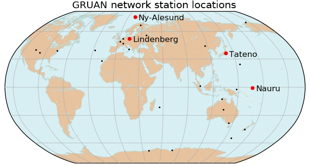
Figure 1Map of the GRUAN RS network. Labeled locations with red dots are RS stations used in this study, and black dots mark the other GRUAN network RS stations. For more information about these and other GRUAN stations, see https://www.gruan.org (last access: 25 April 2018).
All RS profiles are provided by the Global Climate Observing System (GCOS) Reference Upper-Air Network (GRUAN; see Bodeker et al., 2016, for more information on the GRUAN project) and downloaded from the National Oceanic and Atmospheric Administration (NOAA) National Climatic Data Center. GRUAN RS were chosen for their reference-quality observations and well-documented uncertainties (Seidel et al., 2009, 2011; Immler et al., 2010), allowing for a better analysis of the reduction of sampling errors associated with each co-location method.
We chose four stations in different climates for this study for the time periods of 2014, 2013, 2012, and 2011–2013, respectively: Lindenberg, Germany (LIN); Ny-Ålesund, Norway (NYA); Tateno, Japan (TAT); and Nauru, Nauru (NAU). (Nauru is the only station in which the full period of activation was used; this is due to the low number of RS launches during 2011 through late August 2013.) Figure 1 is a map of the GRUAN RS stations with the locations of the four stations used in this study labeled and marked in red. All four stations use the Vaisala RS92 radiosonde instruments (for details on GRUAN RS processing see Dirksen et al., 2014).
For refractivity comparisons, RS refractivity is computed under the assumption of a neutral atmosphere (Smith and Weintraub, 1953):
where N is refractivity (N−units), p is dry air pressure (hPa), T is temperature (Kelvin), and e is water vapor pressure (hPa).
We generate two data sets: an unfiltered data set which contains all original RO and RS profiles and a filtered data set containing the vertically filtered versions of the original RO and RS profiles.
2.2 Filtering
Representativeness errors result from two different aspects of the RO and RS observations. Firstly, GRUAN RS have a temporal resolution of 1 s, with vertical resolution of 5–10 m on average (Ladstädter et al., 2015), which is much finer than the 100 m vertical resolution of the RO wetPrf profiles. Secondly, RS observations are a series of point measurements, whereas RO observations are weighted averages of a cylindrical volume of atmosphere with horizontal scales of 150–300 km (Kursinski et al., 1997; Kuo et al., 2004; Anthes, 2011). Vertical filtering of both RO and RS profiles should decrease the representativeness errors caused by differences in observation type and vertical resolutions (Lohmann, 2007), resulting in a more meaningful comparison between profiles. Removal of structures with very small vertical scales also has the effect of reducing representativeness errors associated with different horizontal scales (footprints) of the observations (Kitchen, 1989). Structures with very small vertical scales in the RS profile are likely associated with horizontal scales too small to be resolved by the RO observations. Though the majority of previous RO–RS comparison studies do not filter the RO or RS profiles before comparison, Kuo et al. (2004) filtered the profiles to remove structures with vertical scales less than 1 km before comparison with model analyses in an effort to minimize vertical representativeness errors.
To remove small-scale, unrepresentative structures in both the RO and RS profiles, we applied the Savitzky–Golay low-pass filter (Savitzky and Golay, 1964). We first linearly interpolated profile variables (refractivity, temperature, and water vapor pressure) to a 10 hPa (∼ 100 m) uniform vertical grid, then filtered the full profile using a fixed 40 hPa (∼ 400 m) filter window and quadratic fitting polynomial. We tested various combinations of filter windows and number of passes to determine the effects of filtering on the RS and RO profiles (not shown). The number of passes of the same filter result in minor smoothing effects relative to different filter windows, and filter windows larger than 40 hPa cause too much smoothing of the RS profile. RO profiles, due to their lower resolution relative to the RS profiles, showed little change under different filter windows. Therefore, 40 hPa was chosen as a sufficient window to remove small-scale features in the RS profile while preserving the overall structures of both the RS and RO profiles. To accommodate for the differences in vertical resolution, RO profiles underwent a single pass of the 40 hPa filter and RS profiles underwent three passes of the 40 hPa filter.
2.3 RO–RS co-location criteria and statistics
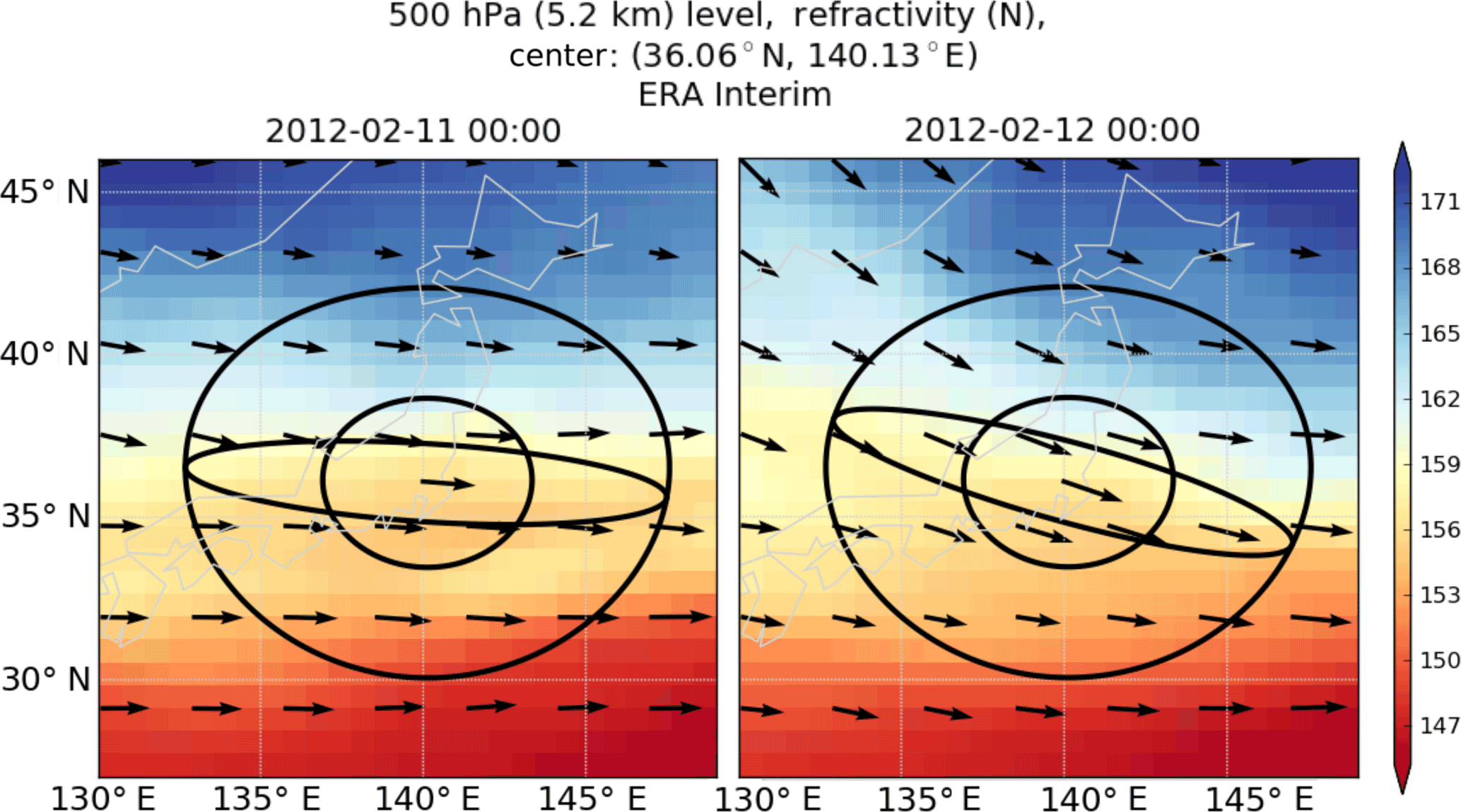
Figure 2500 hPa ERA-Interim refractivity field (color contours) centered at Tateno for 11 and 12 February 2012 at 00:00 UTC. The three spatial geometries (large circle, small circle, ellipse) are shown in black centered at Tateno with wind vectors (black) denoting wind direction and magnitude. Generally, refractivity isopleths lie parallel to the wind flow, even as wind direction changes, resulting in minimal refractivity variability within the ellipse relative to both circles.
We co-located RO and RS observations using the ellipse method every 10 hPa between 1000 and 10 hPa at each RS location. We included RO occultations taken within 3 h of the RS launch at Ny-Ålesund, Tateno, and Nauru and within 1 h at Lindenberg due to the high number of RS launches (at least four times daily). We considered three different geometric constraints to co-locate RO profiles: (1) large circle with 6∘ latitude radius (∼ 666 km); (2) small circle with 2.6∘ latitude radius (∼ 300 km); and (3) ellipse parallel to the wind direction, 6∘ latitude semi-major axis and 1.2∘ latitude (∼ 133 km) semi-minor axis, each centered at the RS location. (The ellipse and small circle are circumscribed by the large circle, and the small circle was chosen such that the area within the small circle and ellipse are approximately the same; see Fig. 2.) The X and Y coordinates of the points on the circles and ellipses are constructed using the following parameterization (a is semi-major axis, b is semi-minor axis; for circles, radius, where both a and b are in kilometers):
where s is a parameter that varies between 0 and 2π and is stepped in increments of 0.01, yielding a series of 629 points that approximate the circle or ellipse, and θ is the wind direction in radians (converted from meteorological to polar coordinates). The X and Y coordinates of the circle or ellipse are first computed at the Equator, where 1∘ of latitude and longitude equals 111 km, and then the X and Y coordinates are adjusted to the latitude and longitude of the RS station according to the following:
The ellipses change orientation such that the semi-major axis is parallel to the wind direction at each pressure level and time per RS. The circles remain fixed and unaffected by the change in wind direction, pressure level, or time.
Figure 2 illustrates the three geometries centered at Tateno at 500 hPa for 2 days in February 2012, noting that the ellipse adjusts its orientation as wind direction changes with time and at a pressure level. Preliminary testing of the ellipse co-location method with ERA-Interim model refractivity fields confirmed that refractivity isopleths tend to follow wind flow (as illustrated in Fig. 2); thus, orientation of the ellipse along the direction of the wind flow should increase atmospheric homogeneity relative to the large circle.
For each RS at a given time and pressure level, RO profiles are co-located with the RS profiles under the time and geometric constraints discussed above. There can be (and often are) multiple co-location pairs with the same RS at a given time and pressure level. We computed differences for each co-location pair:
where X refers to refractivity, temperature, or water vapor pressure. We computed the RMS of the differences for each pressure level over the full time period and used the RMS to quantify the reduction in sampling errors. In certain cases we also computed the percent difference between two quantities Xi and Xj:
2.4 Spatial–temporal sampling correction algorithm
Applying a spatial–temporal sampling correction to the RO–RS differences is an alternate method of reducing sampling errors in the presence of an auxiliary data set. This method has been applied in previous studies and is not restricted to RO–RS comparisons. Haimberger et al. (2012) used this approach to homogenize RS records. Wong et al. (2015) used ECMWF forecasts for double-differencing to reduce the sampling differences between Atmospheric Infrared Sounder (AIRS) and RS co-located pairs. Tradowsky et al. (2017) calculated an observed–background (O–B) double difference to estimate the mean RS temperature bias using co-located RO profiles and Met Office model background fields. These studies use a double-difference correction, but do not verify or discuss how the correction reduces sampling errors.
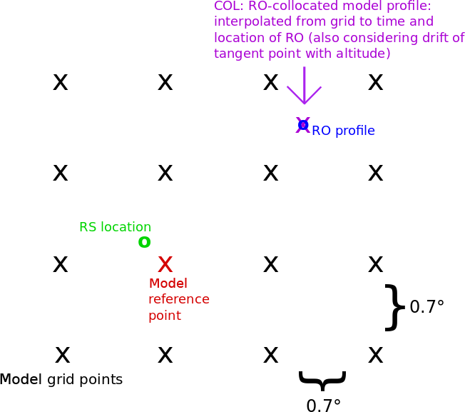
Here, we apply a spatial–temporal sampling correction double difference computed with model data and assess its effects on reducing sampling errors. We use ERA-Interim data to subtract the model background from both the RO and RS observations, removing spatial and temporal sampling differences and isolating the observational errors associated with the RO and RS pair. As shown in Fig. 3, we use the ERA-Interim profiles interpolated in time and space to the RO time and location (eraPrf files provided by CDAAC) and the ERA-Interim grid point nearest the RS location at the RS launch time to compute the sampling correction. Due to the coarser vertical resolution of the ERA-Interim grid relative to the RS and RO vertical resolutions, comparisons with the sampling correction are conducted on a common 50 hPa uniform pressure grid from 1000 to 100 hPa to avoid further vertical interpolation.
The spatial–temporal sampling corrected differences (Xsc) for the co-location pairs are computed as follows for the comparison variables (refractivity, temperature, and water vapor pressure):
where XERA(RO) is the ERA-Interim model value interpolated in time and space to the RO location, XERA(RS) is the ERA-Interim model grid point value closet to the RS at the RS launch time, and their difference, XERA(RO)−XERA(RS), is referred to as the model correction term. We computed the RMS differences per pressure level on the 50 hPa grid.
The spatial–temporal corrected difference (Xsc) between the two data sets (Eq. 6a and b) can be interpreted in two ways. When the two data sets are close to each other in time and space, one interpretation is that the RO–RS differences are corrected for local spatial and temporal variability by subtracting these sampling differences, which are estimated by another data set (in this case ERA-Interim) from the measured differences (Eq. 6b). This is the interpretation used here and by Wong et al. (2015). However, as the equivalent Eq. (6a) shows, the corrected difference is also the difference of the departures of the two data sets from a common, reference data set, or the “double-differencing” method (Chander et al., 2013; Tradowsky et al., 2017). In this interpretation, the two data sets are not necessarily required to be close in space or time; the method is valid as long as the biases of the reference data set do not vary over the spatial and temporal scales of the comparison. We tested the sensitivity of the sampling correction method to the spatial and temporal scale of the comparisons in Appendix A for RO–RS pairs over a much larger spatial scale (within circles of radius 15∘ latitude) and longer time window (24 h) at Lindenberg. We find that the RMS, mean, and standard deviations of the comparisons are insensitive over this range of spatial and temporal scales, allowing for a large increase in the number of co-located pairs of data.
Preliminary proof-of-concept testing of the ellipse method using only ERA-Interim data demonstrated a significant reduction in RMS refractivity differences within the ellipse relative to both the large circle and circles of similar area to the ellipse (not shown here). In the following two sections, aspects of the ellipse co-location are analyzed at the Lindenberg station. The final section presents the results of both the ellipse co-location and sampling correction at all four RS stations.
3.1 Filtered vs. unfiltered
Table 1Filtered vs. unfiltered RMS percent differences* for refractivity, temperature, and water vapor pressure at Lindenberg, 2014. RMS differences are computed using all co-located pairs within 100 hPa pressure layers for the filtered and unfiltered data sets, and then the percent differences between the two are computed and reported here.
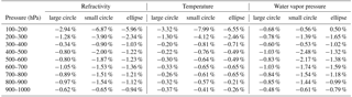
* Percent differences computed as 100 × (RMSfilt – RMSunfilt)∕RMSunfilt.
Filtering both the RO and RS profiles has a small, positive impact on reducing RMS differences in refractivity, temperature, and water vapor pressure. Compared to RMS differences computed using the unfiltered profiles at Lindenberg, filtering both the RO and RS profiles before co-location reduces RMS differences by about 1 % on average, up to almost 8 % in some instances (see Table 1). Within the large circle, filtering has less of an impact on reducing vertical representativeness percent errors since sampling errors tend to dominate (mostly due to large spatial differences). The RO–RS percent differences in the small circle and ellipse are more affected by vertical representativeness errors since the sampling errors are relatively small. Based on these results, we filtered all RO and RS profiles before computing their differences to reduce representativeness errors.
3.2 Effects of wind speed on ellipse co-location
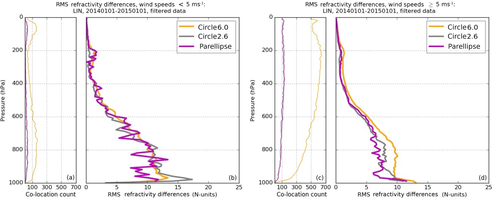
Figure 4RMS refractivity differences at Lindenberg 2014 for two sets of RO–RS pairs separated by reported RS wind speeds: pairs with wind speeds less than 5 m s−1 (a, b) and pairs with wind speeds greater than or equal to 5 m s−1 (c, d). Geometric constraints are shown in the following colors: large circle (orange), small circle (grey), and ellipse (magenta).
The relationship between the wind direction and horizontal variability (and sampling error) of refractivity is expected to break down for light wind speeds – indeed we found that when wind speeds are low, the effectiveness of orienting the ellipse along the direction of wind flow is significantly reduced. We separated co-located RO–RS pairs at Lindenberg into two groups based on the reported wind speed of the RS at a given time and pressure level: (1) wind speeds less than 5 m s−1 and (2) wind speeds greater than or equal to 5 m s−1. Figure 4 shows the RMS differences in refractivity for each group.
As shown in Fig. 4, the clear distinction between RMS profiles for the ellipse and two circles at wind speeds greater than 5 m s−1 essentially vanishes when wind speeds are less than 5 m s−1. Similarities in RMS refractivity differences when wind speeds are less than 5 m s−1 are likely associated with greater atmospheric homogeneity and weaker gradients in the region, resulting in similar observations within the area containing both circles and the ellipse. When wind speeds increase to larger than 5 m s−1, there is a greater separation between the circles and ellipse with respect to the RMS difference. Under moderate to high wind speed conditions, the ellipse reduces RMS refractivity differences relative to both the large and small circle, particularly below about 700 hPa. In the upper troposphere, both the ellipse and the smaller circle give similar results and smaller RMS differences than the large circle (Fig. 4). In the case of Lindenberg, since the majority of wind speeds are greater than 5 m s−1 (as noted by the differences in co-location counts under the two wind constraints in Fig. 4), low wind speeds do not have a significant effect on the overall RMS differences when co-location pairs are not separated by wind speed (see Fig. 5).
3.3 Ellipse co-location and sampling correction applied at four RS stations

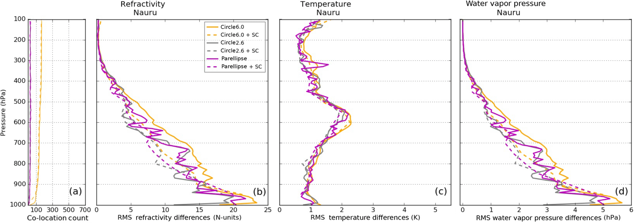
Figure 5RMS differences for RO–RS co-locations at Lindenberg, 2014. RMS differences with ellipse method only (solid; large circle: orange; small circle: grey; ellipse: magenta) and RMS differences with ellipse method and sampling correction (dashed, abbreviated as SC) are shown for all three variables: (b) refractivity, (c) temperature, and (d) water vapor pressure. The number of pairs within each ellipse (solid) and ellipse plus sampling correction (dashed) is shown in panel (a).

Figure 6Same as Fig. 5 for two different locations: Ny-Ålesund, 2013 (a–d) and Tateno, 2012 (e–h).
We carried out two RO–RS comparisons at four different RS locations (Lindenberg, Ny-Ålesund, Tateno, and Nauru): first, we compared pairs with RO observations co-located within the large circle, small circle, and ellipse centered at the RS station, and second, we applied the sampling correction to the RO–RS pairs within the ellipse and two circles. We then computed RMS differences in refractivity, temperature, and water vapor pressure.
Figure 5 illustrates the RMS differences for refractivity, temperature, and water vapor pressure with and without the sampling correction at Lindenberg. Considering the ellipse method only (solid lines), the ellipse reduces RMS differences relative to the large circle for all three variables at all pressure levels, having the most significant reduction in the temperature RMS differences. Generally, the small circle and ellipse have similar RMS differences, but there are pressure layers in which the ellipse reduces the RMS relative to the small circle. When the sampling correction is applied to the circles and ellipse (dashed lines), the RMS differences are significantly reduced and converge with minimal differences between the ellipse and circles. The RMS differences at Lindenberg are mostly affected by spatial sampling errors; temporal sampling errors are minimized by the reduced time window of 1 h due to frequent (four times daily) RS launches at this station.
The results at Ny-Ålesund and Tateno are very similar to those at Lindenberg, with some minor differences in the lower troposphere (Fig. 6). Again, using pairs in the ellipse only (solid, magenta) results in significantly reduced RMS differences relative to the large circle (solid, orange) and equal to or smaller RMS differences compared to the small circle (solid, grey). Including the sampling correction shows the largest reduction in RMS differences such that the differences from all three geometric types converge to similar values. At both Ny-Ålesund and Tateno, the reduction of RMS differences in the ellipse compared to the large circle becomes less in the lower troposphere (below 800 hPa), where the frequency of wind speeds less than 5 m s−1 increases and the relationship between wind direction and RO–RS differences breaks down. For example, at Ny-Ålesund and Tateno the percentages of RO–RS pairs for which the wind speed is less than 5 m s−1 below 800 hPa are 36.1 and 32.7 %, respectively. The small sample size in the ellipse compared to the large circle (Fig. 6a, e) may also play a role, allowing a few outliers to dominate the statistics.
The results at the tropical location of Nauru (Fig. 7) generally confirm the findings at the other three RS locations. The ellipse alone (solid, magenta) decreases RMS differences relative to the large circle (solid, orange) and produces RMS differences that are comparable to the differences of the small circle (solid, grey). There is less distinction, however, between the ellipse method only (solid) and sampling correction (dashed) RMS differences, particularly for temperature. All six geometric and sampling correction combinations have overlapping RMS temperature differences and show little separation between co-location methods, unlike the results at Lindenberg, Ny-Ålesund, and Tateno. This is most likely caused by the relative horizontal homogeneity in temperature at Nauru, which is located in the deep tropics. Thus, there is little to no distinction between RMS temperature differences using various geometrical constraints or sampling correction.
Refractivity and water vapor pressure RMS differences in the lower troposphere (1000–700 hPa) at Nauru are the largest of the four stations, caused primarily by atmospheric conditions at its location in the deep tropics. RO is known to have negative refractivity biases in the lower troposphere, particularly in moist tropical regions where large water vapor and associated refractivity gradients often result in super-refraction (Rocken et al., 1997; Ao et al., 2003; Sokolovskiy, 2003; Beyerle et al., 2006; Anthes et al., 2008). Overall, this results in larger RMS refractivity differences at Nauru. Since super-refraction is an error characteristic of RO retrievals and not related to horizontal sampling errors, the sampling correction has no impact on the RO–RS refractivity differences.
We have shown that vertical filtering of the RO and RS profiles before comparison reduces representativeness errors associated with different vertical resolutions and observation types by a small amount (typically a few percent). Using these filtered profiles, we tested two methods to reduce spatial and temporal sampling errors during RO–RS comparisons: (1) restricting RO and RS pairs to within ellipses oriented along the direction of wind flow and (2) applying a spatial–temporal sampling correction using model data to remove differences caused by horizontal atmospheric gradients and time differences in the observations. When wind speeds exceed about 5 m s−1, co-locations within the ellipse parallel to the wind flow reduce RMS differences in refractivity, temperature, and water vapor pressure relative to co-locations within the large circle and either reduce or result in RMS differences that are approximately equal to the differences within the smaller circle. The effectiveness of co-locating RO–RS pairs within the ellipse is reduced for wind speeds less than 5 m s−1.
Applying the spatial–temporal sampling correction using ERA-Interim model data showed the most significant reduction in RMS differences, more so than applying the ellipse constraint alone. The sampling correction reduced RMS differences in refractivity, temperature, and water vapor pressure by an average of 55 %. The reductions of sampling errors within both large and small circles and the ellipse tend to converge with the sampling correction applied, rendering the differences in geometric constraints of the circles and ellipse negligible. An exception to this reduction in RMS occurs at Nauru in the lower troposphere, where super-refraction associated with the atmospheric conditions of the deep tropics tends to dominate the RMS differences.
In order to reduce sampling errors for future RO–RS co-location comparisons, our results suggest that applying the sampling correction under more lenient co-location criteria would be most effective. By using a large distance constraint, the sample size will be sufficiently large and applying the sampling correction eliminates most sampling errors, even for the large distance restriction (greater than 600 km). However, if a reliable model is unavailable, restricting co-locations within ellipses oriented along the direction of wind flow will help to reduce sampling errors caused by atmospheric variability. Both of these methods are effective in reducing sampling errors caused by spatial and temporal differences during comparisons and should provide a more accurate error analysis of RO and RS observations.
The code used in this study will be made available upon request.
A1 Mean and standard deviation of differences
In this section, we compute the mean and standard deviation (SD) of the RO–RS differences. The mean difference is defined as
The variance about the mean is given by
and the standard deviation of the difference about the mean is the square root of the variance, SDM = VAR. The SDM can be compared to the RMS RO–RS difference, which is defined by
where the mean square difference (MS) is defined as
It can be shown by expanding Eq. (A2) that
Thus, the SDM(RO−RS) is always less than or equal to the RMS(RO−RS), and equal if and only if the mean RO–RS difference is zero.
Figures A1–A3 show the mean and SD of the RO–RS differences for refractivity, temperature, and water vapor pressure, respectively, for all six co-location methods. For each variable, the mean difference profiles are all similar and show no systematic differences, which indicates that the mean differences are not sensitive to the co-location method and are relatively unaffected by sampling errors. This is because the distribution of the RO observations with respect to the RS observations is approximately random, and so the sampling (and representativeness) errors tend to cancel for a large enough sample size. However, the mean differences do illustrate differences in bias errors between the two data sets. The bias errors in the GRUAN RS are expected to be small, so the differences in the mean RO–RS differences are likely due to the RO biases, notably the negative refractivity bias caused by super-refraction in the lower troposphere under moist conditions.
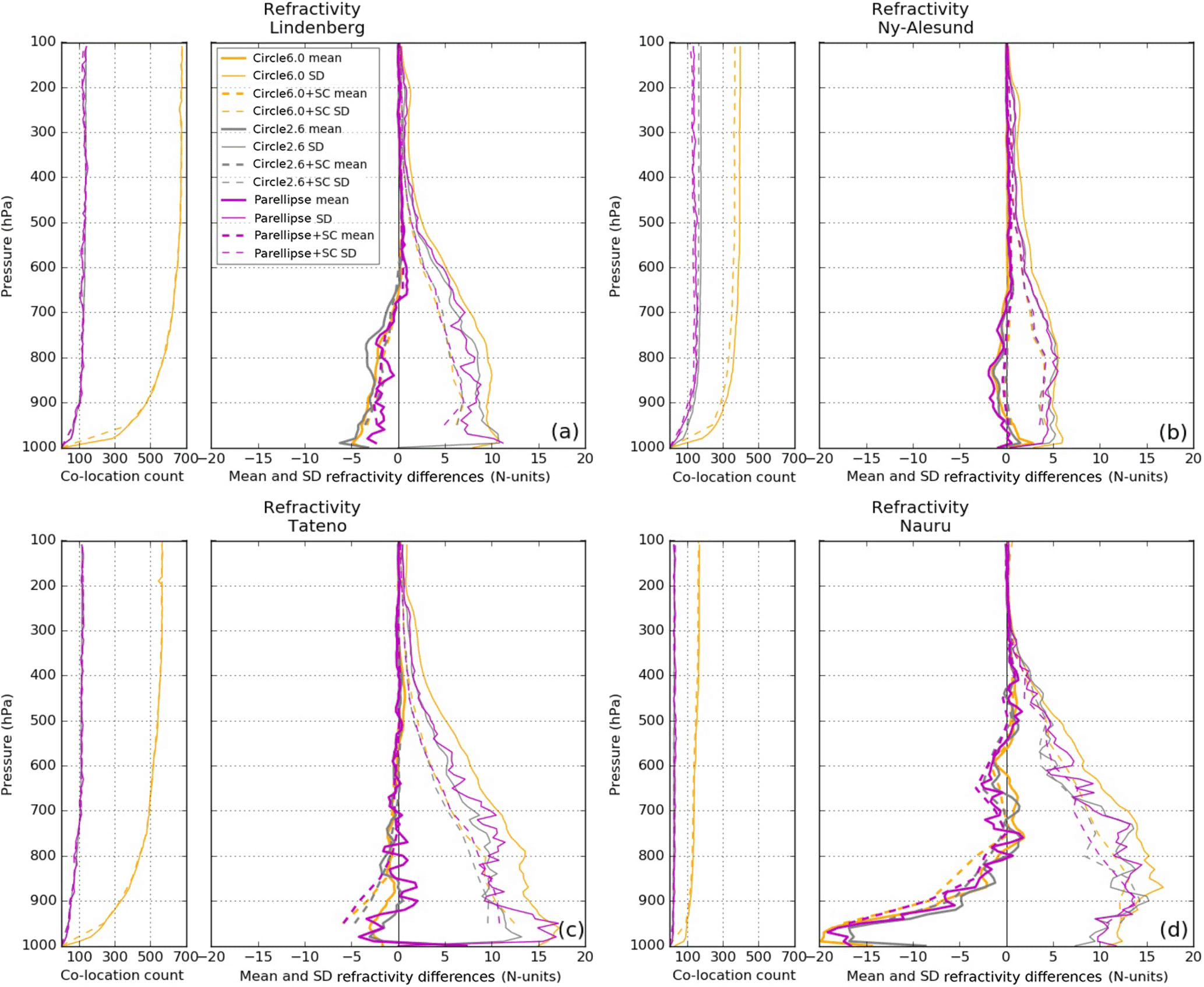
Figure A1RO–RS refractivity mean (thick) and SD (thin) difference profiles for the six co-location methods at Lindenberg (a), Ny-Ålesund (b), Tateno (c), and Nauru (d). The number of co-located RO–RS pairs are given on the left side of each panel (without the sampling correction: solid; with the sampling correction: dashed). The color schemes are the same as Figs. 4–7 and are given in the legend in (a) where SC stands for sampling correction.
In Fig. A1 we see that the differences in mean refractivity are small above 700 hPa for all four stations. Below 700 hPa, there is a negative RO refractivity bias, which is most pronounced at the tropical Nauru station where super-refraction is most common. The bias is minimal at the most northern station, Ny-Ålesund, which is expected to have the fewest cases of super-refraction.
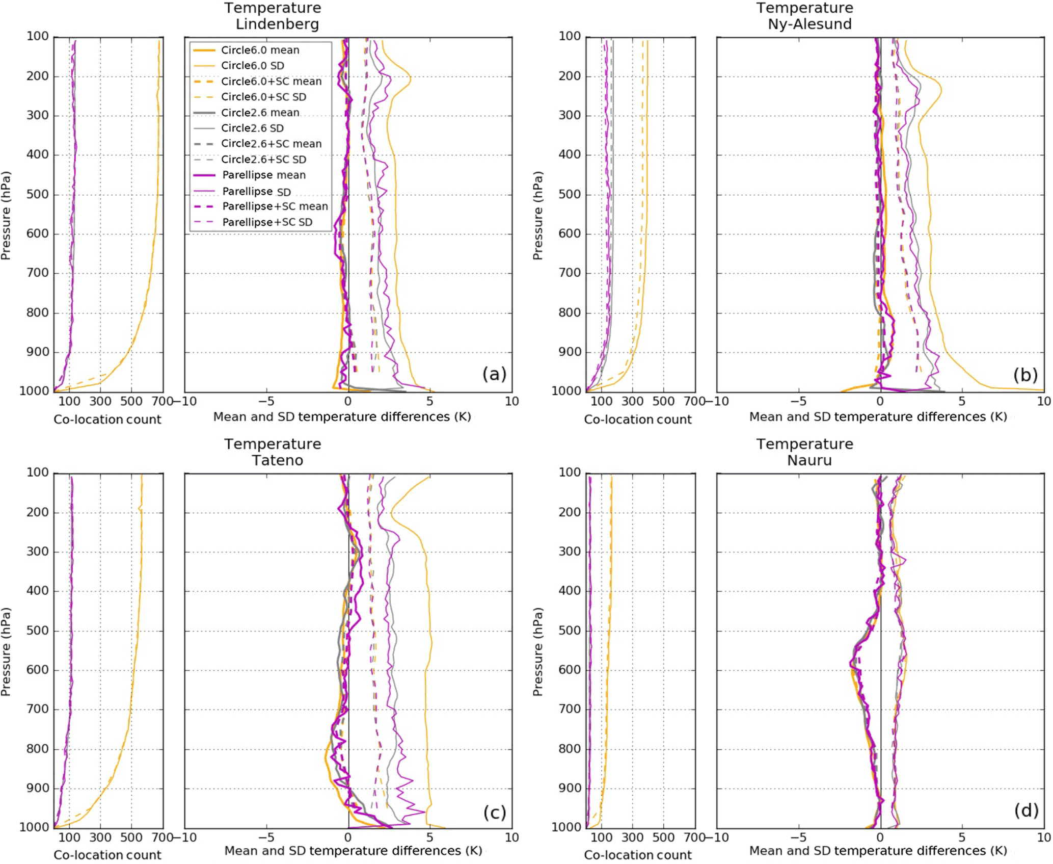
The biases for temperature differences (Fig. A2) are less than 1 K from 1000 to 100 hPa for Lindenberg, Ny-Ålesund, and Tateno and show a negative bias at Nauru, reaching about 2 K at 600 hPa. This is probably not caused by super-refraction in the RO observations because the negative bias is above the level where most super-refraction occurs and the bias becomes smaller below the 600 hPa level, in contrast to the bias in refractivity, which increases sharply with decreasing height in the lower troposphere. Instead, the bias in the temperature is probably related to the 1D-VAR retrieval of temperature in the RO observation, which uses ERA-Interim temperatures as the first guess.
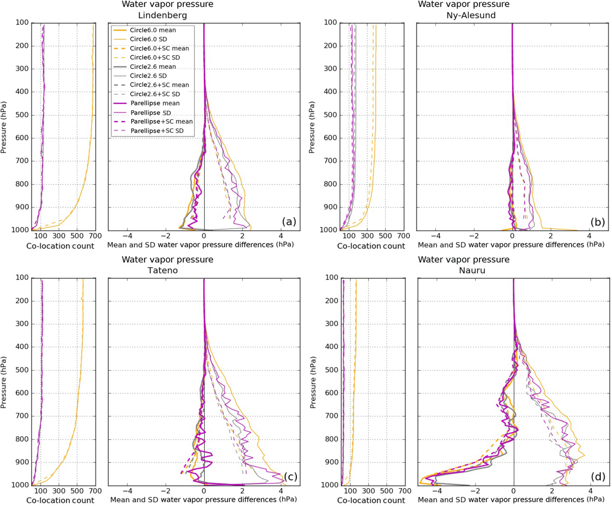
Finally, the differences in the mean RO–RS water vapor pressure reflect the negative refractivity bias due to super-refraction at Lindenberg, Tateno, and especially Nauru, with little bias at the colder, drier Ny-Ålesund station (Fig. A3).
The SD profiles in Figs. A1–A3 are similar to the RMS profiles associated with the different co-location methods in Figs. 5–7. This is expected because the SD and RMS values are close when mean RO–RS differences are near zero, as shown by Eq. (A5). The largest differences between the SD and RMS profiles are in the lower troposphere, where the mean differences are the largest.
A2 Sensitivity of spatial–temporal correction method to spatial and temporal scale
In Sect. 2.4, we noted that when using the double-differencing correction method to reduce spatial and temporal sampling errors, it was not necessary that the RO profiles be close in space and time to the RS profiles, as long as the biases of the reference data set (in our case ERA-Interim) remain constant in space and time throughout the comparison. To illustrate this property of the double-differencing method, we co-located RO profiles within a much larger circle (15∘ latitude radius, ∼ 1665 km) and a time window of 24 h at Lindenberg between January and March 2014 and compared the RMS, mean, and SD of these RO–RS differences to those computed under the 6 and 2.6∘ radius circles with a 1 h time window.
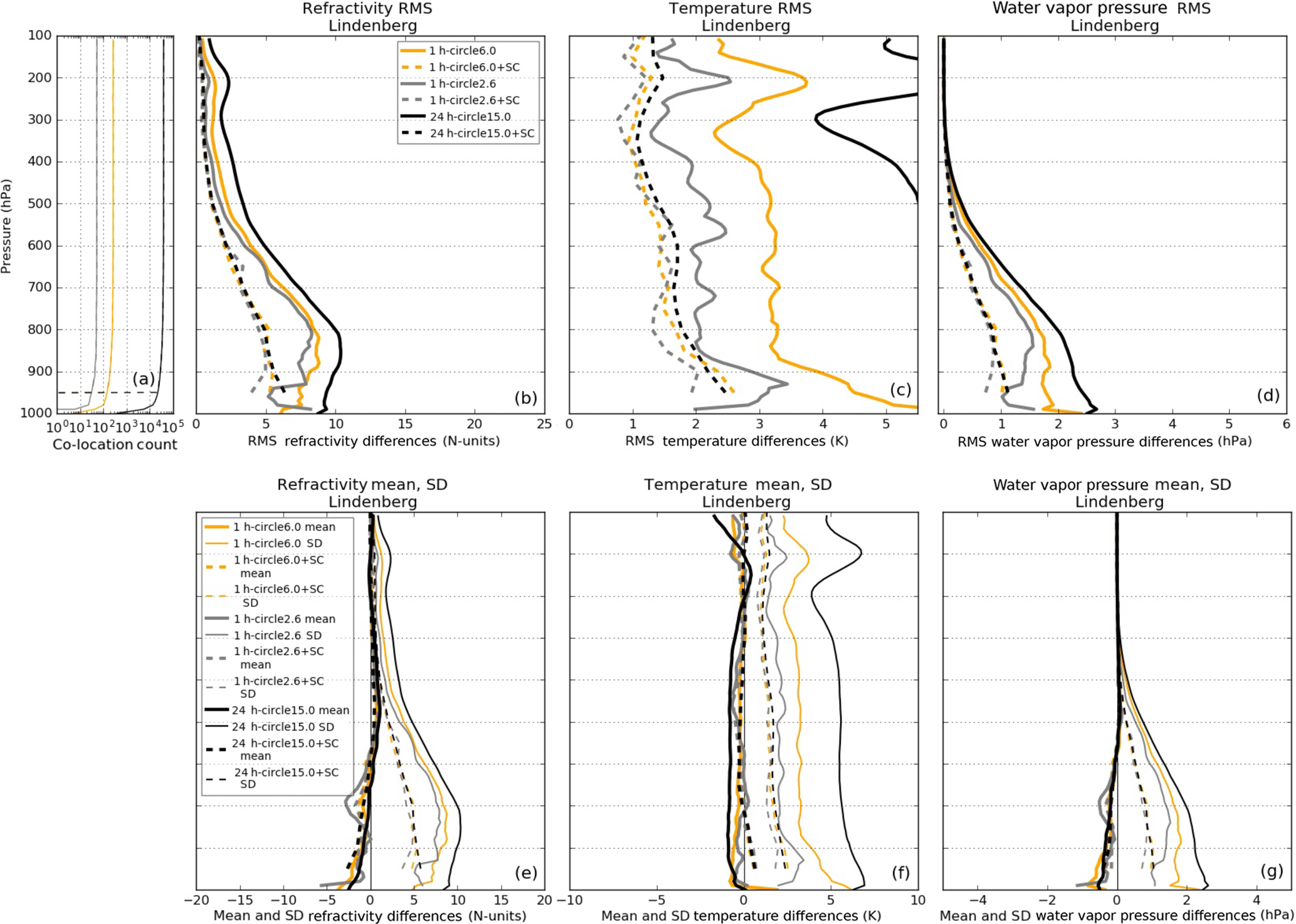
Figure A4RMS (b–d), mean (thick; e–g), and SD (thin; e–g) RO–RS profiles for refractivity (b, e), temperature (c, f), and water vapor pressure (d, g) under three different co-location restraints with (dashed) and without (solid) the sampling correction (SC) applied: circles of radius 6∘ latitude (orange) and 2.6∘ latitude (grey) for time windows of 1 h, and a circle of radius 15∘ latitude for a 24 h time window (black). Comparisons are conducted at Lindenberg for January–March 2014. The number of co-located pairs for each co-location restraint (with SC: dashed; without SC: solid) are given in panel (a), where the x axis is a logarithm scale.
Figure A4 illustrates the RMS (b–d), mean, and SD (e–g) profiles for the RO–RS differences in refractivity, temperature, and water vapor pressure under the three different co-location restraints with and without the sampling correction applied. Across all three variables, the RMS, mean, and SD profiles with the sampling correction remain nearly the same regardless of the spatial or temporal differences applied to the RO–RS co-location. This verifies that the double-differencing method is insensitive to spatial and temporal separations of the RO and RS observations for this example when using ERA-Interim as a reference data set. The similarity in the RMS, mean, and SD profiles with the sampling correction also indicates that any existing bias in the ERA-Interim reference data set is nearly constant over these spatial and temporal scales.
These results show that using the double-differencing method to reduce spatial and temporal sampling errors in RO–RS comparisons allows for many more RO–RS pairs to be included in the comparison (more than 35 000 for the 15∘ circle with 24 h time window compared to approximately 250 for the 6∘ circle and 1 h time window), as illustrated Fig. A4a, provided that the bias of the reference data set does not vary significantly over the spatial and temporal scales of the comparison. Increasing the size of the spatial and temporal scales of the comparison is thus a tradeoff between reducing the random error effects by increasing sampling size and possibly increasing the errors by allowing a greater effect of varying biases in the reference data set.
All co-authors contributed to developing the ideas and methodologies of this project. SG conducted the majority of the coding, data retrieval, computations, and analysis, with TR contributing to coding and data retrieval. SG prepared the manuscript with contributions from both co-authors.
The authors declare that they have no conflict of interest.
The authors thank Eric DeWeaver (NSF) and Jack Kaye (NASA) for their
support of this research through NSF-NASA grant AGS-1522830. Sergey Sokolovskiy provided many useful comments and suggestions during this study.
The first author was supported in part by the Significant Opportunities in
Atmospheric Research and Science (SOARS) program, NSF grant AGS-1641177, and
by the Constellation Observing System for Meteorology, Ionosphere, and
Climate (COSMIC) program at UCAR, which is sponsored by the National Space
Office in Taiwan, NSF, NASA, NOAA, and the U.S. Air Force. Thanks to CDAAC
for the provided RO data sets, NOAA NCDC and GRUAN for the provided RS data
sets, and the ECMWF for the provided ERA-Interim data sets. The authors thank
Keith Maull for his suggestions during this study. The authors would like
to thank the three anonymous reviewers for their comments and constructive
suggestions which improved this paper.
Edited by: Marcos Portabella
Reviewed by: three anonymous referees
Anthes, R., Bernhardt, P., Chen, Y., Cucurull, L., Dymond, K., Ector, D., Healy, S., Ho, S.-P., Hunt, D., Kuo, Y.-H., Liu, H., Manning, K., McCormick, C., Meehan, T., Randel, W., Rocken, C., Schreiner, W., Sokolovskiy, S., Syndergaard, S., Thompson, D. C., Trenberth, K., Wee, T.-K., Yen, N., and Zeng, Z.: The COSMIC/FORMOSAT-3 Mission-Early Results, B. Am. Meteorol. Soc., 89, 313–333, https://doi.org/10.1175/BAMS-89-3-313, 2008. a
Anthes, R. A.: Exploring Earth's atmosphere with radio occultation: contributions to weather, climate and space weather, Atmos. Meas. Tech., 4, 1077–1103, https://doi.org/10.5194/amt-4-1077-2011, 2011. a
Ao, C., Meehan, T., Hajj, G., Mannucci, A., and Beyerle, G.: Lower troposphere refractivity bias in GPS occultation retrievals, J. Geophys. Res., 108, 4577, https://doi.org/10.1029/2002JD003216, 2003. a
Beyerle, G., Schmidt, T., Wickert, J., Heise, S., Rothacher, M., Konig-Langlo, G., and Lauristen, K.: Observations and simulations of receiver-induced refractivity biases in GPS radio occultation, J. Geophys. Res., 111, D12101, https://doi.org/10.1029/2005JD006673, 2006. a
Bodeker, G., Bojinski, S., Cimini, D., Dirksen, R., Haeffelin, M., Hannigan, J., Hurst, D., Leblanc, T., Madonna, F., Maturilli, M., Mikalsen, A., Philipona, R., Reale, T., Seidel, D., Tan, D., Thorne, P., Vömel, H., and Wang, J.: Reference upper-air observations for climate: from concept to realty, B. Am. Meteorol. Soc., 97, 123–135, https://doi.org/10.1175/BAMS-D-14-00072.1, 2016. a
Bruce, R., Duncan, L., and Pierluissi, J.: Experimental study of the relationship between radiosonde temperatures and satellite-derived temperatures, Mon. Weather Rev., 105, 493–496, 1977. a
Chander, G., Hewison, T., Fox, N., Wu, X., Xiong, X., and Blackwell, W.: Overview of intercalibration of satellite instruments, IEEE T. Geosci. Remote, 15, 1056–1080, https://doi.org/10.1109/TGRS.2012.2228654, 2013. a, b
Dee, D. P., Uppala, S. M., Simmons, A. J., Berrisford, P., Poli, P., Kobayashi, S., Andrae, U., Balmaseda, M. A., Balsamo, G., Bauer, P., Bechtold, P., Beljaars, A. C. M., van de Berg, L., Bidlot, J., Bormann, N., Delsol, C., Dragani, R., Fuentes, M., Geer, A. J., Haimberger, L., Healy, S. B., Hersbach, H., Holm, E. V., Isaksen, L., Kallberg, P., Koehler, M., Matricardi, M., McNally, A. P., Monge-Sanz, B. M., Morcrette, J. J., Park, B. K., Peubey, C., de Rosnay, P., Tavolato, C., Thepaut, J. N., and Vitart, F.: The ERA-Interim reanalysis: configuration and performance of the data assimilation system, Q. J. Roy. Meteor. Soc., 137, 553–597, https://doi.org/10.1002/qj.828, 2011. a
Dirksen, R. J., Sommer, M., Immler, F. J., Hurst, D. F., Kivi, R., and Vömel, H.: Reference quality upper-air measurements: GRUAN data processing for the Vaisala RS92 radiosonde, Atmos. Meas. Tech., 7, 4463–4490, https://doi.org/10.5194/amt-7-4463-2014, 2014. a
Eyre, J.: Assimilation of radio occultation measurements into a numerical weather prediction system, Technical Memorandum 199, European Centre for Medium-Range Weather Forecasts, Reading, UK, 1994. a
Fassò, A., Ignaccolo, R., Madonna, F., Demoz, B. B., and Franco-Villoria, M.: Statistical modelling of collocation uncertainty in atmospheric thermodynamic profiles, Atmos. Meas. Tech., 7, 1803–1816, https://doi.org/10.5194/amt-7-1803-2014, 2014. a
Haimberger, L., Tavolato, C., and Sperka, S.: Homogenization of the global radiosonde temperature dataset through combined comparison with reanalysis background series and neighboring stations, J. Climate, 25, 8108–8131, https://doi.org/10.1175/JCLI-D-11-00668.1, 2012. a
He, W., Ho, S.-P., Chen, H., Zhou, X., Hunt, D., and Kuo, Y.-H.: Assessment of radiosonde temperature measurements in the upper troposphere and lower stratosphere using COSMIC radio occultation data, Geophys. Res. Lett., 36, L17807, https://doi.org/10.1029/2009GL038712, 2009. a
Ho, S.-P., Zhou, X., Kuo, Y.-H., Hunt, D., and Wang, J.: Global evaluation of radiosonde water vapor systematic biases using GPS radio occultation from COSMIC and ECMWF analysis, Remote Sensing, 2, 1320–1330, https://doi.org/10.3390/rs2051320, 2010. a
Ignaccolo, R., Fraco-Villoria, M., and Fasso, A.: Modelling collocation uncertainty of 3D atmospheric profiles, Stoch. Env. Res. Risk A., 29, 417–429, https://doi.org/10.1007/s00477-014-0890-7, 2015. a
Immler, F. J., Dykema, J., Gardiner, T., Whiteman, D. N., Thorne, P. W., and Vömel, H.: Reference Quality Upper-Air Measurements: guidance for developing GRUAN data products, Atmos. Meas. Tech., 3, 1217–1231, https://doi.org/10.5194/amt-3-1217-2010, 2010. a
Kitchen, M.: Representativeness errors for radiosonde observations, Q. J. Roy. Meteor. Soc., 115, 673–700, 1989. a, b
Kuo, Y.-H., Wee, T., Sokolovskiy, S., Rocken, C., Schreiner, W., Hunt, D., and Anthes, R.: Inversion and error estimation of GPS radio occultation data, J. Meteorol. Soc. Jpn., 82, 507–531, https://doi.org/10.2151/jmsj.2004.507, 2004. a, b
Kuo, Y.-H., Schreiner, W., Wang, J., Rossiter, D., and Zhang, Y.: Comparison of GPS radio occultation soundings with radiosondes, Geophys. Res. Lett., 32, L05817, https://doi.org/10.1029/2004GL021443, 2005. a, b
Kursinski, E., Hajj, G., Schofield, J., Linfield, R., and Hardy, K.: Observing Earth's atmosphere with radio occultation measurements using the Global Positioning System, J. Geophys. Res., 102, 23429–23465, https://doi.org/10.1029/97JD01569, 1997. a
Ladstädter, F., Steiner, A. K., Schwärz, M., and Kirchengast, G.: Climate intercomparison of GPS radio occultation, RS90/92 radiosondes and GRUAN from 2002 to 2013, Atmos. Meas. Tech., 8, 1819–1834, https://doi.org/10.5194/amt-8-1819-2015, 2015. a
Lohmann, M.: Analysis of Global Positioning System (GPS) radio occultation measurement errors based on Satellite de Aplicaciones Cientificas-C (SAC-C) GPS radio occultation data recorded in open-loop and phase-locked-loop mode, J. Geophys. Res., 112, D09115, https://doi.org/10.1029/2006JD007764, 2007. a
Mears, C., Wang, J., Smith, D., and Wentz, F.: Intercomparison of total precipitable water measurements made by satellite-borne microwave radiometers and ground-based GPS instruments, J. Geophys. Res., 120, 2492–2504, https://doi.org/10.1002/2014JD022694, 2015. a
Melbourne, W., Davis, E., Duncan, C., Hajj, G., Hardy, K., Kursinski, E., Meehan, T., Young, L., and Yunck, T.: The application of space borne GPS to atmospheric limb sounding and global change monitoring, Tech. rep., Jet Propulsion Lab., California Institute of Technology, 1994. a
Rocken, C., Anthes, R. A., Exner, M., Hunt, D., Sokolovskiy, S., Ware, R., Gorbunov, M., Schreiner, W., Feng, D., Herman, B., Kuo, Y.-H., and Zou, X.: Analysis and validation of GPS/MET data in the neutral atmosphere, J. Geophys. Res., 102, 29849–29866, https://doi.org/10.1029/97JD02400, 1997. a
Savitzky, A. and Golay, M.: Smoothing and differentiation of data by simplified least squares procedure, Anal. Chem., 36, 1627–1639, 1964. a
Seidel, D., Sun, B., Pettey, M., and Reale, A.: Global radiosonde balloon drift statistics, J. Geophys. Res., 116, D07102, https://doi.org/10.1029/2010JD014891, 2011. a
Seidel, D. J., Berger, F. H., Diamond, H. J., Dykema, J., Goodrich, D., Immler, F., Murray, W., Peterson, T., Sisterson, D., Sommer, M., Thorne, P., Voemel, H., and Wang, J.: Reference upper-air observations for climate Rationale, Progress, and Plans, B. Am. Meteorol. Soc., 90, 361–369, https://doi.org/10.1175/2008BAMS2540.1, 2009. a
Smith, E. K. and Weintraub, S.: The constants in the equation for atmospheric refractive index at radio frequencies, P. IRE, 41, 1035–1037, 1953. a
Sokolovskiy, S.: Effect of superrefraction on inversions of radio occultation signals in the lower troposphere, Radio Sci., 38, 1058, https://doi.org/10.1029/2002RS002728, 2003. a
Staten, P. and Reichler, T.: Apparent precision of GPS radio occultation temperatures, Geophys. Res. Lett., 36, L24806, https://doi.org/10.1029/2009GL041046, 2009. a
Sun, B., Reale, A., Seidel, D. J., and Hunt, D. C.: Comparing radiosonde and COSMIC atmospheric profile data to quantify differences among radiosonde types and the effects of imperfect collocation on comparison statistics, J. Geophys. Res., 115, D23104, https://doi.org/10.1029/2010JD014457, 2010. a, b
Tradowsky, J., Burrows, C., Healy, S., and Eyre, J.: A new method to correct radiosonde temperature biases using radio occultation data, J. Appl. Meteorol. Clim., 56, 1643–1661, https://doi.org/10.1175/JAMC-D-16-0136.1, 2017. a, b, c
Vergados, P., Mannucci, A., and Ao, C.: Assessing the performance of GPS radio occultation measurements in retrieving tropospheric humidity in cloudiness: A comparison study with radiosondes, ERA-Interim, and AIRS data sets, J. Geophys. Res., 19, 7718–7731, https://doi.org/10.1002/2013JD021398, 2014. a
Wang, B.-R., Liu, X.-Y., and Wang, J.-K.: Assessment of COSMIC radio occultation retrieval product using global radiosonde data, Atmos. Meas. Tech., 6, 1073–1083, https://doi.org/10.5194/amt-6-1073-2013, 2013. a
Ware, R., Exner, M., Feng, D., Gorbunov, M., Hardy, K., Herman, B., Kuo, Y.-H., Meehan, T., Melbourne, W., Rocken, C., Schreiner, W., Sokolovskiy, S., Solheim, F., Zou, X., Anthes, R. A., Businger, S., and Trenberth, K.: GPS sounding of the atmosphere from low earth orbit: Preliminary results, B. Am. Meteorol. Soc., 77, 19–40, https://doi.org/10.1175/1520-0477(1996)077<0019:GSOTAF>2.0.CO;2, 1996. a
Wickert, J., Schmidt, T., Beyerle, G., Konig, R., and Reigber, C.: The radio occultation experiment aboard CHAMP: Operational data analysis and validation of vertical atmospheric profiles, J. Meteorol. Soc. Jpn., 82, 381–395, https://doi.org/10.2151/jmsj.2004.381, 2004. a
Wong, S., Fetzer, E., Schreier, M., Manipon, G., Fishbein, E., Kahn, B., Yue, Q., and Irion, F.: Cloud-induced uncertainties in AIRS and ECMWF temperature and specific humidity, J. Geophys. Res., 120, 1880–1901, https://doi.org/10.1002/2014JD022440, 2015. a, b
Xu, X., Luo, J., and Shi, C.: Comparison of COSMIC radio occultation refractivity profiles with radiosonde measurements, Adv. Atmos. Sci., 26, 1137–1145, https://doi.org/10.1007/s00376-009-8066-y, 2009. a
Zhang, K., Fu, E., Silcock, D., Wang, Y., and Kuleshov, Y.: An investigation of atmospheric temperature profiles in the Australian region using collocated GPS radio occultation and radiosonde data, Atmos. Meas. Tech., 4, 2087–2092, https://doi.org/10.5194/amt-4-2087-2011, 2011. a