the Creative Commons Attribution 3.0 License.
the Creative Commons Attribution 3.0 License.
Integrating uncertainty propagation in GNSS radio occultation retrieval: from excess phase to atmospheric bending angle profiles
Gottfried Kirchengast
Marc Schwaerz
Global Navigation Satellite System (GNSS) radio occultation (RO) observations are highly accurate, long-term stable data sets and are globally available as a continuous record from 2001. Essential climate variables for the thermodynamic state of the free atmosphere – such as pressure, temperature, and tropospheric water vapor profiles (involving background information) – can be derived from these records, which therefore have the potential to serve as climate benchmark data. However, to exploit this potential, atmospheric profile retrievals need to be very accurate and the remaining uncertainties quantified and traced throughout the retrieval chain from raw observations to essential climate variables. The new Reference Occultation Processing System (rOPS) at the Wegener Center aims to deliver such an accurate RO retrieval chain with integrated uncertainty propagation. Here we introduce and demonstrate the algorithms implemented in the rOPS for uncertainty propagation from excess phase to atmospheric bending angle profiles, for estimated systematic and random uncertainties, including vertical error correlations and resolution estimates. We estimated systematic uncertainty profiles with the same operators as used for the basic state profiles retrieval. The random uncertainty is traced through covariance propagation and validated using Monte Carlo ensemble methods. The algorithm performance is demonstrated using test day ensembles of simulated data as well as real RO event data from the satellite missions CHAllenging Minisatellite Payload (CHAMP); Constellation Observing System for Meteorology, Ionosphere, and Climate (COSMIC); and Meteorological Operational Satellite A (MetOp). The results of the Monte Carlo validation show that our covariance propagation delivers correct uncertainty quantification from excess phase to bending angle profiles. The results from the real RO event ensembles demonstrate that the new uncertainty estimation chain performs robustly. Together with the other parts of the rOPS processing chain this part is thus ready to provide integrated uncertainty propagation through the whole RO retrieval chain for the benefit of climate monitoring and other applications.
- Article
(2741 KB) - Full-text XML
- BibTeX
- EndNote


Observation systems of the free atmosphere, focusing on the range from the top of the atmospheric boundary layer upwards, were historically designed for weather research and forecasting purposes. They have considerable shortcomings from a climate monitoring perspective (Karl et al., 1995), and so the related global climate monitoring infrastructure remains fragile and incomplete even today (Bojinski et al., 2014). The Global Climate Observing System (GCOS) aims to improve the observational foundation for the climate sciences (GCOS, 2015). For this purpose the establishment of climate benchmark data records is essential. To qualify as climate benchmark, records need to be (1) of global coverage, (2) of high accuracy, (3) long-term stable, (4) tested for systematic errors on orbit, (5) and tied to irrefutable standards, and they need to (6) measure Essential Climate Variables (ECVs) (NRC, 2007; GCOS, 2015).
Based on the quality and abundance of Global Navigation Satellite System (GNSS) signal sources, in particular from the Global Positioning System (GPS) so far, the GNSS radio occultation (RO) observation record is globally available (continuously since 2001), long-term stable (due to the so-called self-calibration and high signal stability during the event), and highly accurate (accuracy traceable to the SI second). Due to the self-calibrating property, the accuracy is also ensured on orbit; i.e., there is no need for calibration or bias correction in post-processing on ground (Leroy et al., 2006). The basic RO excess phase data can therefore serve as a fundamental climate data record (FCDR) as defined by GCOS (2010). From this FCDR with its unique properties, ECVs – in particular the thermodynamic ECVs pressure, temperature, and humidity in the free atmosphere – can be derived using an RO retrieval chain.
In order to reliably serve as climate benchmark data record, however, the retrieved ECV profiles and their claimed accuracy – expressed by the uncertainties provided – need to be traceable back to the (small) uncertainties of the FCDR and in turn to the raw data. This requires that (1) the RO retrieval is highly accurate and avoids any undue amplification of uncertainties associated with the quantities in the FCDR and that (2) the uncertainties are propagated through the entire retrieval chain, from the raw data to the ECV profiles, duly accounting for relevant side influences such as from background information. Developed at the Wegener Center of the University of Graz (WEGC), together with international partners, the Reference Occultation Processing System (rOPS) (Kirchengast et al., 2015) aims to establish such a fully traceable RO processing for the first time (Kirchengast et al., 2016a, b).
In Fig. 1 the basic steps of the RO retrieval chain in the rOPS, i.e., the precise orbit determination (POD) and excess phase processing (labeled “L1a” in Fig. 1), the subsequent atmospheric bending angle retrieval (“L1b”), the refractivity and dry-air retrieval (“L2a”), and the moist-air retrieval (“L2b”) are sketched.
Kursinski et al. (1997) – and more recently Hajj et al. (2002), Anthes (2011), and Steiner et al. (2011) – provided detailed introductions and reviews of the RO technique and its applications in meteorology and climate. Ho et al. (2012) and Steiner et al. (2013) included comparative current RO retrieval chain descriptions of leading international RO processing centers, none of which yet include uncertainty propagation. Empirical error (uncertainty) estimates computed statistically from retrieved RO atmospheric profiles and climatologies have been derived by Kuo et al. (2004), Steiner and Kirchengast (2005), and Scherllin-Pirscher et al. (2011a, b, 2017), the last of which with a focus on climate uses also providing simple analytical error models. These studies and many others have described the RO retrieval chain in detail and have shown the high accuracy and quality of RO data, particularly in the upper-troposphere and lower-stratosphere region.

Figure 1Schematic view of the main processors of the retrieval chain in the rOPS (L1a, L1b highlighted, L2a, L2b) and the main operators of the L1b processor (1, 2, 3), which are in the focus of this study.
The aim of the integrated uncertainty propagation in the rOPS is to eventually propagate uncertainties along this entire retrieval chain from the raw measurement data to the ECVs (Kirchengast et al., 2016a, b), whereby the implementation of the rOPS uncertainty propagation occurs in the sequential blocks illustrated in Fig. 1. The L2a processing and uncertainty propagation from atmospheric bending angle to dry-air profiles has already been introduced by Schwarz et al. (2017, SKS2017 hereafter).
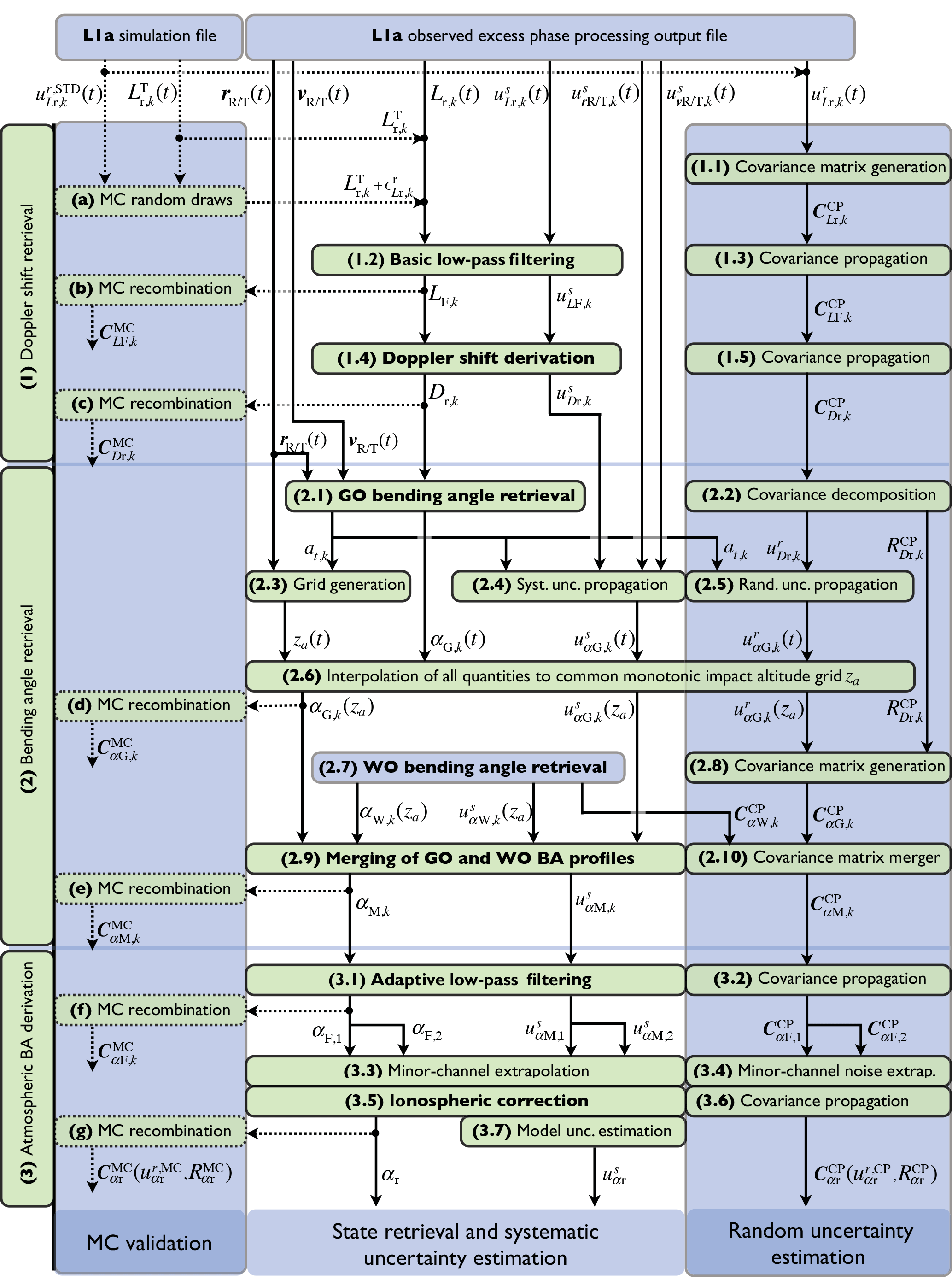
Figure 2Detailed workflow for state retrieval and uncertainty propagation of the main L1b operators from excess phase to atmospheric bending angle profiles (1)–(3) and of the subroutines used in the MC testing framework (a)–(g). The mathematical notation, including all symbols, is introduced in Tables 1 and 2.
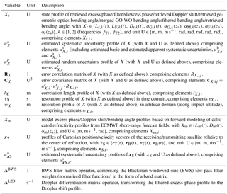
Table 1Principal variables for the rOPS L1b uncertainty propagation.
This study is a direct complement to the work in SKS2017. Using the same propagation and validation methods as applied in SKS2017, it focuses on the uncertainty propagation from excess phase to atmospheric bending angle profiles, i.e., the L1b processing. As in SKS2017, random uncertainties are propagated using covariance propagation (CP) and validated using Monte Carlo (MC) ensemble methods. As in the L2a processor, we also propagate (conservative bound) estimates for systematic uncertainties along the retrieval chain of the L1b processor. Additionally, correlation length profiles and resolution profiles are provided.
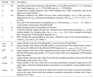
Table 2Vertical grids, coordinate variables, and specific settings for the rOPS L1b processing system.
Uncertainty propagation as covariance propagation from excess phase to bending angle profiles has been outlined and demonstrated in a basic form, by Syndergaard (1999) and Rieder and Kirchengast (2001), but not been implemented yet in processing center retrieval chains or applied to real RO data. As visible in Fig. 1, the L1b processor consists of three major retrieval parts, which are expanded into detailed substructure in Fig. 2. We propagate estimated random uncertainties from excess phase profiles to Doppler shift profiles (Sect. (1) in Fig. 2); further to geometric-optics (GO) bending angle profiles, merged with wave-optics (WO) bending angle profiles (2); and finally to atmospheric bending angle profiles (3), using a full-CP approach. In combination with the definitions of the main operators and variables in Table 1, and of the vertical grid and coordinate variables in Table 2, Fig. 2 provides a concise overview on the detailed workflow of the L1b processor.
Uncertainty propagation for the WO bending angle retrieval has been implemented and demonstrated for simulated events by Gorbunov and Kirchengast (2015); estimation of random and systematic uncertainties for real events including boundary layer bias correction is introduced by Gorbunov and Kirchengast (2018).
Other ongoing rOPS retrieval advancements relevant to this study are the inclusion of the high-altitude initialization algorithm, introduced by Li et al. (2013, 2015), in the L2a processor and the reduction of remaining higher-order ionospheric effects in the retrieved bending angle profiles of the L1b processor (based on work by Syndergaard, 2000; Liu et al., 2015; Healy and Culverwell, 2015; and Danzer et al., 2013, 2015). Furthermore, the precise orbit determination (POD) of the RO receiver satellite and the excess phase processing, also including the associated uncertainty propagation, are part of ongoing work (Innerkofler et al., 2017).
Finally, related work and manuscript preparation on a new moist-air retrieval algorithm (L2b) and corresponding L2b uncertainty propagation are ongoing (Li et al., 2018; Kirchengast et al., 2017a).
The paper is structured as follows. In Sect. 2 we introduce the uncertainty estimation, propagation, and validation methods and the data sources and preparation. In Sect. 3, with the help of an example RO event, the uncertainty propagation sequence is introduced. In Sect. 4 we present the results from the MC validation of the CP uncertainty estimates. In Sect. 5 the performance of the algorithm is then evaluated using test day ensembles with real data from the RO missions CHAllenging Minisatellite Payload (CHAMP) (Wickert et al., 2001); FORMOSAT-3 Constellation Observing System for Meteorology, Ionosphere, and Climate (COSMIC) (Anthes et al., 2008); and Meteorological Operational Satellite A (MetOp) (Luntama et al., 2008); as well as with simulated data approximating characteristics of the Meteorological Operational Satellite A (Luntama et al., 2008; simMetOp data hereafter). We close with conclusions and outlook in Sect. 6. A detailed description of the implemented uncertainty propagation algorithms can be found in Appendix A.
2.1 Methods
We follow the Guide to the Expression of Uncertainty in Measurement (JCGM, 2008a, b, 2011; GUM hereafter) and aim to follow terminology as provided by the International Vocabulary of Metrology (JCGM, 2012), a terminology also adopted by the GUM. SKS2017 provides a more thorough introduction, including the motivation for using the respective uncertainty estimation, propagation, and validation methods; we refer the particularly interested reader to this companion (open-access) work and provide the essential methods needed more in a summarized form below.
We categorize uncertainties into estimated random uncertainties and estimated systematic uncertainties. Effects of unpredictable or stochastic temporal and spatial variations in repeated observations, like effects from fluctuations in the atmosphere or the thermal noise of the receiver system, could in principle be estimated by ensemble statistics from multiple RO events. However, since such effects are essentially stationary in a statistical sense, we can estimate their statistics also from individual RO event data, given their high noise-resolving sampling rate. These effects are included in the estimated random uncertainties.
Systematic effects (biases), which can not be quantified using statistical data analysis based on just one individual RO profile, are estimated and corrected for when known, as recommended by the GUM. The remaining residual biases are assumed to stay within a (conservative) bound estimate, which we refer to as estimated systematic uncertainty and by which we aim to provide at least 90 % likelihood coverage (confidence) that residual biases stay within the plus/minus envelope range of this uncertainty.
Depending on their nature, components of the systematic uncertainty that we need to estimate can be fundamentally systematic across different RO events, a subtype we term estimated basic systematic uncertainties, or appear systematic just for individual RO events, a second subtype that we term estimated apparent systematic uncertainties. It is important to distinguish these two subtypes, since the apparent systematic uncertainties will essentially behave as random uncertainties in ensemble averaging over many RO events, such as when generating climatologies, while the basic systematic ones will not average out and therefore fundamentally limit the (absolute) accuracy of ensemble averages such as climatologies.
Since the noise-type effects giving rise to short-range-correlated random uncertainties can be considered uncorrelated to the bias-type effects inducing long-range-correlated apparent systematic uncertainties, and since both are uncorrelated to basic systematic uncertainties, it is insightful and possible with due care to estimate and propagate each of these uncertainties independently.
As for the L2a processor (SKS2017), the operators of the L1b processor (i.e., the boldfaced items 1.2, 1.4, 2.1, 2.7, 2.9, 3.1, and 3.5 in Fig. 2) qualify as explicit, multivariate, and linear measurement models, as defined in the GUM, with correlated input quantities. They can therefore be formulated as
where the input quantity X and output quantity Y are rank 1 vectors (profiles) of random variables, which we call state profiles. According to the GUM, their random uncertainties can be propagated using
when the uncertainties are normally distributed. This assumption is reasonably justified, since the receiving system noise (i.e., thermal noise and residual clock estimation noise) and the ionospheric noise (from scintillations induced by ionospheric irregularities) are essentially normally distributed overall (Kursinski et al., 1997; Syndergaard, 1999; Gorbunov, 2002b; Sokolovskiy et al., 2009). These noise sources are the main contribution to the random uncertainties in the excess phase profiles feeding into the L1b processor.
CX and CY are the covariance matrices of the input and output variables, respectively, and AXY is the linear (or linearized) operator connecting X and Y. Equation (3) formulates how the covariance matrix CX is calculated from random uncertainty estimates and the correlation matrix RX:
As a key variable characterizing RX, correlation length profiles lX are estimated from the correlation functions assembled in RX. The algorithm used estimates lX by searching for the distances downward and upward of the correlation functions' main peak at which the correlation function has dropped to a value of 1∕e (≈0.378). The adopted correlation length estimate is the arithmetic mean of these two upward and downward estimates (as the peak may be somewhat asymmetric). Additionally the correlation length is constrained by the data domain; i.e., the correlation length can never be larger than the profiles' vertical range.
Since the covariance propagation of random uncertainties requires extensive matrix multiplications for each measurement model along the entire retrieval chain, we also tested simpler variance propagation (VP), for which correlations are ignored; Appendix B summarizes the relevant algorithms. However, as shown in Sect. 4, variance propagation unduly overestimates random uncertainties, so that covariance propagation is required.
When the operator is linear, as is the case for the applicable L1b operators, estimated systematic uncertainties can be propagated by application of the state retrieval operator on the estimated systematic input uncertainty:
where and are the rank 1 systematic uncertainty profiles of the input and output variables.
In addition to random uncertainties, systematic uncertainties, and the correlation length, we also estimate resolution profiles wX as context information along with the provided random uncertainty profiles (necessary, e.g., because smoothing can decrease random uncertainties, while making resolution coarser). This is enabled by careful selection and formulation of low-pass filter operations, in particular explicit filter cutoff frequency specification as the main driver of the resolution remaining after low-pass filtering.
We note that the (half-)Fresnel scale physical resolution often ascribed to RO bending angle profiles retrieved by geometric-optics methods (e.g., Kursinski et al., 1997; Gorbunov et al., 2004) will generally be somewhat coarser than the filter-limited resolution estimated here. This is intentional to maximize available information in the bending angle profiles provided by the L1b processor. In the rOPS, on input to the L2a processor and before high-altitude initialization by statistical optimization, the resolution of all profiles is brought to a common altitude-dependent resolution, which reflects the half-Fresnel scale (SKS2017).
2.2 Data sources and preparation
The input variables needed for the L1b uncertainty propagation, visible in Fig. 2 and defined in Table 1, are the retrieved excess phase profiles Lr,k(t) and the associated systematic uncertainty profiles , random uncertainty profiles , and correlation matrices , as well as the orbit positions and velocities of receiver and transmitter satellite – rR(t), vR(t), rT(t), and vT(t) – and their (systematic) uncertainties, , , , and . For due limitation of depth of workflow detail in Fig. 2 we do not separately show the propagation of the basic and apparent systematic uncertainties as they are both identically propagated through the operator chain shown for . All variables are provided on the time grid t with elements ti, at fs=50 Hz sampling rate, and for the two GPS carrier frequencies: fTk, with , fT1=1.57542 GHz, and fT2=1.22760 GHz.
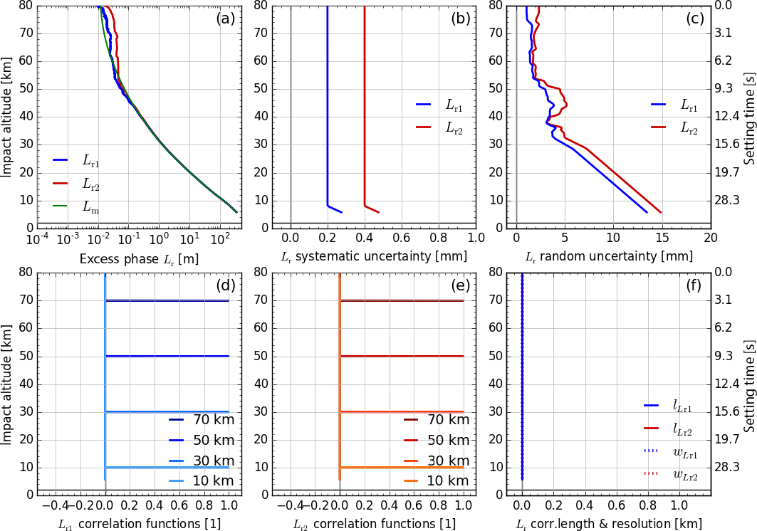
Figure 3Input profiles of retrieved excess phase Lr (with model profile Lm for comparison) in panel (a), estimated systematic uncertainty profiles in panel (b), estimated random uncertainty profiles in panel (c), representative correlation functions RLr,i (at 10, 30, 50, and 70 km) in panels (d) and (e), and correlation length lLr (solid) and resolution profiles wLr (dotted) in panel (f), which are set zero for these initial essentially uncorrelated input data. All profiles are shown for both GPS carrier frequencies: fT1 (blue) and fT2 (red).
We used excess phase state profiles Lr,k(t) and the orbit state profiles rR(t), vR(t), rT(t), and vT(t) from 15 July 2008 as a test day ensemble. For CHAMP, COSMIC, and MetOp, orbit state and excess phase profiles were provided by the COSMIC Data Analysis and Archiving Center (CDAAC) of the University Corporation for Atmospheric Research (UCAR), Boulder, Colorado. The End-to-End GNSS Occultation Performance Simulation and Processing System (EGOPS) (Fritzer et al., 2009) was used for generating the simulated MetOp orbit state and excess phase profiles with realistic receiver noise (simMetOp). Figure 3 shows Lr,k(t) in panel (a), in panel (b), in panel (c), and in terms of representative correlation functions in panels (d) and (e), for a typical COSMIC RO event of the test day ensemble from 15 July 2008 (example case).
Exploiting the linearity of the (linearized) retrieval operators, the so-called baseband approach (Kirchengast et al., 2016a) is applied throughout the rOPS. Hereby a zero-order model profile is subtracted from the input state profile, and only the remaining delta profile is processed through the operator. After application of the operator, the zero-order model profile of the output state profile is added back to the resulting delta profile. This approach effectively avoids biases from numerical operations on (near-)exponentially varying RO profiles, since the model profiles that we derive from short-range (24 h) forecasts of the European Centre for Medium-Range Weather Forecasts (ECMWF) skillfully subtract the (near-)exponential variation. The remaining increment profiles that we need to treat numerically then appear to be very linear and with low dynamical range, which leads to very low residual numerical errors of operators such as filters and derivatives.
The model profiles used as zero-order states in the retrieval – i.e., Lm, Dm, and αm (cf. Table 1) – were created from ECMWF short-range (24 h) forecast refractivity fields, accurately forward-modeled to bending angle (αm), Doppler shift (Dm), and excess phase (Lm) profiles, collocated to the latitude, longitude, and time of the respective RO event processed in the rOPS. The ECMWF fields used have a horizontal resolution of about 300 km (triangular truncation T42) – which corresponds to the approximate horizontal resolution of RO profiles (e.g., Kursinski et al., 1997) – and are available at 91 vertical levels (L91).
ECMWF fields were chosen for their proven leading quality (Untch et al., 2006; Bauer et al., 2015) and thus high suitability for serving as zero-order state profiles; any other reasonable model profiles could be used as well since the retrieval results negligibly depend on the exactly chosen zero-order model profiles. For comparison we plotted Lm(t) for the COSMIC example case into Fig. 3a, which demonstrates that the ECMWF short-range forecast lies very close to Lr1(t) and Lr2(t) and thus is well suited as the model profile.
While in the future the excess phase random and systematic uncertainty profiles will be more rigorously estimated by the rOPS L1a processor (Innerkofler et al., 2017) and provided as input to the L1b processor, they had to be estimated for this study from existing excess phase profiles with realistic noise and simplified modeling. To this end, each estimated random uncertainty profile was estimated based on the noise of the respective retrieved excess phase profile Lr,k(t). The noise was determined following the estimation scheme for bending angle observation errors described by Li et al. (2015, Sect. 2.2 therein), so we just briefly summarize how we used it here.
First, for both, the retrieved profile Lr,k and for the model profile Lm, the mean over all grid points between 60 and 70 km was determined. Then Lm was offset-corrected towards Lr,k by subtracting the difference of these two means from Lm, giving the offset-corrected model profile . Next, the delta profile was calculated. After smoothing with a 10 km moving-average boxcar (BC) filter, the smoothed profile was subtracted from again, to get , the random noise profile component of Lr,k isolated in this way. Finally, the estimated random uncertainty was determined as
where M is the number of grid points equivalent to a window width of 10 km. To avoid boundary effects of the filter, was only determined up to zaTop−5 km and down to zaGradr at 30 km. It was constantly extended at the upper end and extended by a linear gradient below zaGradr, using (in units [m])
for all elements of below zaGradr, roughly following estimates of ESA/EUMETSAT (1998) and the overall behavior of estimates from real excess phase profiles (the latter became too vulnerable to biases and fluctuations to continue using them below 30 km).
Since the noise components responsible for the random uncertainty at excess phase level are essentially uncorrelated at a sampling rate of 50 Hz (Syndergaard, 1999; Hajj et al., 2002), the correlation matrix RLr is set to unity in the diagonal and to zero outside (i.e., a Kronecker-δ assignment) for both channels (Fig. 3d–f). In case the future excess phase data from the rOPS L1a processor exhibit non-negligible correlations for some data from some of the RO missions, we will account for these correlations in RLr, since our L1b algorithm (Sect. 3) is prepared for full covariance propagation. The elements of the covariance matrix CLr are hence (item 1.1 in Fig. 2)
For the MC validation of the CP, error profile realizations were superimposed onto simulated “true” excess phase profiles . As a source for , we used an EGOPS-simulated “error-free” CHAMP event from 8 August 2008 (i.e., no receiver system errors superimposed). Using an “error-free” profile as the basis, with the particular simulated profile just serving as a representative RO profile to illustrate the MC validation, allows us to strictly ensure the consistency of the random uncertainty of the input profile with the ensemble of superimposed error profile realizations.
To create the error profiles, a representative uncertainty profile was selected from a COSMIC ensemble of uncertainty profiles, created according to Eqs. (5) and (6). The error profile realizations are random draws from a distribution characterized by these uncertainties, again assuming that , i.e., that there are no correlations between the individual grid levels (item (a) in Fig. 2; Fig. 3f). The same standard profile was used as input for the CP to which the MC results are then compared. This MC validation method applied to test the rOPS L1b uncertainty propagation steps is essentially the same as in SKS2017, and it is described therein in more detail.
The estimated systematic uncertainty was determined based on a simple model roughly following error estimates from ESA/EUMETSAT (1998), with constant uncertainty from 80 km down to zaGrads at 8 km and a linear uncertainty gradient in the troposphere; as noted above, this simplified modeling will be replaced in the future by realistic uncertainty estimates received as L1b retrieval input from the L1a processor (Innerkofler et al., 2017).
The constant above zaGrads is 0.1 mm for k=1 and 0.2 mm for k=2 for MetOp and simMetOp. This uncertainty is interpreted as an estimated basic systematic uncertainty, i.e., as a lower-bound estimate of available accuracy.
For CHAMP and COSMIC we set mm and mm, to roughly reflect the fact that these RO receivers are lower-cost instruments with lower gain, and thus somewhat lower tracking performance, than the RO receiver on MetOp (e.g., Luntama et al., 2008; Angerer et al., 2017). From zaGrads downwards, (in units [m]) increases by
In order to avoid a sharp kink in the profiles at zaGradr, and in the profiles at zaGrads, a 2 km width moving-average boxcar filter was applied to smooth these simple uncertainty models around these transition altitudes (for the example profile is visible in Fig. 3b).
The orbit position and velocity uncertainties of the transmitter and the receiver satellites show little variation within the short duration of an individual RO event of about 45 s to 2 min (Innerkofler et al., 2017) and can be assumed to be constant biases. They are thus counted to the systematic uncertainties, more precisely the apparent systematic uncertainties, since the actual values of the orbit-borne biases will generally change in a pseudo-random manner from event to event.
We set the transmitter position and velocity uncertainties to cm and mm s−1, consistent with accuracies for GPS orbits available from GNSS orbit providers like the International GNSS Service (IGS). The receiver position and velocity uncertainties, cm and mm s−1 for CHAMP and MetOp, are adopted 4 times smaller than those for COSMIC with cm and mm s−1, as found by ongoing rOPS-related POD studies (Innerkofler et al., 2017), consistent with previous literature (e.g., Montenbruck et al., 2009; Schreiner et al., 2010).
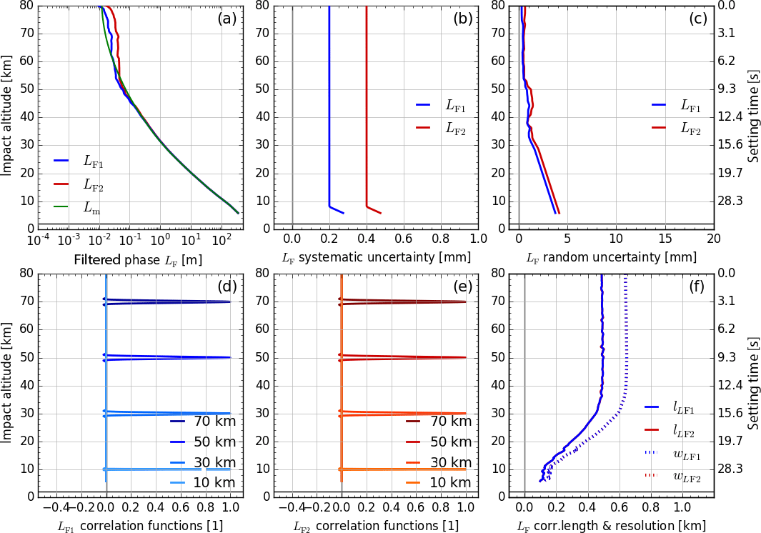
Figure 4Results for filtered excess phase profiles LF (with model profile Lm for comparison) in panel (a), estimated systematic uncertainty profiles in panel (b), estimated random uncertainty profiles in panel (c), representative correlation functions RLF,i (at 10, 30, 50, and 70 km) in panels (d) and (e), and correlation length lLF (solid) and resolution profiles wLF (dotted) in panel (f). All profiles are shown for both GPS carrier frequencies: fT1 (blue) and fT2 (red).
In this section the L1b uncertainty propagation algorithm sequence is introduced. We illustrate the effects of the algorithm on the main uncertainty variables by way of the COSMIC example case already used for Fig. 3.
For each L1b retrieval step – i.e., segments (1), (2), and (3) in Fig. 2 – the results for the principal variables are shown in Figs. 4 to 8. These variables are the state profiles Xr (with , Dr,k(t), αG,k(t), αG,k(za), αM,k(za), αF,k(za), and αr(za)}), the estimated systematic uncertainty profiles , the estimated random uncertainty profiles , representative correlation functions RXr,i (with i such that ), and the correlation length profiles lXr and resolution profiles wXr. Along with the dual-frequency state profiles, we also show the collocated forward-modeled short-range forecast profiles, i.e., model profiles Xm with for comparison.
A concise definition of the variables involved is provided in Table 1, as introduced above. The summary description in this section is complemented by a complete step-by-step description of the algorithm along the entire L1b retrieval chain in Appendix A, which is organized for convenience into the same sequence of subsections.
To simplify the notation in the description, we suppress index k whenever steps are applied in an identical way to the data of both GNSS L-band channels with frequencies fT1 and fT2. Only if the two channels are treated differently, such as in Sect. 3.3, is the index considered again. For conciseness we also do not illustrate both the estimated basic and estimated apparent systematic uncertainty but rather the total estimated systematic uncertainty as the overall result.
3.1 Doppler shift retrieval
3.1.1 Basic low-pass filtering
A Blackman windowed sinc (BWS) low-pass filter with a filter cutoff frequency fc=2.5 Hz (boxcar-equivalent filter width of 0.2 s) (item 1.2 in Fig. 2) is applied onto the excess phase profile Lr(t), before the Doppler differentiation (item 1.4 in Fig. 2), to avoid an amplification of high-frequency noise in the phase profile by the derivative operation. This filter suppresses the noise; consequentially the filtered excess phase profile LF(t), shown in Fig. 4a, is expected to have random uncertainties of smaller magnitude, but correlated over the length of the filter window. The uncertainties obtained through the implemented algorithm confirm these expectations, i.e., random uncertainty profiles in Fig. 4c are less than a third in magnitude of those in Fig. 3c, and Fig. 4d–e show how the correlation functions widened and the correlation length and vertical resolution reached ∼0.5 and ∼0.6 km, respectively, above about 30 km impact altitude (Fig. 4f).
The random uncertainty propagation algorithm, i.e., the covariance propagation from CLr to CLF, is described by Eq. (A6) and item 1.3 in Fig. 2 and is justified by Eq. (2). To obtain and RLF, we use Eqs. (A7) and (A8).
To propagate the estimated systematic uncertainty , which characterizes long-range-correlated offsets or biases, we use the same BWS filter as for the state profile, i.e., making use of Eq. (4). Because the input uncertainty profile is chosen to be constant down to zaGrads, the filter has little effect, and , shown in Fig. 4b, is essentially equal to , shown in Fig. 3b.

Figure 5Results for retrieved Doppler shift profiles Dr (with model profile Dm for comparison) in panel (a), estimated systematic uncertainty profiles in panel (b), estimated random uncertainty profiles in panel (c), representative correlation functions RDr,i (at 10, 30, 50, and 70 km) in panels (d) and (e), and correlation length lDr (solid) and resolution profiles wDr (dotted, estimated for main peak) in panel (f). All profiles are shown for both GPS carrier frequencies: fT1 (blue) and fT2 (red).
The resolution profile wLr is determined by the filter width according to Eqs. (A11) and (A13). After the BWS filtering, the resolution is roughly equal to the correlation length lLF, amounting to ∼0.6 km above about 30 km impact altitude and becoming finer downwards due to the increasing refraction (Fig. 4f).
3.1.2 Doppler shift derivation
The next step is a five-point differentiation operation (item 1.4 in Fig. 2) used to calculate the Doppler shift profile Dr(t) from the filtered excess phase profile LF(t). The resulting dual-frequency Doppler shift profiles are plotted along with the model profile Dm(t) in Fig. 5a for the example case.
As for the filtered excess phase, we apply CP (Eq. A18, item 1.5 in Fig. 2) to first calculate the covariance matrix CDr and then extract (shown in Fig. 5c) and RDr (Fig. 5d and 5e) from it. The choice of the x-axis range shows the random uncertainties increased, but the differentiation actually does increase relative random uncertainties (relative to the state profile). It also causes anti-correlation with neighboring elements, as visualized by the negative side peaks of the correlation functions in Fig. 5d and 5e. The correlation length lDr (of the main correlation function peak) decreases accordingly (now smaller than 0.3 km throughout), because the correlation functions fall off more steeply on both sides of the main peak (Fig. 5f).
For calculating the estimated systematic uncertainty, we use the state operator; i.e., we just differentiate and get (shown in Fig. 5b). With the current illustrative choice of input uncertainties the systematic uncertainty of the Doppler shift profile is zero above the transition to the troposphere, where the estimated systematic uncertainty of the excess phase is assumed constant; in the troposphere a Doppler shift offset of ∼ 0.02 mm s−1 occurs.
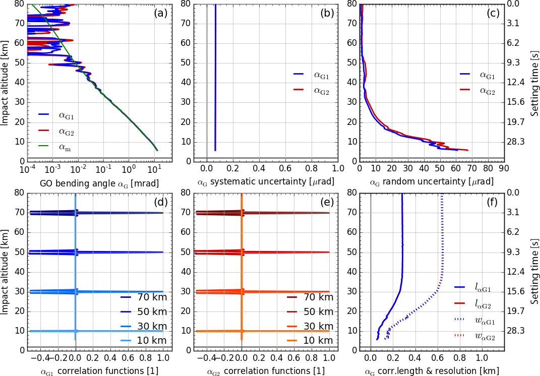
Figure 6Results for geometric optics bending angle profiles αG (with model profile αm for comparison) in panel (a), estimated systematic uncertainty profiles in panel (b), estimated random uncertainty profiles in panel (c), representative correlation functions RαG,i (at 10, 30, 50, and 70 km) in panels (d) and (e), and correlation length lαG (solid) and resolution profile wαG (dotted, estimated for main peak) in panel (f). All profiles are shown for both GPS carrier frequencies: fT1 (blue) and fT2 (red); in panels (b) and (f) both profiles are essentially identical (so that blue shadows the red color).
The resolution profile wDr shows that the vertical resolution stays unaffected by this operator (cf. Figs. 5f and 4f), because the BWS filter width of the preceding low-pass filtering (intentionally) stretched beyond the five neighboring points involved in the differentiation.
3.2 Bending angle retrieval
3.2.1 GO bending angle retrieval
The next operator is the GO bending angle retrieval in which retrieved GO bending angle profiles αG(t) are calculated from Doppler shift profiles Dr(t) and the orbit position and velocity vectors rT(t), rR(t), vT(t), and vR(t) (item 2.1 in Fig. 2) and then interpolated to the (common monotonic) impact altitude grid za (item 2.6 in Fig. 2).
Figure 6a shows retrieved αG profiles together with the model profile αm. The mildly nonlinear implicit-type bending angle retrieval operator needs to be solved iteratively, and it requires linearization for both random and systematic uncertainty propagation, as described in detail in Appendix A (Sect. A2). Because this retrieval step is performed level by level, keeping levels independent, the GO bending angle retrieval leaves correlation functions and resolution unchanged (cf. Figs. 6d–f and 5d–f).
The estimated random uncertainties , as shown in Fig. 6c, now increase more strongly in the lower stratosphere and troposphere (to about 40 to 50 µrad near 10 km), because they are dependent on the vertical gradient of the impact parameter at, which is increasingly larger towards lower altitudes from the increasing refraction.
The main contributions to the estimated systematic uncertainty are induced by systematic uncertainties in orbit velocity and position of the transmitter and the receiver satellite (details in Sect. A2), which in total amount to about 0.05 µrad (Fig. 6b). Compared to this magnitude, the systematic uncertainty contributed by the Doppler shift uncertainty is very small.
3.2.2 WO bending angle retrieval
Due to strong refractivity gradients and multipath effects, the GO bending angle retrieval can be inadequate in the troposphere, and therefore WO algorithms are applied to reconstruct the geometric optical ray structure of the wave field (e.g., Gorbunov, 2002a; Gorbunov and Lauritsen, 2004).
In the rOPS, along with the WO bending angle profile αW(za), the systematic uncertainty profile , the random uncertainty profile , the correlation matrix RαW, and the resolution profile wαW are retrieved (item 2.7 in Fig. 2).
The WO bending angle retrieval algorithm used is a canonical transform (CT2) algorithm (Gorbunov et al., 2004), and the associated uncertainty propagation algorithm is not described here, but separately by Gorbunov and Kirchengast (2015, 2018). The WO retrieval and uncertainty propagation results are supplied up to 20 km impact altitude by the WO algorithms.
3.2.3 Merging of GO and WO bending angle profiles
In the rOPS bending angle retrieval the results from the WO retrieval, αW, are merged with GO retrieval results, αG, at around a transition altitude in a transition range , to get merged profiles αM (item 2.9 in Fig. 2). The determination of the transition altitude and the merging algorithm are described in Appendix A2.3. We use a specialized covariance propagation to propagate the GO and WO uncertainties, expressed by the covariance matrices CαG and CαW, to properly obtain the covariance matrix of the merged bending angle CαM (Eqs. A37 and A38, item 2.10 in Fig. 2).
Because the rOPS implementation of the WO uncertainty propagation (Gorbunov and Kirchengast, 2018) was still in test phase and not yet available for integration into the simulations here, all examples in this study are GO-only; i.e., only the GO retrieval is performed. Results for αM are thus unchanged from those shown in Fig. 6 and not separately illustrated.
In order to nevertheless test and validate the uncertainty propagation of the merging algorithm, WO retrieval results were artificially substituted by the GO results for the MC validation (Sect. 4); i.e., GO was used as a proxy for WO since reasonably capturing expected WO variability as indicated by tests of Gorbunov and Kirchengast (2018).
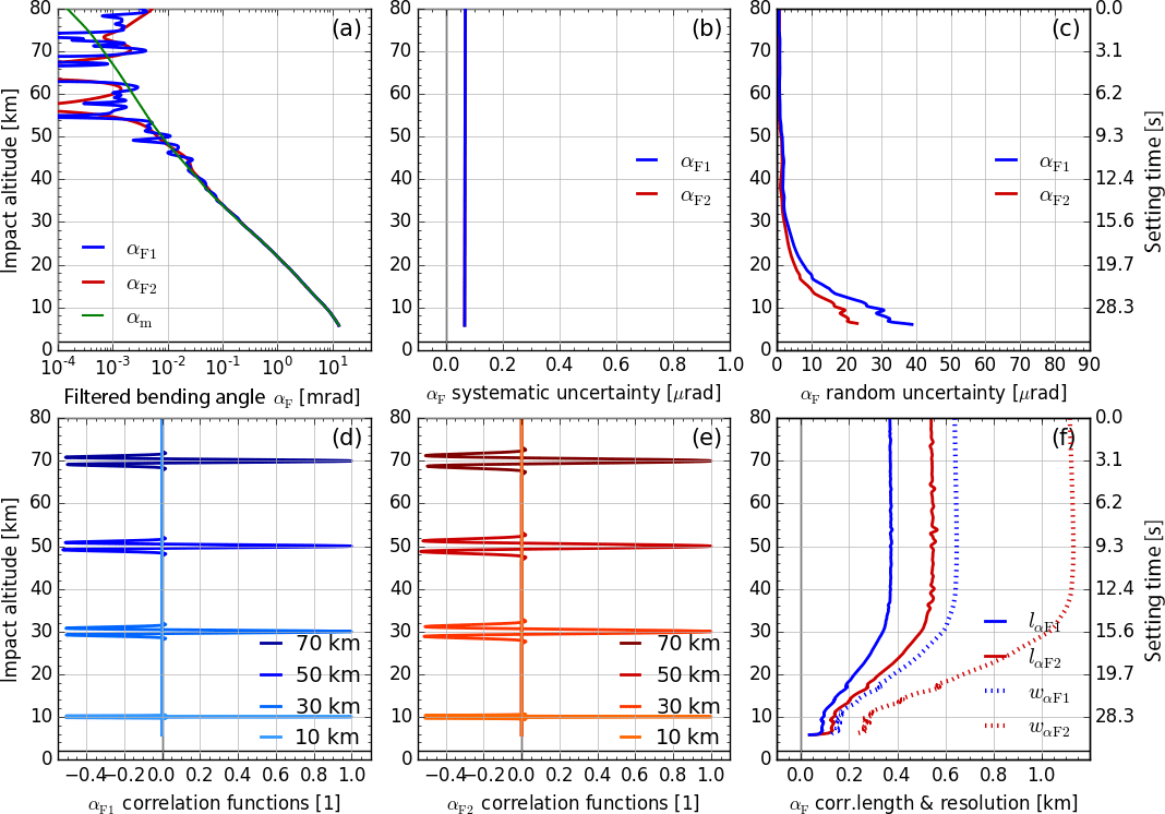
Figure 7Results for filtered bending angle profiles αF (with model profile αm for comparison) in panel (a), systematic uncertainty profiles in panel (b), random uncertainty profiles in panel (c), representative correlation functions RαF,i (at 10, 30, 50, and 70 km) in panels (d) and (e), and correlation length lαF (solid) and resolution profiles wαF (dotted, estimated for main peak) in panel (f). All profiles are shown for both GPS carrier frequencies: fT1 (blue) and fT2 (red).
3.3 Atmospheric bending angle derivation
3.3.1 Adaptive low-pass filtering and minor-channel extrapolation
To prepare the merged bending angle profiles αM,k for the ionospheric correction, they are first filtered by another BWS filter operation (item 3.1 in Fig. 2) in order to ensure adequately smoothed bending angle profiles αF,k, with .
The chosen filter cutoff frequency for k=1 is fc1=2.5 Hz, same as the basic filtering (Sect. 3.1.1), just to ensure clearness of any higher-frequency effects from operators after the initial excess phase filtering (e.g., from Doppler shift derivation that induces short-range anti-correlation effects). For k=2, the cutoff frequency fc2 is set noise-dependent, between 2.5 and 0.5 Hz (boxcar-equivalent width of 0.2 to 1.0 s). In events in which the αF2 profile does not reach down as far as αF1, it is extrapolated down to the bottom of αF1, zaBot. The results for the filtered bending angle state profiles αF,k are displayed in Fig. 7a, together with the associated model bending angle profile αm. The filter has considerably reduced the noise of the profile, particularly for αF2, where the algorithm selected a cutoff frequency Hz in this example case.
The relevant covariance-propagated random uncertainties are shown in Fig. 7c (blue and red), illustrating the reduced noise, especially for αF2. In return, the peaks of the correlation functions broaden (cf. Figs. 7d–e and 6d–e), with correlation lengths lαF,k at near 0.4 km for αF1 and above 0.5 km for αF2 (Fig. 7f).
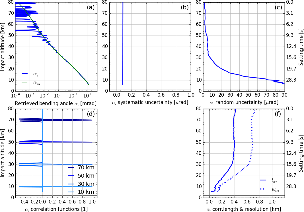
Figure 8Results for atmospheric bending angle profile αr (with model profile αm for comparison) in panel (a), systematic uncertainty profile in panel (b), random uncertainty profile in panel (c), representative correlation functions Rαr,i (at 10, 30, 50, and 70 km) in panel (d), and correlation length lαr (solid) and resolution profile wαr (dotted, estimated for main peak) in panel (f).
The estimated systematic uncertainty remains largely unchanged (Fig. 7b) due to its smooth character.
The resolution of the filtered bending angle profiles (according to Eqs. A11 and A13) is determined by the cutoff frequencies fc,k of the BWS filters. In the example case it is therefore essentially unchanged for αF1, while it is significantly decreased for αF2 (cf. Figs. 7f and 6f) since Hz. That is, the resolution wαF2 in the upper stratosphere for example, where the vertical scanning velocity of this RO event is about 3.2 km s−1, is near 1.1 km (Fig. 7f).
3.3.2 Ionospheric correction
The final step of the L1b processor is the ionospheric correction (item 3.5 in Fig. 2). The atmospheric bending angle αr is obtained by applying a linear dual-frequency combination of αF1 and αF2, such that ionospheric effects are largely removed (details are described in Sect. A3). The final retrieved atmospheric bending angle αr of the example case is shown in Fig. 8a. The propagation results for the estimated random uncertainty are shown in Fig. 8c. The linear combination of the ionospheric correction amplifies noise and is therefore considerably larger than , and (cf. Figs. 8c and 7c).
Figure 8d shows how the correlation functions – as obtained through covariance propagation – combine the characteristics of the correlation functions from the two matrices RαF1 and RαF2, while essentially inheriting the αF1 behavior, since the αF2 influence on the ionospheric correction is comparatively minor (see Sect. A3).
The residual higher-order ionospheric effects are accounted for by a “conservative best-guess” value (0.05 µrad, reflecting results of Liu et al., 2015, and Danzer et al., 2013, 2015) and added (in root-mean-square form) to the systematic uncertainty profile , leading to a total estimated systematic uncertainty in this example case of ∼ 0.07 µrad (Fig. 8b). Within this uncertainty, the one dominating component from orbit uncertainties (∼ 0.05 µrad; cf. Fig. 6b) can be considered an apparent systematic uncertainty that will essentially average out in ensemble averaging (e.g., climatologies), while the other dominating component from residual higher-order ionospheric biases (also estimated ∼ 0.05 µrad as noted above) can be considered a basic systematic uncertainty. For the latter it is therefore useful and prepared for in the rOPS – in line with GUM recommendations and as discussed in the introductory Sect. 1 – to correct for the quantifiable part of it in the future so that the total basic systematic uncertainty may be mitigated down to the ∼ 0.01 µrad level.
The resolution profile wαr of the retrieved bending angle (Fig. 8f) is dominated by the contribution of αF1 that strongly dominates (intentionally by construction) the ionospheric correction results in terms of the small-scale bending angle variability. Similar to the correlation length profile lαr, it is therefore very close to wαF1 and only slightly larger.
The GUM advises to use a MC method for uncertainty propagation if the retrieval operators do not fulfill the criteria for a GUM-type CP. In our case the MC method is put to another beneficial use, to validate the results of the CP, as recommended by JCGM (2011).
For the validation of the covariance propagation by the MC method, we sampled the input excess phase profile random error distribution, statistically described by
by a large number M of draws (with and M=1000). For each of these M profile realizations, the state retrieval is run through the L1b retrieval chain, to give M realizations of the output variable Xj (with and ). From these individual realizations the mean profiles XMC and the covariance matrices ,
are calculated (items b–g in Fig. 2). Using the same input profile and uncertainty information as used to specify the MC runs (described in Sect. 2.2), the retrieval is then also run with covariance-based uncertainty propagation, and the resulting CP-propagated covariance matrices are compared to the MC-derived matrices . In order to be able to attribute potential changes between CP and MC covariance matrices better, we decompose CX into and RX (Eqs. A7 and A8), and compare them separately.

Figure 9Results from the validation of CP covariance matrices (“CP”) by MC covariance matrices (“MC”) (first four rows): the consecutive retrieval steps are shown for LF (a–c; in panels a–b also for Lr) and Dr (d–f) relative to setting time t, and for αG (g–i) and αF (j–l) relative to impact altitude za. The left column shows estimated random uncertainties for fT1 (CP in blue, MC in black, in panel a in light blue); the middle column for fT2 (CP in red, MC in black, in panel b in orange); the right column representative correlation functions at 60, 36, and 12 km for fT1 (CP in blue, MC in black) and 72, 48, and 24 km for fT2 (CP in red, MC in black). The last row (m–o) shows CP (blue) and MC (black) results for estimated αr random uncertainties (m) and representative correlation functions at 72, 60, 48, 36, 24, and 13 km (o), as well as variance propagation (“VP”) results (light blue) for αr in panel (n).
Figure 9 shows the different steps along the retrieval chain from LF,k(t) to Dr,k(t), αG,k(za), αF,k(za), and αr(za) in the rows, for k=1 (GPS fT1 frequency) in the left column and for k=2 (GPS fT2 frequency) in the middle column. The right column shows multiple representative correlation functions, from near 10 to near 70 km. Due to the limited number of MC draws, the MC results (black lines) show some jitter both in the estimated random uncertainty and in the correlation functions. Since the purpose of the MC results is only to demonstrate the correctness of the CP result, we can disregard this behavior.
Figure 9a (light blue) and b (orange) show the random uncertainties and , respectively, which characterize the input distribution and from which the random error profiles are drawn. They also show the CP results for the random uncertainty (dark blue in Fig. 9a) and (red in Fig. 9b), compared to the MC propagated random uncertainties (black).
The CP and MC lines match very well and show that the implemented CP algorithm delivers correct results for the basic filtering step. For fT2, the MC uncertainties do not reach down as far as the CP uncertainties, because the shortest of all draws of the large ensemble of size M determines how far down the recombined MC covariance matrix (Eq. 10) reaches. Figure 9c compares CP correlation functions RLF,i1 (blue) and RLF,i2 (red) to the corresponding MC correlation functions (black dashed).
The CP and MC correlation functions also agree well. Both capture the narrow peak, broadened by the BWS filter. Again the MC correlation functions fluctuate around zero left and right of the peak, from the finite ensemble size, but it is obvious that the CP delivers the correct off-peak results (i.e., zero; the off-peak elements outside the BWS filter window must nominally be zero). The MC validation (black) of (Fig. 9d), (Fig. 9e), and RDr,i (Fig. 9f, blue and red) demonstrates that the CP through the Doppler shift derivation performs correctly as well.
The next row, Fig. 9g to i, shows the results for the GO bending angle αG(za), i.e., after the interpolation of all quantities to the (common monotonic) impact altitude grid za. For comparison, in Fig. 9a to f, all quantities have been computed on the common time grid (“setting time” relative to time zero at 80 km altitude) with 50 Hz sampling rate; the corresponding impact altitude of the “true” profile is shown for additional convenience on the right-hand-side (RHS) axis. In Fig. 9g to o, these bending angle quantities have been computed on the impact altitude grid; in these cases therefore the corresponding setting time of the “true” profile is shown for additional convenience on the RHS axis.
The results for the filtered bending angle αF follow in Fig. 9j to l. Also here the MC results match the CP result well. Due to the lower BWS cutoff frequency for αF2, now is smaller than , even though was larger than . Correspondingly the peak of the correlation functions RαF,i2 widened more than those of RαF,i1 (cf. Fig. 9l and i).
Finally, Fig. 9m to o show the CP results for retrieved atmospheric bending angle αr, where Fig. 9n is included as a special cross-comparison in the case of only variance propagation being used instead of CP. Figure 9m and o confirm that CP results are also correct for this final L1b variable, in terms both of random uncertainty and correlation functions.
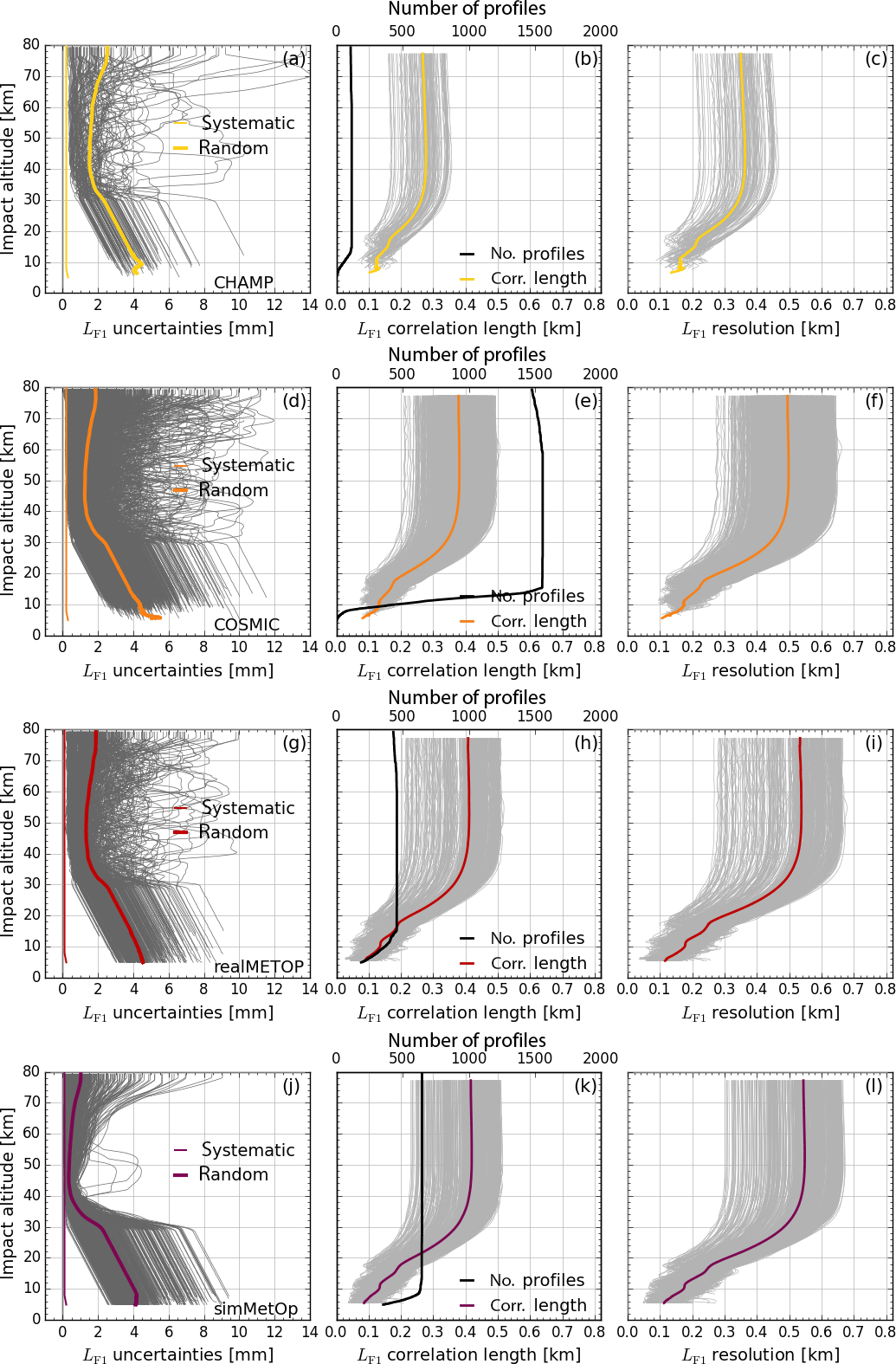
Figure 10Uncertainty propagation results for real-data ensembles from 15 July 2008, for the filtered excess phase profile LF1 of the leading channel (fT1, GPS L1 frequency). Left column: estimated random (heavy) and systematic (light) uncertainty profiles of each ensemble member (gray), and the ensemble mean (color) for CHAMP (a), COSMIC (d), MetOp (g), and simMetOp (j). Middle column: correlation length profiles lLF1 of each ensemble member (gray), the ensemble mean (color), and the ensemble size profile (black, scale at upper axis) for CHAMP (b), COSMIC (e), MetOp (h), and simMetOp (k). Right column: estimated resolution profile wLF1 of each ensemble member (gray) and the ensemble mean (color) for CHAMP (c), COSMIC (f), MetOp (i), and simMetOp (l).
In order to demonstrate that a full CP is necessary to propagate random uncertainties correctly, we also calculated random uncertainties based on mere VP from αG to αr for comparison. A description of this VP algorithm (i.e., only diagonal elements of the covariance matrices are considered) is provided in Appendix B. Figure 9n clearly shows that VP would overestimate random uncertainties in αr considerably, pointing to the importance of the complete CP implementation in the L1b retrieval chain, even though the correlation lengths involved in the processing steps are rather small.
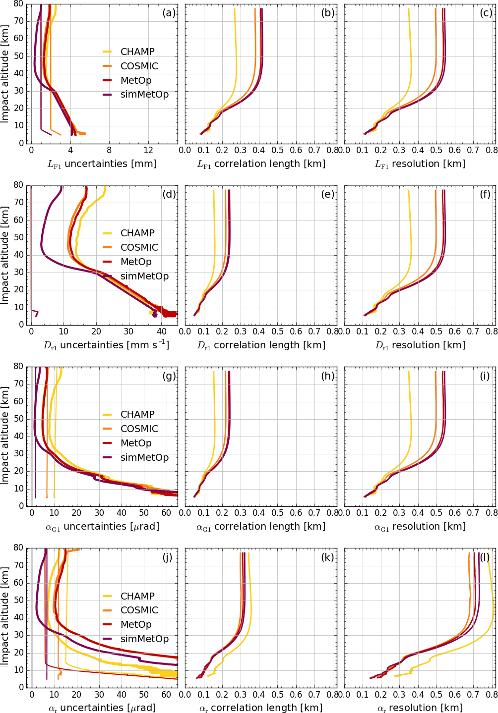
Figure 11Uncertainty propagation results for real-data ensembles from 15 July 2008 for output profiles of the leading channel (fT1, GPS L1 frequency). The first row shows results for LF1 (a–c), the second for Dr1 (d–f), the third for αG1 (g–i), and the fourth for αr (j–l). The different ensemble mean profiles are shown in colors (CHAMP, yellow; COSMIC, orange; MetOp, red; and simMetOp, violet). Left column: mean random uncertainty (heavy) and mean systematic uncertainty (light) profiles (a, d, g, j); the latter is shown as (in a) and (d, g, j) for enabling visibility of these small quantities. Middle column: correlation length profiles lXr (b, e, h, k). Right column: vertical resolution profiles wXr (c, f, i, l).
To statistically evaluate the performance of the new L1b uncertainty propagation algorithm, we also processed a complete test day of real (CHAMP, COSMIC, MetOp) and simulated (simMetOp) data from GNSS RO satellite missions. Figure 10 shows the results for estimated systematic and random uncertainty profiles, as well as correlation length and resolution profiles for filtered excess phase profiles LF,1. Figure 11 subsequently illustrates the ensemble mean of the same variables for LF1, Dr1, αG1, and αr for the test day ensemble. In Fig. 10 we also co-illustrate the number of events processed for each of the RO missions (middle column).
About 5 % of the total number of processed profiles for each mission have been discarded, because they were detected as outliers based on the magnitude of their random uncertainty profiles (these outliers are not included in the number of profiles shown). All profiles are shown as function of impact altitude, because each of the profiles in the ensembles needed to be interpolated to the same (standard) impact altitude grid, to orderly calculate their mean profiles.
Figure 10a shows and for all ∼100 CHAMP events. It is visible (also in Fig. 10d and g) that the random uncertainty is estimated based on excess phase noise between 30 and 75 km and synthetically extended above and below, as described in Sect. 2.2. For the large majority of events, lies between about 0.5 and 3 mm in the range between 30 and 75 km. Note that these results show the random uncertainties after the application of the basic BWS filter (Sect. 3.1.1), but the input uncertainties are of similar shape (though larger in magnitude).
Figure 10b shows that the correlation length profiles of the CHAMP ensemble (gray) and its ensemble mean (yellow) are of relatively constant magnitude from 35 to 80 km but then get smaller downward, because the RO event's scan velocity decreases (see Eq. A13). Since the BWS filter determines the vertical resolution and the correlation length at the same time, the resolution profiles wLF1 (Fig. 10c) are quite similar to the correlation length profiles lLF1 (Fig. 10b).
The number-of-events profile shows that most CHAMP events end between 5 and 12 km (Fig. 10b, black). This is because the GO profiles illustrated here are cut off right at the lower end of the GO–WO transition range at (cf. Table 2).
Compared to CHAMP, the mean random uncertainty (Fig. 10d) for the ∼1500 events of the COSMIC ensemble is smaller, particularly above 30 km, indicating the improved data quality of this later mission. The mean of the correlation length profiles lLF1 (Fig. 10e) is higher than for CHAMP (Fig. 10b), and correspondingly the resolution of the COSMIC profiles is also somewhat coarser (Fig. 10f and c). The cutoff frequency and sampling rate – and thus the resolution in time – are set to be the same in the rOPS, irrespective of the missions; these differences hence are due to the different vertical scan velocities of the missions induced by the differences in orbit altitudes (CHAMP ∼400 km, COSMIC ∼700 km).
For the real MetOp data (available here as a data set from UCAR/CDAAC, as for CHAMP and COSMIC), appears similar to COSMIC (cf. Fig. 10d, g), while for simMetOp (with best possible simulated MetOp-type receiver noise) it is clearly smaller than for COSMIC. From 35 to 80 km the mean random uncertainty profile for simMetOp stays below 1 mm (Fig. 10j). Three individual profiles exhibit comparatively high uncertainties of larger than 2 mm within about 40 to 55 km, however, reflecting that the simMetOp error simulations are capable of partly generating higher-noise profiles of the type more frequently seen in the real MetOp data (Fig. 10g).
On the other hand, the average correlation length/resolution profile of the ∼500 real MetOp and ∼700 simMetOp ensemble members is very similar, driven by the orbit being essentially the same for the real data and the simulations (Fig. 10h, i, k, l). Compared to COSMIC (Fig. 10e, f), the correlation length and resolution are again somewhat larger/coarser, due to an even somewhat higher scan velocity of the MetOp satellite (∼820 km orbit altitude). The systematic uncertainty – just co-illustrated for completeness in Fig. 10a, d, g, and j – is almost left unchanged by the BWS filter and is essentially equal to the preset input uncertainty for all three missions (Sect. 2.2).
Figure 11 shows how the , , lLF1, and wLF1 profiles are on average affected by the uncertainty propagation. The color code for the different satellite missions is the same as in Fig. 10. The propagation effects visible are similar to those already seen in Figs. 3 to 8. The Doppler shift derivation increases the relative uncertainties and reduces correlation length (of the main peak), while the resolution stays the same (Fig. 11d–f). The GO bending angle retrieval leaves correlation length and resolution unchanged, while random uncertainties increase strongly in the lower stratosphere and troposphere due to the increasing refractive effects (Fig. 11g–i).
Finally, the BWS filtering before the ionospheric correction decreases random uncertainties and increases correlation length, and resolution somewhat. However, the linear combination of the two bending angle profiles αF1 and αF2 then increases the random uncertainty again (cf. Fig. 11j and g). The adaptive minor-channel cutoff frequency fc2 for the relatively noisy CHAMP profiles is generally lower than for the other two missions, and the filter effect is therefore stronger for CHAMP (indicated by the larger lαr in Fig. 11k)
The estimated systematic uncertainty of the atmospheric bending angle , indicated for completeness in Fig. 11 (left column, inflated by a factor of 10 in panel a and 100 in panels d, g, and j for somewhat better visibility), stays below 0.1 µrad for all three missions.
In order to deliver climate benchmark data sets, it is essential to integrate uncertainty propagation in RO retrievals. In this study we presented the uncertainty propagation algorithm chain from excess phase profiles to atmospheric bending angle profiles (L1b processing), as newly implemented in the rOPS at the WEGC. Along with the basic profile retrieval, we provide estimates for systematic and random uncertainties, error correlation matrices, and vertical resolution profiles, which is unique amongst all existing RO processing systems so far (Ho et al., 2012; Steiner et al., 2013).
We validated the implemented algorithm via comparison to Monte Carlo sample propagation results and demonstrated the performance of the algorithm using real-data ensembles. We find close agreement between the implemented covariance propagation of random uncertainties and the Monte Carlo validation runs, verifying the correctness of the implemented algorithm. The test day ensembles for three different missions (CHAMP, COSMIC, MetOp) show reliable, robust, and consistent results that provide valuable insight and understanding of retrieval chain details.
Together with the integration of the uncertainty propagation algorithm from atmospheric bending angle profiles to dry-air profiles (L2a processing) presented by Schwarz et al. (2017), the rOPS can now provide estimates of systematic and random uncertainty profiles, of error correlation matrices and resolution, and of observation-to-background weighting ratio profiles from excess phase to dry-air profiles.
The next step towards the final atmospheric profiles, currently ongoing, is the introduction of integrated uncertainty propagation for the moist-air retrieval (L2b processing). Implementation of uncertainty propagation for the wave-optics bending angle retrieval and for the orbit determination and excess phase processing (L1a processing) is ongoing as well.
Once completed, the full rOPS retrieval chain will run with integrated uncertainty estimation, a major step towards climate benchmark data provision, and beneficial for the wide diversity of uses in atmospheric and climate science and applications.
The RO excess phase and orbit data used in the study are available from UCAR/CDAAC Boulder, CO, USA, at http://cdaac-www.cosmic.ucar.edu/ (last access: 26 March 2018). The ECMWF analysis and forecast data are accessible from ECMWF Reading, UK, at http://www.ecmwf.int/en/forecasts/datasets (last access: 26 March 2018). To access the relevant result files of the uncertainty propagation please contact the corresponding author. The developed algorithm is provided in the Appendix.
In this appendix the rOPS L1b uncertainty propagation algorithm is introduced, following the L1b retrieval chain (Fig. 2; Sect. 3) step by step, starting with excess phase profile Lr as input and proceeding to LF, Dr, αG, αM, αF and finally αr. The relevant variable definitions and symbol explanations are summarized in Tables 1 and 2. A fully detailed algorithmic description is provided by Kirchengast et al. (2017b).
If not stated otherwise, elements of the vector-type vertical profiles are addressed using subscript i (with ), and optionally j (with ), running from top downward towards the bottom of the profile, where N is the number of vertical grid levels. Until the interpolation of all quantities to the common monotonic impact altitude grid za, all quantities are provided on an equidistant 50 Hz time grid t with grid points ti.
All steps in Sects. A1 and A2 are applied to each of the GNSS transmitter channels' carrier frequencies fTk, as also indicated by the index k in Fig. 2. In the notation of these sections we therefore suppress the index k for the convenience of simplified readability. Also for conciseness we write the estimated systematic uncertainty equations only for the total systematic uncertainties us and briefly address the type of the relevant components (whether basic systematic uncertainty ub or apparent systematic uncertainty ua) in the surrounding text.
A1 Doppler shift retrieval
A1.1 Basic low-pass filtering
The Doppler differentiation (item 1.4 in Fig. 2) would potentially amplify high-frequency noise in the excess phase profiles. To avoid this amplification, a BWS low-pass filter (e.g., Smith, 1999) is applied onto the excess phase profiles first (item 1.2 in Fig. 2).
For this basic filtering the relative cutoff frequency fc∕fs is set to 0.05, equivalent to fc=2.5 Hz, 21 grid points, or a cutoff period s, for the standard sampling rate fs of 50 Hz used for all RO profiles in the L1b processor of the rOPS. The corresponding sample width of the Blackman window (with samples ) is set to , yielding 41 grid points. This ensures a reliable filter performance, also allowing the vertical resolution of the filtered data to be robustly quantified.
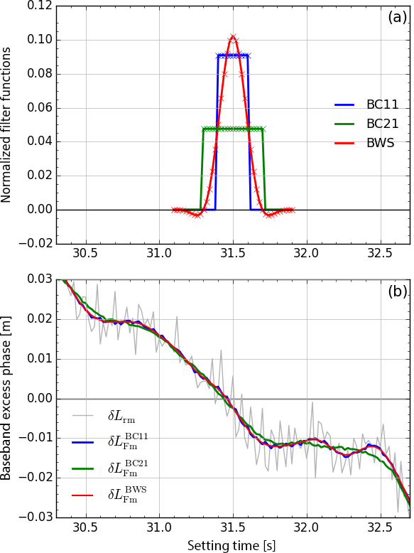
Figure A1Comparison of the Blackman windowed sinc (BWS) low-pass filter and boxcar (BC) filters based on a representative segment (between 30.3 and 32.7 s) of the excess phase profile Lr1 of the COSMIC example event. (a) Filter functions for the BWS filter with fc=2.5 Hz and M=41 points (“BWS”, red) and boxcar filters with M=21 points (“BC21”, green) and with M=11 points (“BC11”, blue), around the central value of the segment (31.5 s). (b) Filter effects on the excess phase profile Lr1 from running the filters over the segment. Shown are the unfiltered excess phase delta profile (“δLrm”, light gray), the BWS filtered profile with fc=2.5 Hz and M=41 points (“”, red), and the boxcar filtered profiles with M=21 points (“”, green) and M=11 points (“”, blue).
With such a design, the BWS low-pass filter combines efficient removal of high-frequency noise with a narrow smoothing window. The BWS filter thus achieves a better smoothing effect, while keeping a wLF of higher resolution than a simple moving-average BC filter. Based on a time segment of a few seconds of the excess phase delta profile of the COSMIC example event (also used for Figs. 3 to 8), Fig. A1 illustrates how the BWS filter compares to boxcar filters of 11 and 21 grid points. The corresponding filter functions are displayed in Fig. A1a, while Fig. A1b compares the filter results.
It is clearly seen that the smoothing window width of the BWS filter best corresponds to an 11-point boxcar filter (confirmed numerically by minimization of the sum of squared differences between boxcar and BWS filter result), while giving considerably better filtering results (as for example visible between 31.5 and 32.0 s, where the 11-point boxcar filter zigzags around the BWS result). The effective filter width of the BWS filter, which we also term “boxcar-equivalent width”, is therefore its full width at half maximum (see Fig. A1a), corresponding to samples with our design.
The actually used sample width M of the BWS filter is equal to , except that it decreases at the top and bottom of the profile such that it does not reach beyond the first/last element of the vector to be filtered. At the ith grid point (with , and N being the profile length in grid points), the filter width M is thus
The state profile of the filtered phase LF is obtained using the “baseband approach” (Kirchengast et al., 2016a), i.e., by first subtracting a zero-order model profile Lm and applying the filter only to the delta profile (with the model profile being adequately smooth over the scale of the filter window width). This approach efficiently mitigates residual numerical biases. After the application of the BWS filter, the model profile is added back again. We express the BWS filter as a linear matrix operator ABWS and get (item 1.2 in Fig. 2)
for the filtered excess phase, where . The band matrix operator ABWS has elements
The central filter weight at j=i is the (M∕2)th filter element (according to the definition of the BWS weights below); therefore its index is M∕2. With (and therefore ), each single BWS weight is calculated using
and
The estimated random uncertainty is then propagated by covariance propagation (item 1.3 in Fig. 2),
The random uncertainty profile and the error correlation matrix RLF are not needed for the subsequent random uncertainty propagation but are calculated from CLF for being available for the L1b output, using
and
The correlation length profile lLr has elements
computed upward and downward from the main peak of the correlation function and then averaged. Here dz∕dt is the scan velocity profile, obtained from using the MSL altitude grid zt calculated as part of the forward modeling towards Lm at the corresponding time grid t (cf. Table 2).
We note that after the L2a refractivity retrieval also the MSL altitude grid consistent with the retrieved refractivity profile could be used (as described by SKS2017, Appendix A therein), from a repeated forward modeling. The difference for the scan velocity estimate is found to be very small, however, since the forward-modeled zt based on collocated refractivity profiles from ECMWF short-range forecast fields is already sufficiently reliable, and this also keeps the L1b processor as a decoupled predecessor of the L2a processor.
For the estimated systematic uncertainty, interpreted as a basic systematic uncertainty (Sect. 2.2), we apply the same low-pass filter as used for the state profile (item 1.2 in Fig. 2), but with no zero-order profile subtracted, i.e.,
The resolution in time of LF and its uncertainties, τBW, is the boxcar-equivalent width (cf. Fig. A1a) determined by the cutoff frequency fc of the BWS filter,
with our design choice and with the BWS filter stopband-to-passband transition width being (Smith, 1999)
Given fc=2.5 Hz, this results in an effective resolution τLF=0.2 s and corresponds to the resolution obtained when applying a 11-point boxcar filter as explained at the beginning of this section above. The filter window intercomparison in Fig. A1a also illustrates this, because the full width at half maximum of the 2.5 Hz 41-point BWS filter is 11 points.
This resolution in time can finally be converted to the vertical (MSL altitude) resolution in space:
where, as for the correlation length estimation (Eq. A9), the scan velocity profile is employed to convert from the time domain to MSL altitude domain.
A1.2 Doppler shift derivation
After the application of the BWS filter to the excess phase profiles Lr (for both carrier frequencies of the given GNSS system), the state profile of the Doppler is derived from the filtered phase profiles LF (item 1.4 in Fig. 2). To minimize systematic errors from the numerical differentiation to negligible magnitude, the model profile Lm is again subtracted from the filtered phase profile,
and the resulting delta profile δLFm is then differentiated. After the derivative, the zero-order Doppler shift model profile Dm is added (the latter also available from the forward modeling, in a form strictly consistent with the excess phase model profile Lm).
Based on careful tests of different formulations, we use a five-point derivative scheme. The discretization of this five-point derivative δDrm,i is given by
for each of the frequencies (e.g., Syndergaard, 1999). This can be expressed in matrix form as
using matrix operator AL2D with
where , being 0.02 s in our case of fs=50 Hz.
The estimated random uncertainty can then be propagated (item 1.5 in Fig. 2) using
The covariance matrix is again (cf. Eqs. A7 and A8) decomposed into estimated random uncertainties and error correlation matrix (item 2.2 in Fig. 2) using
and
For the estimated systematic uncertainty, further on interpreted as basic systematic uncertainty (cf. Eq.A10), we apply the derivative operator (item 1.4 in Fig. 2) to the systematic uncertainties, with no zero-order profile subtracted, i.e.,
The resolution remains unaffected by the Doppler shift derivation, since the five-point sample width of the derivative operator is fully within the 11-point effective filter width (stopband) of the BWS filter applied before, so that τDr=τLF and wDr=wLF.
A2 Bending angle retrieval
A2.1 GO bending angle retrieval
From the Doppler shift state profile Dr (again for both frequencies of the given GNSS system) we can derive the impact parameter profile at and GO bending angle profile αG (item 2.1 in Fig. 2) using first the geometric relation
where
and
for each individual level of the time grid ti, in order to determine at from sequential application to all levels (Kursinski et al., 1997; Syndergaard, 1999). Here is the receiver velocity; the receiver radial position; ηR,i the angle between the receiver velocity and position vectors; ϕR,i then the angle between the receiver velocity and ray path vectors (and all these equivalently for the transmitter); and is the time derivative of the distance between the transmitter and the receiver at time ti, i.e., the “kinematic straight-line Doppler shift” to be subtracted in Eq. (A22) to match the (excess) Doppler shift Dr,i induced by the atmosphere (and ionosphere).
Based on at, the elements of the GO bending angle profile αG are subsequently calculated using another geometrical relation:
where θRT,i is the opening angle between the transmitter and receiver position vectors. Syndergaard (1999, Fig. 1.5 therein) provides an illustration of the relevant geometry.
All the variables in Eqs. (A22)–(A25) are defined in the occultation plane spanned by the receiver and transmitter position vectors after oblateness correction (Syndergaard, 1998), i.e., after they have been transformed to originate in the Earth ellipsoid's center of local curvature in the occultation plane at the mean tangent point (MTP) location of the RO event.
The MTP location is defined as the geodetic (geographic) location on the WGS84 ellipsoid, where the straight-line path between transmitter and receiver touches this ellipsoid, i.e., where the straight-line tangent height is zero. This can be computed with very high accuracy at the sub-meter level (see Scherllin-Pirscher et al., 2017, for more details on the geolocation accuracy of RO). Using the MTP location's center of local curvature rather than the Earth's center of mass as the origin is essential to ensure that the assumption of spherical symmetry, implicit in Eqs. (A22) to (A25), is accurately valid geometrically.
The impact parameter retrieval is solved iteratively, because it is impossible to rearrange Eqs. (A22) to (A24) into an explicit expression for the retrieval of the impact parameter, but it is mildly nonlinear and converges fast, in particular if the initial guess for at,i is estimated from the previous level (starting at the top level with the straight-line impact parameter).
After the GO bending angle retrieval, the bending angles of all GNSS frequencies are interpolated to a common monotonic impact altitude grid za (item 2.6 in Fig. 2), based on the monotonically sorted impact parameter grid of the leading channel, at1 (i.e., k=1).
For each element of za we get (item 2.3 in Fig. 2)
where j is the index of the elements of the sorted impact parameter grid at1. hG is the geoid undulation (see Scherllin-Pirscher et al., 2017, for a detailed discussion of its use in RO analysis), and RC is the local radius of curvature of the RO event.
Because the impact parameter is only implicitly expressed in Eqs. (A22)–(A24), but GUM-type uncertainty propagation along Eqs. (2) and (4) requires an explicit measurement model, we make use of a linearization of the bending angle retrieval. We use the approach described by Melbourne et al. (1994), and applied to uncertainty propagation by Syndergaard (1999), for the propagation of the estimated random uncertainty from Doppler shift Dr to GO bending angle αG (item 2.5 in Fig. 2).
This linearization establishes a direct relation between random uncertainties of the Doppler shift and the uncertainties of the bending angle , using
where aSL is the straight-line impact parameter. These bending angle uncertainties are relative to the time grid as independent coordinate. To get the desired uncertainties with respect to the impact altitude grid za (introduced in Eq. A26), the uncertainties of the impact altitude za need to be transferred to the bending angle, so that the za grid can subsequently be considered free of error. Syndergaard (1999) showed that this can be done by replacing Eq. (A27) with
where is the “true” impact parameter. We use the forward-modeled impact parameter atm instead (i.e., adopt ) and accept the additional error thus incurred, assuming it is smaller than the 2 % relative error due to the linearization estimated by Melbourne et al. (1994). This is a reasonable assumption given the high quality of our forward-modeled profiles derived from ECMWF short-range forecast refractivity fields.
As a consequence we have to accept that the overall inaccuracy of our random uncertainty estimate cannot be brought below 2 %. Therefore, to ensure that our simplified estimate does not underestimate the real uncertainty, we account for the linearization error by multiplying a factor fuαlin=1.02 to the uncertainty of the retrieved GO bending angle
In this way we acknowledge that although the calculation of the state of the bending angle does not make use of the linearization, and therefore the linearization does not increase the uncertainty of the state profile, it may increase the error in the uncertainty estimate itself.
Finally, the profile is also interpolated to the common monotonic impact altitude grid za.
In the GO approximation, the bending angle values at each grid point only depend on the Doppler shift values of the same grid points; i.e., the existing correlations between the errors at different levels are left unchanged: i.e., RαG=RDr. The covariance matrix can hence be calculated by recombining the Doppler shift correlation matrix with the propagated uncertainties (item 2.8 in Fig. 2),
For the propagation of the estimated systematic uncertainty (item 2.4 in Fig. 2) three types of potential systematic errors adding to the impact parameter uncertainty , and consequentially the bending angle uncertainty , are taken into account: systematic errors in the Doppler shift, i.e., ; systematic errors in the velocities of the satellites, i.e., and ; and systematic errors in the positions of the satellites, i.e., and . The latter two orbit-borne types are interpreted as apparent systematic uncertainties (Sect. 2.2), while the excess phase-borne uncertainty is a basic systematic uncertainty.
For the propagation of these estimated systematic uncertainties to , Eqs. (A22)–(A24) are linearized around the retrieved state quantities (serving as zero-order state), and no terms higher than first-order are kept. Then ϕR and ϕT in Eq. (A22) are substituted by the linearized versions of Eqs. (A23) and (A24), and the resulting equation is solved (level by level) for the impact parameter , with . Adopting the first-order deviations to represent the estimated systematic uncertainties, we obtain
where
A number of simplifications have been made to arrive at this result. First, the last term in Eq. A22 is disregarded since errors in the positions are assumed to be constant with respect to the short time duration of an RO event; remaining errors after taking the derivative are therefore of higher order. Next, orbit position and velocity uncertainties are both assumed to be constant within the short duration of an event, and the velocity uncertainties obtained are interpreted as uncertainties along the direction of the velocity vector. Consequentially, the uncertainty is also projected along with the vector into the ray path direction. A more conservative estimation (which we consider overly conservative in context) would interpret the uncertainties as ellipsoids at the velocity vectors' heads and would hence take the full magnitude of the uncertainties along the ray path direction (without projection).
Furthermore, since all error sources (the processing of the occultation tracking data and the POD for transmitter and receiver) are essentially independent from each other, the different input uncertainties are assumed to be uncorrelated. Finally, we reasonably assumed the errors of the angle between the position and velocity vectors (η) to be negligible () for the purpose here, for both the transmitter and receiver.
In order to finally derive the systematic uncertainty of the bending angle from the impact parameter's uncertainty, we continue with a linearization of Eq. (A25) and arrive at
where
In practice we separately calculate the basic and apparent systematic uncertainty estimates ( from the first RHS terms in Eqs. A31 and A33, from the orbit-borne terms) and afterwards obtain as a combined result, in order to enable separate propagation in subsequent processing steps.
The resolution profile remains unaffected by the bending angle retrieval, since the level-by-level approach of the algorithm does not create extra correlation and further vertical smoothing, so that ταG=τDr and wαG=wDr.
A2.2 WO bending angle retrieval
After the GO bending angle, the WO bending angle state profile αW(za) is retrieved (item 2.7 in Fig. 2) from excess phase profile Lr(t) (and its uncertainties) and the amplitude profile Ar(t) (and uncertainties) in a WO retrieval following Gorbunov and Kirchengast (2015, 2018). Along with the state profile, the systematic uncertainty profile , the covariance matrix CαW, and the resolution profile wαW are derived.
The covariance matrix CαW is then decomposed to random uncertainty profile and correlation matrix RαW in the same form as done above for CDr (Eqs. A19 and A20) and CLF (Eqs. A7 and A8). The estimated systematic uncertainty is composed of a basic systematic uncertainty , propagated through the wave-optical retrieval from the excess phase uncertainty , and an apparent systematic uncertainty , estimated in the lower troposphere as residual bias uncertainty of a regression-based boundary layer bias correction (Gorbunov and Kirchengast, 2018).
The WO bending angle retrieval algorithm and the associated uncertainty propagation algorithm are not explicitly described here; the reader is referred to Gorbunov and Kirchengast (2015) and Gorbunov and Kirchengast (2018). However, we have prepared the merging with the WO bending angle variables (they will be actually merged in when the WO tests within the rOPS are complete), which is described next.
A2.3 Merging of GO and WO bending angle profiles
The αW profile, prepared on the common grid za, and the αG profile are merged over an upper-tropospheric transition range (item 2.9 in Fig. 2). The gradual transition, weighted by a symmetric half-sine function, has a defined impact altitude transition of half-width km around transition altitude , allowed within 9 km to 14 km, estimated from αG data quality. The resulting merged bending angle profile αM is
where the weighting profile γ is formulated as
To determine the random uncertainties for the merged GO–WO input bending angle, we need to merge the covariance matrices of both bending angles.
We can assume both incoming covariance matrices CαG and CαW are provided on the common monotonic target grid za (i.e., also the WO uncertainties and correlations are interpolated to this common grid before the merger). We further can reasonably assume that there are no cross-correlations between GO and WO errors, given the very different retrieval schemes. Based on this we can compose the covariance matrix of the merged bending angle profile, CαM (item 2.10 in Fig. 2) as follows. Outside the merging zone (i.e., outside of ) we can assign
while within the merging zone we can assign
wherein i is understood such that and j such that .
Because of the symmetry of the covariance matrix, the covariance elements in the merging zone orthogonal to the one above, i.e., for and , are calculated according to the same formula.
Due to the linear relation between αM, αG, and αW, expressed by Eq. (A35), a bias in the GO bending angle and a bias in the WO bending angle can be combined linearily as well, and we can compute the estimated systematic uncertainty of the merged bending angle according to (item 2.9 in Fig. 2)
In practice this formulation is again applied separately for the basic and apparent systematic uncertainty estimates, afterwards obtaining the profile as a combined result, in order to allow separate propagation in subsequent processing steps.
The resolution profile of the bending angle, wαM, is equal to the GO resolution wαG above , equal to the WO resolution wαW below and has a transition with transition weight γi in between, again following the linear formulation such as in Eqs. (A35) and (A39).
Because the integration and testing of the uncertainty propagation through the rOPS WO bending angle retrieval are currently still ongoing, as noted in Sect. A2.2 above, the examples shown in this study are all GO-only; i.e., only the GO retrieval is performed. The merging algorithm as described is ready to include the WO bending angles, however.
A3 Atmospheric bending angle derivation
In order to retrieve the atmospheric bending angle profile αr, ionospheric effects need to be corrected for, using the retrieved bending angles from each transmitter frequency channel. Since the only GNSS constellation currently used for RO is the GPS – except for recent initial data from the Chinese GNOS instrument using BeiDou signals (Liao et al., 2016; Bai et al., 2018) – the data characteristics of the GPS case (with , fT1=1.57542 GHz, and fT2=1.22760 GHz) are in the prime focus of this section.
This concerns in particular special provisions for the minor (L2) channel noise filtering and its tropospheric extrapolation. In general the algorithms are applicable for any of the available GNSS systems, however; if the minor channel (fT2) delivers similar data quality to the major one (fT1), the special provisions for the former will practically have no effect.
A3.1 Adaptive low-pass filtering and minor-channel extrapolation
Before applying the dual-frequency ionospheric correction, the merged bending angle state profiles αM,k(za) at the common za grid are filtered with further BWS low-pass filter operations, and the minor channel is extrapolated.
For αM1 the filter is set to the same cutoff frequency as the basic BWS filter preceding the Doppler derivation (i.e., fc1=2.5 Hz), ensuring a reliable reference resolution and basic smoothness of the whole merged profile. For filtering of αM2 a (GPS L2) noise-minimization algorithm is used, following the approach of Sokolovskiy et al. (2009) for optimal filtering for ionospheric correction. We search for minimized noise employing a flexible cutoff frequency fc2∈{2.5, 2, 10∕7, 1, 5∕7, 0.5 Hz}, corresponding to using cutoff periods τc2 from 0.4 to 2 s and sample widths of M=40 to M=200 (for BWS filter design details see Sect. A1.1).
We adopt the cutoff frequency fc2 for αM2 filtering that minimizes the noise fluctuations of the ionosphere-corrected atmospheric bending angle delta profile when evaluated over the mesospheric altitude range between 50 and 70 km (similar to the functional minimization of Sokolovskiy et al., 2009; Eq. 4 therein). At these high altitudes the residual atmospheric mean signal after subtraction of the forward-modeled signal αm(za) is very small (< 0.03–0.3 µrad), and therefore the noise level representative for the given RO event is well quantifiable.
The weight matrix of the BWS filter, , is determined for both frequencies analogously to Eqs. (A3) to (A5). When using the baseband approach with model profile αm to create the delta profile δαMm with elements
the filtered bending angle is then (item 3.1 in Fig. 2)
where and .
Due to the stronger power of the L1 signal for (most of) the GPS satellites, the GPS signals of both frequencies are not of the same quality, and the L2 data (for those satellites where encrypted and hence power-degraded L2 signals are transmitted) do not reach down as far as the L1 data (i.e., zaBot2>zaBot1). If due to this reason αF2 does not reach down as far as αF1 and zaBot2≤zaBot2Max (with zaBot2Max currently set to 15 km), a tropospheric bending angle extrapolation (TBAE) is applied in order to artificially extend αM2 to also reach down to zaBot1 (item 3.3 in Fig. 2).
Briefly summarized, this TBAE is currently implemented as follows. A linear gradient profile for the difference profile between the two bending angles, , is estimated by a least squares fit over a sufficiently wide impact altitude range from zaBot2 upward (as wide as the extrapolation range, at least 10 km). This gradient profile is then linearly extended down to zaBot1 and subtracted from αF1, to obtain the extrapolated part of αF2 from zaBot2 to zaBot1. If zaBot2>zaBot2Max, then no TBAE is performed since the extrapolation range is considered too large. Details are provided by Kirchengast et al. (2017b), where the most recent version of the atmospheric bending angle derivation is described that includes this αF12 extrapolation in a further advanced form.
For the propagation of the estimated random uncertainty we get (item 3.2 in Fig. 2)
for the bending angle error covariance matrices of the leading (k=1) and minor (k=2) channel.
If a TBAE is applied to αF2, the random uncertainty of αF2 below zaBot2 is equal to that of αF1, because the noise is “copied” from αF1 since the linear gradient profile from fitting αF12 is noise-free. As a consequence, in these cases, we set the matrix elements of CαF2 to (item 3.4 in Fig. 2)
CαF1 and CαF2 can then be decomposed as needed into , RαF1, and , RαF2, respectively. Kirchengast et al. (2017b) describe the most recent version consistent with a further advanced form of the TBAE, where the separate assignments according to Eq. (A43) are no longer needed.
The estimated systematic uncertainties (in practice the basic and apparent systematic uncertainty estimates separately) are filtered with the same filter settings as for the state profiles (item 3.1 in Fig. 2) and are thus obtained in the form
Since these are smooth profiles, they are marginally changed by this low-pass filtering. The systematic uncertainty component contributed by the TBAE to the estimated systematic uncertainty is added after the ionospheric correction (see next subsection).
As for the basic low-pass filtering of excess phases (Sect. A1.1), the resolution profiles of the filtered bending angles wαF1 and wαF2 are determined by the cutoff frequencies fc1 and fc2 of the BWS filters, following Eqs. (A11) and (A13).
A3.2 Ionospheric correction
Based on the filtered and sometimes extrapolated state profiles αF1 and αF2, the ionospheric refractive effects are corrected for by the standard dual-frequency correction of bending angles (Vorob'ev and Krasil'nikova, 1994) used in the fT1–fT2 difference profile form (Sokolovskiy et al., 2009) (item 3.5 in Fig. 2). For the elements of the retrieved atmospheric bending angle profile αr we thus get
where
and
Propagated through the operator of the ionospheric correction (Eq. A45, currently used here in the classical form with fT1 and fT2 terms), the estimated random uncertainty of the resulting atmospheric bending angle, expressed by the error covariance matrix Cαr (item 3.6 in Fig. 2), is obtained as
Cαr can then also be decomposed into and Rαr with the usual equations (cf., e.g., Eqs. A19 and A20).
Equation (A45) is as well applied to propagate the estimated systematic uncertainty (in practice the basic and apparent systematic uncertainty estimates separately) through the ionospheric correction using (item 3.5 in Fig. 2)
where it is assumed that the systematic errors in αF1 and αF2 are positively correlated, i.e., have the same sign, and the associated uncertainty estimates are hence subtracted from one another (as the bending angles are in Eq. A46). This assumption is reasonable, since the same sources of non-ionospheric systematic effects apply to both frequency channels (Doppler shift, orbit velocity, and orbit position uncertainties).
In the case of TBAE, Eq. (A49) needs to be supplemented below zaBot2, since additional uncertainties arise from the errors made in the fitting parameters and in the extrapolation model (linear extrapolation) of the TBAE. Hence, for the range ,
with being the conservative estimate for additional (apparent) systematic uncertainty within the extrapolated impact altitude range. We set to zero at zaBot2 and linearly increase it from there downwards with a gradient of 1 µrad per 10 km (an experience-based best guess; cf. Scherllin-Pirscher et al., 2011b, a, who also address aspects of such tropospheric extrapolation in their discussions of error sources). It is interpreted as an apparent systematic uncertainty estimate, since due to the linear fit-based TBAE construction its event-to-event bias character will be essentially random (Scherllin-Pirscher et al., 2011b).
Also, the ionospheric correction currently applied in the rOPS is just a first-order correction, which will leave higher-order residual ionospheric errors in αr (e.g., Syndergaard, 2000; Danzer et al., 2013; Liu et al., 2013, 2015; Healy and Culverwell, 2015). The uncertainty from higher-order residual ionospheric biases (RIBs), , is therefore added to the propagated (basic) systematic uncertainty. is interpreted as basic systematic uncertainty, since the higher-order ionospheric residuals may not vanish in ensemble-of-events averaging. The other non-ionospheric sources of systematic errors and the RIBs can be reasonably assumed to be uncorrelated. The total estimated systematic uncertainty of the retrieved atmospheric bending angle αr hence is
Based on previous studies (e.g., Liu et al., 2013, 2015; Danzer et al., 2013, 2015), is taken to be constant along the entire profile and is estimated to amount to 0.05 µrad. These last two components, and , are indicated as item 3.7 in Fig. 2. It is clear that this initial systematic uncertainty estimation can be significantly improved by future dedicated work on better quantifying and (if suitable) correcting for the systematic uncertainty components.
The resolution of the retrieved bending angle, wαr, essentially corresponds to the higher resolution of the two bending angle profiles αF1 and αF2, and thus generally closely matches wαF1 in most cases. As a simple but robust and suitable estimate, assuming that the resolutions of αr and αF1 scale in the same way as the correlation lengths lαr and lαF1 (derived from Rαr and RαF1 as described for RLF in Eq. A9), we compute wαr as
In concluding, we note that the atmospheric bending angle derivation algorithms used in this study – i.e., the adaptive filtering, TBAE, and ionospheric correction parts as described in this section – have recently received further advancement towards a form fully based on the combination of αF1 and the difference profile αF12 (rather than of αF1 and αF2), more aligned with the concept of Sokolovskiy et al. (2009). A detailed description of this most recent version is found in Kirchengast et al. (2017b).
The full covariance propagation applied to propagate random uncertainties requires numerically “expensive” matrix operations, and therefore considerable efforts were made to seize opportunities for reducing the number of numerical operations (e.g., by only calculating with those elements of the band matrix ABWS which lie within the width of the filter window).
However, as demonstrated in Sect. 4, simplification to a mere variance propagation (i.e., only considering the diagonal elements of the covariance matrices) is not reasonably possible because it leads to an unacceptable overestimation of random uncertainties. This overestimation occurs since the influence of the covariance elements – and thus for example the partially compensating impact of the negative side peaks in the correlation functions – is disregarded.
Here we state the two equations used to obtain the variances-only propagation results shown for comparison purposes in Fig. 9: the estimated random uncertainty was propagated through the BWS filter using
and subsequently through the ionospheric correction using
JS and GK designed the study, including comments by MS, based on the concept and framework of uncertainty propagation into the Reference Occultation Processing system (rOPS), formulated by GK. JS elaborated the detailed algorithms, performed the computational implementation and the analysis, prepared the figures, and wrote the first draft of the paper; he was advised and supported in this work by GK and MS. As part of this support GK provided detailed design input and feedback and substantially contributed to the writing of the paper, and MS substantially contributed to the computational work. Based on a primary role of the first two authors, all authors contributed to consolidating the paper for submission and towards publication.
The authors declare that they have no conflict of interest.
This article is part of the special issue “Observing Atmosphere and Climate with Occultation Techniques – Results from the OPAC-IROWG 2016 Workshop”. It is a result of the International Workshop on Occultations for Probing Atmosphere and Climate, Leibnitz, Austria, 8–14 September 2016.
We thank UCAR/CDAAC Boulder for access to their RO excess phase and
orbit data as well as ECMWF Reading for access to their analysis and forecast
data. The work was funded by the Austrian Aeronautics and Space Agency of the
Austrian Research Promotion Agency (FFG-ALR) under projects
OPSCLIMPROP and OPSCLIMTRACE and by the European Space Agency
(ESA) under project MMValRO-E.
Edited by: Sean Healy
Reviewed by: two anonymous referees
Angerer, B., Ladstädter, F., Scherllin-Pirscher, B., Schwärz, M., Steiner, A. K., Foelsche, U., and Kirchengast, G.: Quality aspects of the Wegener Center multi-satellite GPS radio occultation record OPSv5.6, Atmos. Meas. Tech., 10, 4845–4863, https://doi.org/10.5194/amt-10-4845-2017, 2017. a
Anthes, R. A.: Exploring Earth's atmosphere with radio occultation: contributions to weather, climate and space weather, Atmos. Meas. Tech., 4, 1077–1103, https://doi.org/10.5194/amt-4-1077-2011, 2011. a
Anthes, R. A., Bernhardt, P. A., Chen, Y., Cucurull, L., Dymond, K. F., Ector, D., Healy, S. B., Ho, S.-P., Hunt, D. C., Kuo, Y.-H., Liu, H., Manning, K., McCormick, C., Meehan, T. K., Randel, W. J., Rocken, C., Schreiner, W. S., Sokolovskiy, S. V., Syndergaard, S., Thompson, D. C., Trenberth, K. E., Wee, T.-K., Yen, N. L., and Zeng, Z.: The COSMIC/FORMOSAT-3 mission: Early results, B. Am. Meteorol. Soc., 89, 313–333, https://doi.org/10.1175/BAMS-89-3-313, 2008. a
Bai, W., Liu, C., Meng, X., Sun, Y., Kirchengast, G., Du, Q., Wang, X., Yang, G., Liao, M., Yang, Z., Zhao, D., Xia, J., Cai, Y., Liu, L., and Wang, D.: Evaluation of atmospheric profiles derived from single- and zero-difference excess phase processing of BeiDou radio occultation data from the FY-3C GNOS mission, Atmos. Meas. Tech., 11, 819–833, https://doi.org/10.5194/amt-11-819-2018, 2018. a
Bauer, P., Andersson, E., and Richardson, D.: The quiet revolution of numerical weather prediction, Nature, 525, 47–55, https://doi.org/10.1038/nature14956, 2015. a
Bojinski, S., Verstraete, M., Peterson, T. C., Richter, C., Simmons, A., and Zemp, M.: The concept of Essential Climate Variables in support of climate research, applications, and policy, B. Am. Meteorol. Soc., 95, 1431–1443, https://doi.org/10.1175/BAMS-D-13-00047.1, 2014. a
Danzer, J., Scherllin-Pirscher, B., and Foelsche, U.: Systematic residual ionospheric errors in radio occultation data and a potential way to minimize them, Atmos. Meas. Tech., 6, 2169–2179, https://doi.org/10.5194/amt-6-2169-2013, 2013. a, b, c, d
Danzer, J., Healy, S. B., and Culverwell, I. D.: A simulation study with a new residual ionospheric error model for GPS radio occultation climatologies, Atmos. Meas. Tech., 8, 3395–3404, https://doi.org/10.5194/amt-8-3395-2015, 2015. a, b, c
ESA/EUMETSAT: The GRAS instrument on METOP, ESA/EUMETSAT rep. esa vr/3021/pi, eumetsat eps/mis/in/9, ESA, Noordwijk, the Netherlands, 1998. a, b
Fritzer, J., Kirchengast, G., and Pock, M.: EGOPS 5.5/SUM, End-to-End Generic Occultation Performance Simulation and Processing System, Version 5.5, Software User Manual, WEGC-IGAM/Uni Graz technical report for ESA/ESTEC No. 1/2009, Doc-Id: WEGC–EGOPS–2009–TR01, WEGC and IGAM, University of Graz, Graz, Austria, 2009. a
GCOS: Guideline for the Generation of Datasets and Products Meeting GCOS Requirements, WMO-TD/No. 1530, WMO, Geneva, GCOS-143, update to GCOS-128, available at: http://www.wmo.int/pages/prog/gcos/Publications/gcos-143.pdf (last access: 20 November 2017), 2010. a
GCOS: Status of the Global Observing System for Climate – Full Report, GCOS-195, WMO, Geneva, available at: http://www.wmo.int/pages/prog/gcos/Publications/GCOS-195_en.pdf (last access: 20 November 2017), 2015. a, b
Gorbunov, M. E.: Canonical transform method for processing radio occultation data in the lower troposphere, Radio Sci., 37, 1076, https://doi.org/10.1029/2000RS002592, 2002a. a
Gorbunov, M. E.: Ionospheric correction and statistical optimization of radio occultation data, Radio Sci., 37, 1084, https://doi.org/10.1029/2000RS002370, 2002b. a
Gorbunov, M. E. and Kirchengast, G.: Uncertainty propagation through wave optics retrieval of bending angles from GPS radio occultation: Theory and simulation results, Radio Sci., 50, RS6001, https://doi.org/10.1002/2015RS005730, 2015. a, b, c, d
Gorbunov, M. E. and Kirchengast, G.: Wave-optics uncertainty propagation and regression-based bias model in GNSS radio occultation bending angle retrievals, Atmos. Meas. Tech., 11, 111–125, https://doi.org/10.5194/amt-11-111-2018, 2018. a, b, c, d, e, f, g
Gorbunov, M. E. and Lauritsen, K. B.: Analysis of wave fields by Fourier integral operators and their application for radio occultations, Radio Sci., 39, RS4010, https://doi.org/10.1029/2003RS002971, 2004. a
Gorbunov, M. E., Benzon, H.-H., Jensen, A. S., Lohmann, M. S., and Nielsen, A. S.: Comparative analysis of radio occultation processing approaches based on Fourier integral operators, Radio Sci., 39, RS6004, https://doi.org/10.1029/2003RS002916, 2004. a, b
Hajj, G. A., Kursinski, E. R., Romans, L. J., Bertiger, W. I., and Leroy, S. S.: A technical description of atmospheric sounding by GPS occultation, J. Atmos. Sol.-Terr. Phy., 64, 451–469, https://doi.org/10.1016/S1364-6826(01)00114-6, 2002. a, b
Healy, S. B. and Culverwell, I. D.: A modification to the standard ionospheric correction method used in GPS radio occultation, Atmos. Meas. Tech., 8, 3385–3393, https://doi.org/10.5194/amt-8-3385-2015, 2015. a, b
Ho, S.-P., Hunt, D., Steiner, A. K., Mannucci, A. J., Kirchengast, G., Gleisner, H., Heise, S., von Engeln, A., Marquardt, C., Sokolovskiy, S., Schreiner, W., Scherllin-Pirscher, B., Ao, C., Wickert, J., Syndergaard, S., Lauritsen, K., Leroy, S., Kursinski, E. R., Kuo, Y.-H., Foelsche, U., Schmidt, T., and Gorbunov, M.: Reproducibility of GPS radio occultation data for climate monitoring: Profile-to-profile inter-comparison of CHAMP climate records 2002 to 2008 from six data centers, J. Geophys. Res., 117, D18111, https://doi.org/10.1029/2012JD017665, 2012. a, b
Innerkofler, J., Pock, C., Kirchengast, G., Schwärz, M., Jäggi, A., Andres, Y., Marquardt, C., and Schwarz, J.: GNSS radio occultation zero-differencing excess phase processing with integrated uncertainty estimation for climate applications, presentation at COSMIC-IROWG International Workshop, 21–27 September 2017, Estes Park, Colorado USA, available at: https://cpaess.ucar.edu/sites/default/files/meetings/2017/cosmic/posters/innerkofler-josef-poster.pdf (last access: 23 April 2018), 2017. a, b, c, d, e
JCGM: Evaluation of Measurement Data – Guide to the Expression of Uncertainty in Measurement, Rep. JCGM 100:2008, Joint Committee for Guides in Metrology, Office BIPM, Paris, France, 2008a. a
JCGM: Evaluation of Measurement Data – Supplement 1 to the “Guide to the Expression of Uncertainty in Measurement” – Propagation of distributions using a Monte Carlo method, Rep. JCGM 101:2008, Joint Committee for Guides in Metrology, Office BIPM, Paris, France, 2008b. a
JCGM: Evaluation of Measurement Data – Supplement 2 to the “Guide to the Expression of Uncertainty in Measurement” – Extension to any number of output quantities, Rep. JCGM 102:2011, Joint Committee for Guides in Metrology, Office BIPM, Paris, France, 2011. a, b
JCGM: International Vocabulary of Metrology – Basic and General Concepts and Associated Terms (VIM 3rd edition), Rep. JCGM 200:2012, Joint Committee for Guides in Metrology, Office BIPM, Paris, France, 2012. a
Karl, T. R., Derr, V. E., Easterling, D. R., Folland, C. K., Hofmann, D. J., Levitus, S., Nicholls, N., Parker, D. E., and Withee, G. W.: Critical issues for long-term climate monitoring, Clim. Change, 31, 185–221, https://doi.org/10.1007/BF01095146, 1995. a
Kirchengast, G., Schwärz, M., Schwarz, J., Scherllin-Pirscher, B., Pock, C., and Innerkofler, J.: Reference Occultation Processing System (rOPS) for cal/val and climate: a new GNSS RO retrieval chain with integrated uncertainty propagation, Presentation at the IROWG-4 international workshop, 16–22 April 2015, Bureau of Meteorology, Melbourne, Australia, available at: http://irowg.org/wpcms/wp-content/uploads/2014/05/Kirchengast-IROWG-4.pdf (last access: 20 November 2017), 2015. a
Kirchengast, G., Schwärz, M., Schwarz, J., Scherllin-Pirscher, B., Pock, C., Innerkofler, J., Proschek, V., Steiner, A. K., Danzer, J., Ladstädter, F., and Foelsche, U.: Employing GNSS radio occultation for solving the global climate monitoring problem for the fundamental state of the atmosphere, Presentation at the EGU 2016 General Assembly, 17–22 April 2016, Vienna, Austria, Geophys. Res. Abstracts, 18, EGU2016-12035-1, available at: http://meetingorganizer.copernicus.org/EGU2016/EGU2016-12035-1.pdf (last access: 20 November 2017), 2016a. a, b, c, d
Kirchengast, G., Schwärz, M., Schwarz, J., Scherllin-Pirscher, B., Pock, C., Innerkofler, J., Proschek, V., Steiner, A. K., Danzer, J., Ladstädter, F., and Foelsche, U.: The reference occultation processing system approach to interpret GNSS radio occultation as SI-traceable planetary system refractometer, presentation at OPAC-IROWG International Workshop 8–14 September 2016, Seggau/Leibnitz, Austria, available at: http://wegcwww.uni-graz.at/opacirowg2016/data/public/files/opacirowg2016_Gottfried_Kirchengast_presentation_261.pdf (last access: 20 November 2017), 2016b. a, b
Kirchengast, G., Li, Y., Scherllin-Pirscher, B., Schwärz, M., Schwarz, J., and Nielsen, J. K.: A new retrieval algorithm for tropospheric temperature, humidity and pressure profiling based on GNSS radio occultation data, Presentation at the EGU 2017 General Assembly, 23–28 April 2017, Vienna, Austria, Geophys. Res. Abstracts, 19, EGU2017-16328-2 available online at http://meetingorganizer.copernicus.org/EGU2017/EGU2017-16328-2.pdf (last access: 23 April 2018), 2017a. a
Kirchengast, G., Schwärz, M., Schwarz, J., Ramsauer, J., Fritzer, J., Scherllin-Pirscher, B., Innerkofler, J., Proschek, V., Rieckh, T., and Danzer, J.: Reference OPS DAD – Reference Occultation Processing System (rOPS) Detailed Algorithm Description, Tech. Rep. for ESA and FFG No. 1/2017, Doc-Id: WEGC–rOPS–2017–TR01, Issue 1.7, Wegener Center, Univ. of Graz, Graz, Austria, 2017b. a, b, c, d
Kuo, Y.-H., Wee, T.-K., Sokolovskiy, S., Rocken, C., Schreiner, W., Hunt, D., and Anthes, R. A.: Inversion and error estimation of GPS radio occultation data, J. R. Stat. Soc., 82, 507–531, 2004. a
Kursinski, E. R., Hajj, G. A., Schofield, J. T., Linfield, R. P., and Hardy, K. R.: Observing Earth's atmosphere with radio occultation measurements using the Global Positioning System, J. Geophys. Res., 102, 23429–23465, https://doi.org/10.1029/97JD01569, 1997. a, b, c, d, e
Leroy, S. S., Dykema, J. A., and Anderson, J. G.: Climate benchmarking using GNSS occultation, in: Atmosphere and Climate: Studies by Occultation Methods, edited by: Foelsche, U., Kirchengast, G., and Steiner, A. K., 287–301, Springer, Berlin Heidelberg, Germany, 2006. a
Li, Y., Kirchengast, G., Scherllin-Pirscher, B., Wu, S., Schwaerz, M., Fritzer, J., Zhang, S., Carter, B. A., and Zhang, K.: A new dynamic approach for statistical optimization of GNSS radio occultation bending angles for optimal climate monitoring utility, J. Geophys. Res.-Atmos., 118, 13022–13040, https://doi.org/10.1002/2013JD020763, 2013. a
Li, Y., Kirchengast, G., Scherllin-Pirscher, B., Norman, R., Yuan, Y. B., Fritzer, J., Schwaerz, M., and Zhang, K.: Dynamic statistical optimization of GNSS radio occultation bending angles: advanced algorithm and performance analysis, Atmos. Meas. Tech., 8, 3447–3465, https://doi.org/10.5194/amt-8-3447-2015, 2015. a, b
Li, Y., Kirchengast, G., Scherllin-Pirscher, B., Schwärz, M., Nielsen, J. K., Wee, T.-K., Ho, S.-P., and Yuan, Y.-B.: A new algorithm for the retrieval of atmospheric profiles from GNSS radio occultation data in moist air and cross-evaluation among processing centers, J. Geophys. Res.-Atmos, submitted, 2018. a
Liao, M., Zhang, P., Yang, G.-L., Bi, Y.-M., Liu, Y., Bai, W.-H., Meng, X.-G., Du, Q.-F., and Sun, Y.-Q.: Preliminary validation of the refractivity from the new radio occultation sounder GNOS/FY-3C, Atmos. Meas. Tech., 9, 781–792, https://doi.org/10.5194/amt-9-781-2016, 2016. a
Liu, C.-L., Kirchengast, G., Zhang, K., Norman, R., Li, Y., Zhang, S. C., Carter, B., Fritzer, J., Schwaerz, M., Choy, S. L., Wu, S. Q., and Tan, Z. X.: Characterisation of residual ionospheric errors in bending angles using GNSS RO end-to-end simulations, Adv. Space Res., 52, 821–836, https://doi.org/10.1016/j.asr.2013.05.021, 2013. a, b
Liu, C. L., Kirchengast, G., Zhang, K., Norman, R., Li, Y., Zhang, S. C., Fritzer, J., Schwaerz, M., Wu, S. Q., and Tan, Z. X.: Quantifying residual ionospheric errors in GNSS radio occultation bending angles based on ensembles of profiles from end-to-end simulations, Atmos. Meas. Tech., 8, 2999–3019, https://doi.org/10.5194/amt-8-2999-2015, 2015. a, b, c, d
Luntama, J.-P., Kirchengast, G., Borsche, M., Foelsche, U., Steiner, A., Healy, S. B., von Engeln, A., O'Clerigh, E., and Marquardt, C.: Prospects of the EPS GRAS mission for operational atmospheric applications, B. Am. Meteorol. Soc., 89, 1863–1875, https://doi.org/10.1175/2008BAMS2399.1, 2008. a, b, c
Melbourne, W. G., Davis, E. S., Duncan, C. B., Hajj, G. A., Hardy, K. R., Kursinski, E. R., Meehan, T. K., Young, L. E., and Yunck, T. P.: The application of spaceborne GPS to atmospheric limb sounding and global change monitoring, JPL Publication, Pasadena, USA, 94–18, 1994. a, b
Montenbruck, O., Garcia-Fernandez, M., Yoon, Y., Schön, S., and Jäggi, A.: Antenna phase center calibration for precise positioning of LEO satellites, GPS Solut., 13, 23–34, https://doi.org/10.1007/s10291-008-0094-z, 2009. a
NRC: Earth Science and Applications from Space: National Imperatives for the Next Decade and Beyond (Decadal Survey), The National Academies Press, Washington, D.C., https://doi.org/10.17226/11820, 2007. a
Rieder, M. J. and Kirchengast, G.: Error analysis and characterization of atmospheric profiles retrieved from GNSS occultation data, J. Geophys. Res., 106, 31755–31770, 2001. a
Scherllin-Pirscher, B., Kirchengast, G., Steiner, A. K., Kuo, Y.-H., and Foelsche, U.: Quantifying uncertainty in climatological fields from GPS radio occultation: an empirical-analytical error model, Atmos. Meas. Tech., 4, 2019–2034, https://doi.org/10.5194/amt-4-2019-2011, 2011a. a, b
Scherllin-Pirscher, B., Steiner, A. K., Kirchengast, G., Kuo, Y.-H., and Foelsche, U.: Empirical analysis and modeling of errors of atmospheric profiles from GPS radio occultation, Atmos. Meas. Tech., 4, 1875–1890, https://doi.org/10.5194/amt-4-1875-2011, 2011b. a, b, c
Scherllin-Pirscher, B., Steiner, A. K., Kirchengast, G., Schwaerz, M., and Leroy, S. S.: The power of vertical geolocation of atmospheric profiles from GNSS radio occultation, J. Geophys. Res.-Atmos., 122, 1595–1616, https://doi.org/10.1002/2016JD025902, 2017. a, b, c
Schreiner, W. S., Rocken, C., Sokolovskiy, S., and Hunt, D.: Quality assessment of COSMIC/FORMOSAT-3 GPS radio occultation data derived from single- and double-difference atmospheric excess phase processing, GPS Solut., 14, 13–22, https://doi.org/10.1007/s10291-009-0132-5, 2010. a
Schwarz, J. C., Kirchengast, G., and Schwaerz, M.: Integrating uncertainty propagation in GNSS radio occultation retrieval: from bending angle to dry-air atmospheric profiles, Earth Space Sci., 4, 200–228, https://doi.org/10.1002/2016EA000234, 2017. a, b
Smith, S. W.: The Scientist and Engineer's Guide to Digital Signal Processing, California Technical Publishing, 2nd Edn., San Diego, USA, 1999. a, b
Sokolovskiy, S. V., Schreiner, W. S., Rocken, C., and Hunt, D.: Optimal noise filtering for the ionospheric correction of GPS radio occultation signals, J. Atmos. Ocean. Tech., 26, 1398–1403, https://doi.org/10.1175/2009JTECHA1192.1, 2009. a, b, c, d, e
Steiner, A. K. and Kirchengast, G.: Error analysis of GNSS radio occultation data based on ensembles of profiles from end-to-end simulations, J. Geophys. Res., 110, D15307, https://doi.org/10.1029/2004JD005251, 2005. a
Steiner, A. K., Lackner, B. C., Ladstädter, F., Scherllin-Pirscher, B., Foelsche, U., and Kirchengast, G.: GPS radio occultation for climate monitoring and change detection, Radio Sci., 46, RS0D24, https://doi.org/10.1029/2010RS004614, 2011. a
Steiner, A. K., Hunt, D., Ho, S.-P., Kirchengast, G., Mannucci, A. J., Scherllin-Pirscher, B., Gleisner, H., von Engeln, A., Schmidt, T., Ao, C., Leroy, S. S., Kursinski, E. R., Foelsche, U., Gorbunov, M., Heise, S., Kuo, Y.-H., Lauritsen, K. B., Marquardt, C., Rocken, C., Schreiner, W., Sokolovskiy, S., Syndergaard, S., and Wickert, J.: Quantification of structural uncertainty in climate data records from GPS radio occultation, Atmos. Chem. Phys., 13, 1469–1484, https://doi.org/10.5194/acp-13-1469-2013, 2013. a, b
Syndergaard, S.: Modeling the impact of the Earth's oblateness on the retrieval of temperature and pressure profiles from limb sounding, J. Atmos. Sol.-Terr. Phy., 60, 171–180, https://doi.org/10.1016/S1364-6826(97)00056-4, 1998. a
Syndergaard, S.: Retrieval analysis and methodologies in atmospheric limb sounding using the GNSS radio occultation technique, PhD thesis, Danish Meteorological Institute, Copenhagen, Denmark, 1999. a, b, c, d, e, f, g, h
Syndergaard, S.: On the ionosphere calibration in GPS radio occultation measurements, Radio Sci., 35, 865–883, 2000. a, b
Untch, A., Miller, M., Hortal, M., Buizza, R., and Janssen, P.: Towards a global meso-scale model: The high-resolution system T799L91 and T399L62 EPS, ECMWF Newsletter, 108, 6–13, 2006. a
Vorob'ev, V. V. and Krasil'nikova, T. G.: Estimation of the accuracy of the atmospheric refractive index recovery from Doppler shift measurements at frequencies used in the NAVSTAR system, Izv. Atmos. Ocean. Phy.+, 29, 602–609, 1994. a
Wickert, J., Reigber, C., Beyerle, G., König, R., Marquardt, C., Schmidt, T., Grunwaldt, L., Galas, R., Meehan, T., Melbourne, W., and Hocke, K.: Atmosphere sounding by GPS radio occultation: First results from CHAMP, Geophys. Res. Lett., 28, 3263–3266, 2001. a
- Abstract
- Introduction
- Methods and data
- Algorithm sequence and example results
- Algorithm validation
- Performance demonstration
- Conclusions
- Data availability
- Appendix A: Algorithm description
- Appendix B: Variance propagation for comparison
- Author contributions
- Competing interests
- Special issue statement
- Acknowledgements
- References