Internal consistency of the Regional Brewer Calibration Centre for Europe triad during the period 2005–2016

Total ozone column measurements can be made using Brewer spectrophotometers, which are calibrated periodically in intercomparison campaigns with respect to a reference instrument. In 2003, the Regional Brewer Calibration Centre for Europe (RBCC-E) was established at the Izaña Atmospheric Research Center (Canary Islands, Spain), and since 2011 the RBCC-E has transferred its calibration based on the Langley method using travelling standard(s) that are wholly and independently calibrated at Izaña. This work is focused on reporting the consistency of the measurements of the RBCC-E triad (Brewer instruments #157, #183 and #185) made at the Izaña Atmospheric Observatory during the period 2005–2016. In order to study the long-term precision of the RBCC-E triad, it must be taken into account that each Brewer takes a large number of measurements every day and, hence, it becomes necessary to calculate a representative value of all of them. This value was calculated from two different methods previously used to study the long-term behaviour of the world reference triad (Toronto triad) and Arosa triad. Applying their procedures to the data from the RBCC-E triad allows the comparison of the three instruments. In daily averages, applying the procedure used for the world reference triad, the RBCC-E triad presents a relative standard deviation equal to σ = 0.41 %, which is calculated as the mean of the individual values for each Brewer (σ₁₅₇ = 0.362 %, σ₁₈₃ = 0.453 % and σ₁₈₅ = 0.428 %). Alternatively, using the procedure used to analyse the Arosa triad, the RBCC-E presents a relative standard deviation of about σ = 0.5 %. In monthly averages, the method used for the data from the world reference triad gives a relative standard deviation mean equal to σ = 0.3 % (σ₁₅₇ = 0.33 %, σ₁₈₃ = 0.34 % and σ₁₈₅ = 0.23 %). However, the procedure of the Arosa triad gives monthly values of σ = 0.5 %. In this work, two ozone data sets are analysed: the first includes all the ozone measurements available, while the second only includes the simultaneous measurements of all three instruments. Furthermore, this paper also describes the Langley method used to determine the extraterrestrial constant (ETC) for the RBCC-E triad, the necessary first step toward accurate ozone calculation. Finally, the short-term or intraday consistency is also studied to identify the effect of the solar zenith angle on the precision of the RBCC-E triad.

1 Introduction

The ozone layer is a region of the Earth's stratosphere that absorbs most of the Sun's ultraviolet (UV) radiation (Anwar et al., 2016). Historical measurements – pre-1980 – indicated that the morphology of the ozone was not changing significantly with time. However, the Antarctic measurements of Farman et al. (1985) changed that view. The negative effects that UV can have on terrestrial life led to the signing of the Montreal Protocol in 1987, in which 197 countries agreed to reduce the agents that led to a reduction of the ozone layer (Sarma and Andersen, 2011). From this date, the monitoring and control of the total ozone column abundance has been a priority of the World Meteorological Organization (WMO). This task requires instruments that can measure the total ozone column concentration with an accuracy of ∼ 1–3 % such as the Dobson and Brewer, which are considered the ideal instruments for monitoring the ozone abundance (Basher, 1985; Fioletov et al., 2005; Scarnato et al., 2009; Varotsos and Cracknell, 1994).

Brewer ozone spectrophotometers are used to measure the total ozone column (TOC), ultraviolet irradiance (Fioletov, 2002) and, more recently, the aerosol optical depth in the ultraviolet range (Carvalho and Henriques, 2000; Gröbner et al., 2001; López-Solano et al., 2018). This instrument determines the TOC from a direct measurement of the solar radiation. A diffraction grating together with a slit mark allows the selection of UV radiation bands to be measured.

After the development of the first Brewer in the early 1970s (Brewer, 1973; Kerr et al., 1985), it has been subjected to ongoing technical improvements to enhance its accuracy. For example, there have been improvements in the photomultiplier, diffraction gratings and operating software as well as the incorporation of new measurement routines (Fioletov et al., 2005, 2011; Fountoulakis et al., 2017; Karppinen et al., 2015). However, possibly the greatest improvement has been the transition from a single to a double monochromator. This eliminates the presence of stray light in the measurements, which causes an underestimation in the TOC at large solar zenith angles (Karppinen et al., 2015). In practice, the single Brewer presents this problem for large ozone slant column (OSC). However, depending on the instrument, this effect may be greater or smaller (Redondas and Rodríguez-Franco, 2015, 2016; Redondas et al., 2015).

The calibration of the Brewer is traceable from the Brewer world reference triad, consisting of Brewer instruments #008, #014 and #015, managed by Environment and Climate Change Canada and located in Toronto. These single Brewer instruments are calibrated every few years at the Mauna Loa Observatory (Hawaii) using the Langley technique (Fioletov et al., 2005). A second triad formed by double Brewer instruments #145, #187 and #191 is also operated in parallel with the world reference triad (Fioletov and Netcheva, 2014; Netcheva, 2014; Zhao et al., 2016). Also, the Swiss Federal Office of Meteorology and Climatology (Meteo Swiss) has the Arosa triad formed by the single (#040 and #072) and double (#156) Brewer instruments (Stübi et al., 2017). However, the Brewer instruments distributed around the world are calibrated by comparison with the travelling standard reference, Brewer #017, managed by International Ozone Services (IOS) and Brewer #158 by manufacturer Kipp & Zonen.

In addition, since November 2003 and within the WMO and the Global Atmosphere Watch (GAW) programme, the Regional Brewer Calibration Centre (RBCC-E) for the WMO Region VI was established at the Izaña Atmospheric Observatory (IZO) which is located on the island of Tenerife, managed by the State Meteorological Agency of Spain (AEMET). The RBCC-E is the European Brewer Reference and is using travelling standard(s) that are absolutely and independently calibrated at Izaña. Its trajectory started in the year 1997 when the first double Brewer, #157, was installed at IZO, running in parallel with a single Brewer, #033, for 6 months. In January 2005, a second double Brewer, #183, was installed and designated as the travelling reference. The single Brewer #033 was moved to Santa Cruz meteorological station (CMT) in December 1997, leaving the RBCC-E with only two instruments. In July 2005, a third double Brewer, #185, was installed. Since then, the RBCC-E has been formed of the Brewer instruments #157, #183 and #185. The TOCs measured by the regional primary reference #157 are sent regularly to different world data servers. The regional secondary reference #183 is used for development and testing, whereas the regional travelling reference corresponds to Brewer #185.

The Izaña Atmospheric Observatory is located on the island of Tenerife, on the top of a mountain plateau at 2373 m a.s.l. The observatory is thus located in the region below the descending branch of the Hadley cell, typically above a stable inversion layer and on an island far away from any significant industrial activities. This ensures clean-air and clear-sky conditions all year and offers excellent conditions to use the Langley technique, except for some days on which the Saharan dust intrusions inhibit the measurements of the direct solar radiation. Each Brewer can be calibrated in situ and independently using the Langley technique, without needing to be moved to other locations. Moreover, the traceability between the RBCC-E triad and the world reference triad is checked during the calibration campaigns through the travelling references #185 and #017. In these comparisons, both instruments agree within 0.5 %. These values have been calculated using measurements in the OSC range (100–900) where Brewer #017 measurements are not strongly affected by stray light (Redondas and Rodríguez-Franco, 2015, 2016; Redondas et al., 2015)

The RBCC-E also organizes intercomparisons which are held annually, alternating between Arosa (Switzerland) and El Arenosillo (Spain). Since 2011, more than 150 calibrations have been conducted (Cuevas et al., 2015). In these campaigns, the RBCC-E facilitates a new calibration for each instrument. Moreover, in order to obtain ozone values with higher accuracy, the RBCC-E give advice on whether the preceding observation records of each Brewer needs to be reprocessed at its local station (Redondas et al., 2018). Aside from regular intercomparisons, the RBCC-E has carried out other research campaigns supported by the ESA CalVal project. The NORDIC campaigns, which have the objective of studying the ozone measurements at high latitudes and the Absolute Calibration Campaigns carried out at IZO with the participation of Brewer and Dobson reference instruments. The participating Brewer instruments and the travelling reference #185 operate with the same schedule throughout these campaigns. The TOCs recorded by the travelling reference #185 are used to calibrate the participating Brewer instruments and also to conduct research (Redondas and Rodríguez-Franco, 2016; Redondas et al., 2015; de La Casinière et al., 2005). Recently, the RBCC-E participated in the ATMOZ project (Traceability for the total atmospheric ozone column, https://projects.pmodwrc.ch/atmoz/, last access: 5 July 2018), for which it organized an absolute calibration campaign with the Brewer and Dobson reference instruments.

Finally, it should be also mentioned that, within the framework of COST Action ES1207, A European Brewer Network (EUBREWNET), the RBCC-E and AEMET are developing a data server for EUBREWNET (http://rbcce.aemet.es/eubrewnet, last access: 5 July 2018) which will allow the calculation of the TOC in near real time (Rimmer et al., 2018). This completes the objectives of this COST action, which aims to establish a coherent network of Brewer monitoring stations in order to harmonise operations and develop approaches, practices and protocols to achieve consistency in quality control, quality assurance and coordinated operations. Currently, approximately 40 Brewer instruments, mainly European, send their data automatically every 20 min to EUBREWNET's data server.

The present work focused on investigating how similar the measurements by the Brewer instruments #157, #183 and #185 are each day and how stable this behaviour remains over time. This allows us to identify periods with lower or higher agreement between the Brewer instruments. The RBCC-E measurements are evaluated from the methods described for the world reference and Arosa triads to study its consistency. With this idea in mind, this work has been structured as follows: an approach to ozone retrieval and Langley method is presented in Sect. 2. The ozone values recorded in the period 2005–2016 and data sets used are shown in Sect. 3. The methods used to calculate the daily ozone value and the results obtained from these values and its discussion are presented in Sect. 4. Also, this section includes results of a study on the behaviour of the RBCC-E triad as a function of the SZA range at which the measurements were taken. Finally, the conclusions are presented in Sect. 5.

2 Theoretical approach

2.1 Ozone retrieval

The standard (DS) routine was used to determine the TOC from direct sunlight radiation, measuring the signal intensity in five bands (λ_1–5=306.4, 310.1, 313.5, 316.8, 320.0 nm) which are associated with maximum and minimum O₃ and SO₂ absorption cross sections; see Fig. 1. Despite SO₂ presenting a more efficient absorption, its smaller presence in the atmosphere (< 5 DU) compared to the ozone (200–500 DU) causes greater absorption of UV radiation due to the latter (Kerr, 2010).

The intensity measured F_i in raw counts for each wavelength i can be expressed in terms of counts per second, after applying some instrumental corrections (dark counts, dead time and temperature coefficients) and also taking into account the contribution of Rayleigh scattering.

Using standard Brewer operational variables, the TOC (in Dobson units) can be obtained as follows:

$$\begin{array}{}\text{(1)}& {\mathrm{O}}_{\mathrm{3}}={\displaystyle \frac{\mathrm{MS}\mathrm{9}-\mathrm{ETC}}{\mathit{\alpha }\cdot \mathit{\mu }}}.\end{array}$$

MS9 (double ratio) is calculated as follows (Brewer, 1973; Kerr et al., 1981, 1985; Kipp & Zonen, 2008):

$$\begin{array}{}\text{(2)}& \mathrm{MS}\mathrm{9}=\sum _i{w}_i\log F_i-{\displaystyle \frac{P}{P_o}}{\mathit{\beta }}_i\mathit{\mu }.\end{array}$$

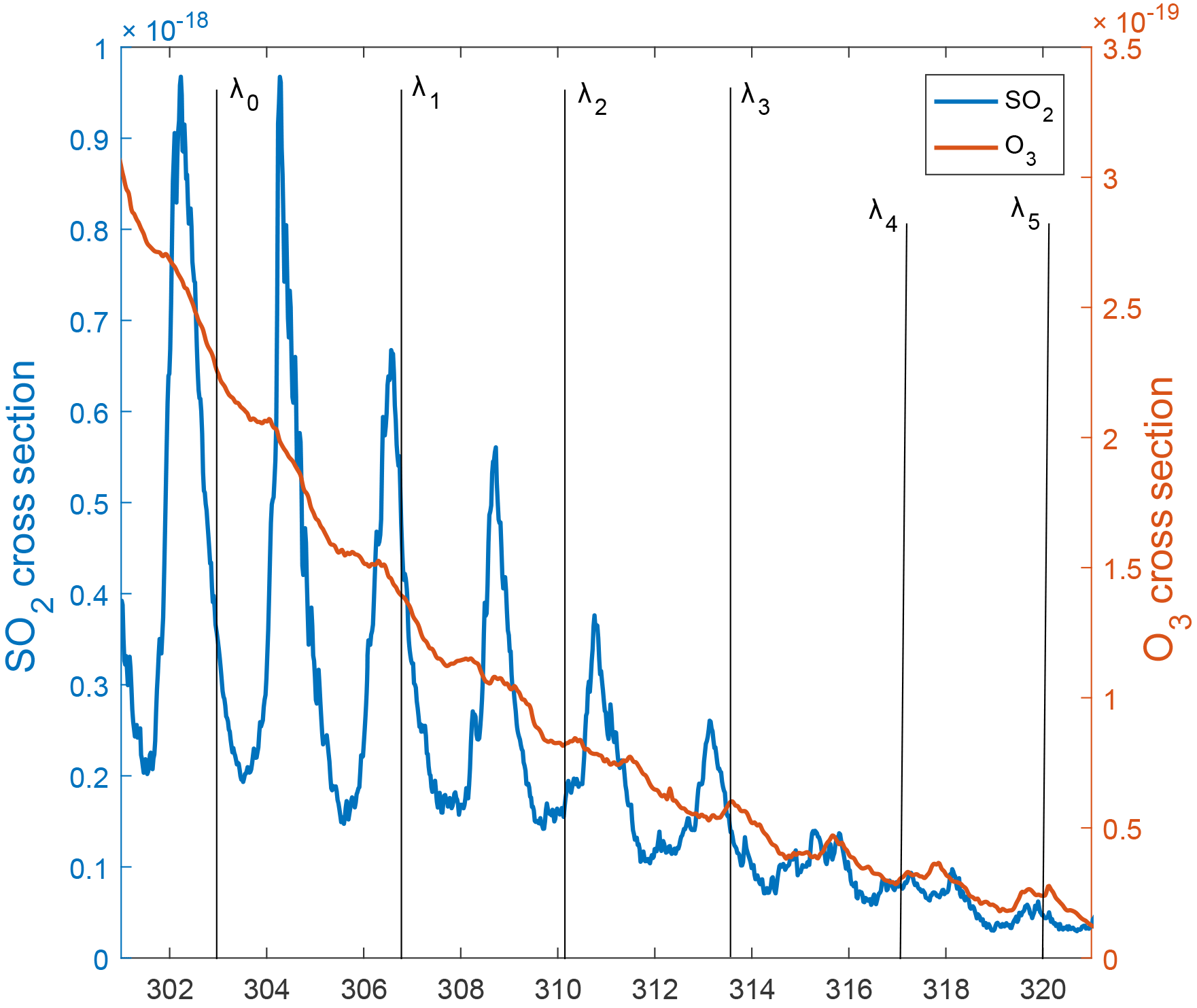
Figure 1 Ozone and sulfur dioxide absorption cross sections. The solar radiation is measured for the intensity bands (λ_1–5=306.4, 310.1, 313.5, 316.8, 320.0 nm). In contrast, the wavelength λ₀=303 nm is used for a checking routine.

The ozone absorption coefficient, α, is calculated from a dispersion test (Redondas et al., 2014a):

$$\begin{array}{}\text{(3)}& \mathit{\alpha }=\sum _i{w}_i{\mathit{\alpha }}_i,\end{array}$$

where α_i represents the band intensity calculated for each wavelength indicated in Fig. 1.

The weights, w_i = (−1, 0.5, 2.2, −1.7), and the wavelengths, λ_i = (310.1,313.5,316.8,320.0 nm), used have been especially selected to suppress the aerosol and SO₂ effects in the measured signal (Dobson, 1957; Kerr et al., 1981). These w_i and λ_i fulfil the Eqs. (4) and (5), ensuring that any linear effects with wavelength are suppressed and also allow any small shift in wavelength and the influence of SO₂ on the ozone retrieval to be minimized.

$$\begin{array}{}\text{(4)}& {\displaystyle }& {\displaystyle }\sum _{i=\mathrm{1}}{w}_i=\mathrm{0}\text{(5)}& {\displaystyle }& {\displaystyle }\sum _{i=\mathrm{1}}{w}_i{\mathit{\lambda }}_i\approx \mathrm{0}\end{array}$$

A more extensive description of the dispersion test and the mathematical procedure used to calculate the ozone concentration can be found in Gröbner et al. (1998) and Kipp & Zonen (2008). Finally, the ETC must be calculated directly using the Langley technique or calculated from the data comparison with a reference instrument.

2.2 Langley calibration method for the RBCC-E triad

The Langley technique is the most popular procedure that is able to estimate the extraterrestrial constant (ETC) used by the reference instruments. In practice, with respect to TOC measurements, the ETC can be calculated directly by fitting a linear equation to the MS9 values with respect to air mass μ:

$$\begin{array}{}\text{(6)}& \mathrm{MS}\mathrm{9}=\mathrm{ETC}+{\mathrm{O}}_{\mathrm{3}}\mathit{\alpha }\mathit{\mu },\end{array}$$

or using the Dobson method (Dobson and Normand, 1958; Komhyr et al., 1989):

$$\begin{array}{}\text{(7)}& {\displaystyle \frac{\mathrm{MS}\mathrm{9}-(\mathrm{ETC}+\mathrm{\Delta }\mathrm{ETC})}{\mathit{\mu }}}={\mathrm{O}}_{\mathrm{3}}\mathit{\alpha },\end{array}$$

where ΔETC represents the variation of this parameter with respect to a reference value.

Both equations can be used to calculate the ETC value to be used in Eq. (1) but Eq. (7), where the slope is inverse to μ, has the advantage of presenting a better data distribution (Kiedron and Michalsky, 2016). This is because the number of measurements taken at low air mass $(\mathrm{1}\le \mathit{\mu }\le \mathrm{2})$ is higher than that at large air mass (μ≥2). Although all measurements could be used for this calculation, experience suggests that is better to select a subset of measurements. The days with a high aerosol optical depth concentration, i.e. during Saharan dust intrusions, are removed from this study with the help of data reported by other instruments.

The methodology used is essentially the same as described in (Redondas, 2008; Redondas et al., 2014b). The following criteria, listed in order of application, can be used to get a good agreement between the ETC values calculated:

1. The regression is performed on the [1.25, 3.5] air mass range using the Brewer astronomical formulas for the air mass determination.

2. The data recorded during the morning and afternoon are taken separately (two Langley plots per day)

3. The TOC observation is calculated in the DS routine as the average of five single measurements, applying a cloud-screening filter (SD < 2.5 DU). However, in the Langley regression the individual measurements are used (and not the average) if these pass the cloud filter.

4. MS9 double ratios are corrected for filter non linearity.

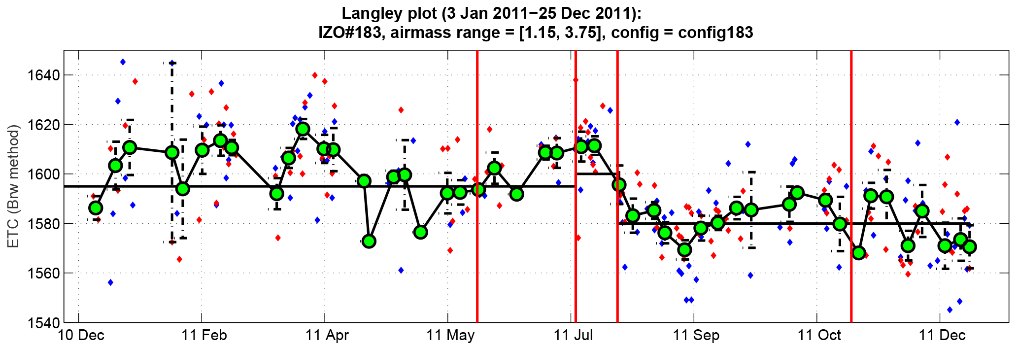
Figure 2 Operative ETC value for Brewer #183, after some events that could cause a change in the instrumental calibration during 2011. The red and blue dots denote daily ETC values calculated by the Langley method before and after solar noon, respectively. The circles and the error bars correspond to the ETC weekly mean and its standard deviation.

It is important to indicate that, despite selecting the better days on which the ETC values obtained for different days are compared, these present a standard deviation around ±5. This difference is considered normal and the ETC introduced in Eq. (1) corresponds to the ETC mean. Although the median can be another way of obtaining the ETC, the previous criteria guarantee that the difference between the methods is not significant.

Aside from determining the TOC, the ETC is used as a probe to check the correct state of the instrument. The ETC calculated from the Langley method presents a near constant value (SD ±5), changing only when the calibration of the instrument drifts. This may happen, for example, after replacing a damaged component or due to normal drifts by its continued operation. In both cases and after a stabilization period, a new ETC value can be calculated.

As an example, Fig. 2 shows the operative value of the ETC for Brewer #183 during the year 2011. The vertical lines represent situations which can produce a change in the behaviour of the instrument, while the horizontal line represents the operative ETC used to calculate the TOC (Eq. 1). As can be observed, the ETC changed twice, the first time by maintenance tasks (performed by IOS service in July 2011) and the second time due to changes in the Brewer configuration (to be more precise, changes in the wavelength calibration in August 2011). On the contrary, during the maintenance tasks (June 2011) or after UV calibration in our facilities (November 2011), the ETC remained constant. Only the Langley techniques that satisfy the conditions indicated in Sect. 2.2 are used to calculate the weekly mean. Other examples of events that may affect the ETC can be found in the calibration campaign reports (Redondas and Rodríguez-Franco, 2016; Redondas et al., 2015).

Routinely since 2009, monthly calibrations are run for the three instruments. This task is based on evaluating the following points:

1. The internal lamps that test historical records are analysed.

2. The Langley values and their comparison with the ETC operative are obtained in this period.

3. The values are reported by the checking routines of each instrument.

4. Our Brewer instruments are compared.

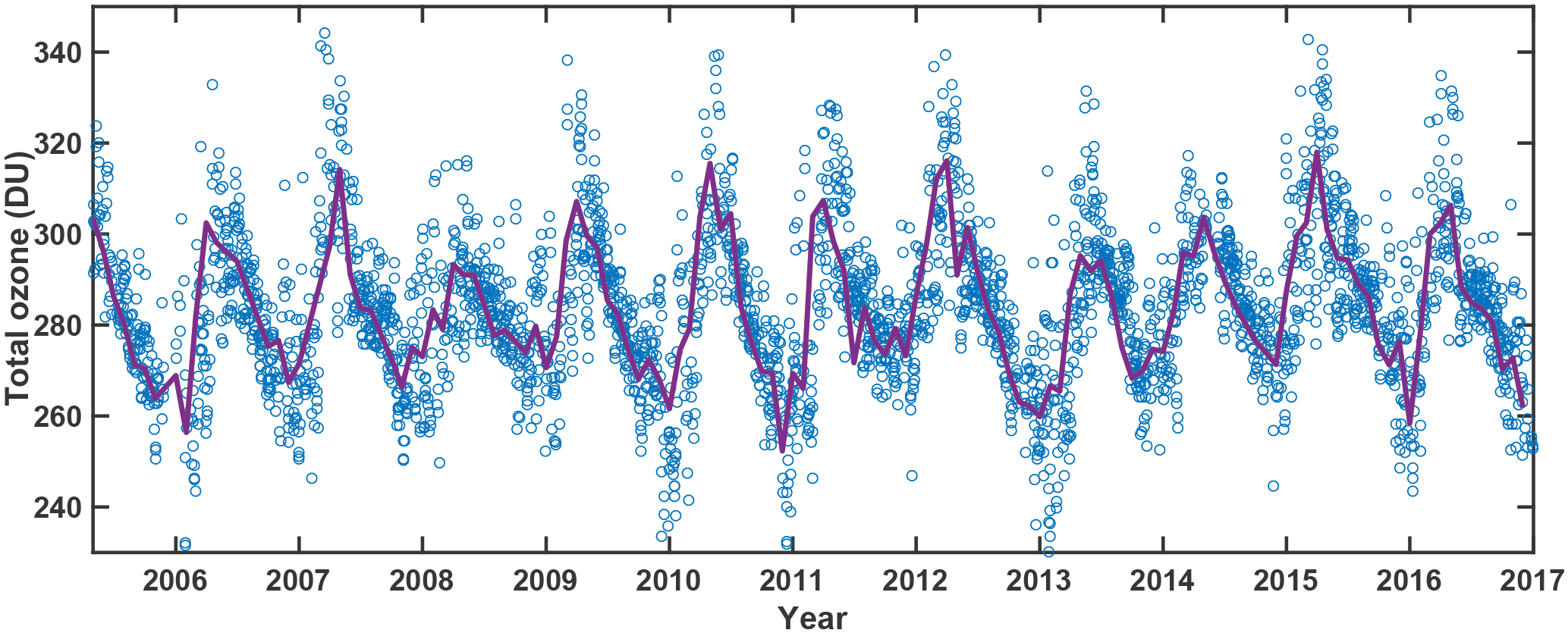
Figure 3 Time series of the ozone concentrations measured by Brewer #157 at Izaña Atmospheric Observatory, showing daily (dots) and monthly (line) means.

This procedure allows us to identify the exact moment at which a Brewer requires a new calibration. The calibration reports are available on the RBCC-E website; see for example (León-Luis et al., 2016). However, the ETC changes in Brewer instruments #157, #183 and #185 during the period 2005–2016 have been included in the Supplement. In addition, before and after the calibration campaign our travelling reference (Brewer#185) is compared with Brewer instruments #157 and #183, which remain at the observatory. The traceability between the RBCC-E and the world reference triads is checked in the calibration campaigns, organized by the RBCC-E, which compares observations of the travelling references, Brewer instruments #185 and #017. The results of these comparisons are shown in the calibration campaign reports (Redondas and Rodríguez-Franco, 2015, 2016; Redondas et al., 2015) and summarized in Table 2 of Redondas et al. (2018).

3 Ozone and selected data set

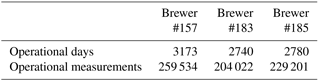
In order to summarize the history of the RBCC-E Brewer instruments, Table 1 provides the total number of days and measurements taken by these instruments since they became operational at IZO and as long as the weather conditions allowed them to operate. Figure 3 shows the daily and monthly TOC means measured by Brewer #157. The ozone presents an annual cycle with a sawtooth profile with maximum and minimum values in spring and autumn, respectively. Despite this annual behaviour, the ozone presents a lower daily variability as indicated by our measurements. This factor, together with a thermal inversion, which produces an atmosphere free of anthropogenic pollutants and excellent weather conditions all year, except for days with Saharan dust intrusions, explain why Izaña Atmospheric Observatory is an excellent location for a Brewer reference centre and also why the Langley technique is used as calibration method.

Table 1 Number of operational days and measurements since their set-up for the Brewer instruments of the RBCC-E triad.

In this work, the ozone data sets have been analysed. The first data set is obtained directly after applying several conditions listed here in order of application:

1. Only include measurements taken at Izaña Atmospheric Observatory.

2. Remove days with problems clearly identified (wrong alignment, etc.).

3. Only the days where the three Brewer instruments have taken measurements are considered in this work. Moreover, each Brewer must have more than 12 measurements, with a minimum of 4 before and after the solar noon (homogeneous distribution).

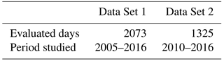
The second data set is obtained with the same conditions but also imposing the condition that the measurements must be simultaneous in time. A measurement is considered simultaneous if we have one observations of each instrument in a temporal window of 5 min. Therefore, this second data set can be considered a subset of the first. Table 2 gives a summary of both data sets. The entry “evaluated days” denotes the number of days used in each data set to study the consistency of the RBCC-E triad. It is important to note that Data Set 1 includes the measurements made in the period 2005–2016, while Data Set 2 only considers simultaneous measurements from 2010 onwards. Before 2010, a large part of the measurement time was focused on the UV spectrum, and hence there are fewer ozone direct sun measurements in the instrument schedule. This means that the likelihood of finding 12 simultaneous measurements between the three instruments is low, particularly in winter when the presence of clouds is greater. After 2010, The RBCC-E started using the same synchronization schedule in their Brewer instruments. These schedules take into account the sunrise and sunset times of each day and the introduced routines are distributed as a function of the solar zenith angle (SZA).

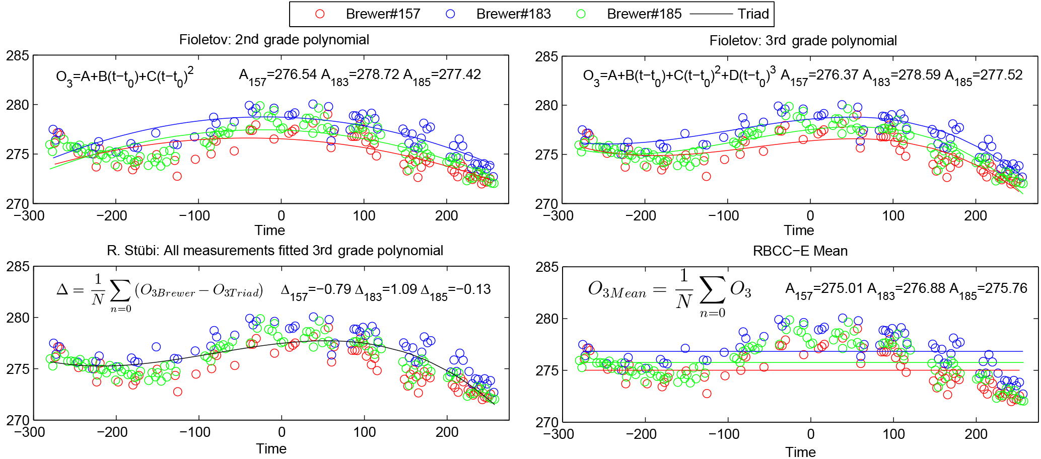
Figure 4 Method used to calculated the daily representative value. The ozone values plotted were measured on 16 November 2016.

4 Results and discussion

The consistency of the measurements carried out by the RBCC-E triad was evaluated from the data sets described in Sect. 3. In the case of the long-term behaviour, it was studied using both data sets, while the short-term behaviour was analysed using only Data Set 1. The results obtained are shown in statistical terms.

4.1 Representative value of the total ozone column

To our knowledge, there are only a few publications in which the consistency of the world reference and Arosa triads are analysed. In these articles, and due to the large number of ozone measurements taken each day, the authors have calculated a representative value of all of them and, from it, the long-term consistency is analysed (Fioletov et al., 2005; Scarnato et al., 2010; Stübi et al., 2017).

Fioletov et al. (2005) studied the long-term consistency of the world reference triad in the period 1985–2003. In this work, the authors proposed to fit the measurements taken by each Brewer (#008, #014 and #015) to a second-grade polynomial (see Fig. 4):

$$\begin{array}{}\text{(8)}& {\mathrm{O}}_{\mathrm{3}}=A+B\cdot (t-t_{\mathrm{0}})+C\cdot (t-t_{\mathrm{0}}{)}^{\mathrm{2}},\end{array}$$

where O₃ is the TOC measured and t−t₀ corresponds to the difference between the time of the measurement and the solar noon. The independent coefficient A obtained through the adjustment is used as a representative ozone value of each instrument. The difference between this coefficient for each Brewer and the triad mean represents the daily drifts of each instrument. The consistency is studied from the relative standard deviation of these differences. In this work, the results using a third-grade polynomial have also been investigated; see Fig. 4.

Table 2 Summary of the data sets used in this work.

Stübi et al. (2017) studied the long-term consistency of the Arosa triad in the period 1988–2015. In this study, the authors considered that the behaviour of the triad is the most appropriate reference for each day. Therefore, all the measurements made by the three Brewer instruments are modelled as a third-grade polynomial dependent on time, which represents the triad (see Fig. 4):

$$\begin{array}{}\text{(9)}& {\mathrm{O}}_{\mathrm{3}}=A+B\cdot (t-t_{\mathrm{0}})+C\cdot (t-t_{\mathrm{0}}{)}^{\mathrm{2}}+D\cdot (t-t_{\mathrm{0}}{)}^{\mathrm{3}}\end{array}$$

where t₀ corresponds to 12:00 UTC. In this case, each Brewer can be characterized by a shift, Δ, which is the daily mean of the difference between the values measured and obtained from the fit and a standard deviation, σ, which evaluates the dispersion of these differences. Both parameters are used to analyse the long-term consistency of the Arosa triad.

In order to compare the long-term consistency of the RBCC-E triad with respect to the world reference and Arosa triads, both methods are used to fit our measurements. However, in this work, the time reference t₀ is the solar noon.

Although Eqs. (8) and (9) are valid to model the behaviour of ozone, it should be noted that the normal drifts by its continued operation of the instrument can affect the final value of the adjustment. Given this problem, calculating the daily mean of the measurements can be a good strategy to avoid this inconvenience. In this work and our measurements ozone presents a reduced daily variability (see Fig. 4) and the mean of the all measurements, N, made by each Brewer was used as a representative value.

$$\begin{array}{}\text{(10)}& A_M={\displaystyle \frac{\sum _i{\mathrm{O}}_{\mathrm{3}}}{N}}\end{array}$$

The difference between the value obtained for each Brewer and the triad mean represents the drifts of each instrument. Although the median can be used to study the behaviour of the RBCC-E triad, our experience suggests that the daily mean is robust. Moreover, since 2003, the mean has been used to detect when one of our Brewer instruments loses its calibration; therefore it is worth including it in this work. At this point, it is important to note that, for the world reference triad as for the RBCC-E, the representative value of each instrument is calculated directly from their measurements. In contrast, in the Arosa triad, the representative value of each instrument (denoted as shift Δ) is calculated with respect to the behaviour of the three instruments, obtained by adjusting the observations to a polynomial of the third degree (see Fig. 4).

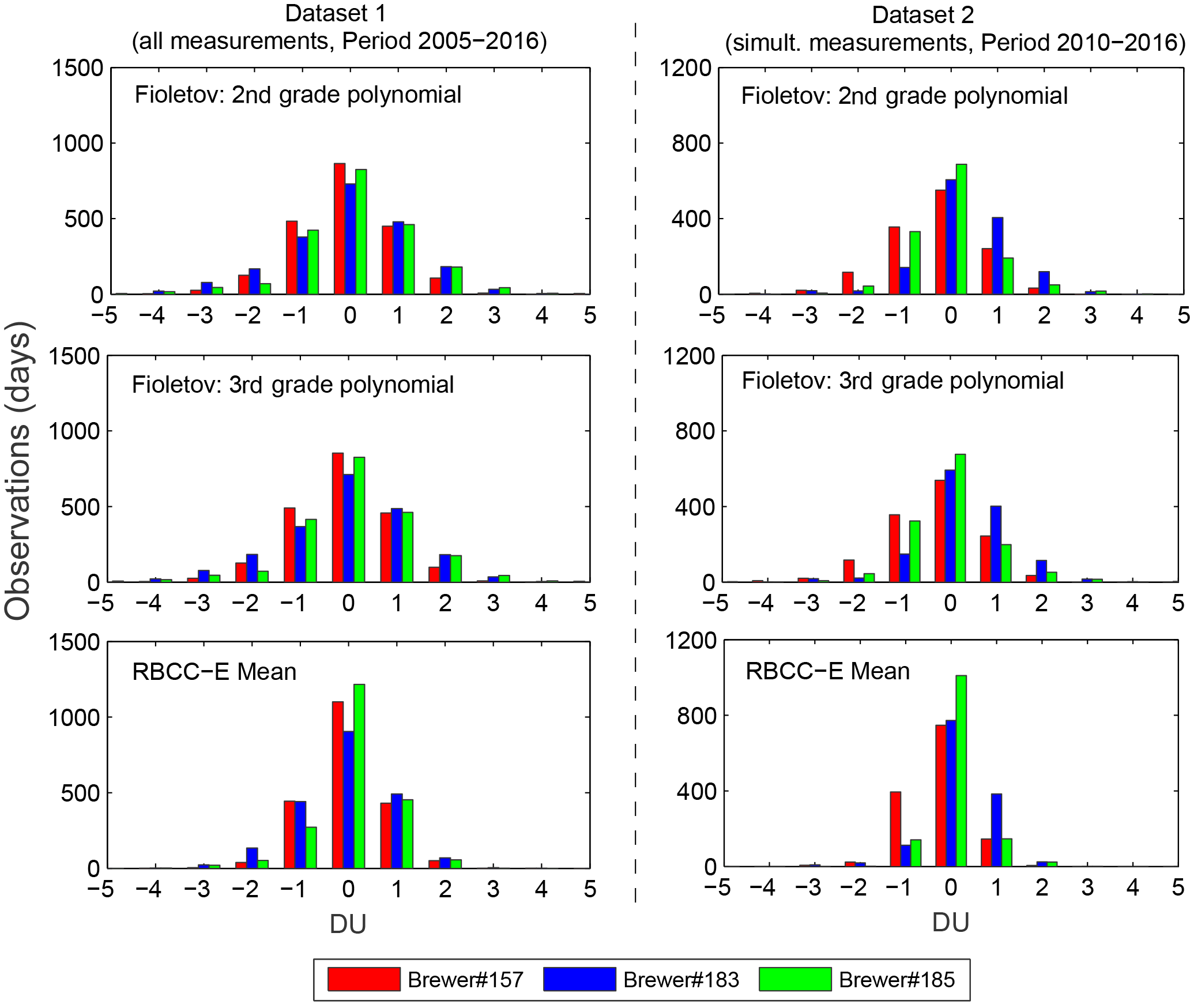
Figure 5 Daily difference of the ozone reference value A of each Brewer with respect to the triad. The values were obtained from the procedure proposed by Fioletov (world reference triad) and by daily mean (RBCC-E).

4.1.1 Long-term consistency: daily averages

Following the procedure described by Fioletov et al. (2005) for the world reference triad, data sets 1 and 2 (see Sect. 3) were fitted by a second- and third-grade polynomial as is shown in Fig. 4. The distribution of the daily difference between the A values (see Eq. 8), obtained for each Brewer with respect to the triad mean are plotted in Fig. 5. Also, in this plot, the difference calculated from the daily mean of each instrument was included; see Eq. (10). It is important to take into account the individual coefficients obtained for each Brewer and also the triad mean calculated from them, depending on the method used.

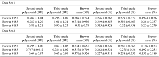
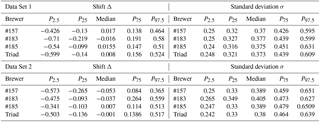
Table 3 Absolute and relative values of the mean shift and the standard deviation.

As Fig. 5 shows, the histograms that represent the results obtained when a polynomial fit is used in each data set are independent of its grade. This can be explained by the small daily variation of the ozone which causes the second- and third-grade polynomial fit to give very similar A coefficients; see Fig. 4. In contrast, the histograms associated with the daily mean suggest that the differences between the Brewer instruments are less. This allows us to conclude that the method selected to evaluate the consistency plays an important role, because the Brewer-triad mean differences are directly associated with it. In this case, it may be more appropriate to use the daily mean to evaluate the RBCC-E triad. Independently of the method used, Fig. 5 shows that, for the great majority of days, the Brewer instruments present less than 2 DU of the difference with respect to the triad mean, which indicates a good agreement among themselves.

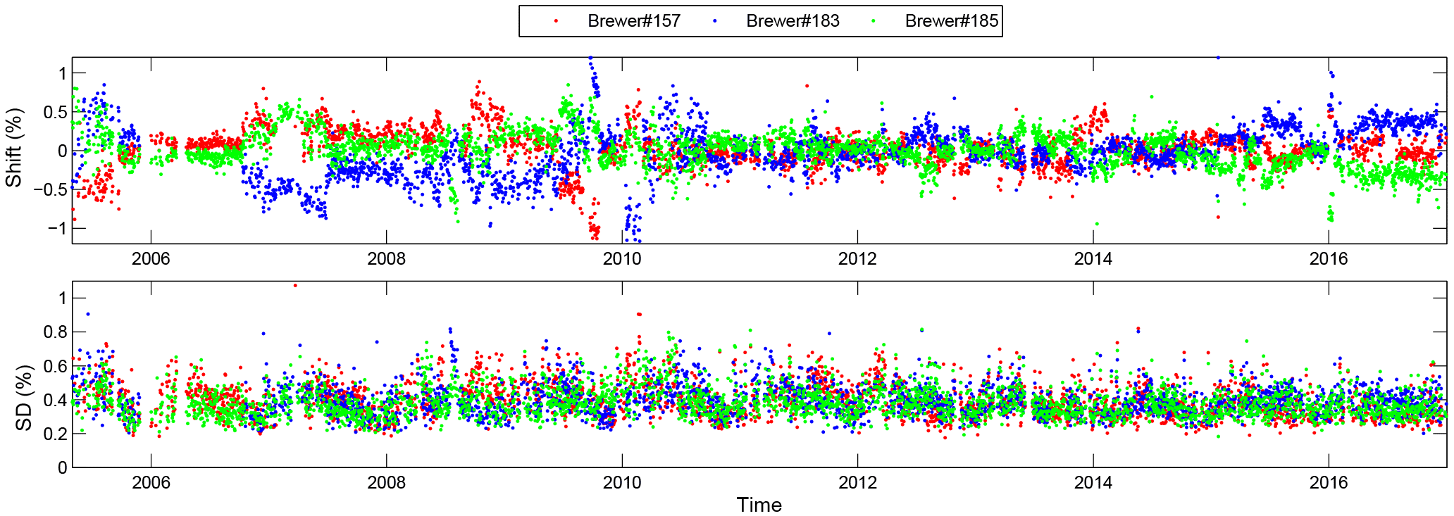
Figure 6 Time series of the mean shift Δ and the standard deviation σ, relative to the TOC calculated from measurements by the three Brewer instruments of the RBCC-E triad (#157, #183 and #185) fitted with a third-grade polynomial.

Using the same procedure to evaluate the long-term consistency can be the best strategy for comparing different triads to each other. In this sense, Fioletov et al. (2005) only reported that the relative daily standard deviation of the world reference triad is equal to 0.47 %. This value was calculated as the mean of the relative standard deviation of each Brewer. Table 3 contains the mean difference, calculated from the mean Brewer triad difference plotted in Fig. 5, and its standard deviation. The RBCC-E triad presents a relative standard deviation mean equal to 0.41 % (σ₁₅₇=0.362 %, σ₁₈₃=0.453 % and σ₁₈₅=0.428 %; see Table 3, Data Set 1, 4th column). This result indicates that the dispersion of the measurements of the RBCC-E Brewer instruments presents a similar behaviour to those of the world reference triad. Furthermore, the obtained standard deviation values confirm that the daily mean is the best method with which to evaluate the RBCC-E triad.

In order to compare the daily behaviour of the Arosa and RBCC-E triads, a third-grade polynomial was fitted to all the daily measurements made by RBCC-E Brewer instruments for data sets 1 and 2. Then, for each Brewer its mean shift, Δ, and standard deviation, σ, were calculated (see Sect. 3). The values obtained for Data Set 1 are shown in Fig. 6. Because Brewer #183 was damaged by a storm and was inoperative between December 2005 and September 2006, the data plotted in that period were calculated from measurements of Brewer instruments #157 and #185 only. Similarly, when Brewer #185 is away from IZO in calibration campaigns, the values plotted correspond to Brewer instruments #157 and #183. Note that, although these data were introduced in Fig. 6 to avoid gaps in the plot, they are not considered in the statistical study. Therefore, the evaluated dates correspond with the days when the full RBCC-E triad is operative, and the criteria established in Sect. 3 are still used.

Table 4 Percentiles of the difference distribution (%) for the RBCC-E triad.

As can be observed in Fig. 6, the results obtained for all instruments in Data Set 1 show a (±0.5) value for the mean shift. A similar result was obtained for Data Set 2 (figure not shown). Similarly reported by Stübi et al. (2017), the standard deviation shows a small seasonal component. This result is explained by the low daily variability of the ozone at subtropical latitudes. For the Brewer instruments of the RBCC-E triad, the standard deviation is more influenced by anomalous internal behaviour of the instruments. For midlatitudes, e.g. in Arosa, there is a larger daily variation in ozone, shown by the standard deviation.

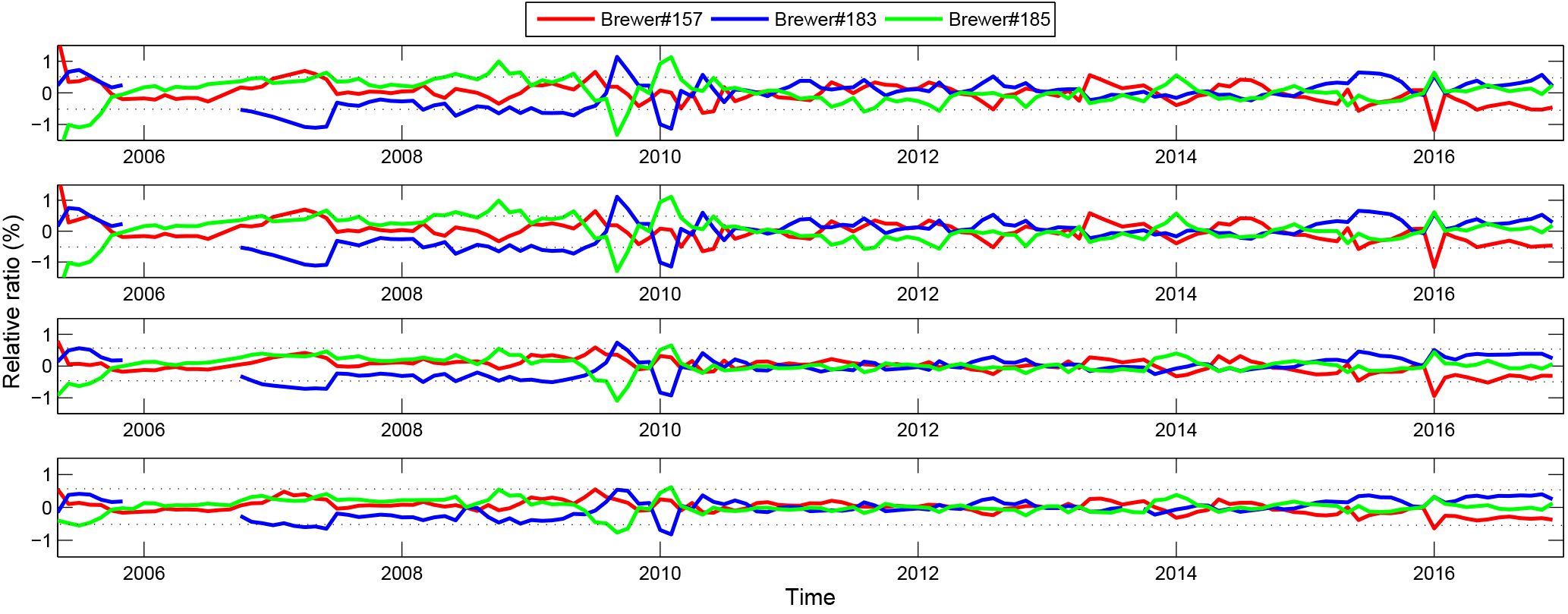
Figure 7 Relative ratio of the monthly values with respect to the triad mean for the methods proposed for the world reference triad (Fioletov et al., 2005), daily mean (RBCC-E) and Arosa triad (Stübi et al., 2017). The gap for the Brewer #183 data was caused by the tropical storm Delta, which damaged the instrument. In 2010, Brewer #183 had a problem with a stepper motor micrometer.

Following Stübi et al. (2017), Table 4 shows the distribution of percentiles of the mean shift and the standard deviation values plotted in Fig. 6. The Brewer instruments present a similar interpercentile range P_2.5–P_97.5, with a mean value close to 1.1 %. This result is consistent with the standard deviation shown in Table 3 for the polynomial fits. In comparison with the Arosa triad, only Brewer #040 shows better behaviour than the RBCC-E Brewer instruments, while other Brewer instruments (B#072, B#156) show values similar to ours.

4.1.2 Long-term consistency: monthly averages

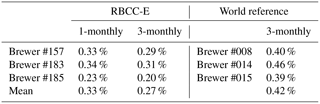
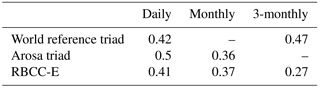
The histogram and the statistical parameters already presented suggest that the long-term consistency of the RBCC-E, Arosa and world reference triads are similar, but it can be more interesting to present this study from the monthly means. With this idea in mind, the daily difference plotted in Fig. 5 and the daily shift plotted in Fig. 6 were averaged over months. Figure 7 shows, in relative terms, the monthly values for the period 2005–2016 (Data Set 1). The results confirm that the RBCC-E triad has good long-term precision, regardless of the method selected. In order to compare it with the world reference triad, Table 5 contains the relative standard deviation of the difference between the representative value A of each Brewer, calculated from the second-grade polynomial fit, and the triad mean. As reported by Fioletov et al. (2005), the relative standard deviations of the 3-monthly mean for the world reference triad are 0.40, 0.46 and 0.39 % for Brewer instruments #008, #014 and #015, respectively (0.42 % in mean). The RBCC-E Brewer instruments have lower 1-monthly and 3-monthly relative standard deviation. The ratio between 3-monthly standard deviation is 36 % lower for the RBCC-E.

Furthermore, Stübi et al. (2017) reported that in the period 2004–2012 the Arosa triad presented a monthly shift around ±0.4 %, while the RBCC-E are lower than ±0.3 %.

Table 5 RBCC-E and world reference triads: relative monthly standard deviations.

4.2 Short-term consistency

Data Set 2 was used to study the short-term consistency of the RBCC-E triad, with the aim to determine in which SZA range the consistency of the measurements is higher. The measurements taken by the three Brewer instruments every day were fitted using a third-grade polynomial as shown in Fig. 8. As previously commented, this polynomial represents the behaviour of the triad and allows the TOC to be obtained as a function of time. Similarly to the previous study, each Brewer was characterized by a shift Δ. In this case, the data were divided as a function of the SZA. Different SZA ranges were checked and it was found that the analysis can be reduced to just three broad ranges:

1. SZA > 60^∘ corresponds to the first and last ozone measurements of every day, when solar radiation presents a low intensity and high Rayleigh scattering.

2. SZA < 30^∘ corresponds to the measurement in the middle of the day, when the air mass is close to 1 and hence there is less Rayleigh scattering.

3. 60^∘ < SZA < 30^∘ comprises the rest of ozone measurements.

Figure 8 (a) Experimental measurements and third-grade triad fit and (b) relative difference by Brewer as function of the SZA. The drop is due to one Brewer was not operating for a few minutes and hence there are no simultaneous measurements between the three instruments.

In Fig. 8, the box plot shows the statistical distribution of the mean shift calculated for the selected ranges. As can be observed, the greatest dispersion values are at low SZA, which indicates solar noon, when more discrepancy can be observed between the data recorded by the instruments. This result may seem surprising because in these conditions the solar radiation on the Earth's surface is maximum and the Rayleigh scattering is minimum but it can be easily explained from Eq. (1). In this expression, at low SZA the optical mass, μ, is close to 1 and the ozone absorption α is a constant value. This implies that the denominator takes an almost constant value. Therefore, a small fluctuation (noise) associated with the MS9 values may significantly affect the recorded TOCs. In contrast, for the other ranges the denominator takes a significant value and the effect of the noise on MS9 is smaller, increasing the consistency of the measurements. In addition, the Fig. 8 shows that Brewer #183 presents poorer results, which can be explained if it is taken into account that this instrument was damaged in 2007, and during 2008 it had an irregular operation. Moreover, in 2010, it had a problem with a stepper motor micrometer (Roozendael et al., 2013).

5 Conclusions

The long-term consistency of the TOC measurements made by the RBCC-E triad has been studied and compared with the values reported for the world reference and Arosa triads. With this idea in mind, the procedure described by Fioletov et al. to evaluate the TOC measurements made by the world reference triad was used in this work. The relative daily standard deviation for each Brewer, σ₁₅₇=0.362 %, σ₁₈₃=0.453 %, and the triad mean, σ=0.41 %, were calculated. The values obtained for RBCC-E are lower than the reported value for the world reference triad. Also, in this work the possibility of extending the fitting proposed by Fioletov et al. (2005) to a third-grade polynomial has been investigated. In this case, for our TOC measurements, there is no significant improvement of the results compared to the initially proposed fitting. As the world reference, the RBCC-E calculated the relative 1-monthly and 3-monthly standard deviation as the average of the daily values.

Table 6 Summary of the three studies comparing the relative standard deviations of the world reference triad, Arosa and RBCC-E triads.

The standard deviations calculated from the procedures by Fioletov et al. (2005) and Stübi et al. (2017) are not equal but they are similar enough to compare the three triads. In this table, the values introduced for the RBCC-E were obtained from the procedure used by Fioletov et al. (2005) for the world reference triad.

In addition, applying the procedure described by Stübi et al. (2017) to study the Arosa triad, the RBCC-E triad presents a similar interpercentile range P_2.5–P_97.5, with a value close to 1.1 %, similar to those reported for the Arosa triad, except in the case of Brewer #040. Although the methodology used to study the world reference and Arosa triads are different, the standard deviation reported for these and RBCC-E triads are fairly similar, which indicate a large level of internal consistency between their instruments (see Table 6). However, sin order to guarantee correct traceability of the ozone measurements all around the world, a greater frequency of Absolute Calibration Campaign between the calibration centre and the travelling standard reference is necessary.

Finally, the short-term consistency between the TOC measurements made by our Brewer instruments is investigated. For this, the TOC observations were divided as a function of the SZA. The results indicate that a greater difference between the observations is seen at midday.