the Creative Commons Attribution 4.0 License.
the Creative Commons Attribution 4.0 License.
 | 17 Jul 2018
Correction of CCI cloud data over the Swiss Alps using ground-based radiation measurements
Fanny Jeanneret
Giovanni Martucci
Simon Pinnock
Alexis Berne
The validation of long-term cloud data sets retrieved from satellites is challenging due to their worldwide coverage going back as far as the 1980s. A trustworthy reference cannot be found easily at every location and every time. Mountainous regions present a particular problem since ground-based measurements are sparse. Moreover, as retrievals from passive satellite radiometers are difficult in winter due to the presence of snow on the ground, it is particularly important to develop new ways to evaluate and to correct satellite data sets over elevated areas.
In winter for ground levels above 1000 m (a.s.l.) in Switzerland, the cloud occurrence of the newly released cloud property data sets of the ESA Climate Change Initiative Cloud_cci Project (Advanced Very High Resolution Radiometer afternoon series (AVHRR-PM) and Moderate-Resolution Imaging Spectroradiometer (MODIS) Aqua series) is 132 to 217 % that of surface synoptic (SYNOP) observations, corresponding to a rate of false cloud detections between 24 and 54 %. Furthermore, the overestimations increase with the altitude of the sites and are associated with particular retrieved cloud properties.
In this study, a novel post-processing approach is proposed to reduce the amount of false cloud detections in the satellite data sets. A combination of ground-based downwelling longwave and shortwave radiation and temperature measurements is used to provide independent validation of the cloud cover over 41 locations in Switzerland. An agreement of 85 % is obtained when the cloud cover is compared to surface synoptic observations (90 % within ± 1 okta difference). The validation data are then co-located with the satellite observations, and a decision tree model is trained to automatically detect the overestimations in the satellite cloud masks. Cross-validated results show that 62±13 % of these overestimations can be identified by the model, reducing the systematic error in the satellite data sets from 14.4±15.5 % to 4.3±2.8 %. The amount of errors is lower, and, importantly, their distribution is more homogeneous as well. These corrections happen at the cost of a global increase of 7±2 % of missed clouds. Using this model, it is possible to significantly improve the cloud detection reliability in elevated areas in the Cloud_cci AVHRR-PM and MODIS-Aqua products.
- Article
(13685 KB) - Full-text XML
- BibTeX
- EndNote


Clouds have a major importance in climate: they play a key role in the radiation budget (Trenberth, 2009) and the water cycle, which then impact almost every component of the climatic system. As the climate changes, cloud properties change as well (Davies et al., 2017; Norris et al., 2016; Quaas, 2015). Detecting and analysing these changes is only possible with high-quality data sets spanning several decades. Satellite instruments are the most suitable tools for the global observation of clouds, and scientific effort is increasingly focusing on reprocessing historical records to extract as much information as possible from them. In 2010, the European Space Agency started the Climate Change Initiative (CCI) programme (Hollmann et al., 2013) to coordinate scientific work towards the production, homogenisation, and validation of long-term data sets constructed from different satellite instruments. The CCI project dedicated to clouds, the Cloud_cci Project (Stengel et al., 2015), is releasing its open data sets at the time of writing of this paper. Two of them are of particular interest here: the data set based on the Advanced Very High Resolution Radiometer afternoon series (AVHRR-PM) and the data set based on Moderate-Resolution Imaging Spectroradiometer (MODIS) Aqua data. AVHRR-PM has a long time coverage, which gives the opportunity to look for climate change signals. The MODIS-Aqua data set is processed by the Cloud_cci using the same algorithm (McGarragh et al., 2018; Sus et al., 2018) as AVHRR-PM, only with a higher spatial resolution.
In mountainous regions, processes such as elevation-dependent warming (Pepin et al., 2015; Rangwala and Miller, 2012) are documented, suggesting climate might change faster with increasing altitude. Thus, signs of climate change should be easier to observe in elevated areas, due either to larger amplitudes or to earlier appearance. However, mountains are one of the most challenging places for satellite measurements: the accuracy of geolocation is lower over complex terrain, and radiometers measurements often lack sufficient information to clearly discriminate between snow and clouds (Musial et al., 2014). As a consequence, data sets based only on satellite radiometers have a lower quality in winter in mountainous areas, and this study proposes a way of addressing this limitation by combining ground-based information and machine learning techniques.
Ground-based data have long been used to estimate cloud cover, for instance synoptic observations (Barbaro et al., 1981); passive measurements of shortwave (Long et al., 2006; Martínez-Chico et al., 2011; Pagès et al., 2003), longwave (Dürr and Philipona, 2004; Herrmann et al., 2015), and microwave radiation; and active instruments such as cloud radars and lidars. The latter ones can indisputably provide accurate measurements of cloud properties like occurrence, altitude, and lifetime, but due to their cost they are quite rare and often do not have long historical records. This study hence combines measurements of downwelling longwave and shortwave radiation to detect cloud occurrence at 41 locations in Switzerland. This new ground-based cloud information (henceforth referred to as a “cloud mask”) covers the period from 1995 to the end of 2014, with different lengths (6.1 ± 4.8 years on average) at different locations, and is validated against synoptic observations for 24 of the 41 stations.
Once the ground-based cloud mask is computed from the radiation data, it is used as a reference to train an automated algorithm to detect false cloud measurements in the satellite pixels at the 41 locations. A brief analysis of the types of situations inducing the retrieval algorithm errors is conducted. Time series of cloud properties are also presented, as well as the impact of the removal of points identified as false clouds by the model trained in this study. Then, after investigating the possibilities for spatial extrapolation, the algorithm is applied to every satellite pixel in a defined area to identify false clouds when and where no information about the true cloud cover is available. As the focus of this study is on mountainous areas, the geographical zone of interest covers the Swiss Alps. The time frame is 1982–2012 for the AVHRR-PM data set and 2002–2014 for MODIS-Aqua.
In this section, an overview of the problems encountered when using two data sets of the Cloud_cci in mountainous regions is presented. The characteristics and limitations of the two data sets are summarised, and cloud occurrences in the European Alps are shown as an example. A local validation test is made using 24 ground-based stations in Switzerland and shows that, when snow is present in the retrieval pixel, cloud amounts are significantly overestimated.
2.1 CCI data sets
Two open data sets of the Cloud_cci are used: the first one is derived from the AVHRR instruments (Cracknell, 1997) on board seven satellites of the US National Oceanic and Atmospheric Administration (NOAA). The second data set is from the MODIS instrument (Barnes et al., 1998) on board Aqua, one of the A-Train satellites of the US National Aeronautics and Space Administration (NASA). These instruments are passive spectroradiometers measuring top-of-atmosphere radiances at five channels, the so-called AVHRR-heritage channels, centred approximately at 0.6, 0.8, 3.7, 11, and 12 µm. AVHRR on NOAA-16 had a different setup: a 1.6 µm channel was used in daytime instead of the 3.7 µm channel, until this was changed to the same setup as the others in May 2003. For consistency with AVHRR-based data sets, the Cloud_cci MODIS data sets are based on MODIS-Aqua measurements made at these five wavelengths even though the instrument measures at 36 different channels in total.
The Level 3U (corresponding to Level 2 uncollated data mapped onto a spatial grid), version 2 of the data sets was used (DOIs can be found in the references, under Stengel et al., 2017b, c). The AVHRR-PM data set covers the years 1982–2012 and has a resolution of 0.05∘ lat–long; MODIS-Aqua spans from 2002 to 2012 and is mapped onto a 0.02∘ lat–long grid over Europe. All instruments are on polar-orbiting, Sun-synchronous satellites and overpass locally in early afternoon (around 13:00) and early morning (around 01:00). Since the orbits of the NOAA satellites were allowed to drift, the local time of each AVHRR observation also drifts by several hours over the lifetime of each satellite (Heidinger et al., 2014).
Cloud properties are retrieved from the satellite-measured radiances using an optimal estimation approach, following the theoretical basis for inverse retrieval methods described in Rodgers (2004). The algorithm, called CC4CL, works in three steps: first, a neural network trained on co-located data from CALIOP (Cloud–Aerosol Lidar with Orthogonal Polarization) on board CALIPSO (Cloud–Aerosol Lidar and Infrared Pathfinder Satellite Observations) (Winker et al., 2009) is run on the measured radiances to determine if a cloud is present or not. Then, the cloud phase is determined with a decision tree, as proposed by Pavolonis and Heidinger (2004) and Pavolonis et al. (2005). Lastly, the retrieval is done using the measured radiances and some ancillary data such as atmospheric pressure, temperature and ozone, snow and ice cover, and land and sea surface temperature, all coming from ECMWF ERA-Interim (Dee et al., 2011), along with surface reflectance from the MODIS MCD43C1 product (Schaaf et al., 2010). The cloud top pressure (CTP), cloud optical thickness (COT), and cloud effective radius (CER) are returned directly by the optimal estimation, whereas the cloud top height, cloud top temperature, cloud albedo, and liquid and ice water path are then inferred from them. For more information, the algorithm is described in detail in Sus et al. (2018) and McGarragh et al. (2018).
As detailed in Stengel et al. (2017a), one of the particularities of these data sets is that they include uncertainty estimates at all processing levels. Validation of the Cloud_cci data sets is described in Stapelberg et al. (2017), but as it was done for the whole Earth, topographic details are not necessarily taken into account. In that report, false-alarm rates above 25 % are often seen to occur during daytime above polar snow- and ice-covered surfaces, which might be observed above high-elevated areas as well. When compared to CALIPSO-CALIOP (a satellite lidar instrument), more than 50 % of clouds under 0.15 optical thickness in the CALIOP data set is missing in AVHRR-PM and MODIS-Aqua data sets. Comparison of cloud occurrences with SYNOP observations (described in the next section) shows a good agreement of the seasonal cycles but overestimations (5 to 10 %) during winter in the Northern Hemisphere, particularly mid-latitudes in Europe and Asia.
2.2 Visual observations
Surface synoptic (SYNOP) observations are done every 3, 6 or 12 h at manned meteorological stations: an observer looks at the sky, mentally separating it into an eight-slice pie of which they would be the centre. For each of the eight sky slices, the observer determines if clouds are present and, if so, estimates their type and altitude. The cloud coverage is hence evaluated in numbers from 0 to 8 called oktas, with an extra value 9 for totally obscured sky (by fog or other meteorological phenomena; these values were discarded). Twenty-four stations in Switzerland are used in this study (a detailed list with operational times can be found in Table A1 in the Appendix). The exact observation time is not available, but it spans between 11:45 and 12:00 UTC.
To ease the comparison with the satellite's binary cloud masks, a limit was set at 0–3 oktas for clear skies and 4–8 oktas for cloudy skies, which means that only significant amounts of reported clouds will be categorised as cloudy conditions. It is consistent with the different viewing geometries involved, since the human observer might see much further than the satellite pixel's limits when the cloud cover is relatively sparse. Other thresholds were tested and confirmed that a 3-okta threshold is an optimal compromise between classifying too many and not enough situations as cloudy. This value is further confirmed by Bojanowski et al. (2014), who use the same threshold.
As the satellites overpass in early afternoon, their observations can be matched to SYNOP observations done at 12:00 UTC at the 24 stations in Switzerland. At every location, the SYNOP observations are compared with the satellite data falling in the corresponding pixel (approximately 1 × 1 km2 for MODIS-Aqua and 4 × 4 km2 for AVHRR-PM) between 11:40 and 12:20 UTC. The uncertainty of the comparisons are unknown, since SYNOP observations are not provided with uncertainties. The satellite cloud masks do not have associated data quality flags either. For SYNOP observations, known sources of uncertainties are the subjectivity of human observations and their inevitable variation from one observer to another (Mittermaier, 2012); the scenery effect (Karlsson, 2003; Malberg, 1973; Werkmeister et al., 2015) which increases the difficulty of comparing two different observation geometries, as cloud fractional cover tends to be overestimated by a ground-based observer looking in a slanted way at clouds spread vertically, especially when clouds are low on the horizon; and the detection difference between a human eye limited to the visible spectra and satellite sensors, which have wider spectral ranges, especially infrared wavelengths.
2.3 Satellite cloud mask
A geographical area centred in the Alps was defined as the area of interest for this study: it spans from 40 to 51∘ N and from 3 to 20∘ E (Fig. 1). In this area, the MODIS data set's cloud mask was averaged by season, and winter and summer averages are presented in Fig. 2. As can be observed, mountain reliefs are systematically associated with an increase in cloud occurrence, especially in winter. The same pattern is observed when averaging the cloud mask of the AVHRR-PM data set but cannot be found in ERA-Interim cloud mask data (not shown).
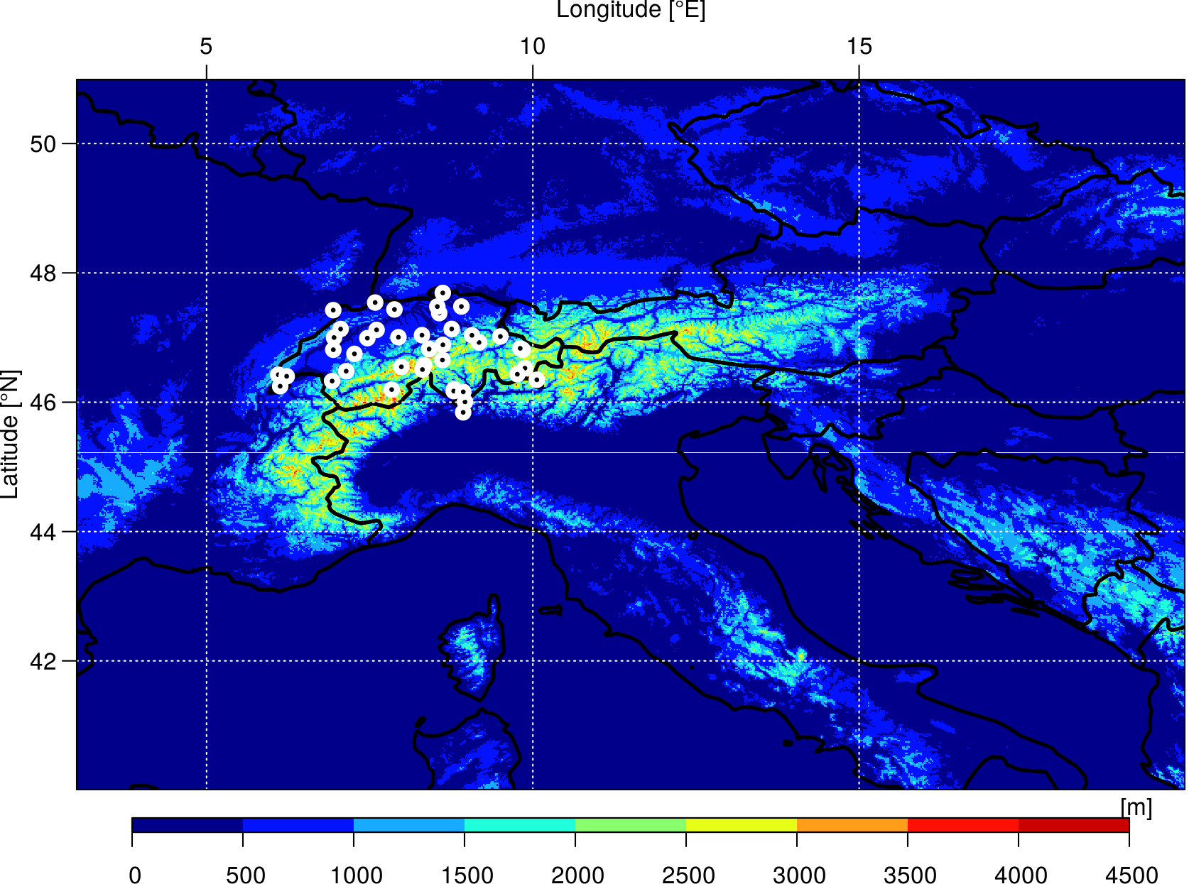
Figure 1Geographical area considered in this study, with ground elevation represented by colours and ground-based stations by white dots.
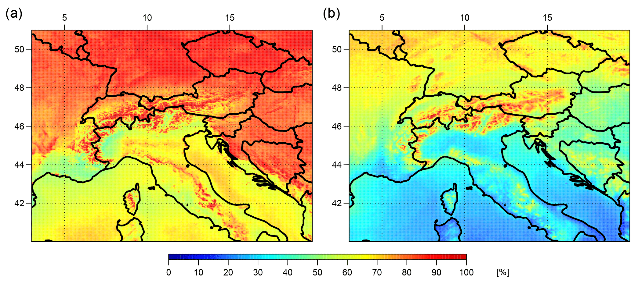
Figure 2Winter (December, January, February) (a) and summer (June, July, August) (b) averaged cloud occurrences in the MODIS-Aqua L3U data set, years 2003–2014.
The increase of cloud cover with altitude is confirmed independently of the instrument or of the time period considered (Fig. 3). There is a slightly different relationship between ground altitude and cloud occurrence in the two data sets due to their different spatial resolution. In very high areas, the cloud cover is constantly overestimated (it often reaches values larger than 80 % of cloud occurrence) regardless of the season, whereas in lowlands the values found are more consistent and lower in summer than in winter, which is also observed in a satellite and ground-based instruments intercomparison by Fontana et al. (2013)
In Fig. 3, different clusters of points can be observed in winter (two clusters) and in summer (three): they are caused by natural variations of cloud amounts with latitude. The low-occurrence group of points in winter (Fig. 3a, c, e) corresponds to cloud occurrences of satellite pixels above sea and above lowlands south of the Alps (approximately below 46∘ N), whilst the high-occurrence group contains pixels north of the Massif Central in France, north of the Alps, and north of the Dinaric Alps in eastern Europe. In summer (Fig. 3b, d, f), cloud amounts get lower, and three groups can be identified: the lower one, as in winter, corresponds to pixels above sea or south of the Alps; the middle one contains pixels above lowlands between roughly 46 and 48∘ N (between the Massif Central and the Alps, and between the Alps and the Dinaric Alps); and the upper group is above lowlands north of the Alps (over 48∘ N). Winter retrievals of AVHRR-PM in 2003–2014 (Fig. 3c) have lower cloud occurrences (approx. −3 %) than those of AVHRR-PM 1982–2002 (Fig. 3e). As discussed later, the satellite's orbital drift might have had an impact on the values.
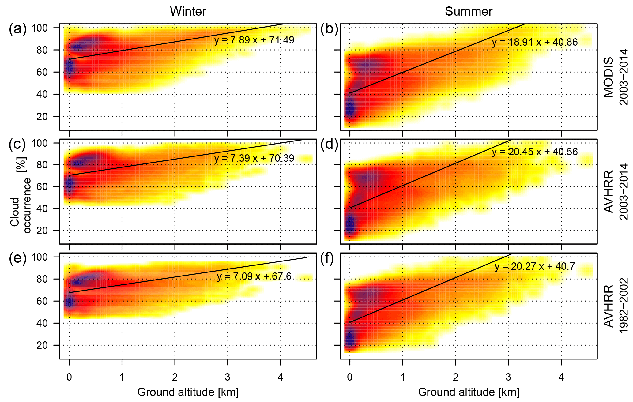
Figure 3Winter (a, c, e) and summer (b, d, f) cloud occurrences for each pixel in the Alps (area shown in Fig. 2) for MODIS-Aqua in 2003–2014 (a, b), AVHRR-PM in 2003–2014 (c, d) and the first part of the AVHRR-PM record (1982–2002; e, f). Colours indicate the density of points (the darker it is, the more points there are). A linear regression is drawn and written on each subfigure to illustrate the overall observed relationship between ground altitude and cloud occurrence.
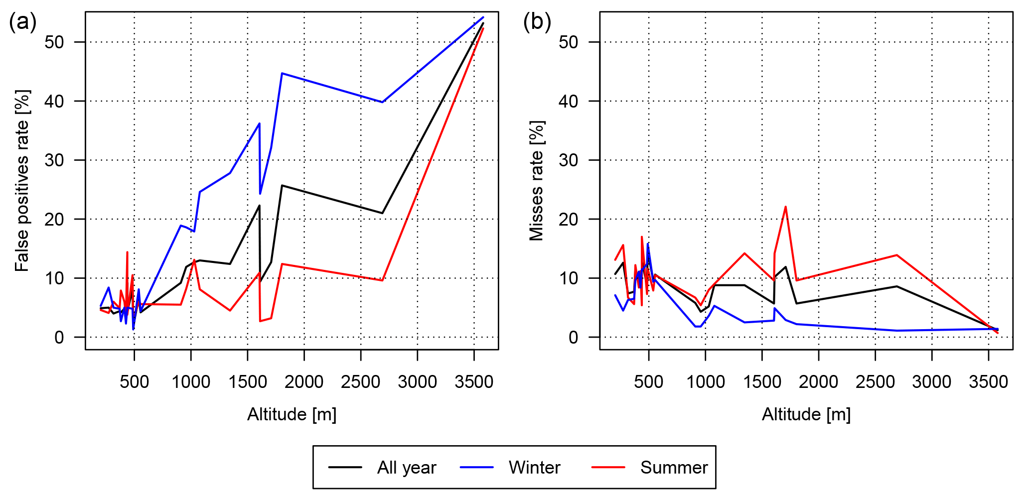
Figure 4MODIS-Aqua cloud mask compared to 24 SYNOP stations in Switzerland. The SYNOP–MODIS overlap varies from one station to another, from 3.3 years to the whole MODIS record (12 years). The satellite mask false positives (a) correspond to when the satellite data set contains a cloud, but the ground observer reports a value of less than 4 oktas of clouds. The misses (b) are the opposite disagreement between the two.
When comparing the cloud mask of MODIS-Aqua to SYNOP observations (Fig. 4), extreme values are seen at the Jungfraujoch station (3580 m a.s.l.), where clouds are reported 98 % of the time in the satellites data sets, corresponding to a 53 % rate of false positives. This rate (Fig. 4a) indeed increases with altitude, more drastically in winter and consistently with the spatial pattern observed before. Night satellite measurements are not exempt from these overestimations, although fewer SYNOP data are available as a reference (elevated stations are not manned at night). The decrease of the miss rate with altitude (Fig. 4b), especially in winter, is directly related to the high overestimation rate at these locations. Except for that, the miss rate observed is relatively steady with altitude. It shows a systematic bias of 5–10 %, most likely caused by the different geometries involved in the comparison. For instance, ground observers might see much further than the boundary of the satellite pixel in which they stand, especially in locations without surrounding relief blocking the view. Considering also the limitations detailed in Sect. 2.2, the cloud masks are overall considered as agreeing under 1000 m.
These results suggest that the presence of snow on the ground, in winter and in summer at high-altitude locations, tricks the satellite retrieval algorithm into detecting more clouds than it should. This is consistent with the appendix of Stengel et al. (2017a), which mentions that the known limitations of these satellite data sets include “shortcomings in cloud detection and optical property retrievals in regions with high surface reflection of solar radiation”. Snow reflectance leads to top-of-atmosphere radiances very similar to water and/or ice clouds in different channels. Some methods can be used to help distinguish between them (see for instance Musial et al., 2014). A widely used solution is to complement spectral data with ancillary data: CC4CL, the retrieval producing the satellite data sets shown here, is indeed based on the snow mask of ERA-Interim. However, given the issues observed here, the spatial resolution (0.7∘ lat–long in ERA-Interim, much lower than that of the satellite products: MODIS-Aqua is 0.02∘ lat–long and AVHRR 0.05∘ lat–long), the quality or the use of the ancillary data might be insufficient.
2.4 Satellite cloud properties
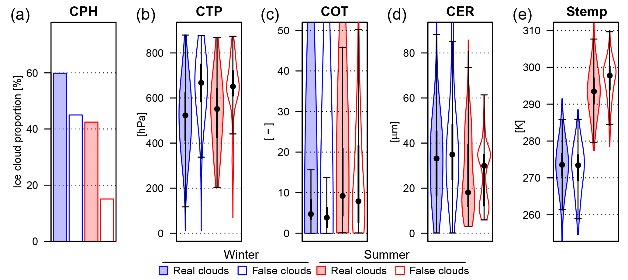
Figure 5Distributions of values of five cloud properties (phase (CPH), top pressure (CTP), optical thickness (COT), effective radius (CER), surface temperature (stemp)) retrieved from MODIS-Aqua in winter and summer at nine stations located above 1000 m of altitude, for actual clouds and falsely detected ones (using SYNOP observations as a reference).
As the cloud property retrieval from satellite-measured radiances is run after the cloud mask computation by the artificial neural networks, any mistake at this first stage carries on to the next. Attempting to retrieve cloud properties in the absence of cloud would lead to unreasonable values. For instance, false clouds are more often of liquid phase than ice (Fig. 5a), are significantly closer to the ground (higher top pressure, Fig. 5b), have lower cloud optical thickness but higher cloud effective radius (Fig. 5c and d), and have higher surface temperatures (Fig. 5e). A surprisingly high mode can also be seen in the effective radius distribution (Fig. 5d) of false clouds in summer, corresponding supposedly to ice particles. These observations are consistent with a retrieval influenced by the presence of snow: these false clouds are lower, warmer, and with larger particles than actual clouds. In summary, cloud mask errors have an important impact on the retrieved cloud properties as well, and identifying such cases before any in-depth analysis is very important.
The previous section presented briefly how the CC4CL satellite retrieval overestimates cloud amounts above elevated areas. The next two sections propose a solution to handle this issue: first, a new binary cloud mask is defined. The combination of several ground-based observations provides insight about the cloud cover at 41 locations in Switzerland. This allows the use of a higher number of locations than the SYNOP stations, especially with more data in elevated areas and without potential issues regarding the subjectivity of SYNOP observations. Subsequently, this cloud mask is used as a reference to train a model for the automated detection of false clouds in the satellite data sets.
3.1 Ground-based data
Downwelling longwave and shortwave radiation as well as ground-based 2 m air temperatures are used in this study to get an estimation of the local cloud cover. Longwave and shortwave downwelling radiation is measured by pyrgeometers and pyranometers, respectively, which consist of a thermopile sensor and a temperature sensor under a small dome. The pyrgeometer's spectral band is 4.5–42 µm, whereas the pyranometer's is 0.3–3 µm. Both instruments have a field of view close to an ideal 180∘ (the exact values depend on the instrument's quality), and each measurement is weighted by the cosine of the incidence angle, giving more importance to radiation at angles close to the zenith.
All measurements were converted to 10 min averages. Information about the measurement setup and data preprocessing can be found in the work by Dürr and Philipona (2004). Of the 41 stations used in this study, 37 are part of the SwissMetNet network (Suter et al., 2006) operated by the Swiss weather office MeteoSwiss, and 4 are part of the Alpine Surface Radiation Budget (ASRB) network (Marty et al., 2002). The pyrgeometers used in the SwissMetNet network are of type CG4 and CGR4 from Kipp & Zonen, with a declared uncertainty of 3 %. Older measurements from the ASRB network have been taken by modified Eppley PIR pyrgeometers, which have an observed uncertainty of 3 W m−2 (Marty et al., 2002). The pyranometers are mostly CM21 from Kipp & Zonen (2 % uncertainty) and a few SPN1 from Delta-T (5 % or 10 W m−2). A detailed list of stations including operation times can be found in Table A1 in the Appendix.
3.2 Topographic data
Topographic information comes from the freely available global digital elevation model (GDEM) Advanced Spaceborne Thermal Emission and Reflection Radiometer (ASTER) version 2 (Tachikawa et al., 2011; ASTER GDEM is a product of METI and NASA). This GDEM has a spatial resolution of 1 arcsec (approximately 30 m at the Equator).
3.3 Method for the ground-based cloud mask
The method described here combines two different types of radiation to estimate the state of the sky at 41 locations, with a 10 min temporal resolution.
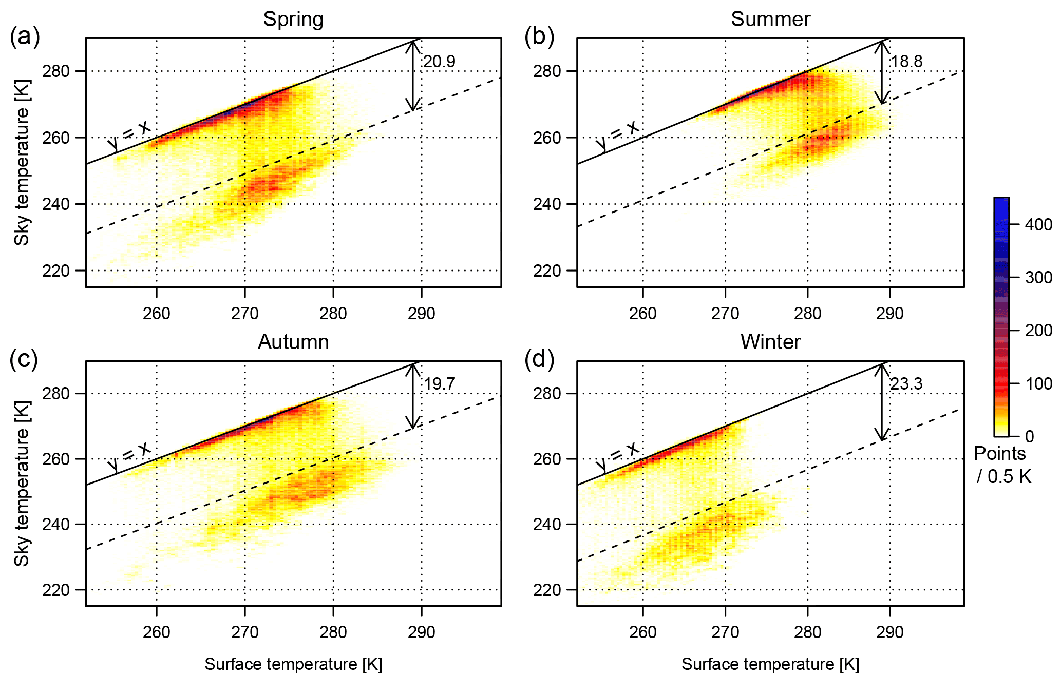
Figure 6Comparison of daytime sky and ground temperatures at Weissfluhjoch station (2690 m) in Switzerland, per season, using data from 1994 to 2010. The upper cluster corresponds to in-cloud and overcast conditions, whilst the lower one corresponds to clear-sky times. The points in between are partially cloudy conditions. The dashed line corresponds to the automatically detected threshold under which values are considered as being part of the lower cluster.
Ground-based longwave measurements have been used in various ways to estimate cloud cover (Dupont et al., 2008; Dürr and Philipona, 2004; Viúdez-Mora et al., 2009). The method used here is inspired by the work of Herrmann et al. (2015) and consists in converting downwelling longwave measurements (L, W m−2) into estimated sky temperatures (Tsky, K) and then comparing them to ground-based (2 m) temperatures. As the radiation emitted by a cloud is comparable to that of a black body at the same temperature, the Stefan–Boltzmann law is used for the conversion:
where σ is the Stefan–Boltzmann constant ( W m−2 K−4) and the atmospheric emissivity ϵ is approximated to unity.
Figure 6 shows cluster plots of the estimated sky temperature versus the measured ground temperature. Clear-sky estimates always cluster at low temperatures (being a mixture of atmospheric and cosmic background temperatures), whereas cloud base temperatures are significantly higher (representative of tropospheric temperatures at the cloud height). Scattered cloud conditions are characterised by values falling between the two main clusters.
The detection of the lower cluster border is done in five steps. First, the differences between ground and sky temperatures are calculated. Then, the density distribution of these values is computed (black curve in Fig. 7) and smoothed (red curve). One way to find the cluster border is to look for a strong density increase in this distribution, so in the third step the derivative (blue curve in Fig. 7) is computed. As the upper cluster is spread over several degrees kelvin, only temperature differences larger than 5 K can correspond to the lower cluster. The fourth step consists in looking for the maximum of the derivative for differences over 5 K. Lastly, the cluster border is set at the minimal temperature difference so that half this maximum is reached (yellow vertical line in Fig. 7). The sensitivity of this value was analysed and showed that a change of ±20 % had a very limited impact on the size of the lower cluster. It did not have a significant effect on the correlation of the resulting cloud mask with SYNOP observations either.
Due to the daily temperature cycle, days and nights are clustered separately to ensure that accurate lower cluster limits are obtained. Local sunrise and sunset times are used as time limits.
Different applications of this method are shown in Fig. 7, for daytime conditions in winter and summer. One station with a long data record (Weissfluhjoch, 16 years) is compared to another one with a very short record (Segl-Maria, 1 year). As can be seen, the main advantage of detecting the cluster's border as a strong density increase is the excellent adaptability to different amounts of data as well as to different cluster shapes.
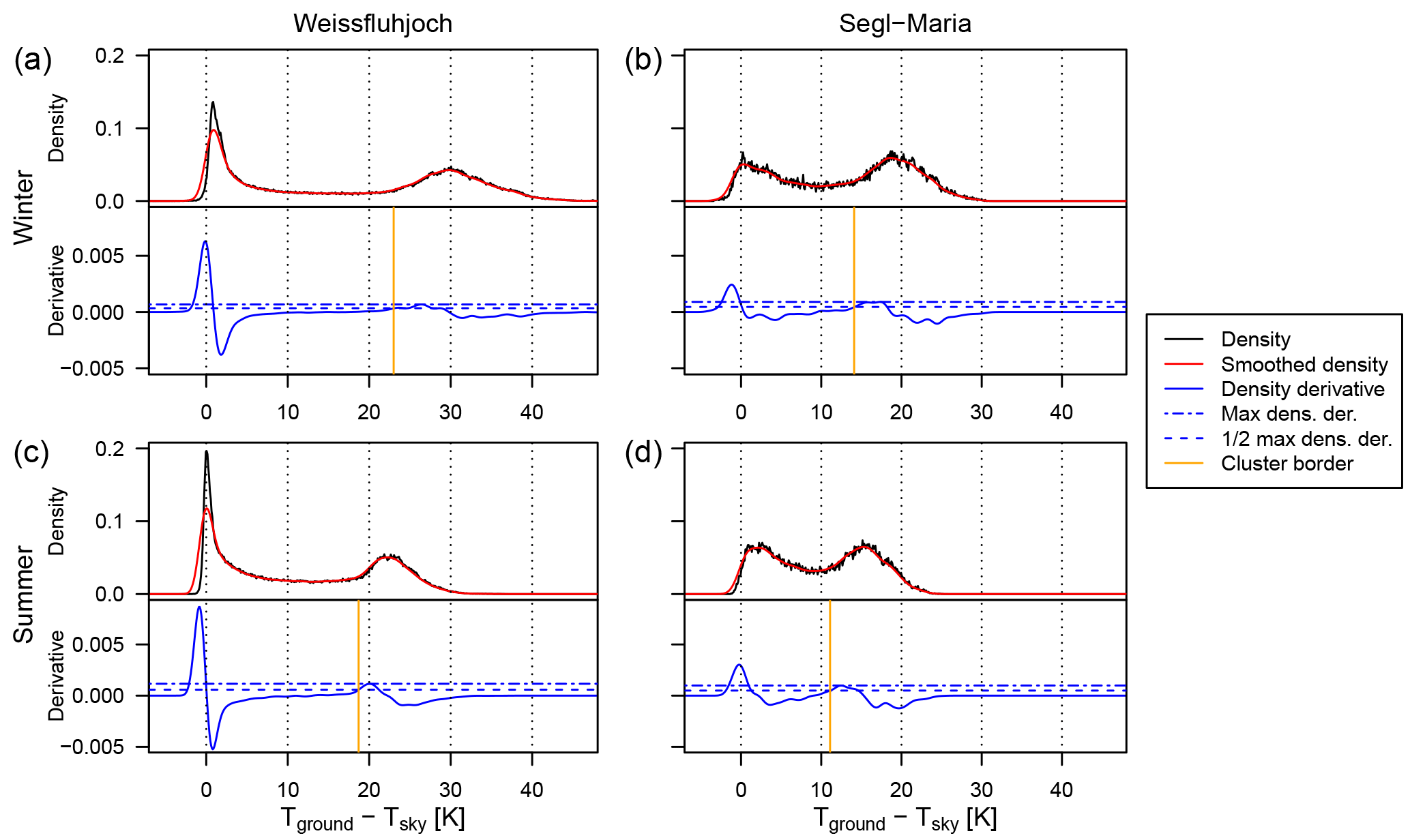
Figure 7Detection of the longwave lower cluster on daytime data, at two different stations (a, b: Weissfluhjoch; b, d: Segl-Maria; 1 year of measurements), for winter (a, b) and summer (c, d) seasons.
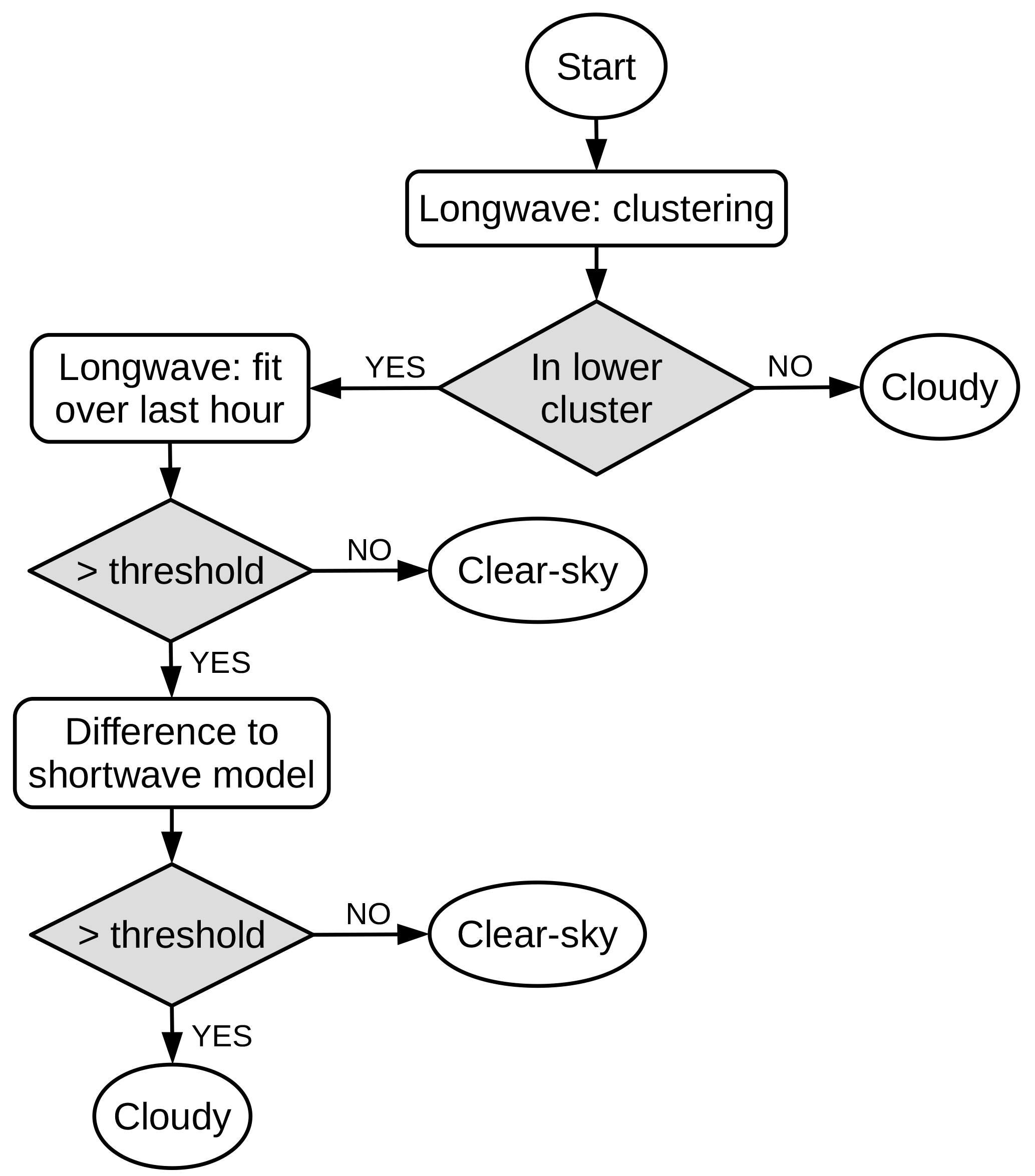
After this clustering step, two other criteria are combined to discriminate partially cloudy conditions from clear-sky ones (Fig. 8). The stability of the longwave measurements over the preceding hour is used as a sign of partial cloud cover, as in Dürr and Philipona (2004). However, a cloud is detected only if this criterion reaches a given threshold at the same time as the difference between estimated and measured shortwave radiation exceeds another threshold. Exploration of the parameter space in 2-D has shown that this second criterion improves the classification and that the threshold values are not particularly sensitive. The stability of the longwave measurements over the preceding hour is computed as the root-mean-square deviation between the values and a linear fit applied to them (the threshold in the algorithm is set to 1.75 W m−2).
The shortwave criterion C is defined as a weighted sum of relative differences between the measured and estimated global radiation over the preceding hour (the threshold is set to 0.15 and is dimensionless). The weights are larger close to the time of interest t:
where i is a time index varying between 0 and 60 min by steps of 10 min, and Sm, t and Se, t are respectively the measured and estimated global radiation (in W m−2) at time t.
The incoming global radiation Se, t is estimated using a simple model described in Sun et al. (2013), the model SW1 in their paper:
where τ is the atmospheric transmittance (dimensionless), S0 the solar constant (1367 W m−2), dt the Earth–Sun distance (in astronomical units, AU), and θt the solar zenith angle (in radians) at time t. The particularity of this model is that the atmospheric transmittance τ is approximated as a linear function of the altitude, following Tasumi et al. (2000).
The shading effect of topography is taken into account due to its significant effect on radiation in mountainous areas (Lai et al., 2010). The shading angle H is defined as the minimal elevation above horizon required to see the sky above the surroundings. When the Sun is at a given azimuth ϕ, if its elevation is below H(ϕ), then the estimated radiation is set to zero. The shading angles were computed at each station using the ASTER GDEM, taking into account surroundings up to a distance of 0.5∘ lat–long (55 by 38 km at 46∘ N), with a resolution of approximately 1 arcsec (15 by 10 m at 46∘ N).
3.4 Results
The obtained cloud mask was validated against SYNOP observations, with a time difference of at most 10 min. The percentages of misclassified clouds per okta are shown in Fig. 9. The largest source of error comes from the transformation of the SYNOP observation into a binary threshold: it is difficult for the radiation cloud mask algorithm to follow this strict threshold when the distinction between 3 and 4 oktas is quite subjective. The cloud mask is hence accurate 85.4 % of the time, and this value reaches 90.3 % if both clear and cloudy classifications are allowed for 3- and 4-okta observations. With this 1-okta difference allowed, the probability of correctly detecting clouds is 87.6 %, and the probability of false detections is 5.6 %. This is consistent with Fig. 9, because more clear (0–1 okta) and cloudy (7–8 oktas) conditions are recorded than partial ones. A bias of 0.913 okta is present, confirming a tendency to miss some clouds. Thin and high clouds cause only minor perturbations in the radiation measurements compared to the clear-sky conditions and for this reason are more likely to be missed. A higher number of clouds are missed at night due to the lack of shortwave information. However, the negligible difference between false positives between day and night shows that a sparse cloud cover missed by the radiation instruments at night is most likely missed also by the human observer. The results' consistency is good among the different stations (the averaged accuracy is 91±2 %), the lowest accuracy being at the Jungfraujoch (86 %), which is on a mountain pass where clouds can be observed below the observatory.
Even though the accuracy of the cloud mask presented here is limited for partially cloudy cases, these results are of great value for validation when a stable long-term reference is needed, such as in the validation of long-term satellite products. The results further suggest that this method could potentially be used outside the geographical area evaluated here, as the clustering method should adapt automatically to different climatic conditions.
In this last section, a model is trained to automatically detect false positives in the satellite data sets. Using the radiation cloud mask as a reference, this model combines several variables retrieved from satellite-measured radiances with information about the topography and time of the retrieval. The possibility of using the model at other times than those used for training is considered, and the model is applied to long satellite time series. Similarly, its ability to extrapolate to other locations than where it was trained is evaluated, and maps of its effects are discussed.
4.1 Methods
A decision tree was trained to automate the identification of false clouds in the satellite data sets. The model's inputs are the five variables retrieved from the satellite radiances by the CC4CL algorithm (cloud phase, cloud optical thickness, cloud top pressure, cloud effective radius, and surface temperature), as well as the ground altitude, the standard deviation of the surrounding ground altitudes, and a time variable. Time is represented as a sinusoidal function with a period of 1 year, peaking on 15 January (+1) and on 15 July (−1). The standard deviation of the surroundings is computed within a radius of 3 km on the 30 m GDEM. Using these variables, the model predicts if the sky actually contains a cloud or not. The radiation cloud mask defined in Sect. 3 is used as a reference for training. The training is done by 10-fold cross-validation with random sampling, using recursive partitioning as presented in Breiman (1984). Testing metrics are computed over the 10 models obtained, and only the best one is then validated against SYNOP observations. After this validation, the structure of the model is discussed and some groups of points are defined. Focusing on these groups allows analysing the whole dimension space without considering each cloud property or each point one by one. The performance of the model is tested on each of these groups, and this permits the identification of some potential weaknesses.
Once validated, the decision tree is applied to the two satellite data sets presented at the beginning of this study. First, the effect of the model on time series of cloud properties is discussed. Then, leave-one-out validation is done to assess if the model can be applied at locations where it was not trained and what kind of results can be expected in these circumstances. Leave-one-out validation consists in training several models, each with a training set composed of all but one station. Testing is done on this last station, and all the testing results are regrouped. Important information about the model weaknesses can be deduced from where the model had difficulties to adapt without training. It provides an overall idea about how the model will perform at locations where no reference data are available. Once this is done, the model is applied to a larger geographical area and the results are discussed as another insight on the model's strengths and weaknesses.
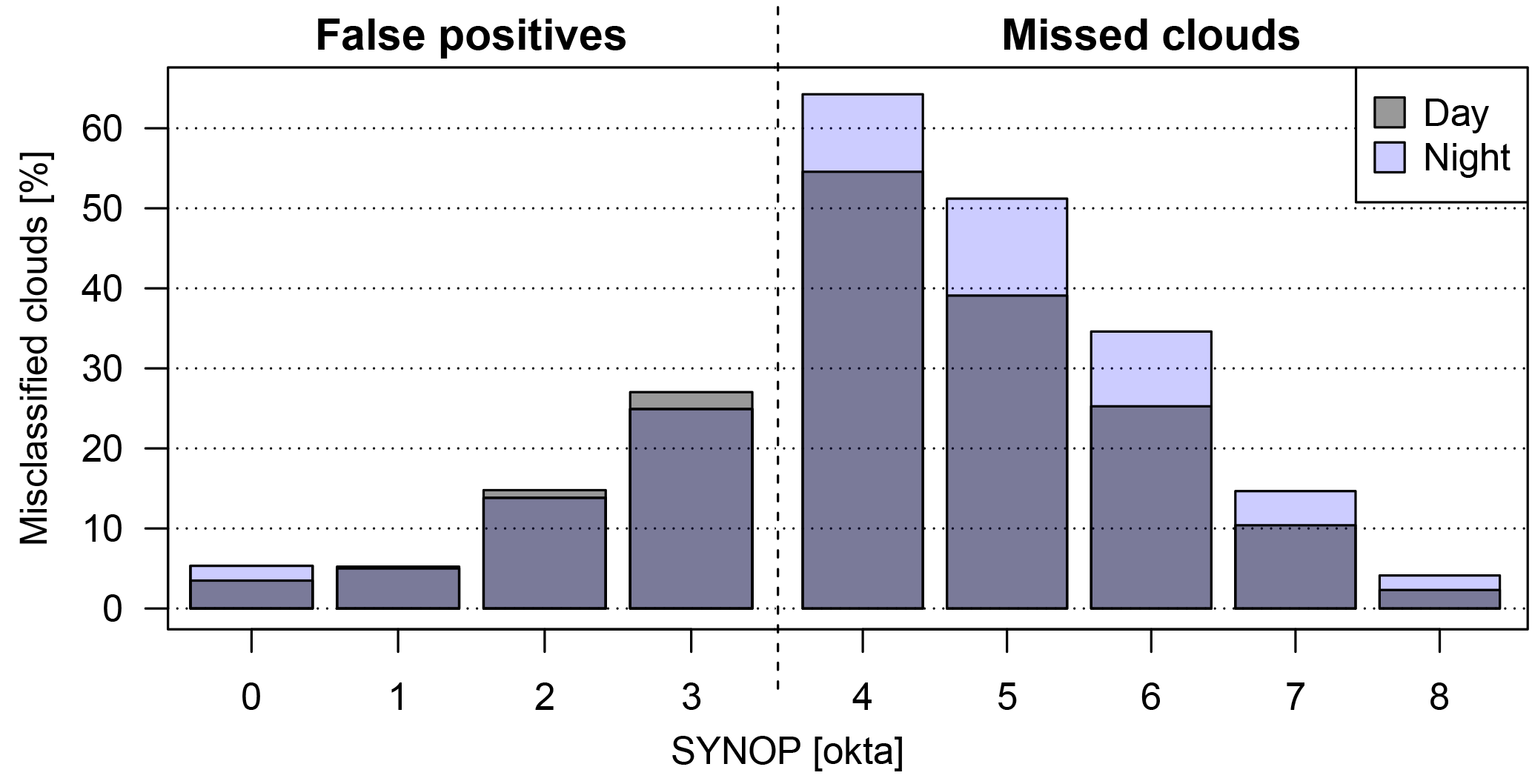
Figure 9Distribution of the ground-based cloud mask errors as a function of SYNOP observations at 21 stations. The vertical dashed line represents the binary threshold applied to the SYNOP observations.
4.2 Analysis and validation of the model
The model obtained at the end of the training process is a large decision tree drawn in Fig. 10. After the overall results are reviewed, the groups of points circled in this figure are analysed more in detail.
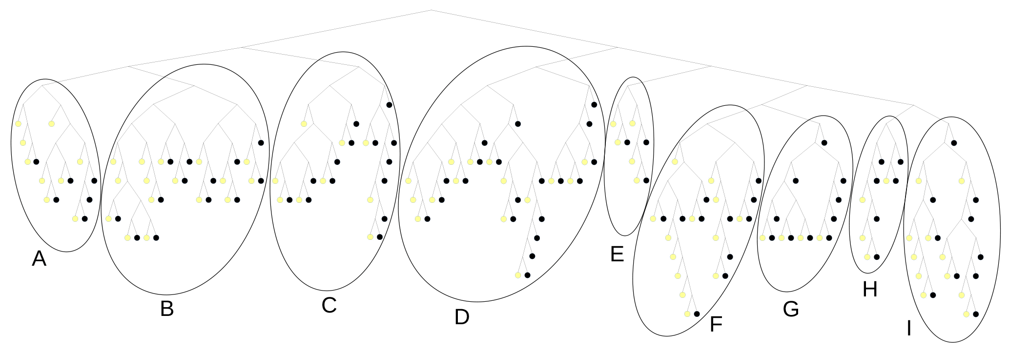
Figure 10Structure of the model. Small circles correspond to the tree final nodes (also called leaves): light ones are classified as clear sky, and dark ones as cloudy. The parts circled and labelled with letters correspond to the groups of points defined in Table 2.
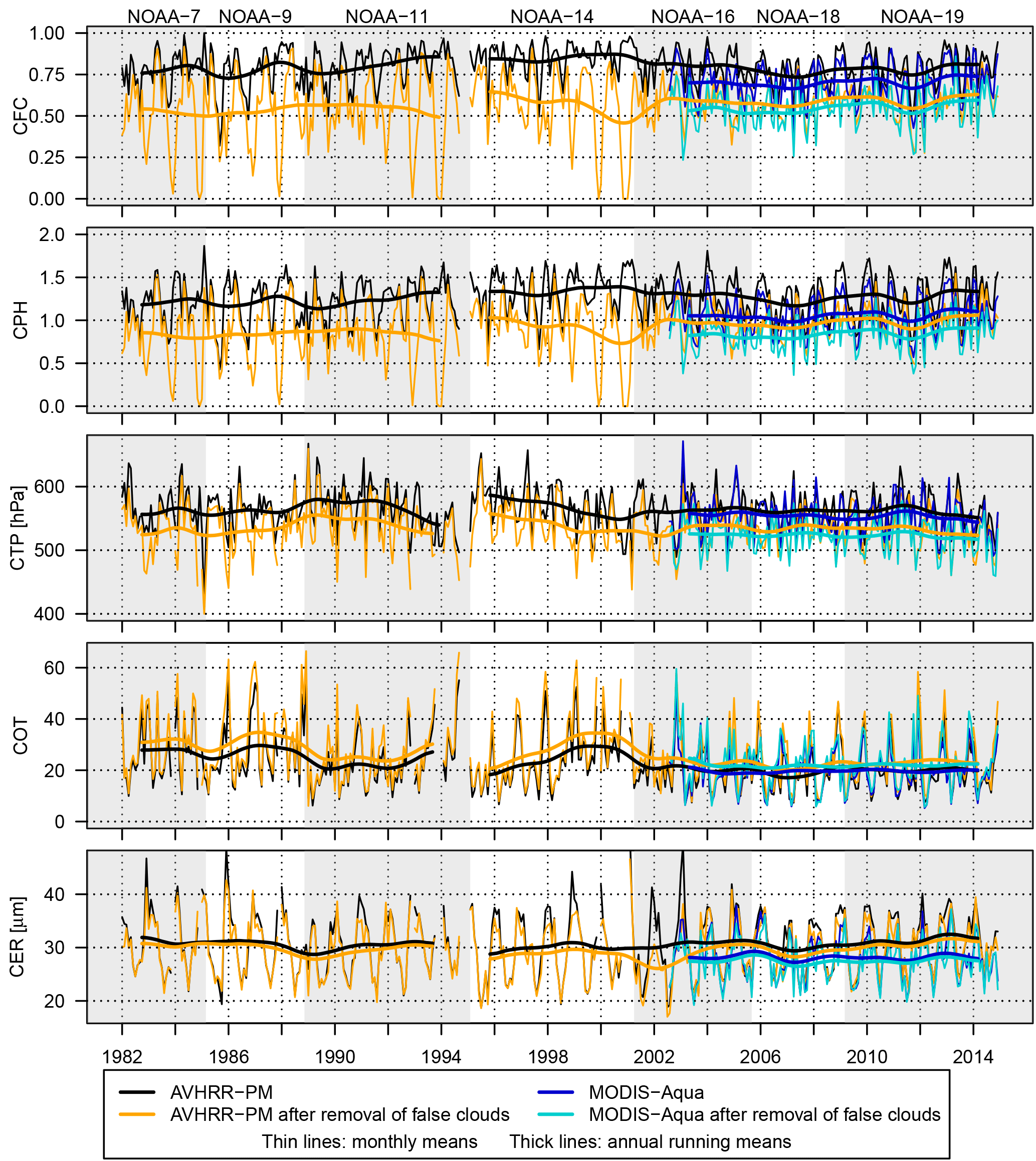
Figure 11Time series of monthly means (thin lines) and annual moving averages (thick lines) of cloud properties, before and after removing points flagged by the model as potential false positives. Nine SYNOP stations located above 1000 m are averaged together. CFC stands for cloud fractional cover, CPH for cloud phase (0: no cloud; 1: liquid phase; 2: ice phase), CTP for cloud top pressure, COT for cloud optical thickness, and CER for cloud effective radius.
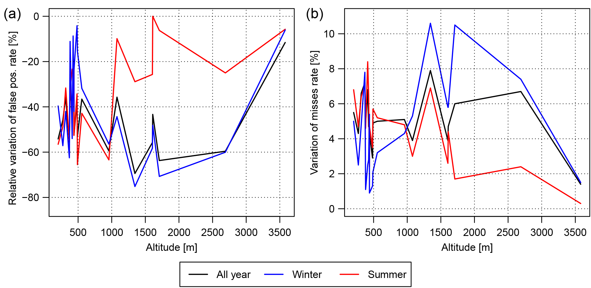
Figure 12For each SYNOP station, a model was trained at all stations except one (leave-one-out validation). The figure shows the effect each model had on the rates of false positives (a, relative percentages) and missing clouds (b, absolute percentages) at the station left out, using SYNOP observations as a reference.

Figure 13Effect of the model on cloud occurrences, in percent relative to the initial cloud occurrences. The results are averaged over MODIS-Aqua data set (2003–2014) by season: winter (a), spring (b), summer (c), and autumn (d). The seasons are defined as December, January, and February; March, April, and May; June, July, and August; September, October, and November.
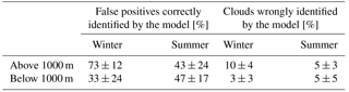
Overall, the test metrics give a 82.6 % probability of detecting false positives and a 10.9 % probability of false detections. They are computed using the radiation cloud mask as a reference and averaged over the 10 tests of the cross-validation. When validated against SYNOP observations, results show that in winter above elevated areas, where most of the satellite false cloud detections happen, 73±12 % of errors are identified (Table 1). The amount of missing clouds in these conditions is increased by 10±4 %, whereas lower values are found in all other conditions. In summer, around 45 % of the overestimations are detected, with quite large differences between the stations but with no significant link to the station's altitude. Globally, 62±13 % of the cloud mask overestimations are detected, reducing the systematic false-positive error from 14.4±15.5 to 4.3±2.8 % but increasing the missed clouds from 8.7±3.5 to 15.6±2.1 %. Although it might seem like this proposed correction only shifts the problem (from false clouds to missing clouds), this is not the case: the reduction of false positives is associated with a reduction of their uncertainty (±15.5 to ±2.8). This means that the distribution of false positives is more homogeneous than before and, thus, that the difference between high areas and lower ones has been reduced. Moreover, the increase (+7 %) of missed clouds is global and does not correspond to a simple shift of the problem in elevated areas.
Table 1Evaluation of the model's effects on MODIS data set using SYNOP data as a reference at 20 SYNOP locations (7 above 1000 m, 13 below; 4 stations with limited overlap between SYNOP and the ground-based radiation measurements were excluded). The two left columns contain the percentage of false positives in the satellite data that were correctly identified by the model. The two right ones contain the percentage of clouds identified in the satellite data which are considered false by the model, even though they are actual clouds according to SYNOP observations with the binary threshold applied.
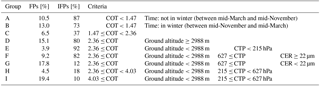
As proposed in Fig. 10, groups of points can be delineated in the tree and are characterised by the criteria detailed in Table 2. All of these groups are separated in subgroups that are not described here. As can be seen in the table, COT is one of the most important variables in this model. Groups A and B, characterised by a small COT and which contain a large amount of well-classified points, most likely also contain a non-negligible amount of cirrus clouds, too thin to be seen by the reference cloud mask produced in this study. Group D is the only one containing only clouds located above mountains, and its high detection percentage confirms the efficiency of the model. Groups C, G, H, and I are all characterised by low model performance. Group C can be understood as a small group of points scattered in the dimension space and which did not trigger a particular response of the model. The others are mainly composed of large COT, and group G probably corresponds to liquid phase clouds (CTP under 627 hPa and CER under 22 µm).
As can be observed, groups of points that seem related (for instance, F and G) can be understood very differently by the model, which suggests that a more complex model could be necessary to catch subtle differences between false and real clouds, and to improve the results.
Table 2Main branches of the tree. The letters in the first column correspond to the groups circled in Fig. 10. The second column states the amount of false positives (FPs) in the satellite data falling into each branch; the third one states how many of them were correctly identified by the model (IFPs: identified false positives). The remaining columns describe the parameters and thresholds leading to each branch. COT: cloud optical thickness; CTP: cloud top pressure; CER: cloud effective radius.
4.3 Result of filtering the satellite data set using the decision tree model
Having looked at the limitations of the model and at the expected results, the decision tree was then applied to the satellite-derived cloud property time series. The pixels corresponding to nine stations above 1000 m were extracted from the satellite data set, and false clouds were detected and removed using the decision tree. The main cloud properties were observed before and after removal of these false positives and are averaged per year and per month in Fig. 11. Although the model is trained on the MODIS-Aqua data set only (2003–2014), a temporal extrapolation is attempted to the whole NOAA AVHRR-PM time series (1982–2014).
After removal of the points identified by the model as likely not to be clouds, the cloud fractional cover (CFC) is lower. As expected, the points removed were greater in number in winter than in summer, were at higher altitudes, and had larger optical thickness and smaller effective radius. This is highly consistent with the changes observed when removing from MODIS-Aqua data set the clouds not observed by a human observer (Fig. 5). The difference between MODIS-Aqua and the MODIS-Aqua corrected time series seems constant over time and suggests that the effects of the model are temporally consistent. Over the years 2003–2014 the two satellite data sets agree very well, except for a small offset caused by the difference of spatial resolutions. Since the AVHRR series used here is not homogenised regarding e.g. drifts in overpass time between different NOAA satellites (Stengel et al., 2017a), its behaviour is not stable over time. This can be seen over the years 1982–2002, near the end of each NOAA satellite, where values diverge progressively from their average. Some of these values are not expected by the model and tend to be removed, causing very low CFC values for several winters (at the end of 1983, 1984, 1987, etc.). As the satellites were drifting in time (up to 3 h and 30 min for NOAA 11), this suggests the need to first correct the cloud properties for the cloud diurnal cycle before applying the decision tree correction.
When compared to the latitude-weighted 60∘ S–60∘ N time series in Stengel et al. (2017a), the time series in Fig. 11 have wider seasonal amplitudes. The satellite's drifting in time also has a larger impact on the values. Both are related to the size of the areas over which the data are averaged. The proportion of cloud ice particles is significantly higher in the time series in Switzerland than in Stengel et al. (2017a), even in low areas (results not shown), and after applying the model. Similarly, the cloud optical thickness is approximately twice as large in the time series presented here as in Stengel et al. (2017a). The cloud effective radius decrease from mid-2001 to mid-2003 is due to the change of channel on NOAA-16 (Heidinger et al., 2014) and can be observed in Stengel et al. (2017a) as an increase of effective radius. The channel 3.7 µm was switched to 1.6 µm, which seems to trigger the model. For this same property, a bias can be observed on values retrieved from NOAA-19, which seem to have an increasing difference with MODIS-Aqua. This can also be seen in Stengel et al. (2017a) and might be an instrumental bias.
4.4 Leave-one-out validation
The leave-one-out validation results in Fig. 12 suggest that the model can reliably be generalised in space, especially for elevated areas in winter. The highest station of the data set (Jungfraujoch) is an extreme case in this data set and cannot be well understood by the model if it is not part of the training set. Although good, the performance above elevated areas is lower in this validation than the values obtained previously on a slightly larger data set (Table 1, errors correctly identified above 1000 m). This suggests that increasing the amount of stations would be beneficial. However, even without increasing the number of stations, significant results (more than 50 % of the satellite cloud mask overestimations identified) can still be expected.
In this Fig. 12, one can also observe that the detection of false positives in the satellite data is less efficient above elevated areas in summer, whereas in lower areas there is no significant seasonal difference. This might be a sign that seasonal differences in mountains are not fully understood by the model, probably due to the lower number of stations above 1000 m than below. As winters contain a much higher number of false positives than summers, false positives in summer at high altitudes end up being poorly represented in the data set. Using a probabilistic approach taking into account the different amount of points in each condition might help reduce the model's skewness in favour of the detection of the most recurring problems.
No link seems to exist between the ability of the model to generalise to a station and the complexity of the station's surrounding, suggesting that the model already gets the most out of this variable. For stations below 1000 m, a moderate negative correlation (−0.46) was found between the average relative increase of missing clouds caused by the model and the distance between a station and the centre of its corresponding satellite pixel. A similar correlation (−0.43) was observed between this distance and the ability of the model to detect false positives in winter. This suggests that lower performance is partially caused by a spatial offset between the satellite viewing scene and the ground-based one. A solution out of the scope of this study would be to look more in detail into the satellite viewing geometry of the comparison scenes, and maybe to combine several satellite pixels in a weighted mean for comparison with a ground-based station.
4.5 Larger-scale model application
Lastly, the model was applied in a large area, and maps of the effect on the cloud coverage were produced (Fig. 13). They confirm that, even at locations outside the training data, the model reduces cloud occurrences to more reasonable values above elevated areas, especially in winter (Fig. 13a). The systematic removal of 7 % of the clouds (identified as false positives even though they were most likely real clouds) is not restricted to a specific area.
With a training set made of stations located only in Switzerland, the results appear very consistent above land also outside this area. Considering the model output over a wider area however illustrates its limitations, mainly over sea and lakes in every season apart from winter. Especially in summer, clouds are detected as false positives over water bodies, as their surface temperature is lower than that of the surrounding land. For instance, a blue spot can be seen in the Po Valley of northern Italy (approx. 45.2∘ N, 8.5∘ E), where rice cultures are flooded during summer months, which significantly lowers the surface temperature. This confirms the importance that the model gives to the surface temperature and suggests that either the model should be applied only over land or it should be aware of the land–sea difference (for instance, adding a land–sea mask would be an easy step, but finding radiation measurements above sea for training might be difficult).
As applying a decision tree on data is a very quick process, this model is a simple solution to remove a significant amount of issues over elevated areas, at the reasonable cost of slightly and homogeneously decreasing the amount of clouds.
Two satellite data sets of ESA's CCI on clouds were seen to overestimate the cloud cover above elevated areas. MODIS-Aqua and AVHRR-PM can contain false cloud detection rates up to 54 % in winter in mountainous areas (above ground with an elevation higher than 1000 m). These cloud mask errors also have an important impact on the cloud properties, as retrievals on missing clouds often have unexpected values. Identifying them prior to any detailed analysis is a necessary step.
Using longwave and shortwave radiation measurements at 41 stations in Switzerland, a binary cloud mask was defined. It is tailored to each station and each season thanks to a simple automated clustering of the longwave data. Shortwave data and a second longwave criterion are then used to provide more insight in partially cloudy cases. Validation against SYNOP shows that the model has an 87.6 % probability of detecting cloudy skies using this combination of ground-based information and a 5.6 % probability of false detections.
This ground-based cloud mask was then used as a reference to train a model for the detection of false clouds in the satellite data sets. The model's input contains variables such as the satellite-retrieved cloud properties, as well as ground and time information. In the Swiss Alpine region, the use of the decision tree model as a quality filter permitted the rejection of 62 % of the false cloud detections in the satellite cloud property data set, with the limitation of causing the removal of 7 % of real clouds in the process. This made a significant improvement to the quality of the satellite cloud property data set over this area. These results are interesting for any application where one can afford to reduce the amount of data in order to increase its quality. Improved results might be obtained by using a probabilistic approach, likely to allow under-represented categories to be better understood. A higher number of elevated stations could also be beneficial. Expanding the study area to other latitudes using either already-computed cloud masks or data from the worldwide Baseline Surface Radiation Network (Ohmura et al., 1998), for instance, would be an expected follow-up.
Considering how time- and resources-consuming the computation of large satellite data sets is, fast post-processing algorithms such as the one proposed in this study are likely to be interesting solutions as more and more data become available. Moreover, as demonstrated here, having several data sets produced by the same retrieval algorithm is a great asset as it allows them to be post-processed in the same manner.
The satellite data used in this study were obtained from the Cloud_cci project group and can be accessed via the data download portal linked to the data set DOI (Stengel et al., 2017b, c). The ground-based data were obtained from MeteoSwiss via the IDAWEB portal (https://gate.meteoswiss.ch/idaweb, last access: July 2017), which grants “a direct cost-free access to archive data of MeteoSwiss ground-level monitoring networks [...] to users in the field of teaching and research”.
Table A1Location and data coverage of the 41 ground-based stations used in this study. The length of overlap with MODIS is not specified when the whole record overlaps temporally with the MODIS time range (1 August 2002 to 31 December 2014).
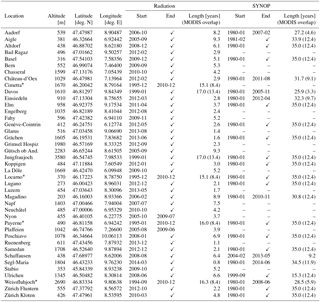
* Radiation data from the ASRB network. If not specified, radiation data are from MeteoSwiss. All SYNOP observations are from MeteoSwiss.
✓End date of the ground-based record is after the end of the satellite records
(31 December 2014).
The authors declare that they have no conflict of interest.
This work was funded by the European Space Agency within the framework of the
Climate Change Initiative. Most of the work was carried out at ECSAT (ESA).
We would like to thank MeteoSwiss for providing the radiation and synoptic
data, and the scientists of the Remote Sensing Group at Rutherford Appleton
Laboratory for their support and advice.
Edited by: Mark Kulie
Reviewed by: two anonymous referees
Barbaro, S., Cannata, G., Coppolino, S., Leone, C., and Sinagra, E.: Correlation between relative sunshine and state of the sky, Sol. Energy, 26, 537–550, https://doi.org/10.1016/0038-092X(81)90166-3, 1981. a
Barnes, W., Pagano, T., and Salomonson, V.: Prelaunch characteristics of the Moderate Resolution Imaging Spectroradiometer (MODIS) on EOS-AM1, IEEE T. Geosci. Remote, 36, 1088–1100, https://doi.org/10.1109/36.700993, 1998. a
Bojanowski, J., Stöckli, R., Tetzlaff, A., and Kunz, H.: The Impact of Time Difference between Satellite Overpass and Ground Observation on Cloud Cover Performance Statistics, Remote Sens.-Basel, 6, 12866–12884, https://doi.org/10.3390/rs61212866, 2014. a
Breiman, L.: Classification and regression trees, Chapman & Hall/CRC, New York, NY, available at: http://lib.myilibrary.com?id=1043565 (last access: 18 May 2018), 1984. a
Cracknell, A. P.: The advanced very high resolution radiometer (AVHRR), Taylor & Francis, London, Bristol, PA, 1997. a
Davies, R., Jovanovic, V. M., and Moroney, C. M.: Cloud heights measured by MISR from 2000 to 2015, J. Geophys. Res.-Atmos., 122, 3975–3986, https://doi.org/10.1002/2017JD026456, 2017. a
Dee, D. P., Uppala, S. M., Simmons, A. J., Berrisford, P., Poli, P., Kobayashi, S., Andrae, U., Balmaseda, M. A., Balsamo, G., Bauer, P., Bechtold, P., Beljaars, A. C. M., van de Berg, L., Bidlot, J., Bormann, N., Delsol, C., Dragani, R., Fuentes, M., Geer, A. J., Haimberger, L., Healy, S. B., Hersbach, H., Hólm, E. V., Isaksen, L., Kållberg, P., Köhler, M., Matricardi, M., McNally, A. P., Monge-Sanz, B. M., Morcrette, J.-J., Park, B.-K., Peubey, C., de Rosnay, P., Tavolato, C., Thépaut, J.-N., and Vitart, F.: The ERA-Interim reanalysis: configuration and performance of the data assimilation system, Q. J. Roy. Meteor. Soc., 137, 553–597, https://doi.org/10.1002/qj.828, 2011. a
Dupont, J.-C., Haeffelin, M., and Long, C. N.: Evaluation of cloudless-sky periods detected by shortwave and longwave algorithms using lidar measurements, Geophys. Res. Lett., 35, L10815, https://doi.org/10.1029/2008GL033658, 2008. a
Dürr, B. and Philipona, R.: Automatic cloud amount detection by surface longwave downward radiation measurements, J. Geophys. Res., 109, D05201, https://doi.org/10.1029/2003JD004182, , 2004. a, b, c, d
Fontana, F., Lugrin, D., Seiz, G., Meier, M., and Foppa, N.: Intercomparison of satellite- and ground-based cloud fraction over Switzerland (2000–2012), Atmos. Res., 128, 1–12, https://doi.org/10.1016/j.atmosres.2013.01.013, 2013. a
Heidinger, A. K., Foster, M. J., Walther, A., and Zhao, X. T.: The Pathfinder Atmospheres – Extended AVHRR Climate Dataset, B. Am. Meteorol. Soc., 95, 909–922, https://doi.org/10.1175/BAMS-D-12-00246.1, 2014. a, b
Herrmann, E., Weingartner, E., Henne, S., Vuilleumier, L., Bukowiecki, N., Steinbacher, M., Conen, F., Collaud Coen, M., Hammer, E., Jurányi, Z., Baltensperger, U., and Gysel, M.: Analysis of long-term aerosol size distribution data from Jungfraujoch with emphasis on free tropospheric conditions, cloud influence, and air mass transport, J. Geophys. Res.-Atmos., 120, 9459–9480, https://doi.org/10.1002/2015JD023660, 2015. a, b
Hollmann, R., Merchant, C. J., Saunders, R., Downy, C., Buchwitz, M., Cazenave, A., Chuvieco, E., Defourny, P., de Leeuw, G., Forsberg, R., Holzer-Popp, T., Paul, F., Sandven, S., Sathyendranath, S., van Roozendael, M., and Wagner, W.: The ESA Climate Change Initiative: Satellite Data Records for Essential Climate Variables, B. Am. Meteorol. Soc., 94, 1541–1552, https://doi.org/10.1175/BAMS-D-11-00254.1, 2013. a
Karlsson, K.-G.: A 10 year cloud climatology over Scandinavia derived from NOAA Advanced Very High Resolution Radiometer imagery, Int. J. Climatol., 23, 1023–1044, https://doi.org/10.1002/joc.916, 2003. a
Lai, Y.-J., Chou, M.-D., and Lin, P.-H.: Parameterization of topographic effect on surface solar radiation, J. Geophys. Res., 115, D01104, https://doi.org/10.1029/2009JD012305, , 2010. a
Long, C. N., Ackerman, T. P., Gaustad, K. L., and Cole, J. N. S.: Estimation of fractional sky cover from broadband shortwave radiometer measurements, J. Geophys. Res., 111, D11204, https://doi.org/10.1029/2005JD006475, 2006. a
Malberg, H.: Comparison of Mean Cloud Cover Obtained By Satellite Photographs and Ground-Based Observations Over Europe and the Atlantic, Mon. Weather Rev., 101, 893–897, https://doi.org/10.1175/1520-0493(1973)101<0893:COMCCO>2.3.CO;2, 1973. a
Martínez-Chico, M., Batlles, F., and Bosch, J.: Cloud classification in a mediterranean location using radiation data and sky images, Energy, 36, 4055–4062, https://doi.org/10.1016/j.energy.2011.04.043, 2011. a
Marty, C., Philipona, R., Fröhlich, C., and Ohmura, A.: Altitude dependence of surface radiation fluxes and cloud forcing in the alps: results from the alpine surface radiation budget network, Theor. Appl. Climatol., 72, 137–155, https://doi.org/10.1007/s007040200019, 2002. a, b
McGarragh, G. R., Poulsen, C. A., Thomas, G. E., Povey, A. C., Sus, O., Stapelberg, S., Schlundt, C., Proud, S., Christensen, M. W., Stengel, M., Hollmann, R., and Grainger, R. G.: The Community Cloud retrieval for CLimate (CC4CL) – Part 2: The optimal estimation approach, Atmos. Meas. Tech., 11, 3397–3431, https://doi.org/10.5194/amt-11-3397-2018, 2018. a, b
Mittermaier, M.: A critical assessment of surface cloud observations and their use for verifying cloud forecasts, Q. J. Roy. Meteor. Soc., 138, 1794–1807, https://doi.org/10.1002/qj.1918, 2012. a
Musial, J. P., Hüsler, F., Sütterlin, M., Neuhaus, C., and Wunderle, S.: Probabilistic approach to cloud and snow detection on Advanced Very High Resolution Radiometer (AVHRR) imagery, Atmos. Meas. Tech., 7, 799–822, https://doi.org/10.5194/amt-7-799-2014, 2014. a, b
Norris, J. R., Allen, R. J., Evan, A. T., Zelinka, M. D., O'Dell, C. W., and Klein, S. A.: Evidence for climate change in the satellite cloud record, Nature, 536, 72–75, https://doi.org/10.1038/nature18273, 2016. a
Ohmura, A., Gilgen, H., Hegner, H., Müller, G., Wild, M., Dutton, E. G., Forgan, B., Fröhlich, C., Philipona, R., Heimo, A., König-Langlo, G., McArthur, B., Pinker, R., Whitlock, C. H., and Dehne, K.: Baseline Surface Radiation Network (BSRN/WCRP): New Precision Radiometry for Climate Research, B. Am. Meteorol. Soc., 79, 2115–2136, https://doi.org/10.1175/1520-0477(1998)079<2115:BSRNBW>2.0.CO;2, 1998. a
Pagès, D., Calbó, J., and González, J. A.: Using routine meteorological data to derive sky conditions, Ann. Geophys., 21, 649–654, https://doi.org/10.5194/angeo-21-649-2003, 2003. a
Pavolonis, M. J. and Heidinger, A. K.: Daytime Cloud Overlap Detection from AVHRR and VIIRS, J. Appl. Meteorol., 43, 762–778, https://doi.org/10.1175/2099.1, 2004. a
Pavolonis, M. J., Heidinger, A. K., and Uttal, T.: Daytime Global Cloud Typing from AVHRR and VIIRS: Algorithm Description, Validation, and Comparisons, J. Appl. Meteorol., 44, 804–826, https://doi.org/10.1175/JAM2236.1, 2005. a
Pepin, N., Bradley, R. S., Diaz, H. F., Baraer, M., Caceres, E. B., Forsythe, N., Fowler, H., Greenwood, G., Hashmi, M. Z., Liu, X. D., Miller, J. R., Ning, L., Ohmura, A., Palazzi, E., Rangwala, I., Schöner, W., Severskiy, I., Shahgedanova, M., Wang, M. B., Williamson, S. N., and Yang, D. Q.: Elevation-dependent warming in mountain regions of the world, Nat. Clim. Change, 5, 424–430, https://doi.org/10.1038/nclimate2563, 2015. a
Quaas, J.: Approaches to Observe Anthropogenic Aerosol-Cloud Interactions, Current Climate Change Reports, 1, 297–304, https://doi.org/10.1007/s40641-015-0028-0, 2015. a
Rangwala, I. and Miller, J. R.: Climate change in mountains: a review of elevation-dependent warming and its possible causes, Climatic Change, 114, 527–547, https://doi.org/10.1007/s10584-012-0419-3, 2012. a
Rodgers, C. D.: Inverse methods for atmospheric sounding: theory and practice, no. 2 in Series on atmospheric oceanic and planetary physics, World Scientific, Singapore, reprinted edn., 2004. a
Schaaf, C. B., Liu, J., Gao, F., and Strahler, A. H.: Aqua and Terra MODIS Albedo and Reflectance Anisotropy Products, in: Land Remote Sensing and Global Environmental Change, edited by: Ramachandran, B., Justice, C. O., and Abrams, M. J., 11, 549–561, Springer New York, New York, NY, https://doi.org/10.1007/978-1-4419-6749-7_24, 2010. a
Stapelberg, S., Stengel, M., Karlsson, K.-G., Meirink, J. F., Bojanowski, J., and Hollmann, R.: ESA Cloud_cci Product Validation and Intercomparison Report (PVIR), Tech. Rep. 4.1, available at: http://www.esa-cloud-cci.org/?q=documentation, last access: 14 July 2017. a
Stengel, M., Mieruch, S., Jerg, M., Karlsson, K.-G., Scheirer, R., Maddux, B., Meirink, J., Poulsen, C., Siddans, R., Walther, A., and Hollmann, R.: The Clouds Climate Change Initiative: Assessment of state-of-the-art cloud property retrieval schemes applied to AVHRR heritage measurements, Remote Sens.-Basel, 162, 363–379, https://doi.org/10.1016/j.rse.2013.10.035, 2015. a
Stengel, M., Stapelberg, S., Sus, O., Schlundt, C., Poulsen, C., Thomas, G., Christensen, M., Carbajal Henken, C., Preusker, R., Fischer, J., Devasthale, A., Willén, U., Karlsson, K.-G., McGarragh, G. R., Proud, S., Povey, A. C., Grainger, R. G., Meirink, J. F., Feofilov, A., Bennartz, R., Bojanowski, J. S., and Hollmann, R.: Cloud property datasets retrieved from AVHRR, MODIS, AATSR and MERIS in the framework of the Cloud_cci project, Earth Syst. Sci. Data, 9, 881–904, https://doi.org/10.5194/essd-9-881-2017, 2017a. a, b, c, d, e, f, g, h
Stengel, M., Sus, O., Stapelberg, S., Schlundt, C., Poulsen, C., and Hollmann, R.: ESA Cloud_cci cloud property datasets retrieved from passive satellite sensors: AVHRR-PM L3C/L3U cloud products – Version 2.0, https://doi.org/10.5676/DWD/ESA_Cloud_cci/AVHRR-PM/V002, 2017b. a
Stengel, M., Sus, O., Stapelberg, S., Schlundt, C., Poulsen, C., and Hollmann, R.: ESA Cloud_cci cloud property datasets retrieved from passive satellite sensors: MODIS-Aqua L3C/L3U cloud products – Version 2.0, https://doi.org/10.5676/DWD/ESA_Cloud_cci/MODIS-Aqua/V002, 2017c. a
Sun, Z., Gebremichael, M., Wang, Q., Wang, J., Sammis, T., and Nickless, A.: Evaluation of Clear-Sky Incoming Radiation Estimating Equations Typically Used in Remote Sensing Evapotranspiration Algorithms, Remote Sens.-Basel, 5, 4735–4752, https://doi.org/10.3390/rs5104735, 2013. a
Sus, O., Stengel, M., Stapelberg, S., McGarragh, G., Poulsen, C., Povey, A. C., Schlundt, C., Thomas, G., Christensen, M., Proud, S., Jerg, M., Grainger, R., and Hollmann, R.: The Community Cloud retrieval for CLimate (CC4CL) – Part 1: A framework applied to multiple satellite imaging sensors, Atmos. Meas. Tech., 11, 3373–3396, https://doi.org/10.5194/amt-11-3373-2018, 2018. a, b
Suter, S., Konzelmann, T., Mühlhäuser, C., Begert, M., and Heimo, A.: SwissMetNet – the new automatic meteorological network of Switzerland: transition from old to new network, data management and first results, Altis Park Hotel, Lisbon, 2006. a
Tachikawa, T., Hato, M., Kaku, M., and Iwasaki, A.: Characteristics of ASTER GDEM version 2, 3657–3660, Int. Geosci. Remote Se., https://doi.org/10.1109/IGARSS.2011.6050017, 2011. a
Tasumi, M., Allen, R., and Bastiaanssen, M.: The Theoretical Basis of SEBAL, Tech. rep., Idaho Department of Water Resources, University of Idaho, Moscow, Idaho, USA, 2000. a
Trenberth, K. E.: An imperative for climate change planning: tracking Earth's global energy, Curr. Opin. Sust., 1, 19–27, https://doi.org/10.1016/j.cosust.2009.06.001, 2009. a
Viúdez-Mora, A., Calbó, J., González, J. A., and Jiménez, M. A.: Modeling atmospheric longwave radiation at the surface under cloudless skies, J. Geophys. Res., 114, D18107, https://doi.org/10.1029/2009JD011885, 2009. a
Werkmeister, A., Lockhoff, M., Schrempf, M., Tohsing, K., Liley, B., and Seckmeyer, G.: Comparing satellite- to ground-based automated and manual cloud coverage observations – a case study, Atmos. Meas. Tech., 8, 2001–2015, https://doi.org/10.5194/amt-8-2001-2015, 2015. a
Winker, D. M., Vaughan, M. A., Omar, A., Hu, Y., Powell, K. A., Liu, Z., Hunt, W. H., and Young, S. A.: Overview of the CALIPSO Mission and CALIOP Data Processing Algorithms, J. Atmos. Ocean. Tech., 26, 2310–2323, https://doi.org/10.1175/2009JTECHA1281.1, 2009. a