A machine learning approach to aerosol classification for single-particle mass spectrometry

Compositional analysis of atmospheric and laboratory aerosols is often conducted via single-particle mass spectrometry (SPMS), an in situ and real-time analytical technique that produces mass spectra on a single-particle basis. In this study, classifiers are created using a data set of SPMS spectra to automatically differentiate particles on the basis of chemistry and size. Machine learning algorithms build a predictive model from a training set for which the aerosol type associated with each mass spectrum is known a priori. Our primary focus surrounds the growing of random forests using feature selection to reduce dimensionality and the evaluation of trained models with confusion matrices. In addition to classifying ∼20 unique, but chemically similar, aerosol types, models were also created to differentiate aerosol within four broader categories: fertile soils, mineral/metallic particles, biological particles, and all other aerosols. Differentiation was accomplished using ∼40 positive and negative spectral features. For the broad categorization, machine learning resulted in a classification accuracy of ∼93 %. Classification of aerosols by specific type resulted in a classification accuracy of ∼87 %. The “trained” model was then applied to a “blind” mixture of aerosols which was known to be a subset of the training set. Model agreement was found on the presence of secondary organic aerosol, coated and uncoated mineral dust, and fertile soil.

1 Introduction

Following the introduction of random forests in the 1990s, recent developments in deep learning and neural networks have helped to trigger a renewed interest in machine learning. This has led to the development of numerous easy-to-use, freely available open-source packages in popular programming languages like Python, and these tools are increasingly being used in academia and industry. While random forests have been used for complex classification and regression analysis in various fields, studies that employ random forests in aerosol mass spectrometry remain sparse. Utilizing these tools, the primary purpose of our study is to introduce a framework for growing random forests, reducing dimensionality, ranking chemical features, and evaluating performance using confusion matrices. Such properties are desirable for SPMS studies, where input variables can become redundant and interpretability is more limited with more advanced methods such as neural networks. Neural networks rely on a series of variable transformations rectified by nonlinear activation functions, making details of a given classification notoriously difficult to follow. The interpretability and explainability of these models remains an active area of research. Overall, analysis techniques such as those coming out of recent artificial intelligence research can prove useful for helping to tease out the subtle yet significant impact that aerosol chemistry has on the climate system.

Atmospheric aerosols impact clouds and the Earth's radiative budget. A lack of understanding of aerosol composition therefore contributes to uncertainty in determination of both anthropogenic and natural climate forcing (Boucher et al., 2013; Lohmann and Feichter, 2005). Aerosols directly affect atmospheric radiation by scattering and absorption of radiation from both solar and terrestrial sources. The radiative forcing from particulates in the atmosphere depends on optical properties that vary significantly among different aerosol types (Lesins et al., 2002). Aerosols also indirectly affect climate via their role in the development and maintenance of clouds (Vogelmann et al., 2012; Lubin and Vogelmann, 2006). Ultimately, the formation, appearance, and lifetime of clouds are sensitive to aerosol properties like shape, chemistry, and morphology (Lohmann and Feichter, 2005; Andreae and Rosenfeld, 2008). Characterization of aerosol properties plays a vital role in understanding weather and climate.

The chemical composition and size of aerosols have been analyzed on a single-particle basis in situ and in real time using single-particle mass spectrometry (SPMS; Murphy, 2007). First developed ∼2 decades ago, SPMS permits the analysis of aerosol particles in the ∼150–3000 nm size range, while differentiating internal and external aerosol mixtures and characterizing both semi-volatile (e.g., organics and sulfates) and refractory (e.g., crystalline salts, elemental carbon, and mineral dusts) particle components. Particles are typically desorbed and ionized with an ultraviolet (UV) laser, and resultant ions are detected using time-of-flight mass spectrometry (Murphy, 2007). A complete mass spectrum of chemical components is normally produced from each analyzed aerosol particle (Coe and Allan, 2006). Despite almost universal detection of components found in atmospheric aerosols, SPMS is not normally considered quantitative without specific laboratory calibration (Cziczo et al., 2001).

Chemical composition of an individual atmospheric aerosol particle is a complex interplay between its primary composition at the source (e.g. dust, biogenic organic, anthropogenic organic, soot) and its atmospheric processing up to the time of detection. Atmospheric processing can include a combination of coating with secondary material, coagulation, and cloud processing. Even different primary aerosol types can have similar mass spectral markers. For example, fly ash, mineral dust, and bioaerosol can all contain strong phosphate signal (Zawadowicz et al., 2017). Secondary material is often difficult to differentiate from primary material, but even minor compositional changes can be atmospherically important (Hoose and Möhler, 2012). As one example, mineral dusts are known to be effective at nucleating ice clouds; however, despite minor addition of mass, atmospherically processed mineral dust is less suitable for ice formation (Cziczo et al., 2013). As a second example, ice nucleation in mixed-phase clouds has been suggested to be predominantly influenced by feldspar, a single component among the diverse mineralogy of atmospheric dust (Atkinson et al., 2013). Using current SPMS data analysis approaches, it is difficult to detect these minor yet important compositional differences, and new robust and generalizable analysis techniques are critical.

We show that supervised training with random forests can differentiate aerosols in SPMS data more accurately than simpler approaches. Various clustering methods have been used to group aerosol types (Murphy et al., 2003; Gross et al., 2008), but these algorithms are known to combine chemically similar aerosols as they do not incorporate known particle labels in the training process. Another limitation encountered is the need to manually reduce the number of final clusters due to grouping of mathematically similar yet chemically distinct aerosols (Murphy et al., 2003). Such “unsupervised” clustering algorithms automatically group unlabeled data points in feature space, in this case mass spectral signals. For the purposes of setting broad aerosol categories, which are chemically distinct and easily separable in feature space, clustering is the simpler tool, and the data are easier to interpret. For identification of new or potentially unexpected atmospheric aerosols, such properties are desirable; however, the advantages of clustering greatly diminish when considering similar particle types that overlap in feature space. Fertile soils, for instance, are often grouped into a single category despite different sources and atmospheric histories.

Clustering algorithms should be considered as a tool to use alongside supervised classification. The latter may be used to further explore unique aerosol types or verify manually labeled clusters with higher precision. Furthermore, the ensemble approach presented here also produces interpretable variable rankings and probabilistic predictions that assist in characterizing measurement uncertainty. Uncertainties associated with mass spectrometry include the determination of mass peak areas, internal mixing of aerosols during the experiment, and transmission efficiency. Additionally, the classification method itself introduces and quantifies uncertainty in aerosol identification as a result of imperfect class separation and parameter uncertainty. The choice of supervised or unsupervised machine learning will depend on the researcher's use case, and each method has unique advantages and disadvantages. We note that a limitation of the random forest approach – and for supervised learning in general – is the inability to classify aerosol types outside of the training set. The ability of a random forest to characterize ambient atmospheric data sets, therefore, will strongly depend on which aerosols are contained within the training set. Additionally, it is noted that comparisons between all machine learning models are sensitive to user-defined parameters and algorithm implementation.

In this study, we demonstrate the capabilities of random forests to automatically differentiate particles on the basis of chemistry and size. The resulting model can capture minor compositional differences between aerosol mass spectra. By testing predictions using an independent, or “blind”, data set, we illustrate the feasibility of combining online analysis techniques such as SPMS with machine learning to infer the behavior and origin of aerosols in the laboratory and atmosphere.

2 Methodologies

2.1 PALMS

The Particle Analysis by Laser Mass Spectrometry (PALMS) instrument was employed for these studies. PALMS has been described in detail previously (Cziczo et al., 2006). Briefly, the instrument samples aerosol particles in the size range from ∼200 to ∼3000 nm using an aerodynamic lens inlet into a differentially pumped vacuum region. Particle aerodynamic size is acquired by measuring particle transit time between two 532 nm continuous-wave neodymium-doped yttrium aluminum garnet (Nd:YAG) laser beams. A pulsed UV 193 nm excimer laser is used to desorb and ionize the particles, and the resulting ions are extracted using a unipolar time-of-flight mass spectrometer. The resulting mass spectra correspond to single particles. The UV ionization extracts both refractory and semi-volatile components and allows analysis of all chemical components present in atmospheric aerosol particles (Cziczo et al., 2013).

2.2 Data set

A set of “training data” was acquired by sampling atmospherically relevant aerosols. The majority of the data set was acquired at the Karlsruhe Institute of Technology (KIT) Aerosol Interactions and Dynamics in the Atmosphere (AIDA) facility during the Fifth Ice Nucleation workshop – part 1 (FIN01). The remainder were acquired at our Aerosol and Cloud Laboratory at MIT. The FIN01 workshop was an intercomparison effort of ∼10 SPMS instruments, including PALMS. The training data correspond to spectra of known particle types that were aerosolized into KIT's main AIDA and a connected auxiliary chamber for sampling by PALMS and the other SPMSs (Table 1). Hereafter we group both chambers with the name “AIDA”. The number of training spectra acquired varied by particle type, ranging from ∼250 for secondary organic aerosol (SOA) to ∼1500 for potassium-rich feldspar (“K-feldspar”). In total, ∼50 000 spectra are considered, with each spectrum containing 512 possible mass peaks and an aerodynamic size (Table 2). The FIN01 workshop included a blind sampling period, where AIDA was filled with an unknown number of aerosol categories known to be from the training set (i.e., for which spectra had already been acquired). Knowledge of size, specific types, and concentrations were not known a priori.

Table 1 Description of aerosol types used in the training data set. Rows are grouped by broad aerosol categories in the following order: fertile soil, mineral/metallic, biological, and other. “n/a” stands for not applicable.

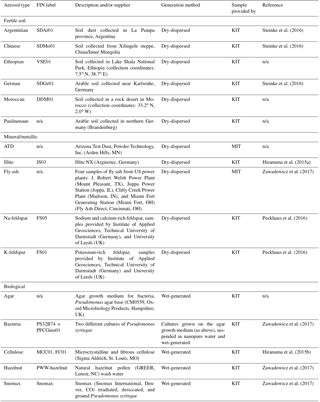
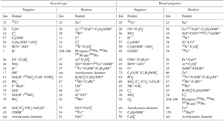
Table 2 Features rankings for differentiation of particles between labels and between broad categories in positive and negative ion modes. See text for additional details. “n/a” stands for not applicable.

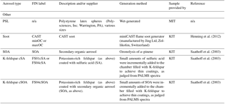
Figure 1 illustrates a simple differentiation of particles using only two mass peaks in one (negative) polarity. Mass peaks represent fractional ion abundance, measured as a total signal (ion current) normalized to allow for spectra-to-spectra comparison (Cziczo et al., 2006). In this example, the normalized areas of negative mass peaks 24 (${\mathrm{C}}_{\mathrm{2}}^{-}$) and 16 (O⁻) are plotted. Distinct aerosol types are differentiated by color with clusters forming in this two-dimensional space. Note that spectra of the same aerosol type form distinct clusters (e.g., Arizona Test Dust, ATD), as do similar aerosol classes (e.g., soil dusts). Co-plotted in Fig. 1 are data from the blind experiment. Distinct clusters of spectra from the blind experiment are noticeable and correlate with known clusters. As described in the next section, machine learning algorithms draw “decision boundaries” that best separate different groups of data points based on a set of rules. Machine learning is not bound by the simplistic two-dimensional space shown in Fig. 1 and instead uses all 512 mass peaks and aerodynamic size.

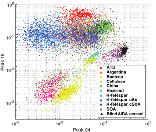
Figure 1 Aerosol training data plotted as feature area 16 (O⁻) versus area 24 (${\mathrm{C}}_{\mathrm{2}}^{-}$). Axes represent peak areas normalized to total signal obtained from PALMS (i.e., 1=100 % of signal). This illustrates simple two-dimensional clustering of aerosols from the training data set by type. Co-plotted are ∼500 randomly drawn spectra from the AIDA blind experiment, which were known to be a subset of the training data aerosols.

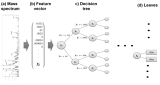
Figure 2 Schematic of decision tree classification for a single aerosol spectrum. From left to right, a mass spectrum is normalized with respect to total ion current, forming the elements of normalized feature vector X. A trained decision tree then applies a series of tests to a discreet number of peaks in order to arrive at a categorical aerosol prediction (the leaves).

2.3 Aerosol classification

A trained classification model maps a continuous input vector X to a discreet output value using a set of parameters “learned” from the data. Figure 2 illustrates the mapping of a mass spectrum to vector space. In contrast to traditional, hard-coded classification methods, machine learning determines parameters that partition the data set. To form X, mass spectra are converted to dimensional vectors normalized to the total ion current (i.e., the total of all mass peaks amounts to 1 in each spectrum). The elements of the vectorized mass spectrum, termed “features”, hold information about the ionization efficiency and relative abundance of chemical species in each aerosol and serve as the variables for the machine learning model.

Machine learning is conducted in two phases: training and testing. During training, a model is constructed and iteratively updated based on data (i.e., mass spectra) from the training set. For this work, the set of known aerosol types sampled by PALMS was converted to dimensional vectors. These data form the basis set for defining each aerosol type. A random forest was used to generate predictions of aerosol type. A single decision tree is a statistical decision model that performs classification based on a series of comparisons relating a variable X_i (in this case a normalized mass peak in X) to a learned threshold value (Breiman, 2001). A random forest is an ensemble of perturbed decision trees, whereby a final classification is made by averaging the predictions across all trees (described below in Sect. 2.4). Represented as an algorithmic tree, a binary decision tree consists of a hierarchy of nodes where each node connects via branches to two other nodes deeper in the tree. At each node, one of the two branches is taken based on whether a normalized peak X_i is greater or less than a threshold value. Each branch leads to another node where a different test is performed. After a series of tests, one at each node, a class is assigned to a given sample; these are the so-called “leaves”. Figure 2 illustrates the classification model for a single decision tree.

Each test in the tree narrows the set of reachable output leaves and thus the sample space of possible aerosol labels. After h tests in this study, where h ranges from 10 to 3000, the set of reachable leaves and possible labels is 1 and the decision tree outputs a prediction. Because PALMS is unipolar – either a positive or negative mass spectrum is produced – simultaneous generation of positive and negative spectra on a particle-by-particle basis is not possible. Two separate classification models, one for each polarity, were generated to classify aerosols. These are hereafter referred to as the “positive” and “negative” classification algorithms.

2.4 Random forests

A random forest is an ensemble of decision tree classifiers where each classifier independently labels an unknown spectrum vector X. To make a final prediction of aerosol type, trees within an ensemble “vote” on a classification label. Each vote has equal weight, and the spectrum is assigned to the majority choice. Each tree within an ensemble is independently grown on a subset of the training data so that a commonly voted-for label implies a higher certainty. Adding members to an ensemble increases the robustness of a classification model by providing alternative hypotheses and is therefore preferable to single classifiers.

Before an ensemble method is implemented for classification, trees are independently grown during training. A total of k trees, with k=110, were grown using a bootstrap sample from the training set. In bootstrap sampling, each tree sees an independent sample set of equal size drawn from the full training set by sampling spectra with replacement. On average, each tree is built with ∼63 % of the original data, leaving a portion of the training set unsampled. The unsampled data for each tree, known as “out-of-bag” observations, are recorded and later provide a means to assess classification error for the forest. To determine model error, predictions are made for each point in the data set using only the subset of trees that did not use the point for training. Each training point is left out at least once. This is analogous to making predictions with a separately trained forest that did not observe the point and prevents testing with the same data used for training.

Given a bootstrap sample, a tree is grown by sequentially creating tests that maximize the separation between classes in parameter space. A test is created by defining a comparison that minimizes the information entropy of a possible split, thus minimizing the randomness of prediction labels (Breiman, 1996). To generate variability in the model, only a random set of splits is tested at each node, and only the best split in terms of entropy is chosen (Breiman, 2001). After iteratively defining thresholds for each new node, the tree grows in size until a series of tests ending at some node S_q uniquely characterizes an aerosol as a particle type. A leaf is then appended to node S_qwith the corresponding label. In classification mode, an aerosol spectrum that passes the same tree will undergo the same series of tests and will end in the same leaf, thus being labeled in the same way. For the purposes of this study, each tree had ∼3300 nodes.

The number of variables per split is chosen to be 11, and the number of trees is 110. Using grid search, the optimal model was determined by enumerating combinations of these parameters on a coarse grid and selecting the values that produce the lowest test error, or out-of-bag error. Given several lists of parameters, where each list corresponds to a different model hyperparameter, models are trained one by one until each combination of parameters has been tested. For this study, the grid representing variables per split was spaced by 1, and the grid for number of trees was spaced by 5. The number of nodes in each tree depends on other hyperparameters and cannot be explicitly set. Model behavior is primarily sensitive to the number of variables per split and shows weak dependence on the number of trees and number of input variables beyond small values. As the number of variable splits increases, error decreases exponentially to a local minimum before again rising due to overfitting. Alternatively, as the number of trees is increased, the error converges to some nonzero value, a known characteristic of random forests where test error converges to the generalization error. The models were trained with the Python 2.7 Scikit-learn module on a MacBook Pro with 16 GB 1600 MHz DDR3 memory and a 2.5 GHz Intel Core i7 processor. A typical random forest model took about 5–10 s to train, and we found a linear relationship between runtime and both the number of trees and variables per split.

Overall, the generalizability and robust performance of random forests is owed significantly to the series of random statistical procedures used to construct such models. An ensemble classifier reduces variability by averaging predictions over a series of independently trained models, and bagging introduces additional randomness by producing “perturbed” versions of the original data via random sampling of input data. The randomness used in constructing forests, both in bagging the training set and choosing variable splits, works to decorrelate the output of each tree even as the inputs become correlated (Breiman, 2001). As the number of trees increases, the law of large numbers guarantees a convergence of the out-of-bag error to the generalization error.

2.5 Dimensionality reduction and chemical feature selection

Dimensionality reduction is the process of representing data with fewer variables than initially present in the data set, in this case less than the original 512 mass peaks and aerodynamic size. In addition to facilitating data visualization, reducing computation time, and limiting overfitting (Mjolsnes, 2001), dimensionality reduction, in the context of aerosol mass spectra, also indicates the most important chemical markers for differentiation. Feature ranking was algorithmically determined by comparing the performance of trees before and after removing information about peak X_i. The method is that the values of variable X_i are permuted for tree k in the out-of-bag set so that the variable is irrelevant to the final label. The change in misclassification before and after the permutation is calculated and then repeated for all trees so that a variable ranking is obtained (Breimann, 2001). Table 2 ranks mass peaks (features) by polarity in importance using this method. The columns on the left list feature rankings (i.e., most to least important for correct classification) for the entire set of aerosol types. The columns on the right list rankings when aerosol types are grouped into the broad, chemically similar, categories. A final ranking was determined by sequentially adding variables and observing classification performance response. All variables preceding two e-foldings in classification error were maintained in the final model. Both the specific aerosol type and broad aerosol category models were retrained using this subset of the initial variables, listed in Table 2.

2.6 Comparison to Euclidean distance classifier

To access relative model performance, we contrast the results with a simple classifier that compares unseen aerosols to a set of class mean vectors. Using the Euclidean distance metric, the unknown aerosol is assigned to the nearest class. This simple baseline classifier helps to put results in the context of machine learning techniques that rely on distance-based metrics such as k-means and hierarchical clustering. K-means clustering attempts to divide the data points into k distinct clusters, representing spectra as vectors. Using Euclidean distance, the standard algorithm assigns points to centroids, or clusters, which are essentially mean vectors representing the average of all points in the cluster. Assuming perfect convergence of k-means clustering, where k is the number of aerosol classes, each cluster represents the mean of aerosol in that class. The random forest results below demonstrate many areas of improvement over the simple classifier.

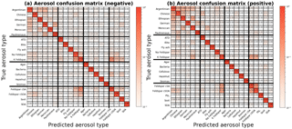
Figure 3 Column-normalized confusion matrices showing fraction of aerosols labeled as j that belong to i, where i and j are row and column indices, respectively. Confusion matrices are determined from training data of known origin and are used to compute probability distributions. Aerosol types (Table 1) are grouped into four broad categories delineated by the bold horizontal and vertical bars. From top to bottom or left to right: fertile soils, mineral/metallic, biological, and other. Classification accuracy, the average probability of a correct aerosol prediction across all labels, is computed by averaging diagonal matrix elements. For all aerosol types, the accuracy is 87 % in positive ion mode and 87 % in negative ion mode.

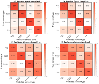
Figure 4 Column-normalized confusion matrices for the broad categorization of aerosols following the convention in Fig. 3. (a, b) For all aerosol categories, the random forest has an accuracy of 93 % in positive ion mode and 91 % in negative ion mode. (c, d) The Euclidean distance classifier has an accuracy of 70 % in positive ion mode and 69 % in negative ion mode.

3 Results

3.1 Confusion matrices and probabilistic model performance

A confusion matrix captures misclassification tendencies by pair-wise matching the model prediction with the true aerosol type or broad category (Powers, 2007) and can be understood as a contingency table matching model predictions to true labels. Confusion matrices represent model predictions as columns i and true aerosol type or category as rows j,where class names are mapped to integers i, $j\in \mathit{\{}\mathrm{1},\mathrm{2},\mathrm{\dots },y\mathit{\}}$. In this study, matrices have been normalized along each column to show the fraction of aerosols labeled as j that actually belong to i (Figs. 3 and 4). For aerosol classification, these matrices can also be interpreted as similarity measures between particle types. Since the basis of classification is separation of physical quantities, misclassifications result from similarity in mass peaks and their ion abundance between aerosol types. This is most easily visualized as overlapping clusters in the simple two-dimensional space in Fig. 1.

Model performance for each aerosol is summarized in the diagonal elements of the confusion matrix P, which represent the fraction of aerosol in column j labeled correctly. The classification accuracy (a) is given by averaging diagonal elements of P. A perfect classification model produces the identity matrix, as all data points are classified correctly 100 % of the time. For example, in the positive confusion matrix, SOA and agar growth medium are correctly labeled in the test set 100 % of the time. Barring element truncation, all columns of P add to 1.

Figures 3 and 4 display confusion matrices as heat maps for the full set of particle labels and broad grouped particle categories, respectively. Broad categories are delineated by bold horizontal and vertical lines in Fig. 3 as fertile soil (Argentinian, Chinese, Ethiopian, Moroccan, and two German soils), pure mineral dust and metallic particles (ATD, illite NX, fly ash, Na-feldspar, and K-feldspar), biological particles (agar growth medium, P. syringae bacteria, cellulose, Snomax, and hazelnut pollen), and other particles (K-feldspar with sulfuric acid (SA) and SOA coatings, soot, and SOA). Some model confusion exists between fertile soils and coated/uncoated feldspars which can be explained by the fact that soils are mineral dust mixed with organic and other materials.

Positive mass spectra appear to hold more information with respect to differentiating aerosols than negative mass spectra. Label-wise classification accuracy for the negative algorithm ranges from 3 to 5 % lower. A large part of this performance discrepancy is due to greater ability of positive spectra to differentiate coated particles within the “other” category.

In addition to quantifying misclassification tendencies between classes, the confusion matrix can be redefined to show confusion for aerosols within broad categories themselves. The precision score (Powers, 2007) captures the classification behavior for some subset of aerosol L by averaging fractions of correctly classified aerosols for labels within that category:

$$\begin{array}{}\text{(1)}& {\displaystyle }\mathrm{precision}\mathrm{score}\left(L\right)={\displaystyle \frac{\mathrm{1}}{\mathrm{|}L\mathrm{|}}}\sum _{i=j}^{\mathrm{|}L\mathrm{|}}P(i\in L,j\in L).\end{array}$$

When applied to P_l, the precision score captures classification performance in a population with only aerosol labels contained in L. The algorithm is expected to correctly label an aerosol in such a population with a probability equal to the precision score. The precision score is valuable when using the classification model as a particle screener, producing probability distributions over a subset of aerosol labels of interest. The confusion characteristics are shown in Table 3 for each category in terms of the precision score and the mean and standard deviation of misclassification within each category. Although both models perform similarly for biological spectra, discrepancies of 2–5 % appear in the remaining categories. For regimes consisting of only mineral/metallic or other particles, the positive algorithm shows intraclass performance advantages not only in terms of the precision score but also, most notably, in terms of fewer mislabeling of mineral/metallic particles. The largest precision discrepancy is observed for fertile soils, where the positive ion algorithm has a 5 % advantage in precision with approximately half the false labeling rate.

Table 3 Model performance by category and ion mode in a population consisting entirely of aerosols within that category. (a) Average classification accuracy where 1.0=100 % precision (Powers, 2007). (b) Mean and standard deviations of misclassification.

Across all categories, the random forest shows improvements over the Euclidean classifier in terms of both accuracy and precision. Figure 4 directly compares confusion matrices for the two methods, revealing overall accuracy improvements of at least 20 %. The largest improvements are in the fertile soil and other category, where accuracy rises between 20 % and 39 % with the random forest. Computing the full confusion matrix for the Euclidean technique (as in Fig. 3) reveals similar results, with far more frequent mislabeling between fertile soils and coated/uncoated particles than our approach. These results reinforce the fact that chemically similar aerosols which overlap in feature space will often be grouped together when using a single distance-based classifier. The improvement from random forests is likely a result of (a) the ensemble approach, which is known to produce better generalizability than single classifiers, and (b) the tendency of aerosols with similar chemical properties and atmospheric effect to appear mathematically distinct with a distance metric.

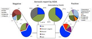
Figure 5 Model predictions of ∼5000 aerosols sampled from the AIDA FIN01 blind mixture, which was known to be a subset of the training data. All percentages represent relative number concentrations. Middle left: aerosol types input to the chamber for the blind mixture. Middle right: aerosol types input to the chamber for the blind mixture and above the detection limit for PALMS. Model predictions are shown for negative and positive ion mode on the left and right, respectively. Bottom: broad categories. Top: breakout by aerosol type of the non-SOA categories above the 1 % level. Note that (1) the soot in the blind mixture was known to be below the instrument detection limit and therefore is not expected to be found in the data (Cziczo et al., 2006); (2) coagulation of SOA and mineral dust, which occurred after aerosol input to the chamber, was often categorized as mixed mineral and organic particles or fertile soils (i.e., mixtures of mineral and organic components) considered in the training data set; and (3) the aerosols types reported by AIDA do not account for PALMS transmission efficiency (see text for details).

Beyond classification, the obtained variable rankings alone provide interesting insights into the data set. It is noteworthy that while most of the features are logical differentiators of the aerosol types investigated in FIN01 there were also surprises. One example is 59⁺ (cobalt), determined to be one of the most important features for differentiation. Further investigation determined this material was associated with tungsten carbide contaminant from dry-powder-dispersion equipment used on some samples. The contamination affected feldspar samples used during the second half of the AIDA measurements in particular. This serves to illustrate the lack of a priori judgment by the algorithm and an unintended benefit of machine learning processes (i.e., contamination identification).

3.2 Characterization of blind data

As part of the FIN01 workshop, an a priori unknown number of aerosol types from Table 1 were aerosolized into the AIDA chamber at unknown size and relative concentration. PALMS, one member of the blind intercomparison effort, collected ∼25 000 spectra. After data analysis, the aerosol types and relative abundances were provided to each group (Fig. 5, top center).

The presence or absence of particle types in the blind set was initially diagnosed by choosing particles predicted at or above the 1 % level. We note here that this step was based on the knowledge that (1) a distinct set of particles would be placed in the chamber and (2) particles present at or below the 1 % level were most likely contaminated. We further note that this step is unique to a blind study and would not be applicable to the atmosphere.

Figure 5 illustrates the fractional percentages for each aerosol category. Because SOA was nearly always labeled correctly (Fig. 3), the remaining aerosols are considered separately using the full set of candidate aerosol labels. Both positive and negative models arrived at similar results, with inconsistencies primarily associated with the presence of trace fertile soils and mineral dust/fly ash particles. The positive algorithm identifies Argentinean soil, German soil, ATD, and cellulose as each comprising ∼2–4 % of the AIDA population, whereas the frequency of these aerosols was too low to consider in the negative algorithm. Alternatively, the negative model estimates Na-feldspar at ∼14 % of the total population, a label not identified by the positive algorithm. This discrepancy can partially be explained by the 1 % selection criterion for aerosols present in the population. Fertile soils, ATD, and cellulose frequently accumulate error along rows in the full positive confusion matrix, indicating frequent confusion with other categories (Fig. 3). Furthermore, with the observed misclassification rates ranging ∼1–4 %, it is expected that these aerosol labels are false positives. The negative model offers an alternative hypothesis, suggesting these miscellaneous aerosols are Na-feldspar. Since there is significant model agreement on the percentages of SOA and coated feldspars, this part of the blind mixture population can be characterized with more certainty. For the disputed aerosol labels, more credence is lent to the negative classification algorithm on the basis of improved precision for fertile soils.

The aerosols reported in the blind mixture were soot, mineral dust, and SOA. The soot aerosols used in the blind study were smaller than in the training data experiments and were below the cutoff diameter for PALMS; they were therefore not detected and therefore could not be identified by the algorithms. This bias in transmission efficiency should be noted, whereby aerosols are detected at a rate that depends on their size and aerodynamic properties (Cziczo et al., 2006). The result is that particles with diameters below ∼200 nm or greater than ∼1000 nm are detected with increasing inefficiency, which leads to relative undercounting of small soot or large mineral dust (Cziczo et al., 2006). The specific mineral component was not identified and may have been either a pure mineral or soil dust. Both algorithms robustly labeled SOA with large agreement, consistent with the 100 % accuracy observed in the test set.

SOA-coated mineral dust was identified as a particle type. This material was not directly input to AIDA, but the report is most likely correct, due to coagulation within the AIDA chamber during the course of the blind experiment. Since percentages were reported before particles entered the chamber, it is not possible to directly verify the fraction of SOA-coated aerosols or the extent to which coagulation occurs, as the process is time dependent. This may also explain some indications of fertile soils, which are known to be mixtures of mineral and organic components. The training data set did not contain coagulated SOA and mineral dust but did include SOA-coated K-feldspar, which explains the identification.

While both models identified a variety of fertile soils, and not a single type, these results are largely consistent with the presence of coagulated organics and minerals and the known uncertainties highlighted by the confusion matrices discussed previously. Given the presence of any single mineral dust, some confusion with fertile soils, SA-coated Feldspar, and Na-feldspar is expected (Fig. 3). Moreover, as discussed previously (Gallavardin et al., 2008a, b), AIDA backgrounds are not completely particle free. During the FIN01 study, contaminated particles from previous test aerosol were frequently observed as background, and they could also be the origin of some low-concentration particles matching fertile soil chemistry. Overall, discrepancies between the reported aerosol fractions and model predictions can be accounted for with model and experiential uncertainties.

An additional consideration is experimental bias in the training data, which could result in test errors that underestimate true generalization errors in real aerosol populations. For SPMS, spurious relationships between spectra may arise due to instrumental parameters that are assumed to be constant between the training, test, and blind data. This consideration plagues all SPMS analysis requiring a training set, where correlations may arise as a result of signals that depend on ambient properties like temperature, humidity, and pressure or instrument parameters such as laser power. Although several well-established steps were taken to minimize overfitting – including dimensionality reduction and out-of-bag testing – data set bias may still exist if these quantities vary significantly between aerosol types in the training or blind data.

4 Conclusions and future work

This study lays out a framework for training and implementing random forests on SPMS data, with a focus on dimensionality reduction and the evaluation of model performance with confusion matrices. A key benefit to the proposed method is chemical feature selection, which allows researchers to identify potentially important chemical markers between arbitrary groups of aerosols or identify sources of contamination. In this particular study, the contaminant was identified and removed in the dimensionality reduction step while reasoning through the subset of ranked features. As illustrated by Fig. 2, cobalt is suspiciously identified as the second-most-important variable for classification, but it is a known component of the dry-powder-dispersion equipment used on some samples. The contaminate peak would be present in a cluster analysis, but it would not be obvious to pick out and remove as standard clustering is not typically suited for variable rankings.

For future studies tackling ambient atmospheric data that may contain aerosol types absent from the training set, a form of subspace selection may be used to improve results. The region of parameter space where training data are available can be characterized with a joint probability density function. One such approach is kernel density estimation – a machine learning method that approximates a multidimensional probability density function in a non-parametric manner based on data density. To obtain accurate probability estimates, the method should be fit with a smaller set of important but uncorrelated peaks. The task of classification is then preceded by a filtering step. Spectra residing in the subspace containing the training data should first be identified based on the probability density function. Then, only these particles that are most certain to lie in the training subspace are classified using the classification model as described in this paper. An alternative is to combine the method with clustering by classifying particles in each automatically identified cluster.

Overall, the random forest approach allows for differentiation of aerosols within a SPMS data set, augmenting existing tools and reducing the need for a qualitative comparison between mass spectra. Across a representative sample of possible aerosol types, the behavior of each algorithm predictably allows users to infer the presence or absence of specific aerosols and quantify aerosol abundance. Machine learning is automated, and the output of the model must then be informed by human knowledge of aerosol chemistry. Machine learning should therefore be considered as an additional tool to interpret mass spectra to better distinguish aerosols with unique properties in terms of atmospheric chemistry, biogenic cycles, and population health.

The random forest classification framework described here may be generalized to any instrument, or set of instruments, capable of collecting physical and chemical information that distinguishes particles. Although the method described here is applied to a stand-alone SPMS and tested with a set of “blind” data, ancillary laboratory or field data can be integrated to expand the data set. The success of these algorithms is data dependent, where better performance is expected for instruments that provide more, and more quantitative, analysis of the aerosol properties. Although the algorithms implemented in this study were primarily used to categorize SOA, mineral dust, fertile soil, and biological aerosols, these models can adopt an arbitrarily large set of aerosol data.