MODIS Collection 6 MAIAC algorithm

This paper describes the latest version of the algorithm MAIAC used for processing the MODIS Collection 6 data record. Since initial publication in 2011–2012, MAIAC has changed considerably to adapt to global processing and improve cloud/snow detection, aerosol retrievals and atmospheric correction of MODIS data. The main changes include (1) transition from a 25 to 1 km scale for retrieval of the spectral regression coefficient (SRC) which helped to remove occasional blockiness at 25 km scale in the aerosol optical depth (AOD) and in the surface reflectance, (2) continuous improvements of cloud detection, (3) introduction of smoke and dust tests to discriminate absorbing fine- and coarse-mode aerosols, (4) adding over-water processing, (5) general optimization of the LUT-based radiative transfer for the global processing, and others. MAIAC provides an interdisciplinary suite of atmospheric and land products, including cloud mask (CM), column water vapor (CWV), AOD at 0.47 and 0.55 µm, aerosol type (background, smoke or dust) and fine-mode fraction over water; spectral bidirectional reflectance factors (BRF), parameters of Ross-thick Li-sparse (RTLS) bidirectional reflectance distribution function (BRDF) model and instantaneous albedo. For snow-covered surfaces, we provide subpixel snow fraction and snow grain size. All products come in standard HDF4 format at 1 km resolution, except for BRF, which is also provided at 500 m resolution on a sinusoidal grid adopted by the MODIS Land team. All products are provided on per-observation basis in daily files except for the BRDF/Albedo product, which is reported every 8 days. Because MAIAC uses a time series approach, BRDF/Albedo is naturally gap-filled over land where missing values are filled-in with results from the previous retrieval. While the BRDF model is reported for MODIS Land bands 1–7 and ocean band 8, BRF is reported for both land and ocean bands 1–12. This paper focuses on MAIAC cloud detection, aerosol retrievals and atmospheric correction and describes MCD19 data products and quality assurance (QA) flags.

1 Introduction

Simple and fast swath-based processing with a Lambertian surface model is the basis of the Moderate Resolution Imaging Spectroradiometer (MODIS) Dark Target (DT) (Levy et al., 2013) and VIIRS (Visible Infrared Imaging Radiometer Suite; Jackson et al., 2013) aerosol retrievals and atmospheric correction (AC) (Vermote and Kotchenova, 2008). In swath data, the satellite footprint and its location are orbit dependent and change with scan angle, making it difficult to characterize the surface BRDF. The above algorithms rely on prescribed spectral surface reflectance (SR) ratios to make aerosol retrievals. The SR ratios represent statistically average relationships with relatively large variance. When the surface brightness increases and sensitivity of the top of atmosphere (TOA) radiance to aerosols decreases, this lack of accurate knowledge of surface reflectance becomes a major issue.

The Multi-Angle Implementation of Atmospheric Correction (MAIAC) algorithm uses a physical atmosphere–surface model where the model parameters are defined from measurements (Lyapustin et al., 2011a, b, 2012a, b) with minimal assumptions. Instead of swath-based processing, we start with gridding MODIS L1B measurements to a fixed 1 km grid and with accumulating a time series of data for up to 16 days using a sliding window technique. This allows us to observe the same grid cell over time, helping to separate atmospheric and surface contributions with the time series analysis and characterize surface bidirectional reflectance distribution function (BRDF) using multi-angle observations from different orbits. Besides BRDF retrieval, the fixed surface representation (grid) allows us to characterize and store unique surface spectral, spatial, thermal, etc. signatures for each 1 km grid cell, helping to increase the accuracy of the entire processing, from cloud and snow detection to aerosol retrievals and atmospheric correction (AC).

Since its introduction in 2011–2012, we have significantly changed and improved several key parts of MAIAC, namely cloud and snow detection, characterization of the spectral regression coefficient (SRC) and aerosol retrieval, and transformed the algorithm from regional to global. The intermediate versions of MAIAC were continuously tested by the land and air quality communities using our processing of MODIS data with the NASA Center for Climate Simulations (NCCS) and product release via NCCS ftp portal (ftp://maiac@dataportal.nccs.nasa.gov/DataRelease, last access 9 October 2018). Analysis by Hilker et al. (2012, 2014, 2015), Maeda et al. (2016) and others showed a dramatic (up to a factor of 3–5) increase in the accuracy of MAIAC surface reflectance compared to MODIS standard products MOD09, MOD035 over the tropical Amazon. Since 2014, all major studies of Amazon tropical forests, which used MODIS data, relied on MAIAC processing (e.g., Saleska et al., 2016; Lopes et al., 2016; Alden et al., 2016; Guan et al., 2015; Bi et al., 2015, 2016; Jones et al., 2014; Maeda et al., 2017; Wagner et al., 2017). Recently, Chen et al. (2017) reported an improvement in the leaf area index (LAI) retrievals with the MODIS LAI/FPAR algorithm when using MAIAC instead of standard MODIS MOD09 input. A high accuracy, high 1 km spatial resolution and high retrieval coverage made MAIAC aerosol optical depth (AOD) a focus of numerous air quality studies, e.g., Chudnovsky et al. (2013), Kloog et al. (2014), Just et al. (2015), Di et al. (2016), Stafoggia et al. (2016), Tang et al. (2017) and Xiao et al. (2017) to name a few. Currently published validation studies (Martins et al., 2017; Superczynski et al., 2017) show a high MAIAC AOD accuracy over American continents and an improved accuracy and coverage over North America compared to the operational VIIRS algorithm (Superczynski et al., 2017). An emerging comparative aerosol validation analysis over North America (Jethva et al., 2018) and southern Asia (Mhawish et al., 2018) shows that MAIAC has a comparable or better accuracy than the DT algorithm over dark surfaces and generally improves accuracy over the Deep Blue (DB) algorithm (Hsu et al., 2013) over bright surfaces.

The MAIAC MODIS Collection 6 (with enhanced calibration (C6+), which added polarization correction of MODIS Terra, removed residual trends of both Terra and Aqua, and cross-calibrated Terra to Aqua (Lyapustin et al., 2014b) processing is ongoing on the MODIS Adaptive Processing System (MODAPS). It is expected to be completed in the spring of 2018, creating a new MODIS product MCD19 accessible via the Land Product Distributed Active Archive Center (LP DAAC). MAIAC offers an interdisciplinary suite of products for the Land, Atmosphere, Cryosphere and Applications communities including cloud/snow mask over land, high spatial resolution (1 km), aerosol optical depth and type, surface bidirectional reflectance factors (BRF) and BRDF, and snow grain size and subpixel snow fraction for the snow-covered regions.

The goal of this paper is to give a systematic description of the MAIAC Collection 6 algorithm and its products, along with current limitations, and provide quality assurance discussion and recommendations for use. For practical reasons, here we focus on MAIAC cloud detection, aerosol retrieval and atmospheric correction over land; snow detection, over-water processing and smoke plume height retrieval will be described elsewhere. This paper is structured as follows: an overview of MAIAC processing is given in Sect. 2; Sect. 3 describes the MAIAC radiative transfer model and lookup tables followed by MAIAC processing components, including cloud/snow detection and aerosol-type selection (Sect. 4), determination of SRC (Sect. 5) and aerosol retrieval procedures (Sects. 6–7), shadow detection (Sect. 8) and atmospheric correction (Sect. 9). Sect. 10 describes the MAIAC (MCD19) product and its quality assurance (QA) specification.

2 Overview of MAIAC processing

The block diagram of MAIAC processing over land, which implements a sliding window algorithm, is shown in Fig. 1:

Figure 1 Block diagram of MAIAC algorithm.

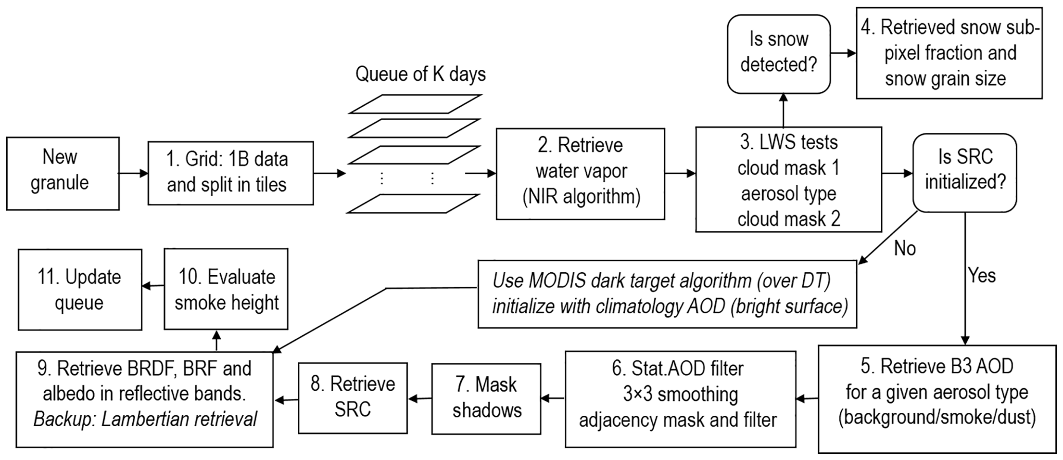
• 1.

  The received L1B data are gridded (Wolfe et al., 1998), split into 1200 km tiles and placed in a queue with the previous data. We are using the area-weighted gridding method, which achieves better agreement with the ground tower data over heterogeneous surfaces compared to the nearest-neighbor resampling method (Zhang et al., 2014). The 1 km MODIS bands are gridded to 1 km resolution, the 500 m bands (B1–B7) are gridded to 1 km and 500 m and 250 m bands (B1–B2) are gridded to 250 m. The 500 and 250 m bands are nested in the 1 km grid. For convenience, here is the list of MODIS bands B1–B12, where MAIAC reports BRF at 1 km: 0.645 (B1), 0.856 (B2), 0.465 (B3), 0.554 (B4), 1.242 (B5), 1.629 (B6), 2.113 (B7), 0.412 (B8), 0.442 (B9), 0.487 (B10), 0.530 (B11), 0.547 (B12).

  MAIAC uses different spatial scales for processing, e.g., 1 km grid cells (or pixels), 25 km blocks and 150 km mesoscale areas. Specialized C$++$ classes and structures handle processing in different time–space scales. The queue (Q) (Lyapustin et al., 2012a) holds between 4 (at the poles) and 16 (at the equator) days of imagery. For every observation, MODIS data are stored as layers for the required bands along with the retrieval results. A dedicated Q memory accumulates ancillary information for each 1 km grid cell for cloud/snow detection, aerosol retrieval and AC. Q memory stores the following data at 1 km resolution: the reference clear-sky image for bands B1, B3, B7 (see Lyapustin et al., 2008); spectral BRDF for bands B1–B8; BRDF-normalized (to nadir view and solar zenith angle, SZA = 45 ^∘) bidirectional reflectance factors BRF_n for bands B1, B2, B7; 2×2standard deviation of 500 m pixels for B1, B3; normalized difference vegetation index (NDVI); 11 µm brightness temperature (Tb₁₁, band 31); 4 µm (B22)–11 µm (B31) (Tb${}_{\mathrm{4}-\mathrm{11}}={\mathrm{Tb}}_{\mathrm{4}}-{\mathrm{Tb}}_{\mathrm{11}}$) and 11–12 µm (B32) (Tb${}_{\mathrm{11}-\mathrm{12}}={\mathrm{Tb}}_{\mathrm{11}}-{\mathrm{Tb}}_{\mathrm{12}}$) spectral thermal contrasts. Below, we will use notation q.Tb₁₁ for the queue brightness temperature as an example.

  Prior to processing, we compute the covariance of the latest measurements with the reference clear-sky image (Lyapustin et al., 2008) in bands B3, B1 and B5 for 25×25 km² blocks. When covariance is high, indicating high probability for the confidently clear conditions, we later set the corresponding flag q.iFlag_HighCov =1 used in the cloud detection (see test C4, Sect. 4.1).

• 2.

  The column water vapor is computed for the last tile using MODIS near-IR channels B17–B19 located in the water vapor absorption band 0.94 µm (Lyapustin et al., 2014a). This algorithm is a modified version of Gao and Kaufman (2003). It is fast, unbiased and has an average accuracy of ±(5–15) % over the land surface (ATBD; Martins et al., 2017), whereas the standard NIR CWV product (MOD05) has a known wet bias of 5 %–20 % (e.g., Albert et al., 2005; Prasad and Singh, 2009; Liu et al., 2013).

  Column water vapor is retrieved over cloud-free land pixels and over clouds. In the latter case, it represents water vapor above the cloud.

• 3.

  The cloud mask box includes dynamic land–water–snow classification, determination of aerosol type (background vs. smoke or dust) and cloud detection. The smoke/dust test is based on the enhanced shortwave absorption and effective particle size (Lyapustin et al., 2012c) and requires knowledge of spectral surface BRDF. At 1 km resolution, brightness and spatial contrasts of smoke plumes can be high, leading to competition between smoke and cloud detection. With optimal combination of different cloud tests and smoke detection, which was found experimentally based on large-scale MODIS data processing, MAIAC provides aerosol retrievals for most smoke plumes with minimal cloud leak.

• 4.

  When snow is detected, MAIAC derives surface reflectance using regional climatology AOD and computes snow grain size (SGS) and subpixel snow fraction (SF) as best fit to obtained spectral reflectance. The reflectance is modeled as a linear mixture of snow BRDF and land BRDF, which is stored in the queue from retrievals prior to snow detection. Snow reflectance is modeled with a semi-analytical model (Kokhanovsky and Zege, 2004), with consideration for surface roughness (Lyapustin et al., 2010). Assuming a background soot concentration, the snow reflectance depends only on SGS, which is computed from measured spectrum along with SF. The algorithm is analytical, fast and robust due to a large difference between spectra of regular land types and snow. The derived SGS may have a large uncertainty because of rapid metamorphism of aging snow and pollution from the atmosphere, which reduce snow reflectance. We validated SGS retrievals over pure snow (Lyapustin et al., 2009). The algorithm description and validation of snow fraction using high-resolution Landsat data will be given elsewhere.

• 5-6.

  Using knowledge of spectral BRDF and SRC at 1 km, MAIAC retrieves AOD at 1 km resolution. The following post-processing uses several filters to detect residual clouds and smooth the noise from gridding uncertainties. This step significantly increases the quality of AOD and the atmospheric correction.

• 7.

  The combination of MAIAC cloud mask and AOD filters (6) detects majority of clouds. The next step (7) detects cloud shadows using a geometric approach and our knowledge of BRDF.

• 8.

  The spectral regression coefficient (SRC) required for aerosol retrieval is determined.

• 9.

  In cloud-free and clean-to-moderately-hazy (AOD_0.47<1.5) conditions, MAIAC atmospheric correction computes spectral BRF at 1 km resolution (bands B1–B12) and at 500 m resolution (bands B1–B7). By combining BRF from the latest observation with previous values stored in the queue, MAIAC performs a BRDF inversion in 1 km bands 1–8, providing three parameters of the Ross-thick Li-sparse (RTLS) BRDF model (Lucht et al., 2000).

• 10.

  Aerosol layer height for detected smoke pixels is evaluated using a thermal technique (Lyapustin et al., 2018d).

• 11.

  At the end of the processing, the Q memory is updated for cloud-free pixels under clean atmospheric conditions.

As ancillary data, MAIAC uses static DEM, a 1 km land–water mask for deep and static water, and 6 h NCEP ozone and wind speed.

3 Radiative transfer model and lookup tables

MAIAC radiative transfer (RT) model uses a semi-empirical Ross-thick Li-sparse (RTLS) BRDF model (Lucht et al., 2000) used in the operational MODIS BRDF/Albedo (MOD35) algorithm (Schaaf et al., 2002). This is a linear model, represented as a sum of Lambertian, geometric-optical and volume scattering components:

$$\begin{array}{}\text{(1)}& \mathit{\rho }({\mathit{\mu }}_{\mathrm{0}},\mathit{\mu },\mathit{\varphi })=k^L+k^G{f}_{\mathrm{G}}({\mathit{\mu }}_{\mathrm{0}},\mathit{\mu },\mathit{\varphi })+k^V{f}_{\mathrm{V}}({\mathit{\mu }}_{\mathrm{0}},\mathit{\mu },\mathit{\varphi }).\end{array}$$

It uses predefined geometric functions (kernels), f_G and f_V, to describe different shapes as a function of view geometry (μ₀, μ, ϕ – cosines of solar and view zenith angles, and relative azimuth). The kernels are independent of the land conditions. The BRDF of a pixel is characterized by a combination of three kernel weights, $\mathit{K}=\mathit{\{}{k}^L,k^G,k^V{\mathit{\}}}^{\mathrm{T}}$.

MAIAC RT model is based on the semi-analytical Green's function (GF) solution for the TOA reflectance (Lyapustin and Knyazikhin, 2001). When combined with the linear RTLS model, the GF solution provides an explicit expression for the TOA reflectance as a function of the RTLS model parameters (Lyapustin et al., 2011a):

$$\begin{array}{ll}{\displaystyle }R({\mathit{\mu }}_{\mathrm{0}},& {\displaystyle }\mathit{\mu },\mathit{\varphi })=R^{\mathrm{A}}({\mathit{\mu }}_{\mathrm{0}},\mathit{\mu },\mathit{\varphi })+k^L{F}^L({\mathit{\mu }}_{\mathrm{0}},\mathit{\mu })\\ {\displaystyle }& {\displaystyle }+k^G{F}^G({\mathit{\mu }}_{\mathrm{0}},\mathit{\mu },\mathit{\varphi })+k^V{F}^V({\mathit{\mu }}_{\mathrm{0}},\mathit{\mu },\mathit{\varphi })\\ \text{(2)}& {\displaystyle }& {\displaystyle }+R^{\mathrm{nl}}({\mathit{\mu }}_{\mathrm{0}},\mathit{\mu }).\end{array}$$

Here, R^A is atmospheric path reflectance. Functions $F^L,F^V,F^G,R^{\mathrm{nl}}$ depend on view geometry and aerosol properties. They are also weakly nonlinear functions of K parameters, which account for multiple reflections of sunlight between the land surface and the atmosphere. This dependence is analytical and is conveniently handled by the second iteration during the atmospheric correction. The details for computing functions F^j, R^nl are given by Eqs. (1)–(25) in Lyapustin et al. (2011a). In brief, they are expressed via eight basic functions which represent different hemispheric integrals from downward path radiance, atmospheric Green's function (or bidirectional upward diffuse transmittance) and RTLS kernels (1, f_V, f_G). These functions, along with path reflectance, are precomputed and stored in the lookup table (LUT). Throughout this paper, AOD refers to the blue wavelength (AOD_0.47).

Equation (2) is used in MAIAC cloud detection, selection of aerosol type and in the atmospheric correction. For SRC and aerosol retrieval, we also use Lambertian equivalent reflector (LER) approximation,

$$\begin{array}{ll}{\displaystyle }R({\mathit{\mu }}_{\mathrm{0}},& {\displaystyle }\mathit{\mu },\mathit{\varphi })\cong R^{\mathrm{A}}({\mathit{\mu }}_{\mathrm{0}},\mathit{\mu },\mathit{\varphi })+\mathit{\rho }({\mathit{\mu }}_{\mathrm{0}},\mathit{\mu },\mathit{\varphi }\left)T^{\mathrm{d}}\right({\mathit{\mu }}_{\mathrm{0}}\left)T^{\mathrm{u}}\right(\mathit{\mu })\\ \text{(3)}& {\displaystyle }& {\displaystyle }/\left(\mathrm{1}-s\mathit{\rho }({\mathit{\mu }}_{\mathrm{0}},\mathit{\mu },\mathit{\varphi })\right),\end{array}$$

where T is the total downward (d) and upward (u) transmittance, and s is spherical albedo of atmosphere. Over the water, Eq. (3) is modified to account for the diffuse reflectance ρ^w of underlight, representing water-leaving radiance:

$$\begin{array}{ll}{\displaystyle }R({\mathit{\mu }}_{\mathrm{0}},& {\displaystyle }\mathit{\mu },\mathit{\varphi })\cong R^{\mathrm{A}+\mathrm{s}}({\mathit{\mu }}_{\mathrm{0}},\mathit{\mu },\mathit{\varphi })+{\mathit{\rho }}^{\mathrm{w}}({\mathit{\mu }}_{\mathrm{0}},\mathit{\mu },\mathit{\varphi })\\ \text{(4)}& {\displaystyle }& {\displaystyle }{T}^{\mathrm{d}}\left({\mathit{\mu }}_{\mathrm{0}}\right)T^{\mathrm{u}}\left(\mathit{\mu }\right),\end{array}$$

where R^A+s contains Fresnel reflectance from wind-ruffled ocean surface and a whitecap contribution (Koepke, 1984) in addition to the atmospheric path reflectance.

Since Lyapustin et al. (2011a), MAIAC aerosol models and LUTs were simplified considerably. We abandoned approach of mixing fine- and coarse-aerosol fractions in favor of using regional aerosol models based on AERONET climatology (Holben et al., 1998) (e.g., Dubovik et al., 2002; Eck et al., 2013). C6 MAIAC uses eight regional aerosol models and the respective LUTs (see Sect. 6) over land, including a separate dust model. Since MAIAC processing is tile-based and inherently regional, it only reads the required regional LUT or LUTs without overloading operational memory. This allows us to discretize the world map in sufficient detail to account for the regional aerosol variability.

Each LUT is computed with full multiple scattering: all functions are first computed using LUT-generation software based on scalar code SHARM (Lyapustin, 2005), and the atmospheric path reflectance is then replaced with vector solution from code IPOL. The discrete ordinates code IPOL was recognized as the best overall among 10 different vector codes which participated in the recent intercomparison study (Emde et al., 2015).

Each LUT is generated for the standard P=1 and reduced (P=0.7) pressure levels (normalized to the standard pressure 1013.25 mB) in order to account for surface height variations using linear interpolation. Because Rayleigh optical depth rapidly decreases with wavelength, computations with P=0.7 are done for wavelengths shorter than 0.66 µm.

As before, the spectral gaseous absorption used in the LUT radiative transfer was obtained based on the line-by-line calculations (Lyapustin, 2003) for MODIS spectral response functions. The computations include absorption of six major atmospheric gases (H₂O, CO₂, CH₄, NO₂, CO, N₂O) calculated for the HITRAN 2008 (Rothman et al., 2009) database using the Voigt vertical profile and the Atmospheric Environmental Research (AER) continuum absorption model (Clough et al., 2005). The LUT is generated for a fixed value of column water vapor, W₀=0.5 cm. In the MODIS red band, where WV absorption is maximal, the atmospheric path reflectance is also generated for WV = 6 cm, and linear interpolation is used to account for the WV variations.

For the pressure and WV correction, the surface-reflected signal is multiplied by the two-way direct transmittance of the well-mixed gases and water vapor t^g(P)t(W₀,W):

$$\begin{array}{ll}\text{(5)}& {\displaystyle }& {\displaystyle }{t}^{\mathrm{g}}\left(P\right)=\exp \left(-(\mathrm{1}-P){\mathit{\tau }}^{\mathrm{g}}m\right),m={\left|\mathit{\mu }\right|}^{-\mathrm{1}}+{\mathit{\mu }}_{\mathrm{0}}^{-\mathrm{1}},{\displaystyle }& {\displaystyle }t(\mathit{\lambda },W)=\exp \left(-a(\mathit{\lambda },W)m^{b(\mathit{\lambda },W)}\right),t\left(W_{\mathrm{0}},W\right)\\ \text{(6)}& {\displaystyle }& {\displaystyle }=t(\mathit{\lambda },W)/t(\mathit{\lambda },W_{\mathrm{0}}).\end{array}$$

Above, m is an atmospheric air mass, and parameters a and b are obtained by fitting the angular dependence of the water vapor in-band transmittance. Expression (5) is a modified form of equation for the broadband transmittance of water vapor (Schmid et al., 2001).

Finally, LUTs are computed for a relatively sparse angular grid ($\mathrm{\Delta }{\mathit{\mu }}_{\mathrm{0}}=\mathrm{\Delta }\mathit{\mu }=\mathrm{0.05}$ for the range μ=0.4–1 (0–66.42^∘), μ₀=0.15–1 (0–81.37^∘) and Δϕ=9^∘) and 12 AOD values, $\mathit{\{}\mathrm{0.05},\mathrm{0.1},\mathrm{0.2},\mathrm{0.3},\mathrm{0.4},\mathrm{0.55},\mathrm{0.75},\mathrm{1}.,\mathrm{1.4},\mathrm{2.0},\mathrm{2.8},\mathrm{4.0}\mathit{\}}$, giving the size of 45.7 MB per regional aerosol model. Rayleigh LUT (AOD = 0) is generated separately.

Ordinarily, generating LUT-based TOA reflectance for shortwave channels requires two 3-D interpolations in angles at P=1, 0.7, with the following linear interpolation in pressure for a number of required functions per pixel. To optimize MAIAC processing, we introduced intermediate-scale radiative transfer RT containers for 5 km boxes. Each box is characterized by an average view geometry, mean water vapor and surface pressure, representing the average height. For each box, we compute the required functions for 13 AOD LUT nodes. After that, specific MAIAC processing for any 1 km pixel within a given 5 km box only requires an additional linear interpolation in AOD using functions from the RT container and an analytical WV correction for the surface-reflected signal. The 5 km RT containers (RT₅) are generated for boxes with cloud-free pixels and are stored as a layer in the queue. This approach allows us to use the same RT container repeatedly at different stages of MAIAC processing, which reduces computational cost by at least a factor of 25. While theoretically such approach may create biases at short wavelengths (B3 (0.47 µm) and B8 (0.412 µm)) on the boundaries of boxes with a sharp height gradient, a very extensive near-global testing did not reveal any noticeable difference in AOD or surface BRF compared to the accurate 1 km pixel-level interpolation in view geometry and pressure.

Prior to processing of a new MODIS observation, we compute a spectral deviation of measurements (M) from the expected theoretical (T) clear-sky (AOD = 0) TOA reflectance:

$$\begin{array}{}\text{(7)}& {\mathit{\delta }}_{\mathit{\lambda }}=R_{\mathit{\lambda }}^{\mathrm{M}}-R_{\mathit{\lambda }}^{\mathrm{T}}({\mathit{\tau }}^a=\mathrm{0}).\end{array}$$

δ_λ is computed for five bands (B1, B3, B8, B5, B7) and is indicative of atmospheric perturbations from clouds and aerosols as illustrated in Fig. 2 for band B3. Because MAIAC freezes BRDF retrievals when snow is detected such that the queue BRDF always represents snow-free land reflectance, δ_λ also contains spectral signatures of snow and is used in snow detection.

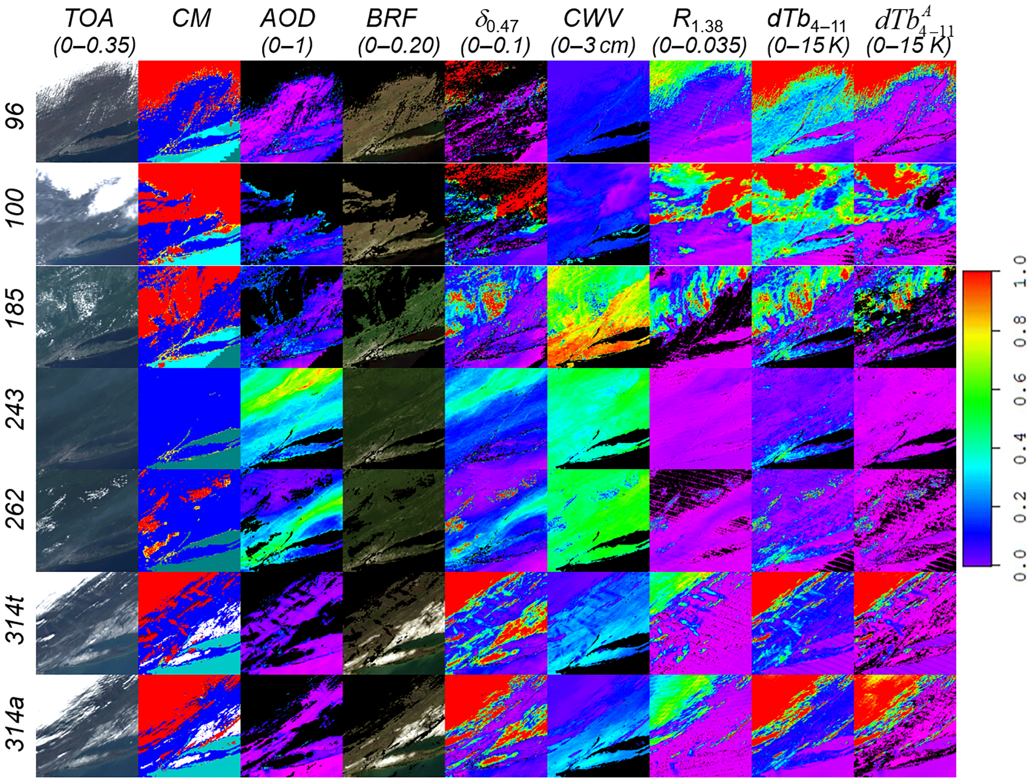
Figure 2 Illustration of MAIAC time series processing for the mid-Atlantic USA 250 km region with New York City in the lower-left corner. The rows show MODIS observations for different days of the year (DOY) for 2012. The two bottom rows show DOY 314 from Terra and Aqua. The columns present the MODIS TOA RGB image, MAIAC products (cloud mask, AOD_0.47, RGB BRF, column water vapor) and some of the internal fields used in the processing (deviation from clear-sky δ_0.47, cirrus band reflectance R_1.38, thermal contrast, dTb₄₋₁₁ and its atmospheric part, dTb${}_{\mathrm{4}-\mathrm{11}}^{\mathrm{A}}$). Columns 3, 5–9 are displayed using the rainbow palette with the (min–max) values shown in the heading in parentheses. The cloud mask uses the following legend: cloud (red), possibly cloudy (yellow), cloud shadow (dark red), clear land (blue), clear snow (white), clear water (light blue), clear water, detected sediments (grey), glint over water (dark grey).

Using an estimate of Jacobian in the blue band (B3), $\partial R/\partial {\mathit{\tau }}^a\approx \left(R^{\mathrm{T}}\right(\mathrm{0.05})-R^{\mathrm{T}}(\mathrm{0}\left)\right)/\mathrm{0.05}$, it is easy to obtain an initial assessment of AOD,

$$\begin{array}{}\text{(8)}& {\mathit{\tau }}_{\mathrm{0}}^a={\mathit{\delta }}_{\mathrm{0.47}}(\partial R/\partial {\mathit{\tau }}^a{)}^{-\mathrm{1}},\end{array}$$

which appears quite accurate except over bright surfaces. To guide aerosol retrievals, we also evaluate a theoretical uncertainty of AOD in response to uncertainty in the surface reflectance at 0.47 µm which is assumed as $\mathit{\delta }\mathit{\rho }=\max \mathit{\{}\mathrm{0.002};\mathrm{0.04}\mathrm{RTLS}({\mathit{\mu }}_{\mathrm{0}},\mathit{\mu },\mathit{\varphi }\left)\mathit{\right\}}$. This estimate is based on the extensive evaluation of MAIAC retrieval accuracy, although it may overestimate the uncertainty over bright surfaces. Given δρ and neglecting other contributions, e.g., from variation in the aerosol model, the AOD uncertainty is as follows:

$$\begin{array}{}\text{(9)}& \mathit{\delta }{\mathit{\tau }}^a=\mathit{\delta }R(\partial R/\partial {\mathit{\tau }}^a{)}^{-\mathrm{1}},\end{array}$$

where $\mathit{\delta }R=R^{\mathrm{T}}(\mathrm{0};\mathrm{RTLS}+\mathit{\delta }\mathit{\rho })-R^{\mathrm{T}}(\mathrm{0};\mathrm{RTLS})$ is computed for the perturbed BRDF. As the surface becomes brighter, the sensitivity of measurements to aerosol $(\partial R/\partial {\mathit{\tau }}^a)$ decreases and AOD uncertainty grows (Eq. 9). This uncertainty is used in MAIAC as a measure of the surface brightness guiding the aerosol retrieval algorithm (see Sect. 6.2 and 6.3).

For optimization, the RT₅ container is initially filled everywhere for AOD = 0, 0.05 in order to compute deviation from the clear-sky (Eq. 7) and evaluate initial AOD and its uncertainty (Eqs. 8–9). The rest of the RT₅ container (AOD ≥ 0.1) is filled only for the boxes containing cloud-free pixels after the detection of reliable clouds (tests C1–C4).

4 Cloud mask

The cloud mask box in Fig. 1 consists of dynamic land–water–snow (LWS) classification and cloud mask tests combined with the aerosol-type selection. MAIAC uses both local (pixel-level) and contextual information from the surrounding area. The latter comes from the 150 km mesoscale boxes where we evaluate minimum and maximum values of brightness temperature (Tb₁₁), reflectance in MODIS cirrus band (B26) r_1.38, column water vapor, number of (internally) detected fire hotspots and the number of previously detected snow pixels based on the Q information. This nonlocal information appears very useful, for instance, for choosing more or less conservative pixel-level snow or smoke detection algorithm, etc.

MAIAC needs to know the state of the surface (land/water/snow/ice) to select the proper processing path. For this purpose we developed the dynamic land–water–snow classification (LWSC) from daily observations. It uses several tests and a decision tree. The LWSC logic and details of snow processing will be described separately.

The conventional cloud mask algorithms (e.g., Ackerman et al., 1998, 2010) make cloud detection and classification based on groups of tests identifying cloud types. As MAIAC does not require cloud typing, its tests are applied sequentially, and processing terminates as cloud is detected. The MAIAC cloud mask algorithm is only the beginning of cloud detection, which is consecutively enhanced by filters following aerosol retrieval and then by the atmospheric correction component of MAIAC.

4.1 Reliable clouds

The first group of tests, which have low interference with the smoke/dust detection, includes the bright, cold/high and spatial variability tests. Cloud detection tests are numbered (C).

1. Bright cloud test. Measured reflectance exceeds theoretical value at maximal LUT AOD = 4 with a certain threshold:

   $$\begin{array}{ll}{\displaystyle }{R}^{\mathrm{M}}>& {\displaystyle }{R}_{\max }^{\mathrm{T}}+\text{thresh, where thresh}=\mathrm{0.1}\text{for the}\\ \text{(C1)}& {\displaystyle }& {\displaystyle }\text{Sahara region and 0.03 otherwise.}\end{array}$$

   The test uses the shortest wavelength MODIS channel B8 (0.412 µm), where reduction of TOA reflectance by absorbing aerosols (smoke/dust) and the difference in reflectance with nonabsorbing clouds is maximal.

2. Cold (high) cloud test. Measured brightness temperature Tb₁₁ is lower by 30^∘ or more than the expected value for this pixel (either q.Tb or a maximal mesoscale value Tb${}_{\max }^{\mathrm{Meso}}$), combined with high cirrus band reflectance or high thermal contrast dTb₄₋₁₁:

   $$\begin{array}{ll}{\displaystyle }{\mathrm{Tb}}_{\mathrm{11}}& {\displaystyle }<\mathrm{283}\mathrm{AND}{\mathrm{Tb}}_{\mathrm{11}}+\mathrm{30}<\min (\mathrm{q}.\mathrm{Tb},{\mathrm{Tb}}_{\max }^{\mathrm{Meso}})\\ \text{(C2)}& {\displaystyle }& {\displaystyle }\mathrm{AND}(R_{\mathrm{1.38}}^{\mathrm{M}}>\mathrm{0.03}\mathrm{OR}{\mathrm{dTb}}_{\mathrm{4}-\mathrm{11}}>\mathrm{10}).\end{array}$$

   The 30^∘ difference corresponds to an altitude difference of ∼4.5 km for an average lapse rate of 6.5^∘ km⁻¹.

3. High cloud test. This is for pixels with elevation below 2.5 km.

   $$\begin{array}{ll}{\displaystyle }H<\mathrm{2.5}\mathrm{km}& {\displaystyle }\mathrm{AND}{R}_{\mathrm{1.38}}^{\mathrm{M}}>\mathrm{0.035}\mathrm{AND}{\mathrm{dTb}}_{\mathrm{4}-\mathrm{11}}\\ \text{(C3)}& {\displaystyle }& {\displaystyle }-\mathrm{q}.{\mathrm{dTb}}_{\mathrm{4}-\mathrm{11}}>\mathrm{5}.\end{array}$$

4. Spatial variability test. 2×2 standard deviation of 500 m pixels nested in a 1 km grid cell significantly exceeds the clear-sky threshold (q.σ) stored in the queue (Lyapustin et al., 2012c):

   $$\begin{array}{}\text{(C4)}& \mathit{\sigma }>\mathrm{q}.\mathit{\sigma }\sqrt{\mathit{\mu }}+\mathrm{thresh},\mathrm{where}\mathrm{thresh}=(\mathrm{q}.\mathit{\sigma }{)}^{\max }.\end{array}$$

Here, the multiplier $\sqrt{\mathit{\mu }}$ approximately accounts for the pixel growth and higher overlap between scan lines with scan angle and the resulting reduction of contrast. The threshold (thresh) depends on the surface variability and represents maximal contrast over a given pixel and its nearest neighbors. If a fire hotspot is detected in the mesoscale range of given pixel, the threshold is increased by a factor of 2–3.5 depending on the pixel's proximity to the hotspot. Also, the threshold is increased in confidently clear conditions (q.iFlag_HighCov = 1) by a factor of 2 to avoid false cloud detection over high-contrast areas, e.g., urban areas.

Test (C4) is applied globally over land using MODIS red band B1. It works well over darker soils and vegetated surfaces, and is successful at capturing many small popcorn cumulus clouds, which is a major issue and source of error in remote sensing. Over deserts, the surface is bright in the red band, and the contrast with clouds is significantly reduced. In these cases, being selected as $\mathrm{q}.\mathrm{NDVI}<\mathrm{0.2}$, the test (C4) is repeated for the blue (B3) band using the fixed threshold thresh=0.012.

Finally, to “clean” the cloud boundaries where the contrast is often reduced due to lower subpixel cloud fraction, we repeat the above procedure using the reduced threshold (0.6). This second iteration is applied to pixels which are direct neighbors of the detected clouds.

4.2 Smoke/dust detection

The smoke test described in Lyapustin et al. (2012b, c) uses MODIS red, blue and deep blue (DB) bands B1 (0.646 µm), B3 (0.47 µm) and B8 (0.412 µm). The developed test (1) isolates atmospheric aerosol reflectance and (2) compares the measured reflectance at shortest wavelength (0.412 µm) with that predicted from the red–blue region using the background aerosol model. For absorbing aerosol containing both black and brown carbon, the measured aerosol reflectance at 0.412 µm is lower than predicted due to both (1) more absorption caused by more multiple scattering at 0.412 µm and (2) increased shortwave absorption (by brown carbon for smoke and by iron compounds for dust) from increasing imaginary refractive index at 0.412 µm compared to the red–blue region.

The smoke test first computes an aerosol reflectance in the red, blue and DB channels by subtracting the Rayleigh (path) reflectance and the full surface-reflected signal at TOA from the measurement:

$$\begin{array}{}\text{(S1)}& R_{\mathit{\lambda }}^{\mathrm{Aer}}=R_{\mathit{\lambda }}^{\mathrm{Meas}}-R_{\mathit{\lambda }}^{\mathrm{Molec}}-R_{\mathit{\lambda }}^{\mathrm{Surf}}\left({\mathit{\tau }}^a\right).\end{array}$$

The smoke/dust tests are numbered (S). The last term is computed using ${\mathit{\tau }}_{\mathrm{0}}^a$ (Eq. 8) evaluated with the background aerosol model and known spectral surface BRDF. Assuming a power-law spectral dependence, $R_{\mathit{\lambda }}^{\mathrm{Aer}}\sim {\mathit{\lambda }}^{-b}$, we compute the equivalent Ångström exponent b, or the size parameter (SP) using the red and blue channels,

$$\begin{array}{}\text{(S2)}& \mathrm{SP}=R_{\mathrm{0.646}}^{\mathrm{Aer}}/R_{\mathrm{0.466}}^{\mathrm{Aer}},\end{array}$$

and the absorption parameter (AP) as a ratio of measured and predicted aerosol reflectance,

$$\begin{array}{ll}{\displaystyle }\mathrm{AP}& {\displaystyle }=R_{\mathrm{0.412}}^{\mathrm{Aer},\mathrm{Meas}}/R_{\mathrm{0.412}}^{\mathrm{Aer},\mathrm{Pred}},\mathrm{where}{R}_{\mathrm{0.412}}^{\mathrm{Aer},\mathrm{Pred}}\\ \text{(S3)}& {\displaystyle }& {\displaystyle }=R_{\mathrm{0.466}}^{\mathrm{Aer}}{\left({\displaystyle \frac{\mathrm{0.466}}{\mathrm{0.412}}}\right)}^b.\end{array}$$

The idea behind this test is similar to the OMI aerosol index (AI) detection (Torres et al., 1998, 2007): to the first-order approximation, the clouds, which have spectrally neutral behavior or nonabsorbing aerosols, would give AP values close to unity, whereas the absorbing aerosols would result in lower AP values. Theoretical simulations (Lyapustin et al., 2012b, c) show a robust aerosol–cloud separation at AOD_0.47>0.5 based on AP–SP indices.

As specific aerosol absorption is a function of many parameters, including the type of burning material and smoldering-to-flaming-fraction ratio for smoke or mineral composition including hematite content for mineral dust, we first define the approximate parameterized cloud properties based on theoretical simulations:

$$\begin{array}{ll}{\displaystyle }{\mathrm{AP}}_{\mathrm{Cloud}}& {\displaystyle }\cong \mathrm{0.97}-\mathrm{0.06}(\mathrm{2}-\mathit{\mu }-{\mathit{\mu }}_{\mathrm{0}})\mathrm{and}{\mathrm{SP}}_{\mathrm{Cloud}}\\ \text{(S4)}& {\displaystyle }& {\displaystyle }\cong \mathrm{1.15}+\mathrm{0.15}(\mathrm{2}-\mathit{\mu }-{\mathit{\mu }}_{\mathrm{0}}).\end{array}$$

Then the smoke/dust tests are implemented based on separation from the clouds as follows:

$$\begin{array}{ll}{\displaystyle }& {\displaystyle }\mathrm{If}{\mathrm{AP}}_{ij}<{\mathrm{AP}}_{\mathrm{Cloud}}-\mathrm{0.03}\mathrm{AND}{\mathrm{SP}}_{ij}<{\mathrm{SP}}_{\mathrm{Cloud}}\\ \text{(S5)}& {\displaystyle }& {\displaystyle }\mathrm{AND}{\mathrm{dTb}}_{\mathrm{4}-\mathrm{11}}-\mathrm{q}.{\mathrm{dTb}}_{\mathrm{4}-\mathrm{11}}<{\mathrm{TH}}_{\mathrm{S}}\to \mathrm{Smoke};{\displaystyle }& {\displaystyle }\mathrm{If}{\mathrm{AP}}_{ij}<{\mathrm{AP}}_{\mathrm{Cloud}}-\mathrm{0.03}\mathrm{AND}{\mathrm{dTb}}_{\mathrm{4}-\mathrm{11}}-\mathrm{q}.{\mathrm{dTb}}_{\mathrm{4}-\mathrm{11}}\\ \text{(S6)}& {\displaystyle }& {\displaystyle }>{\mathrm{TH}}_{\mathrm{D}}\to \mathrm{Dust}.\end{array}$$

As smoke generally does not exhibit thermal contrast, the thermal threshold is low, TH_S=1.5 K. This is not true near the fire hotspots: based on extensive analysis of MODIS data, we parameterized the threshold in this case as a function of AOD, ${\mathrm{TH}}_{\mathrm{S}}=\mathrm{2.5}+\mathrm{0.5}\mathrm{AOD}$.

To detect most dust for the Sahara region where dust is the dominant aerosol type, the threshold is set to be low TH_D=1.5; for other dust regions, the threshold is increased to TH_D=3.

The dust test (S6) often misclassifies thin cloud edges as dust. For this reason, we avoid the 2-pixel zone adjacent to the detected clouds and limit the dust test to the dust regions only (see Sect. 6.1).

4.3 Final cloud mask

The final cloud test combines analysis of cirrus band reflectance $R_{\mathrm{1.38}}^{\mathrm{M}}$ (B26) and thermal contrast dTb₄₋₁₁. This test has evolved during several years of development. Initially, we followed MODIS cloud detection (Ackerman et al., 2006) and used the cirrus test alone. Contrary to MODIS, which uses a single global threshold $R_{\mathrm{1.38}}^{\mathrm{M}}>\mathrm{0.035}$ except in winter and at high elevations, we set a dynamic threshold as a function of the retrieved column water vapor. This way, we could decrease the cloud detection threshold down to 0.008, still well above the noise level in band 26, and detect either very thin cirrus or lower clouds with partial absorption by water vapor above the cloud. Figure 2 gives an illustration of the cirrus band reflectance showing both high and weak but spatially coherent signal from lower clouds, which may not be easily detectable in the RGB bands.

Figure 2 also shows the atmospheric thermal contrast dTb${}_{\mathrm{4}-\mathrm{11}}^{\mathrm{A}}={\mathrm{dTb}}_{\mathrm{4}-\mathrm{11}}-\mathrm{q}.{\mathrm{dTb}}_{\mathrm{4}-\mathrm{11}}$. Ackerman et al. (2006) mentions the high information content of dTb₄₋₁₁ for cloud detection, but also states that it is hard to use globally due to its significant variability from the land surface. By characterizing surface component q.dTb₄₋₁₁ on clear days, MAIAC can separate an atmospheric variation dTb${}_{\mathrm{4}-\mathrm{11}}^{\mathrm{A}}$, which significantly raises information content of this spectral thermal signature for the cloud detection. Analysis of near-global MODIS data showed that $R_{\mathrm{1.38}}^{\mathrm{M}}$ and dTb${}_{\mathrm{4}-\mathrm{11}}^{\mathrm{A}}$ usually carry similar information for cloud detection, but sometimes it is complementary to that of the cirrus channel (see Fig. 2), so the joint test gives a better cloud detection.

The C6 MAIAC $R_{\mathrm{1.38}}^{\mathrm{M}}-{\mathrm{dTb}}_{\mathrm{4}-\mathrm{11}}^{\mathrm{A}}$ test works as follows.

1. Detect clouds with high dTb${}_{\mathrm{4}-\mathrm{11}}^{\mathrm{A}}$:

   $$\begin{array}{}\text{(C5)}& {\mathrm{dTb}}_{\mathrm{4}-\mathrm{11}}^{\mathrm{A}}>\mathrm{thresh},\mathrm{where}\mathrm{thresh}=\mathrm{10}.\end{array}$$

   The threshold is increased to 14 in two cases. (1) A snow-covered surface usually has a very low thermal contrast (q.dTb₄₋₁₁). When snow melts, exposed bare soil may exhibit a much higher contrast; thus, the threshold increase helps to avoid a commission error of cloud detection. Snow ablation is identified when $R_{\mathrm{2.13}}^{\mathrm{M}}>R_{\mathrm{0.64}}^{\mathrm{M}}$ and snow have been detected previously for a given pixel, but was not detected currently. (2) It is increased under confidently clear conditions (q.iFlag_HighCov = 1).

2. Detect clouds with high product:

   $$\begin{array}{}\text{(C6)}& {\mathrm{dTb}}_{\mathrm{4}-\mathrm{11}}^{\mathrm{A}}(R_{\mathrm{1.38}}^{\mathrm{M}}/\mathrm{0.005})>\mathrm{thresh},\end{array}$$

   where 0.005 is close to the noise level of B26, and thresh is set to 25 for the Sahara region, 15 for bright surfaces ($R_{\mathrm{2.13}}^{\mathrm{M}}>\mathrm{0.3}$ OR q.dTb${}_{\mathrm{4}-\mathrm{11}}>\mathrm{5}$) and 6 otherwise. This test is designed for conditions in which neither the cirrus band reflectance nor the thermal contrast are high enough to reliably detect clouds, but their product can do it.

3. 11–12 µm difference dTb${}_{\mathrm{11}-\mathrm{12}}^{\mathrm{A}}$ test (dTb${}_{\mathrm{11}-\mathrm{12}}^{\mathrm{A}}={\mathrm{dTb}}_{\mathrm{11}-\mathrm{12}}-\mathrm{q}.{\mathrm{dTb}}_{\mathrm{11}-\mathrm{12}}$). This test is only applied within 2-pixels on the border of detected clouds. According to Ackerman et al. (2006), the dTb₁₁₋₁₂ difference is positive and increases for clouds and decreases for dust, but not universally. The dTb${}_{\mathrm{11}-\mathrm{12}}^{\mathrm{A}}$ test is set as follows:

   $$\begin{array}{}\text{(C7)}& {\mathrm{dTb}}_{\mathrm{11}-\mathrm{12}}^{\mathrm{A}}>\mathrm{0.5}\mathrm{AND}{\mathrm{dTb}}_{\mathrm{4}-\mathrm{11}}^{\mathrm{A}}>\mathrm{2}.\end{array}$$

   This concludes the tests within the cloud mask block. The following test is applied during the atmospheric correction routine.

4. Over dark dense vegetation (DDV), defined as q.NDVI > 0.75, the low B1 reflectance of the surface, often associated with a high degree of homogeneity on a 1 km scale, allows for enhanced subpixel cloud detection during stable surface conditions. This filter consists of two tests: (a) comparison of geometrically normalized B1 reflectance with the queue value at 1 km:

   $$\begin{array}{}\text{(C8)}& {\mathrm{BRF}}_{n,\mathrm{B}\mathrm{1}}/\mathrm{q}.{\mathrm{BRF}}_{n,\mathrm{B}\mathrm{1}}>\mathrm{1.35}.\end{array}$$

   Over dense vegetation with the red-band reflectance as low as 0.02–0.03, this test can detect clouds with a reflectance difference of ∼ 0.007–0.01.

   Over homogeneous 1 km DDV pixels defined as $\mathrm{q}.{\mathit{\sigma }}_{\mathrm{B}\mathrm{1}}<\mathrm{0.006}$, the nested 500 m pixels should have a similar reflectance to that of the 1 km grid cell. The second test (b) checks measured subgrid variability and detects subpixel clouds based on high ratio of 500 m BRF in B1 to the 1 km value computed from the RTLS model,

   $$\begin{array}{}\text{(C9)}& {\mathit{\rho }}_{\mathrm{500},\mathrm{B}\mathrm{1}}/{\mathrm{RTLS}}_{\mathrm{B}\mathrm{1}}>\mathrm{1.8}.\end{array}$$

The thresholds in tests 8–9 were selected based on extensive processing of MODIS data and have a low commission error.

5 Spectral regression coefficient

Retrieval of spectral regression coefficient (SRC, box 8), or spectral SR ratios $b_{\mathrm{37}}=\mathrm{B}\mathrm{3}/\mathrm{B}\mathrm{7}$ and $b_{\mathrm{34}}=\mathrm{B}\mathrm{3}/\mathrm{B}\mathrm{4}$, is a central component of MAIAC required for aerosol retrievals. It runs independently and provides separation between atmospheric and surface contributions.

The C6 MAIAC SRC retrieval has changed completely. The early version (Lyapustin et al., 2011b) used a multiday minimization for all cloud-free pixels in the 25×25 km² area. While this approach was successful overall, it could generate an occasional random SRC bias for the whole block, creating AOD “blockiness” at 25 km scale, which further propagated into the surface reflectance. To resolve this instability, we developed a new pixel-based approach which is much simpler and gives more accurate AOD. The new approach uses the minimum reflectance method: SRC (b₃₇) is found as a minimal ratio of surface reflectance, e.g., ${\mathit{\rho }}_{\mathrm{0.47}}^{\ast }/{\mathit{\rho }}_{\mathrm{2.13}}^{\ast }$, over the 2-month period. For each observation, an apparent LER ρ^∗ is computed from TOA measurements using Eq. (3), assuming some regional background aerosol level, e.g., AOD_0.47∼0.05. As the uncompensated aerosol increases ${\mathit{\rho }}_{\mathrm{0.47}}^{\ast }$ in the blue band, where most surfaces are dark, selection of the minimal value over time provides a reliable SRC estimate. This technique is cloud-resistant as residual clouds increase the ratio ${\mathit{\rho }}_{\mathrm{0.47}}^{\ast }/{\mathit{\rho }}_{\mathrm{2.13}}^{\ast }$; however, it is sensitive to undetected shadows, and therefore SRC retrieval is preceded by shadow detection (box 7, Fig. 1).

While the minimum reflectance method is a powerful generic technique, it should be used with caution. For instance, the described algorithm can only reduce SRC over time; it is also prone to accumulating very low erroneous values. In reality, seasonal surface change and annual variation of the sun zenith angle create both upward and downward patterns. As one of the measures addressing these issues, MAIAC uses two independent lines of the SRC retrieval (b₁ and b₂, Fig. 3) starting on odd and even months and each taking 2 months to re-initialize. This way SRC is updated monthly and can both decrease and increase over time. The 2-month initialization period was selected for the MODIS observation frequency to empirically account for possible periods of high cloudiness and/or high aerosol concentration. Under favorable conditions, the SRC is updated as soon as the new minimum is found, along with the update of both lines b₁ and b₂. This way, the SRC used in aerosol retrievals can be updated more frequently than once per month with the new low value and once a month in the case of an increasing SRC trend.

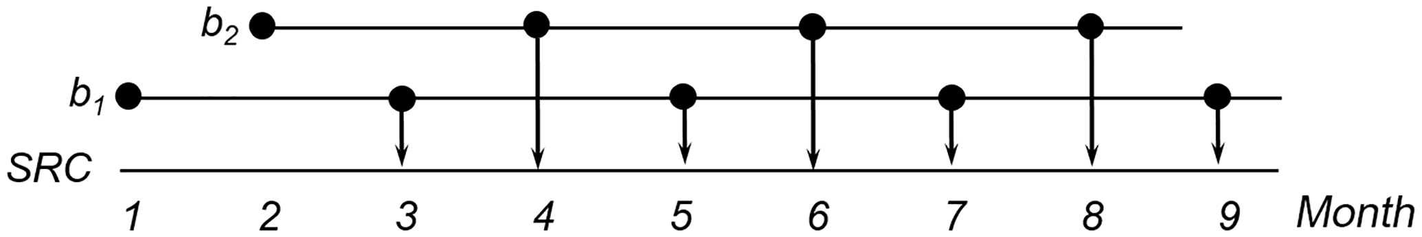
Figure 3 Schematic illustration of MAIAC dynamic SRC retrievals featuring two independent lines of update, b₁ and b₂.

The land surface is considerably brighter at 2.13 µm compared to the blue wavelength. This results in spectral dependence of the BRDF shape: when the surface is dark, the BRDF is well defined by the first order of scattering, whereas in case of a bright surface, the photon can experience several scatterings on microfacets of the surface roughness before escaping into the atmosphere, which results in relative flattening of the BRDF shape. For this reason, SRC depends on the view geometry. To account for that, MAIAC SRC is computed for three angular bins carefully selected to optimize aerosol retrievals over bright deserts where the AOD error sensitivity is maximal. Current bins represent forward scattering ($\mathit{\varphi }\le \mathrm{90}{}^{\circ }$), backscattering (μ<0.95, $\mathit{\varphi }>\mathrm{90}{}^{\circ }$) and nadir direction ($\mathrm{0.95}<\mathit{\mu }\le \mathrm{1}$, $\mathit{\varphi }>\mathrm{90}{}^{\circ }$). The latter is introduced to represent regions of the land hotspot for tropics/subtropics and near-nadir views when the sun is near zenith. A linear interpolation between bins is used within $\mathrm{\Delta }\mathit{\mu }\le \pm \mathrm{0.01}$ of bin boundaries.

Before using the LER model, we studied the full radiative transfer with anisotropic surface model where SRC is used to predict the blue-band BRDF from the BRDF at 2.13 µm. That approach was computationally more expensive and still required angular binning of SRC. Besides, we found that it was also sensitive to the B7 BRDF errors over bright surfaces, occasionally producing AOD outliers. Over bright surfaces, small errors in the BRDF shape at 2.1 µm can result in relatively large errors in the surface-reflected diffuse radiance because of high values of the BRDF shape parameters (k_v, k_g). The BRDF errors can arise from uncertainties of gridding, limitations of the RTLS model (not exactly matching the real distribution), or rarely, unstable RTLS inversions. Using only TOA measurements at two wavelengths, the LER approach eliminates uncertainty from the BRDF model-based sources and provides a more stable AOD retrieval with better AERONET comparison. The current C6 MAIAC uses the LER surface model for both SRC and aerosol retrievals.

6 Aerosol retrievals

6.1 Aerosol models

The geographic distribution of regional background aerosol models over land used in MAIAC processing is shown in Fig. 4. MAIAC uses eight different models listed in Table 1. Model properties are given in terms of volumetric size distribution (e.g., Dubovik and King, 2000) with radius (R_v) and standard deviation (σ_v) for the fine and coarse modes, their ratio of concentrations ($C_{\mathrm{v}}^{\mathrm{C}}/C_{\mathrm{v}}^{\mathrm{F}})$, real (m) and imaginary (k) refractive index, absorption Ångström exponent (AAE) defined with respect to spectral dependence of k and spherical (Mie) aerosol fraction. The imaginary refractive index is assumed to be spectrally dependent at $\mathit{\lambda }<{\mathit{\lambda }}_{\mathrm{0}}=\mathrm{0.66}\mathrm{\mu }\mathrm{m},k\left(\mathit{\lambda }\right)=k\left({\mathit{\lambda }}_{\mathrm{0}}\right)(\mathit{\lambda }/{\mathit{\lambda }}_{\mathrm{0}}{)}^{-\mathrm{AAE}}$ and constant for longer wavelengths. The aerosol models can be either static with fixed parameters, typical of an arid environment, or dynamic (Remer and Kaufman, 1998) with parameters depending on AOD. Growth of volumetric radius with AOD represents hygroscopic growth of aerosol particles associated with AOD increase. It is typical for regions with moderate-to-high humidity. Model parameters (size distribution, ratio of volumetric concentrations, refractive index) are generally representative of the AERONET regional climatology (e.g., Dubovik et al., 2002) with empirical adjustments aimed at achieving a better match of retrieved AOD to AERONET sun-photometer data.

Table 1 Microphysical properties of MAIAC aerosol models: radius and standard deviation of fine and coarse fractions of bi-lognormal volume size distribution; ratio of volume concentrations (coarse to fine) as functions of AOD (τ); real and imaginary refractive index (n= m-ik); Ångström (AAE) parameter for k ($k\left(\mathit{\lambda }\right)=k\left({\mathit{\lambda }}_{\mathrm{0}}\right)(\mathit{\lambda }/{\mathit{\lambda }}_{\mathrm{0}}{)}^{-b}$, for $\mathit{\lambda }<{\mathit{\lambda }}_{\mathrm{0}}=\mathrm{0.66}$ µm and k(λ)=k(λ₀) for λ>λ₀). Finally, the last column shows the fraction of spherical particles where 1 represents spheres and 0 represent spheroids from the DLS model (Dubovik et al., 2006).

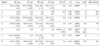
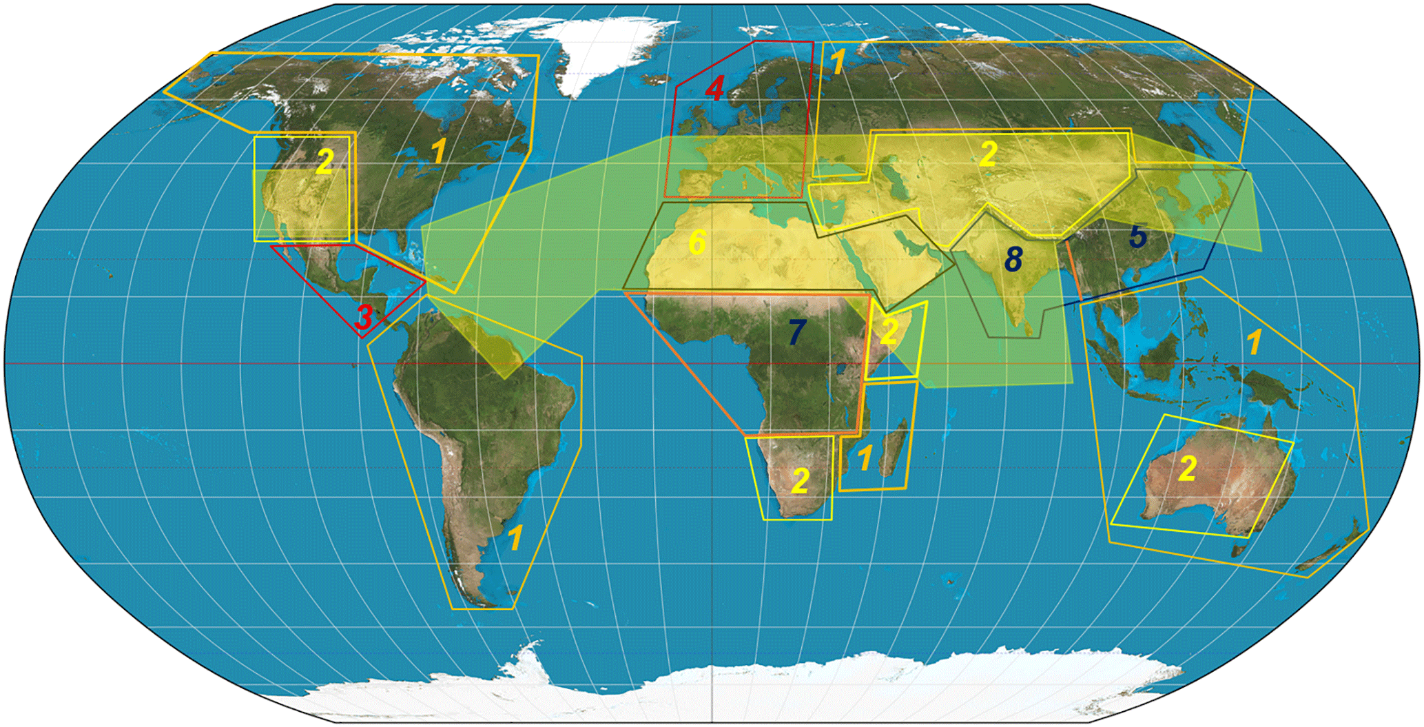
Figure 4 Map of background regional aerosol models specified in Table 1. The transparent yellow shape approximates the dust regions.

Dynamic Model 1, based on the GSFC AERONET site, represents east coast USA with high summertime humidity. The more arid climate of the western USA is represented by Model 2, with some contribution of dust particles and larger coarse fraction. Model 3, which has high absorption, was developed to model the polluted environment of Mexico City. The European Model 4 has a higher absorption, but otherwise is the same as the east coast USA model, Model 1. Model 5, representing industrial-world China, was developed based on the Beijing AERONET model with an adjustment for absorption. The India model, Model 8 is similar to 5 but with higher absorption coming from agricultural biomass burning (seasonal), cooking and transportation (e.g., Singh et al., 2017). The biomass-burning cerrado model (Model 7) of subequatorial Africa was developed based on a AERONET Mongu site. Finally, the desert dust model (Model 6) was based on Dubovik et al. (2002) climatological model for the Solar Village site.

The transparent yellow shape in Fig. 4 maps the world region in which the dust test is conducted and AOD is retrieved with the background or the dust model depending on the dust test outcome. In the MAIAC C6 version, we still use the regional background model for aerosol retrieval and atmospheric correction even if smoke was detected. The next version will use a joint AOD–SSA (single-scattering albedo) retrieval algorithm for areas with detected smoke. This algorithm has already been developed and is in the testing/tuning phase.

Lack of seasonal dependence of aerosol models and LUTs is one of the limitations of MAIAC C6. It does not account for regional aerosol seasonality, for instance periods of biomass burning and variations in humidity. As a result, current AOD product may show seasonal biases, for instance over India during post-monsoon biomass burning (Mhawish et al., 2018). This issue will be fixed in the next version of MAIAC.

6.2 Aerosol algorithm

The aerosol algorithm depends on the brightness of surface, which is characterized using the uncertainty parameter δτ^a. Over dark surfaces ($\mathrm{0}\le \mathit{\delta }{\mathit{\tau }}^a<\mathrm{0.05}$), the AOD retrieval routine first evaluates LER in B3 (0.47 µm):

$$\begin{array}{}\text{(10)}& {\mathit{\rho }}_{\mathrm{0.47}}=b_{\mathrm{37}}{\mathit{\rho }}_{\mathrm{2.13}},\end{array}$$

and then computes AOD by matching the LUT-based theoretical reflectance to the measurement,

$$\begin{array}{}\text{(11)}& R_{\mathrm{0.47}}^{\mathrm{T}}\left({\mathit{\tau }}^a\right)=R_{\mathrm{0.47}}^{\mathrm{M}}.\end{array}$$

The LER ρ_2.13 is obtained by atmospheric correction from the measurement $R_{\mathrm{2.13}}^{\mathrm{M}}$ with current AOD used in the aerosol retrieval loop. However, when smoke/dust is detected, or LER ρ_2.13 is significantly different from the BRDF model value, ρ_2.13<0.5RTLS_2.13 or ${\mathit{\rho }}_{\mathrm{2.13}}>\mathrm{2}{\mathrm{RTLS}}_{\mathrm{2.13}}({\mathit{\rho }}_{\mathrm{2.13}}>\mathrm{1.5}{\mathrm{RTLS}}_{\mathrm{2.13}}$ for bright surfaces when $k_{\mathrm{2.13}}^L>\mathrm{0.25}$), which usually indicates undetected clouds or cloud shadows, we use the BRDF model as LER, ρ_2.13=RTLS_2.13.

The dark target algorithm (Levy et al., 2013) is prone to overestimating AOD as surface brightness increases. A typical example of high bias in the VIIRS aerosol algorithm is given by Fig. 7d from Superczinsky et al. (2017). While MAIAC implementation is different from the VIIRS (Jackson et al., 2013), it faces the same general issue. Over brighter surfaces, as sensitivity of measurements to AOD decreases, the effect of the surface-related errors increases. The surface-related errors include those from gridding, from the lagged SRC characterization with the time series method, etc. Over bright land, the SRC error, essentially related to the change in the average sun angle during the 2-month lag period, becomes more important over mountainous regions with terrain slope variations. Statistically, most surface-related errors, including those from gridding, should be symmetric about zero. However, because we do not accept negative AOD, the net effect is a positive bias.

One more error source is characterization of the angular dependence of SRC. As surface brightness increases, the difference in the BRDF shape between darker 0.47 and much brighter 2.13 µm channels (angular dependence of SRC) increases. To reduce this effect, we added minimization of the blue∕green band ratio where the surface brightness and BRDF shapes are much closer. The resulting AOD retrieval is based on minimization of the following function:

$$\begin{array}{ll}{\displaystyle }F\left({\mathit{\tau }}^a\right)& {\displaystyle }=w_{\mathrm{1}}(\mathrm{1}-R_{\mathrm{0.47}}^{\mathrm{T}}({\mathit{\tau }}^a)/R_{\mathrm{0.47}}^{\mathrm{M}}{)}^{\mathrm{2}}+w_{\mathrm{2}}(\mathrm{1}-\left[{\mathit{\rho }}_{\mathrm{0.47}}\right({\mathit{\tau }}^a)\\ \text{(12)}& {\displaystyle }& {\displaystyle }/{\mathit{\rho }}_{\mathrm{0.55}}\left({\mathit{\tau }}^a\right)]/b_{\mathrm{34}}{)}^{\mathrm{2}},\end{array}$$

where the weights of B3/B7 0.47–2.13 µm (w₁) and of B3/B4 0.47–0.55 µm ($w_{\mathrm{2}}=\mathrm{1}-w_{\mathrm{1}})$ are functions of surface brightness expressed via uncertainty δτ^a (Eq. 6) as follows: w₁=1 if $\mathrm{0}\le \mathit{\delta }{\mathit{\tau }}^a<\mathrm{0.05}$ (dark surface), w₁=0 if δτ^a<0 or δτ^a>0.5 (bright surface) and a linear function in between, $w_{\mathrm{1}}=(\mathit{\delta }{\mathit{\tau }}^a-\mathrm{0.05})/\mathrm{0.45}$. The reflectance ρ_λ(τ^a) in Eq. (12) is LER (result of atmospheric correction) with AOD τ^a. The minimization algorithm (Eq. 12) incrementally increases AOD from the LUT until F(τ^a) reaches minimum, computes coefficients of quadratic polynomial based on three points encompassing the minimum and analytically computes AOD in the minimum of quadratic function.

Our study of independent AOD retrievals using 0.47–0.55 µm ratio (second term of Eq. 12) shows that it (1) has reasonable accuracy over dark surfaces albeit somewhat lower than the standard algorithm (Eqs. 10–11), (2) is more stable over bright surfaces with zero or much lower positive AOD bias when atmospheric AOD is low and (3) underestimates AOD at high aerosol loading over all surfaces by as much as 20 %–50 %. Given these properties, it is clear that the second term of Eq. (12), having lower sensitivity to AOD, mostly serves to stabilize the solution over brighter surfaces under clean (low AOD) atmospheric conditions by minimizing high AOD bias from the first term.

When smoke is detected, meaning that AOD is usually sufficiently high and effect of surface errors is reduced, we give more weight (if w₁<0.8 then w₁=0.8) to the standard retrieval (bands B3–B7) with much higher sensitivity to AOD.

Finally, when dust is detected, the aerosol retrieval adds an additional term for the MODIS red band B1 and uses equal weights for all three terms:

$$\begin{array}{ll}{\displaystyle }F\left({\mathit{\tau }}^a\right)& {\displaystyle }={\left(\mathrm{1}-R_{\mathrm{0.47}}^{\mathrm{T}}\left({\mathit{\tau }}^a\right)/R_{\mathrm{0.47}}^{\mathrm{M}}\right)}^{\mathrm{2}}+\left(\mathrm{1}-\left[{\mathit{\rho }}_{\mathrm{0.47}}\left({\mathit{\tau }}^a\right)\right.\right.\\ \text{(13)}& {\displaystyle }& {\displaystyle }{\left.\left./{\mathit{\rho }}_{\mathrm{0.55}}\left({\mathit{\tau }}^a\right)\right]/b_{\mathrm{34}}\right)}^{\mathrm{2}}+{\left(\mathrm{1}-R_{\mathrm{0.64}}^{\mathrm{T}}\left({\mathit{\tau }}^a\right)/R_{\mathrm{0.64}}^{\mathrm{M}}\right)}^{\mathrm{2}}.\end{array}$$

The theoretical B1 TOA reflectance in the last term is computed using the accurate GF solution (Eq. 2) with the B1 BRDF model. As one can see from Table 1, properties of the dynamic dust model are such that the concentration of the coarse mode rapidly grows with AOD, increasing the anisotropy of the phase function and reducing backscattering. This reduction counteracts and slows down the respective increase of TOA reflectance. In effect, the dynamic Model 6 requires a significantly higher AOD to match the measured reflectance at 0.47 µm. We found experimentally that algorithm (Eq. 12) significantly overestimates dust AOD by up to a factor of 2. However, adding the red-band term (Eq. 13) reduces AOD and significantly improves its accuracy. The mentioned spectral imbalance of the dust Model 6 may be caused by our use of the spheroidal model (Dubovik et al., 2006) to approximate dust particles. A similar spectral-angular mismatch from the use of spheroids to describe optics of the dust scattering was observed in the analysis of MISR data (Ralph Kahn, personal communication, 2018).

Lastly, at high altitudes (H>4.2 km, e.g., Tibetan plateau), AOD is not retrieved unless smoke/dust was detected. Our study shows that in conditions of very low AOD, nonflat terrain and a generally bright surface, MAIAC aerosol retrievals at high altitudes are unreliable. Instead of retrievals, we assume a fixed climatology AOD_min=0.02 for the atmospheric correction.

6.3 Bright surface bias correction

Regardless of the specific AOD retrieval algorithm, solutions over bright surfaces can be unstable and can easily develop a positive bias. It should be mentioned that the term “bright surface” in MAIAC is understood in terms of low sensitivity ($\partial R/\partial {\mathit{\tau }}^a\sim \mathrm{0}$) or high uncertainty (δτ^a) of aerosol retrievals. The same surface can be bright in the backscattering directions, in particular close to the hotspot because of an increase in the surface reflectance, and dark for the forward-scattering geometries where the surface is considerably darker due to shadowing, in combination with higher aerosol phase function and the single-scattering radiance. MAIAC retrievals show that AOD is systematically overestimated over some bright surfaces in the backscattering view directions, correlating with the surface features, which is apparent in the time series of gridded AOD. These artifacts are generic and one can easily find them in the MODIS DT, DB and in the VIIRS aerosol products. As MAIAC deals with the time series analysis of gridded data directly, we developed a special statistical correction procedure. It is designed to detect and minimize spatially persistent biases and is only applied in clear low-AOD conditions to prevent canceling the real aerosol signal. The idea is to look at the large area, evaluate an average AOD using the darkest pixels for which the solution can be trusted and correct biased AOD over bright pixels with a known history of bias using the area-average value.

The bright surface correction procedure is applied to mesoscale areas (150×150 km²), denoted by Ṙ below, and works as follows:

1. Compute average AOD for pixels in four bins of uncertainty: δτ^a≤0.05f, $\mathrm{0.05}<\mathit{\delta }{\mathit{\tau }}^a\le \mathrm{0.12}f$, 0.12<δτ^a≤0.22f and 0.22<δτ^a≤0.4f. The AOD retrieval is trustworthy in the first bin and usually trustworthy in the second bin. The first two bins cover densely vegetated surfaces and dark soils, but extend to considerably (visually) brighter surfaces at low sun/view zenith angles and/or high atmospheric turbidity.

2. The AOD bias generally manifests itself as an increase in the average AOD with the bin number (uncertainty). In such a case, we define the area-average value τ_av based on the first bin or the first two bins depending on the statistics (the number of pixels in these bins) and set the high AOD threshold as thresh $={\mathit{\tau }}_{\mathrm{av}}+\mathrm{0.1}$.

3. Mask the pixel in the high bins 2–4 if its AOD (τ_ij) exceeds the threshold. When a pixel is masked, its cumulative bias counter (q.indexHighBias) is increased by 1, and the bias index for the current observation (q.indexCurrentBias) is set to 1.

4. For pixel (i,j) with current and persistent high bias (q.indexCurrentBias = 1 and q.indexHighBias > 2), replace AOD with the value ${\mathit{\tau }}_{ij}w+{\mathit{\tau }}_{\mathrm{av}}(\mathrm{1}-w)$, where the weight increases along with the deviation of pixel's AOD from the average, $w=({\mathit{\tau }}_{ij}/{\mathit{\tau }}_{\mathrm{av}}{)}^{-\mathrm{2}}\le \mathrm{1}$.

   The above procedure is not applied when absorbing aerosols (smoke/dust) are detected or when τ_av>0.3, indicating the possibility of generally higher aerosol levels.

5. Finally, it should be mentioned that the bias detection can be triggered randomly for almost any pixel, leading to the accumulation of noise in the cumulative counter. For this reason, and to avoid canceling the real aerosol signal over regular pixels, we compute the average bias detection noise over area Ṙ and subtract it from q.indexHighBias monthly, effectively zeroing it for the regular pixels.

It should be mentioned that the described algorithm is largely an empirical summary of numerous trials and errors using AERONET validation and minimization of systematic spatial and temporal artifacts as our main criteria.

7 Spatial AOD filtering and smoothing

Cloud tests (Sect. 4) were designed to capture reliable bright, cold, high, or spatially/spectrally contrasting clouds. Because the natural transition from clear to cloudy is on a continuum, we use two additional AOD-based filters to detect thin or subpixel clouds at 1 km resolution, all based on an assumption that aerosols have some degree of spatial homogeneity. The filters below were not used if absorbing aerosols (smoke/dust) were detected.

1. The first filter uses a histogram-based technique following the DT algorithm (Levy et al., 2007), which applies it to the TOA reflectance in 20×20 500 m pixels' boxes, filtering the lower 20 % and upper 50 % of data as potentially affected by either shadows or clouds. The average reflectance of the remaining pixels is used for the DT AOD retrieval. In MAIAC, we apply a similar technique to 25×25 km² blocks by using retrieved AOD and by filtering high values only. The upper threshold is a function of the cloud fraction (CF) in the block, $H=\mathrm{0.65}-\mathrm{0.6}\mathrm{CF}/\mathrm{0.9}$, decreasing from 65 % in cloud-free conditions to 5 % when CF=0.9. The AOD threshold is defined as thresh = AOD_H+δ, where δ=0.2 when covariance is high (q.iFlag_HighCov = 1), and δ=0.1 otherwise. For pixels with AOD > thresh, the cloud mask value is set to possibly cloud, CM_PCLOUD.

   This filter is not applied when absorbing aerosols (smoke/dust) were detected, as well as in clear (AOD_max<0.35) or homogeneous (AOD${}_{\max }-{\mathrm{AOD}}_{\min }<\mathrm{0.2}$) conditions. Overall, this filter rather significantly improves the quality of the final AOD product.

   In earlier versions, AOD for the filtered pixels was set to the FILL_VALUE. The current C6 version reports retrieved AOD for these pixels for possible applications as a research quality. The main impetus came from the air quality research groups: in particular, I. Kloog and A. Just showed that the histogram filter often cancels AOD retrievals over urban regions with high aerosol spatial variability from human activity, e.g., the southwestern part of Mexico City. AERONET validation for Mexico City shows an improvement from added high AOD pixels which were previously mostly filtered as CM_PCLOUD. A similar improvement was observed at the Ispra (Italy) AERONET site, located on western edge of the Po Valley, Italy, where topography and proximity of aerosol emission sources create conditions for high spatial aerosol variability.

   Most of the CM_PCLOUD pixels are located in the transition zone from clear to confidently cloudy. The high 1 km resolution AOD in this twilight region (Koren et al., 2007) may be useful for studying the aerosol–cloud interactions. However, we should emphasize that for most applications, the user should only use the highest quality AOD with QA cloud mask value CM_CLEAR.

2. The second spatial homogeneity filter based on the analysis of 3×3 pixels was proposed by Emili et al. (2011). We use it in the following form:

   • find pixel with maximum AOD over 3×3 pixels (AOD_max),

   • compute average AOD_av in 3×3 area without this pixel,

   • filter the maximum value (CM_PCLOUD) if AOD${}_{\max }>{\mathrm{AOD}}_{\mathrm{av}}+\mathrm{0.2}$.

   After detection of residual clouds with filters 1–2, a 3×3 running averaging window is applied to 1 km AOD, except when smoke/dust were detected. The averaging serves to ameliorate residual errors of gridding, which create noise in the surface SRC, BRDF and AOD. As this noise is local and spatially coherent (due to the systematic nature of MODIS orbits and footprint size/location with the scan angle), it is effectively reduced by the 3×3 smoothing filter.

8 Cloud shadow detection

With cloud detection completed, the next step (7) detects cloud shadows using geometric analysis (Simpson et al., 2000) and a BRDF reduction test. Based on the view geometry, we generate the line of shadow for each cloudy pixel, which is a function of the cloud top height (H_c). Parameter H_c is evaluated based on the Tb₁₁ contrast between the cloud-free background (q.Tb_s) and a cloudy pixel, assuming an average adiabatic lapse rate of 6.5^∘ K∕km ($H_{\mathrm{c}}=({\mathrm{Tb}}_{\mathrm{11}}-\mathrm{q}.{\mathrm{Tb}}_s)/\mathrm{6.5}$). If the background brightness temperature cannot be reliably evaluated, we assume a maximal cloud height of 12 km (Stubenrauch et al., 2010). The shadow is detected along the line of shadow if surface reflectance in the bright channels B2 (0.87 µm) or B5 (1.24 µm) falls below the BRDF-predicted value by a certain threshold. Based on visual evaluation, the developed approach captures up to 80 %–90 % of cloud shadows.

9 Atmospheric correction

Following cloud detection and aerosol retrieval, the atmospheric correction derives surface spectral BRF and BRDF models, and computes instantaneous albedo. The spectral BRF is derived for cloud-free and clear to moderately hazy (AOD_0.47<1.5) pixels by scaling a pixel's BRDF in order to match the TOA reflectance (Lyapustin et al., 2012a). It uses Eq. (2) modified as follows:

$$\begin{array}{}\text{(14)}& R({\mathit{\mu }}_{\mathrm{0}},\mathit{\mu },\mathit{\varphi })=R^{\mathrm{A}}({\mathit{\mu }}_{\mathrm{0}},\mathit{\mu },\mathit{\varphi })+c{R}^{\mathrm{Surf}}({\mathit{\mu }}_{\mathrm{0}},\mathit{\mu },\mathit{\varphi }),\end{array}$$

where R^Surf is a surface-reflected term computed using the current RTLS parameters and retrieved aerosol data, and c is the spectrally dependent scaling factor. Then, the BRF is given by the following:

$$\begin{array}{}\text{(15)}& r_{\mathit{\lambda }}({\mathit{\mu }}_{\mathrm{0}},\mathit{\mu },\mathit{\varphi })=c_{\mathit{\lambda }}{\mathit{\rho }}_{\mathit{\lambda }}({\mathit{\mu }}_{\mathrm{0}},\mathit{\mu },\mathit{\varphi }),\end{array}$$

where ρ_λ is computed from the RTLS model for a given geometry. Because R^Surf is a nonlinear function of the surface reflectance, solving Eqs. (14) and (15) takes two iterations. On the second iteration, the surface term R^Surf is computed with scaled BRDF from the first iteration, $c_{\mathit{\lambda }}^{\left(\mathrm{1}\right)}{\mathit{\rho }}_{\mathit{\lambda }}({\mathit{\mu }}_{\mathrm{0}},\mathit{\mu },\mathit{\varphi })$, and the final scaling coefficient in Eq. (15) is a product $c_{\mathit{\lambda }}=c_{\mathit{\lambda }}^{\left(\mathrm{1}\right)}{c}_{\mathit{\lambda }}^{\left(\mathrm{2}\right)}$. Because the nonlinearity is small, the second iteration has a very small effect on the final result Eq. (15).

In addition to 1 km spectral BRF in MODIS bands 1–7 is also computed at 500 m resolution nested in a 1 km grid. While MAIAC performs atmospheric correction of MODIS 250 m bands (B1–B2) as well, these results are not currently included in the output files.

The RTLS model parameters are retrieved for bands B1–B8 only. Therefore, BRF in MODIS ocean bands B9–B12 is computed with the same approach (Eqs. 14–15) using BRDF from the nearest bands; for instance, B4 BRDF is used for B11–B12. The red band B1 BRDF (instead of B3) is used for AC of B9–B10 in the blue part of the spectrum. Over dense vegetation, the red-band reflectance is nearly as low as that in the blue but it is significantly less affected by the aerosol retrieval errors. So, while the shapes of BRDF are very similar, the BRDF is somewhat more stable in the red. At the same time, the difference in the magnitude of reflectance does not matter for the scaling approach (Eqs. 14–15) as long as the general BRDF shape is right and correctly models the surface reflection and upward propagation for the direct solar beam and diffuse (sky) irradiance.

A Lambertian assumption is used during the algorithm initialization period, which may last from just 4 days (observations) in cloud-free low-AOD conditions to over a month depending on cloudiness and snow cover. During this period of time, MAIAC performance is suboptimal with a higher rate of undetected clouds and reflectance biases from the Lambertian assumption. In the ongoing C6 MODAPS processing of MODIS Terra and Aqua, MAIAC was initialized globally using the second half of 2002, and then the processing started from the beginning of 2000. In parallel, a separate forward-processing stream using MODIS data from the second half of 2016 to initialize is expected to start soon.

The latest BRF combined with previous BRFs stored in the queue are used for the BRDF inversion, providing three parameters of the RTLS model. This represents a change from the original algorithm (Lyapustin et al., 2012a), which derived RTLS coefficients by matching the measured TOA reflectance. Using the original TOA measurements potentially allows a better accuracy of BRDF retrievals to be achieved, but at the expense of storing or recomputing a number of RT functions for each past observation from the queue. Our analysis showed that, with the current high accuracy of MAIAC cloud detection and aerosol retrieval, the result of much simpler and faster BRF-based inversion is practically indistinguishable from the TOA-based inversion.

With a C6+ calibration (Lyapustin et al., 2014b), which added MODIS Terra polarization correction (Kwiatkowska et al., 2008) and response vs. scan (RVS) trending using quasi-stable desert calibration sites (Sun et al., 2014), and removed residual trends and cross-calibrated Terra to Aqua, we are using MODIS Terra and Aqua as one data set. This doubles the MODIS revisit frequency, a critical requirement for the time series analysis, which significantly helps MAIAC in all stages of processing, in particular for the BRDF retrieval and SRC characterization.

MAIAC has a surface change detection algorithm (Lyapustin et al., 2012a) based on an analysis of geometrically normalized BRF in bands B1, B2, B7. For instance, normalization to SZA = 45^∘ and VZA = 0^∘ ($F_{\mathrm{0}V}=-\mathrm{0.0458621}$, $F_{\mathrm{0}G}=-\mathrm{1.1068192}$ in Eq. 1) at any wavelength uses the following formula (see Eq. 6 from Lyapustin et al., 2012a):

$$\begin{array}{ll}{\displaystyle }{\mathrm{BRF}}_n=& {\displaystyle }\mathrm{BRF}\cdot (k^L-\mathrm{0.0458621}\cdot k^{\mathrm{V}}-\mathrm{1.1068192}\cdot k^{\mathrm{G}})\\ \text{(16)}& {\displaystyle }& {\displaystyle }/(k^L+F_{\mathrm{V}}\cdot k^{\mathrm{V}}+F_{\mathrm{G}}\cdot k^{\mathrm{G}}),\end{array}$$

where F_V and F_G are volumetric and geometric kernels for the MODIS view geometry provided for the user's convenience in the MAIAC output (see Sect. 10.2.2). Geometric (or BRDF) normalization significantly reduces BRF variations (by a factor of 3–6) caused by the changing view geometry of MODIS with the orbit. MAIAC change detection looks for anticorrelated changes in the red and NIR bands during the accumulation period, $\mathit{\eta }=\mathrm{\Delta }{\mathrm{BRF}}_n/{\mathrm{BRF}}_{n,\mathrm{av}}$, where BRF_n,av is an average value. Based on this analysis, the surface state is characterized as stable or having no change (η<0.05) and two categories of greenup or senescence, namely regular change ($\mathrm{0.05}<\mathit{\eta }<\mathrm{0.15}$) and big change (η>0.15, Sect. 10.2.2).

Based on extensive empirical analysis, MAIAC undertakes RTLS inversion when the surface is relatively stable, η<0.15). When change is significant (η≥0.15), the BRDF is scaled with the latest observation to adjust the total reflectance assuming the shape of BRDF does not change, as in (Schaaf et al., 2002). After inversion, the new BRDF goes through several tests to verify the correctness of its shape and its consistency with the previous solution stored in the queue (for details, see Lyapustin et al., 2012a). In order to preserve consistency and reduce random noise, we are using an update with relaxation,

$$\begin{array}{}\text{(17)}& \mathit{K}=w{\mathit{K}}^{\mathrm{new}}+(\mathrm{1}-w){\mathit{K}}^{\mathrm{prev}}.\end{array}$$

Above, the superscript indicates the new and previous solutions, the weight w=0.5 when surface does not change and w=0.7 for the regular change. While such an update practice generally improves the quality of the BRDF model during stable periods, it delays the BRDF model response to the surface change in addition to the delay related to the length of the queue. On the contrary, spectral BRF_n represents an instantaneous surface snapshot from the latest observation. For this reason, studies of vegetation phenology, seasonality, etc. should use BRF_n rather than BRDF model-based reflectance values.

Many applications, including higher-level algorithms for vegetation characterization, e.g., LAI/FPAR (Chen et al., 2017) and global model assimilation, require knowledge of uncertainty. We provide the BRF uncertainty (Sigma_BRFn) in MODIS red (B1) and NIR (B2) bands at 1 km defined as a standard deviation of the BRFn over the accumulation period of the queue (4–16 days) under the assumption that the surface is stable or changes linearly in time. This is one of the most conservative and realistic estimates of uncertainty which includes contribution from gridding, undetected clouds, errors of atmospheric correction including those from the aerosol retrieval, and of surface change when reflectance change is nonlinear over the length of the queue. Sigma_BRFn in the red band can serve as a proxy of uncertainty at shorter wavelengths, where the surface is generally darker, and the NIR value can be a proxy for the longer wavelengths with high surface reflectance.

With the detection of snow, MAIAC freezes the land spectral BRDF in the Q memory and switches to the snow processing mode, retrieving subpixel snow fraction and snow grain size. The total surface reflectance (albedo) in this case is computed as a linear mixture of land BRDF and snow reflectance given by a semi-analytical model (Lyapustin et al., 2010).

10 MCD19 data products and quality assurance

MAIAC provides a suite of MODIS atmospheric and surface products in three HDF4 files: daily MCD19A1 (spectral BRF, or surface reflectance), daily MCD19A2 (atmospheric properties) and 8-day MCD19A3 (spectral BRDF/Albedo). As this paper describes the first official public release of MAIAC MODIS data, we consider it useful to provide a brief technical description of MAIAC products and its quality assurance flags (QA) which is given in the User's Guide in more detail.

10.1 Tiled file structure and naming convention

All products are reported on 1 km sinusoidal grid. The sinusoidal projection is not optimal due to distortions at high latitudes and off the grid center, but it is a tradeoff made by the MODIS Land team for the global data processing. The gridded data are divided into 1200×1200 km² standard MODIS tiles shown in Fig. 5. The current data set presents data per orbit. Each daily file name follows the standard MODIS name convention, for instance:

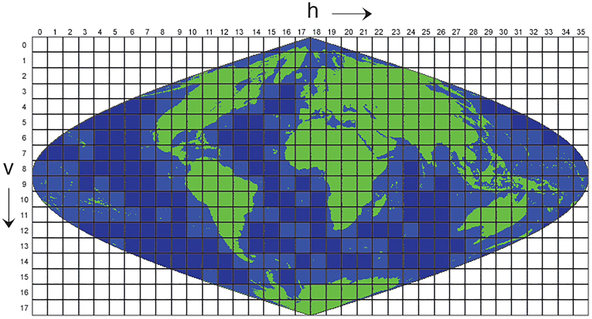
Figure 5 Illustration of MODIS tiles for the sinusoidal grid. MAIAC performs processing over green and light blue (land-containing) tiles.

MCD19A1.DayOfObservation.TileNumber.Collection. TimeOfCreation.hdf. DayOfObservation has the format YYYYDDD, where YYYY is year, DDD is Julian day. TileNumber has the standard format, e.g., h11v05 for the east coast USA.

Each daily file usually contains multiple orbit overpasses (1–2 at equator and up to 30 in the polar regions for combined Terra and Aqua) which represents the third (time) dimension of MAIAC daily files. The orbit number and the overpass time of each orbit are saved in global attributes “Orbit_amount” and “Orbit_time_stamp” sequentially. The Orbit_time_stamp has the format YYYYDDDHHMM[TA], where YYYY is year, DDD is Julian day, HH is hour, MM is minute, and T and A stand for Terra and Aqua. At high latitudes, only 16 orbits with the largest coverage are reported per day in order to limit the file size.

10.2 MAIAC products: general description

MAIAC conducts processing over global land tiles and land-containing ocean tiles (green and light blue colors in Fig. 5).

Over inland, coastal and open-ocean waters, MAIAC reports AOD, fine-mode fraction and spectral reflectance of underlight (water-leaving radiance). MAIAC processing over water will be described in a separate publication.

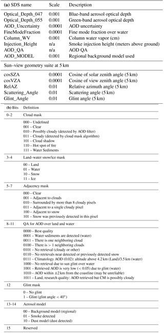
10.2.1 Atmospheric properties file (MCD19A2)

For each orbit, the MAIAC daily MCD19A2 (atmospheric properties) file includes the following parameters listed in Table 2a. Over land, MAIAC reports the following parameters at 1 km resolution: AOD at 0.47 and 0.55 µm and AOD uncertainty evaluated using Eq. (9) for cloud-free and possibly cloudy pixels; column water vapor (cm) for all pixels; injection height of smoke plume (in meters above ground); and background aerosol model used in the retrievals (see Fig. 4). The aerosol type (result of smoke/dust test) is reported in QA bits 13–14 (aerosol model) of Table 2b.

Table 2 (a) Reported parameters in the atmospheric properties file (MCD19A2). (b) AOD QA definition for MCD19A2 (16 bit unsigned integer). N/a is not applicable.

Over water, we report AOD outside of the glint area. Current processing has a glint angle cutoff of $\le \mathrm{40}{}^{\circ }$ as in the DT-over-ocean algorithm (Levy et al., 2013). When MAIAC detects dust, AOD is also reported for smaller glint angles when measured TOA reflectance at 1.24 µm (B5) significantly exceeds reflectance from the ocean surface predicted by the Cox–Munk model (Cox and Munk, 1954) for a given wind speed. Over the open ocean and large inland lakes (e.g., Great Lakes of North America), we also report the fine-mode fraction (FMF). FMF is not retrieved over small inland water bodies.

In addition to the blue-band AOD (0.47 µm), MAIAC also reports AOD at 0.55 µm, which is computed based on spectral properties of the aerosol model used in retrievals. It is provided to support the regional and global chemical transport and climate simulation models, AOD validation and AOD product intercomparison, all standardized to 0.55 µm. Validation shows that the quality of AOD at 0.55 µm is generally close though slightly worse than the original retrieval at 0.47 µm.

Along with the retrieval results, we also provide the sun–view geometry at 5 km resolution, which includes cosines of solar and view zenith angle, relative azimuth, and scattering and glint angles, which may be required for analysis or applications.

The QA structure for MCD19A2 file is presented in Table 2b.

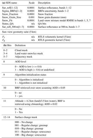
10.2.2 Surface reflectance file (MCD19A1)

For each orbit, the MAIAC daily MCD19A1 (surface reflectance) file includes parameters shown in Table 3a.

Over cloud-free land and clear-to-moderately turbid (AOD_0.47<1.5) conditions, for solar zenith angles below 80^∘, file MCD19A1 reports the surface BRF at 1 km in bands 1–12, and at 500 m in bands 1–7 and BRF uncertainty (Sigma_BRFn) in MODIS red (B1) and NIR (B2) bands at 1 km. When snow is detected, we report snow grain size (diameter in millimeters), subpixel snow fraction and RMSE (Snow_Fit) between MODIS measurements in bands B1, B5, B7 and the linear mixture model of spectral snow reflectance and land spectral BRDF at 1 km. Following the sun–view geometry suite at 5 km, MCD19A1 also reports values of volumetric (F_v) and geometric-optics (F_g) kernels of the RTLS model for the geometry of observation. The kernels are provided for the ease of users' geometric (or BRDF) normalization of spectral BRFs using Eq. (16). One can easily modify normalization to a preferable sun angle according to latitude or season, by replacing coefficients in the numerator of Eq. (16) with values from Table 1 in the User's Guide calculated for different solar zenith angles and nadir view.

Table 3 (a) Reported parameters in the surface reflectance file (MCD19A1). (b) Surface reflectance QA definition for MCD19A2 (16 bit unsigned integer).

Over water, MCD19A1 reports diffuse reflectance of underlight (of water-leaving radiance) in bands 1–12.

Table 3b shows the QA definition for the surface reflectance file. Bits 0–2, 3–4 and 5–7 are the same as in Table 2b. The QA bits 8 and 9 carry additional information about the quality of atmospheric correction. For instance, better quality is achieved at low AOD and when the surface BRDF is known (algorithm is initialized) as opposed to high AOD and/or “not initialized” status when a Lambertian assumption is used in the atmospheric correction.

10.2.3 Surface BRDF file (MCD19A3)

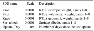
The 8-day MCD19A3 (BRDF/Albedo) file reports parameters of RTLS BRDF model (k_L, k_v, k_G) for MODIS bands B1–B8, number of days since the last RTLS model update (Update_Day) and instantaneous surface albedo for the overpass time in bands 1–8 at 1 km resolution. These parameters are listed in Table 4.

Table 4 Eight-day BRDF model parameters (MCD19A3).

10.3 Quality assurance

In daily output files, the QA reports cloud mask, adjacency mask, surface type (the result of MAIAC dynamic land–water–snow classification) and a surface change mask. In general, MAIAC aerosol–surface retrievals are only performed for cloud-free pixels (QA.Cloud_Mask = Clear) except AOD which is also reported for the value possibly cloudy. As discussed in Sect. 7, this AOD may be used with caution in specific well-understood cases, e.g., at high spatial variability of aerosol or aerosol analysis near clouds. Because most pixels with QA.Cloud_Mask = possibly cloudy contain residual cloud contamination, these pixels are not recommended for general use.

Table 5 Regional linear regression model parameters for the expected error (RMSE) and bias. NA and SA stand for North and South America.

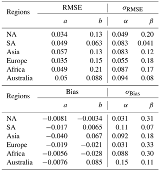
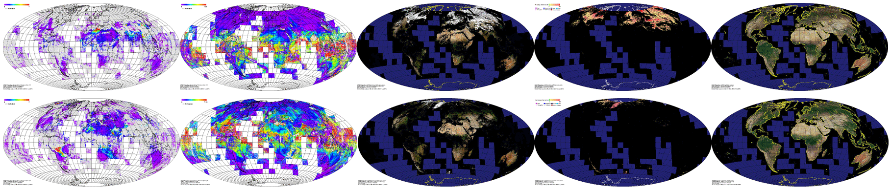
Figure 6 Global browse images showing MAIAC AOD (scale 0–2), column water vapor (scale 0–5 cm), RGB BRF, snow fraction (scale 0–1) and RGB of the isotropic parameter (k^L) of the RTLS model for days 60 (top row) and 230 (bottom row) of 2005.

Adjacency mask gives information about detected clouds or snow in the ±2-pixel vicinity. For most applications, we recommend to only use data with QA.AdjacencyMask = Clear (000). The value 011 (Adjacent to a single cloudy pixel) can also be used as it often represents a false cloud detection. The other categories of Q.AdjacencyMask are not recommended when using either AOD or BRF products because neighboring clouds or snow increase possibility of residual cloud/snow contamination of a given pixel, resulting in overestimation of AOD and respective errors of atmospheric correction.

To select the best-quality AOD, one should use QA.QA_AOD = Best_Quality which combines the best values of cloud and adjacency masks: QA.CloudMask = Clear and QA.AdjacencyMask = Clear.

For the best-quality BRF, one should apply the following QA filter: QA.AODLevel = low (0), QA.AdjacencyMask = Clear, and QA.AlgorithmInitializeStatus = initialized (0). We should admit that the current QA structure is not optimal and may be improved in the future.

10.4 An example of MAIAC products

To illustrate MAIAC product suite, Fig. 6 shows the global daily composite browse images at 20 km resolution for selected products including AOD (0–2), column water vapor (0–5 cm), RGB BRF, snow fraction (0–1) and RGB of the isotropic parameter (k^L) of the RTLS model, which gives an indication of spectral BRDF and serves as a proxy of the general surface brightness and spectral albedo. The numbers in parenthesis give the scale range. The browse images were generated by the MODAPS Land processing team (Roy et al., 2002) as part of the product quality evaluation.

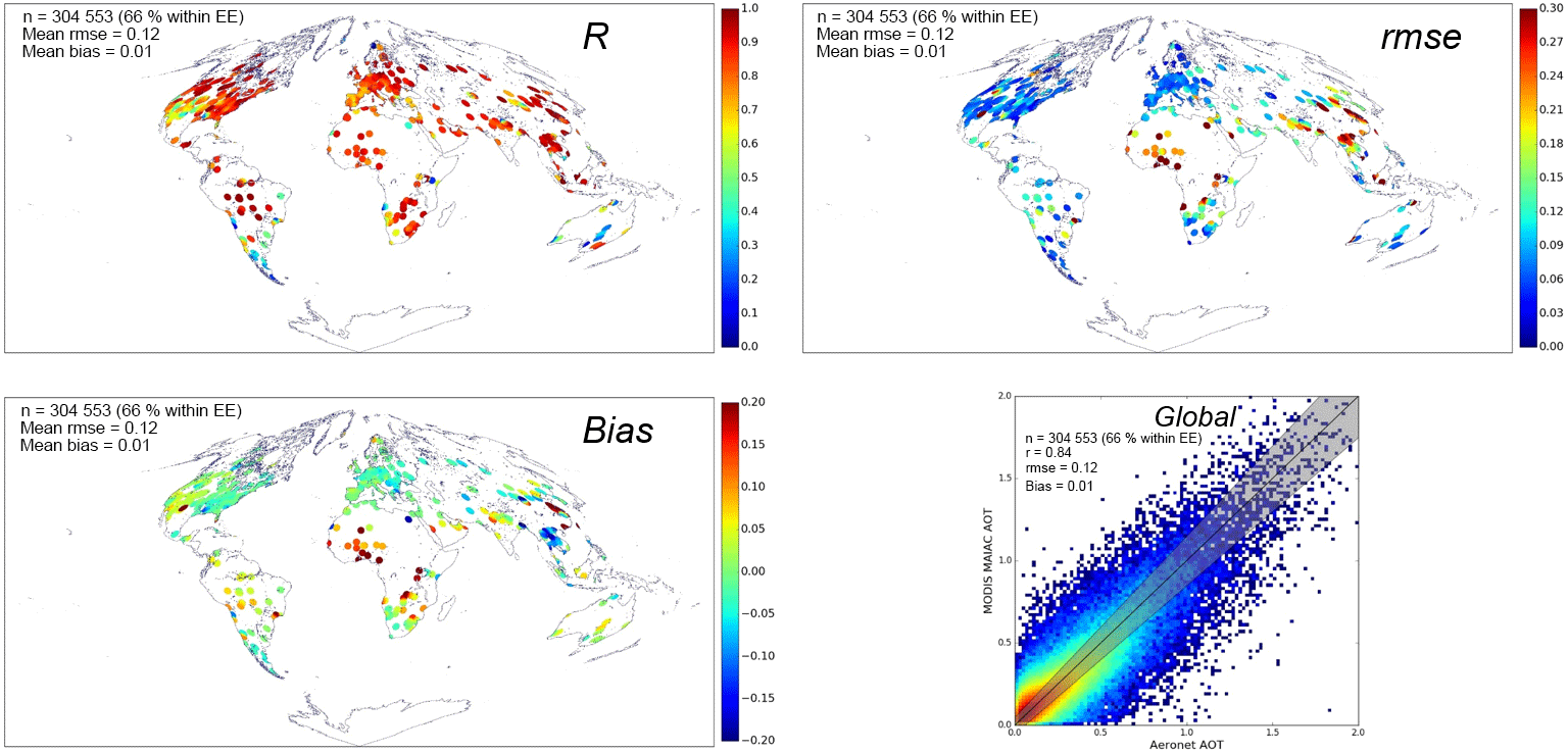
Figure 7 Results of global MAIAC AOD validation against AERONET from the MODIS Terra and Aqua 2000–2016 record.

The browse images are shown for days 60 and 230 of 2005: day 60 shows a considerable snow cover in the Northern Hemisphere in RGB BRF with the corresponding high snow fraction; dust storms in the northern Sahara and in Taklamakan Desert, and high AOD levels in the Indo-Gangetic plane, northern China and southeastern Asia. In contrast, on day 230 cloud-free observations show detected snow only over Greenland and polar north, as well as southern Andes. AOD shows strong forest fires in Alaska and large-scale biomass burning in southern Amazon with smoke transported southeast across South America. It also reveals dust storms in Western Sahara and the Thar Desert, and high aerosol levels in southern Africa. The RGB of RTLS k^L parameter is naturally gap-filled and shows contrasting seasonal dynamics of vegetation between the northern and southern hemispheres. The column water vapor shows seasonal, latitudinal and vertical variations, the latter of which is associated with retrievals above the clouds.

10.5 Accuracy assessment of MAIAC AOD

Figure 7 presents results of the global MAIAC AOD validation against AERONET (Holben et al., 1998) showing correlation coefficient, average bias and RMSE for individual AERONET sites along with the global scatterplot during 2000–2016. The detailed validation analysis of MAIAC data set, and its comparison with the standard products from MODIS or other sensors deserves a separate consideration, so this analysis merely serves to illustrate the overall quality of MAIAC aerosol retrievals. Figure 7 shows (a) predominantly high correlation with AERONET except for the world regions where typically both AOD and its range of variation are low (e.g., southwestern USA or south of South American continent); (b) globally low bias and RMSE except major biomass burning, industrial or mineral dust source regions such as Sahara, Sahel and subtropical Africa, Indo-Gangetic Plane, southern Asia and China. The higher RMSE in these source regions is typical of all aerosol retrieval products and is expected due to high variability of aerosol types and properties, often in combination with the bright land surface increasing uncertainties of satellite retrievals. The bias shows clustering of results and gives a clear indication of the required tuning of MAIAC regional aerosol models, e.g., in southern Asia and China. Some of these biases come from the seasonal variation in aerosol properties (e.g., Mhawish et al., 2018), which will be implemented in the next version of MAIAC.

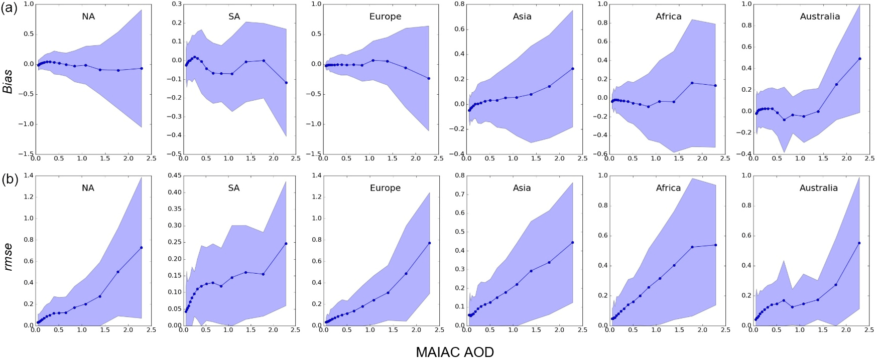
Figure 8 Bias (a) and RMSE (b) of MAIAC AOD for different world regions as a function of retrieved AOD. NA and SA stand for North and South America.

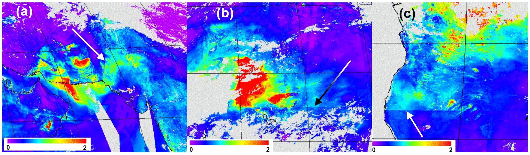
Figure 9 Illustration of MAIAC AOD contrast on the boundary of aerosol models (see Fig. 4) caused mainly by the difference in aerosol absorption between the models: (a) transition 8–2 (day 82, 2010), (b) transition 7–6 (day 113, 2010) and (c) transition 7–2 (day 237, 2010).

The global scatterplot of Fig. 7 shows that 66 % of retrievals (grey area) agree with AERONET within $\pm \mathrm{0.05}\pm \mathrm{0.1}$ AOD, which improves over the standard accuracy assessment of 15 % from the DT algorithm over land (e.g., Levy et al., 2013). While the global assessment may serve as a useful indicator of accuracy, the true performance of any algorithm is inherently regional and local, as shown by R, RMSE and bias statistics for each AERONET site. To generalize these assessments into regional prognostic error models, we computed RMSE and bias binned to retrieved AOD for different world regions. These results are summarized in Fig. 8, where the line shows the mean and the shaded area represents ± 1 standard deviation. Our analysis and results of independent studies (e.g., Superczynski et al., 2017; Mhawish et al., 2018) show that MAIAC AOD has little dependency on view geometry. Although MAIAC accuracy somewhat decreases over bright surfaces, here the regional analysis was done for all AERONET sites together. Figure 8 shows that the linear model for both mean and standard deviation can serve as a reasonable proxy for both RMSE and bias; for instance

$$\begin{array}{}\text{(18)}& \mathrm{RMSE}=a+b\times \mathrm{AOD}\pm (\mathit{\alpha }+\mathit{\beta }\times \mathrm{AOD})..\end{array}$$

The regional linear regression model parameters are given in Table 5. A more detailed MAIAC AOD error analysis, as in Sayer et al. (2013), will be given separately.

10.6 Known issues and limitations

Below is a list of currently known issues and limitations of algorithm MAIAC:

1. The maximum value of LUT AOD_0.47 is 4.0, which limits characterization of strong aerosol emissions.

2. MAIAC LUTs are built assuming pseudospherical correction in single scattering, which has a reduced accuracy for high sun/view zenith angles. A reduced MAIAC performance is expected at solar zenith angles $>\mathrm{70}{}^{\circ }$.

3. MAIAC may be missing bright salt pans in several world deserts. In such cases, it generates a persistently high AOD resulting in missing surface retrievals.

4. Geographic AOD boundaries may sometimes be observed on borders of the regional aerosol models when they have a significant difference in absorption. While this is not an issue over most of the globe, three transition zones may stand out during the biomass-burning seasons (see Fig. 4): the northwest boundary between India (model 8) and central Asia (model 2), and two transitions from central Africa to Sahel–Sahara (models 7–6) and to southern Africa (models 7–2). Figure 9 shows one the worst-case examples for each transition zone when at high AOD the contrast across the model boundary can be as high as 40–50 % of the mean value, while it is not noticeable for most of the year when AOD is moderate to low.

5. Because of inherent uncertainties of gridding on the coastline, the area of ±1–3 pixels from the coastline may contain frequent artifacts in cloud mask (usually overdetection), AOD (higher values) and surface BRF. Users should exercise caution near the coastline as indicated by QA.QA_AOD (value 1010).

6. AC over detected snow: as MAIAC does not retrieve AOD over snow, it assumes a low climatology AOD is 0.05 globally and 0.02 at high elevations (H>4.2 km). Over north-central China, which is often heavily polluted and where low-AOD assumption can lead to a significant bias, we use AOD averaged over a mesoscale area of 150 km using reliable AOD retrievals over snow-free pixels. Such an approach does improve the quality of AC compared to low-AOD assumption as judged by the reduced boundaries and diminished color artifacts, but it does not account for the aerosol variability inside a 150 km area, which may be significant.

7. The ice mask is currently unreliable.

8. A particular type of cloud (moderately thin and homogeneous cumulus) is consistently missed over water generating high AOD.

9. MAIAC uses a specialized “bay” mask for aerosol retrievals over coastal waters with high sediments. The current bay mask misses several these areas where AOD retrievals often show a high bias.

10. Since 2014, when MODIS Terra/Aqua calibration was consistently updated (Lyapustin et al., 2014b), the continued calibration degradation of MODIS Terra in MAIAC AOD increasingly appears via striping and a positive bias on the left-hand side of the MODIS scan, mostly over bright surfaces. The MODIS calibration was recently updated. It will be implemented in MODIS Collection 6.1 Land Discipline reprocessing (which includes MAIAC), scheduled for the second half of 2018. We expect a significant reduction of mentioned errors in MAIAC C6.1 AOD.

11 Conclusions

This paper presented the C6 MAIAC algorithm used in the ongoing MODIS Collection 6 processing. MAIAC cloud detection, aerosol retrieval and atmospheric correction over land were described in detail. Being the first publication of the official new MODIS product MCD19, this paper also provided the technical specification of MCD19 output files along with the brief quality assurance discussion and recommendations for use. Other MAIAC components related to detection and processing of snow, retrievals over water and smoke plume height retrieval will be described elsewhere.

The paper also presented a brief analysis of near-global MAIAC AOD validation against AERONET measurements along with error analysis. These results serve to complement the growing body of the air quality and land community studies of MAIAC data quality and its comparison to the standard MODIS products.