the Creative Commons Attribution 4.0 License.
the Creative Commons Attribution 4.0 License.
 | 27 Nov 2018
Comparison of methods to derive radial wind speed from a continuous-wave coherent lidar Doppler spectrum
Jakob Mann
Continuous-wave (cw) lidar systems offer the possibility to remotely sense wind speed but are also affected by differences in their measurement process compared to more traditional anemometry like cup or sonic anemometers. Their large measurement volume leads to an attenuation of turbulence. In this paper we study how different methods to derive the radial wind speed from a lidar Doppler spectrum can mitigate turbulence attenuation. The centroid, median and maximum methods are compared by estimating transfer functions and calculating root mean squared errors (RMSEs) between a lidar and a sonic anemometer. Numerical simulations and experimental results both indicate that the median method performed best in terms of RMSE and also had slight improvements over the centroid method in terms of volume averaging reduction. The maximum, even though it uses the least amount of information from the Doppler spectrum, performs best at mitigating the volume averaging effect. However, this benefit comes at the cost of increased signal noise due to discretisation of the maximum method. Thus, when the aim is to mitigate the effect of turbulence attenuation and obtain wind speed time series with low noise, from the results of this study we recommend using the median method. If the goal is to measure average wind speeds, all three methods perform equally well.
- Article
(2003 KB) - Full-text XML
- BibTeX
- EndNote


Remote sensing is an attractive alternative to traditional in situ measurements of wind speed. For wind turbines, light detection and ranging (lidar) devices can replace the installation of large meteorological masts hosting cup or sonic anemometers in order to meet the constantly increasing measurement height requirements. This flexibility led to a large variety of applications of lidars spanning from lidar-assisted yaw and pitch control (Schlipf, 2015) to site assessment (Sanz Rodrigo et al., 2013) and power curve validation (Borraccino et al., 2017). However, one has to keep in mind that there is one important principal difference between measurements from a lidar device and sonic or cup anemometers, namely the averaging over a rather large measurement volume.
Lidars can be operated in two different modes: laser light can either be emitted in continuous-wave (cw) or pulsed form. For a cw lidar, a laser beam is focused on the desired point in space and measures the backscattered light. The radial speed of the aerosols can be estimated from the induced Doppler shift of the backscattered light. However, there is an ambiguity in the definition of the dominant frequency of the Doppler spectrum. In early systems, simply the maximum value of the power spectral density (PSD) was used. But since this gives integer multiples of the frequency step (which depends on the fast Fourier transform set-up) it has the disadvantage of returning a noisy signal. Thus, nowadays most commercial cw lidar systems use the centroid of the PSD above a certain noise level (Harris et al., 2006), while in research instruments (e.g. short-range WindScanner) the median method is implemented (Angelou et al., 2012).
On the other hand, pulsed lidars emit a light pulse of finite length. This allows the atmosphere to be probed at several positions along the laser beam based on the current location of the light pulse as it propagates. For pulsed lidars significantly more investigations have been done on how to determine the radial speed from a Doppler spectrum. For example, Frehlich (2013) presents an investigation on the maximum likelihood (ML) algorithm and minimum mean squared error method. Both estimators had similar performance and the latter was chosen because of computational efficiency. In addition, Dolfi-Bouteyre et al. (2016) examined two simple methods (maximum and centroid), the previously mentioned ML approach, polynomial fitting and an adaptive filter method. The polynomial fitting method was found to perform best in laminar flow but it is suggested that in more complex flow, advanced estimators are needed. However, for a cw lidar these more complex methods are unavailable because they rely on an underlying model for the shape of the Doppler spectrum. According to the current knowledge of the authors no such model exists for cw lidars.
One of the measurement differences of a lidar compared to cup or sonic anemometers is its large probe volume, which leads to turbulent fluctuation attenuation. While the effect of the probe volume on turbulence attenuation can be modelled by theory for the centroid method, no theories exist for the median or maximum methods. Several studies aimed at validating the theory for the centroid method by comparing the spectral transfer function between a lidar and sonic anemometer, i.e. the ratio between the power density spectra of lidar and sonic measurements. An early study by Lawrence et al. (1972) compared a cw carbon dioxide (CO2) lidar to a cup anemometer around 10 m above the ground. Due to the short focus distance (approximately 30 m), the Rayleigh length was less than 0.5 m and analysis of the PSD showed no effect of the lidar's volume averaging. Another cw CO2 lidar at focus distances up to 200 m close to the ground was used in Banakh and Smalikho (1999). High-frequency fluctuation attenuation due to volume averaging was observed. A power spectral analysis showed significant deviations between the lidar and sonic power spectrum, starting at 0.4 Hz and becoming more severe at increasing frequencies. The experimental results support the theory developed in the paper.
A cw lidar focused close to a sonic anemometer mounted 78 m above ground was used in Sjöholm et al. (2009). Data gathered at 20 Hz were used to investigate the spatial averaging, and good agreement between theory and experiment was found. However, during periods with low-level clouds the measurements were affected negatively. The same objective was followed in Angelou et al. (2012), in which the transfer function of a tower-mounted horizontally staring lidar was determined against a mast-mounted sonic anemometer allowing for horizontal measurements. The study was limited to when the lidar beam was aligned with the wind direction, and during these periods the spatial averaging effect from measurements agreed perfectly with the theory for the centroid method attenuation. Further, this study presented a method to reduce the influence of noise at high frequencies by estimating the spectral transfer function using the cross-spectrum between lidar and sonic measurements and the auto-spectrum of the sonic anemometer.
Two studies investigated the spatial averaging of a long-range pulsed lidar compared to mast-mounted sonic anemometers (Fuertes et al., 2014; Mann et al., 2009). Both studies showed the feasibility of measuring 3-D wind vectors by synchronised lidars focused at one point in space. It was also shown that the attenuation from spatial averaging can be predicted by the theory for pulsed lidar systems, which is presented in the two studies.
A slightly different approach was followed in Peña et al. (2017). In this study a cw nacelle lidar and a pulsed nacelle lidar were compared against both a cup and sonic anemometer. Turbulence statistics was calculated by fitting a spectral tensor model including a lidar volume averaging model to the sonic measurements and an average Doppler spectrum method, which was also used in Branlard et al. (2013). The first method enabled the retrieval of filtered turbulence statistics, while the second yielded measures not affected by spatial averaging. These results reiterated that predictions of the spatial averaging effect are consistent with theory.
A machine-learning approach to produce unfiltered wind speed variances from pulsed lidar signals was used in Newman and Clifton (2017). Besides a model for spatial averaging, the algorithm also includes automatic noise removal. Comparisons to sonic anemometers showed improvements when using the algorithm under all stability classes, but the results are highly dependent on the input variables and the training sets.
From the studies mentioned above it can be seen that the effect of the lidar's spatial averaging can be predicted theoretically, which has also been confirmed experimentally. In contrast to pulsed lidars, little work has been done on the effect of how the radial wind speed is calculated from a Doppler spectrum for cw lidars. Thus, the objective of this study is to investigate the influence of using different methods of determining the dominant frequency in a lidar Doppler spectrum (maximum, median, centroid) and its influence on the volume-averaging effect of lidar measurements. This is important because the lidar's probe volume has an attenuating effect on the measurement of turbulent fluctuations. As a consequence, estimates of wind speed variances will be biased if the lidar is used for site characterisation. Also for lidar-assisted control integration an accurate measurement of the turbulent fluctuations is important. Since no theory has been formulated for the median and maximum method yet, the study was motivated by initial numerical simulations that showed improved performance for these two methods compared to the centroid method. In this study the numerical simulations are extended and compared to data gathered during a field experiment.
Statistically, the fluctuating part of an incompressible, homogeneous wind field u(x) can be described by the spectral tensor Φij(k), where k is the wave number vector. To simulate synthetic wind fields, models for Φij(k) have been derived, e.g. von Karman (1948) or Mann (1998). This allows us, on the one hand, to directly calculate the statistical behaviour of a point measurement (i.e., from a sonic anemometer) and a volume measurement (i.e., from a lidar) in wave number space, and on the other hand, to generate a simulated box of turbulence. These boxes consist of wind velocity values at specified grid points that are frozen in space. They can be used to simulate the lidar measurement process and calculate Doppler spectra from which the radial wind speed can be derived. Both methods will be compared to the experimental findings.
2.1 Theory
A cw lidar measurement can be modelled by the convolution of the projected radial component n⋅u and a weighting function (Sonnenschein and Horrigan, 1971):
where zR is the so-called Rayleigh length that characterises the probe volume, s is the distance from the focus point along the beam, n is the beam unit vector and r is the focus position. The Rayleigh length can vary from a few centimetres at small focus distances to tens of metres at very large focus distances and varies with the focus distance squared, i.e. (Hu, 2016).
Equation (1) assumes the definition of the centroid of the Doppler spectrum; in the following we will refer to it as cen. Another method of determining the dominant frequency in a Doppler spectrum is by simply taking the frequency bin where the peak occurs (max) or by treating it as a probability density function (PDF) and taking the median value (med). The estimated radial wind speed using these three methods will be compared to the laser-line-projected sonic wind velocity . This will be done for the numerical simulations and the experiment.
To evaluate how well lidar and sonic measurements correlate in the wave number domain, an estimation of the transfer function between the two signals is used:
where χr, s(k1) refers to the cross-spectrum between the lidar and sonic signal and Fs(k1) refers to the auto-spectrum of the sonic signal. The closer G(k1) is to unity, the smaller the effect of volume averaging of the lidar is. We prefer to use the transfer function defined in Eq. (2) to the more traditional because the auto-spectrum Fr(k1) may be affected by noise whereas the cross-spectrum χr, s(k1) is not (Angelou et al., 2012), assuming the sonic measurements contain considerably less noise than the lidar measurements.
When using , Eq. (1) can be expressed in wave number space by
where ℱ[.] refers to the Fourier transformation. The integration in Eq. (3) can only be solved analytically for simple forms of Φij(k). For the line-of-sight projected sonic measurement vs, which can be approximated by a point measurement due to the small volume measurement, the exponential term in Eq. (3) drops out and we are left with
The cross-spectrum between the lidar and sonic measurements can then be written as
It should be noted that is only true when the lidar beam is aligned with the mean wind direction. In misaligned cases holds (Kristensen and Jensen, 1979). Thus, for misaligned cases we do not expect the transfer function to tend towards unity for small wave numbers.
Another measure used to evaluate the performance of the different methods is the root mean squared error (RMSE):
where method refers to either centroid, median or maximum and the overbar indicates averaging in time. In contrast to the transfer function estimate mentioned previously, for this measure, noise in lidar measurements will affect the performance and gives an indication of the difference between lidar and sonic measurements in the time domain.
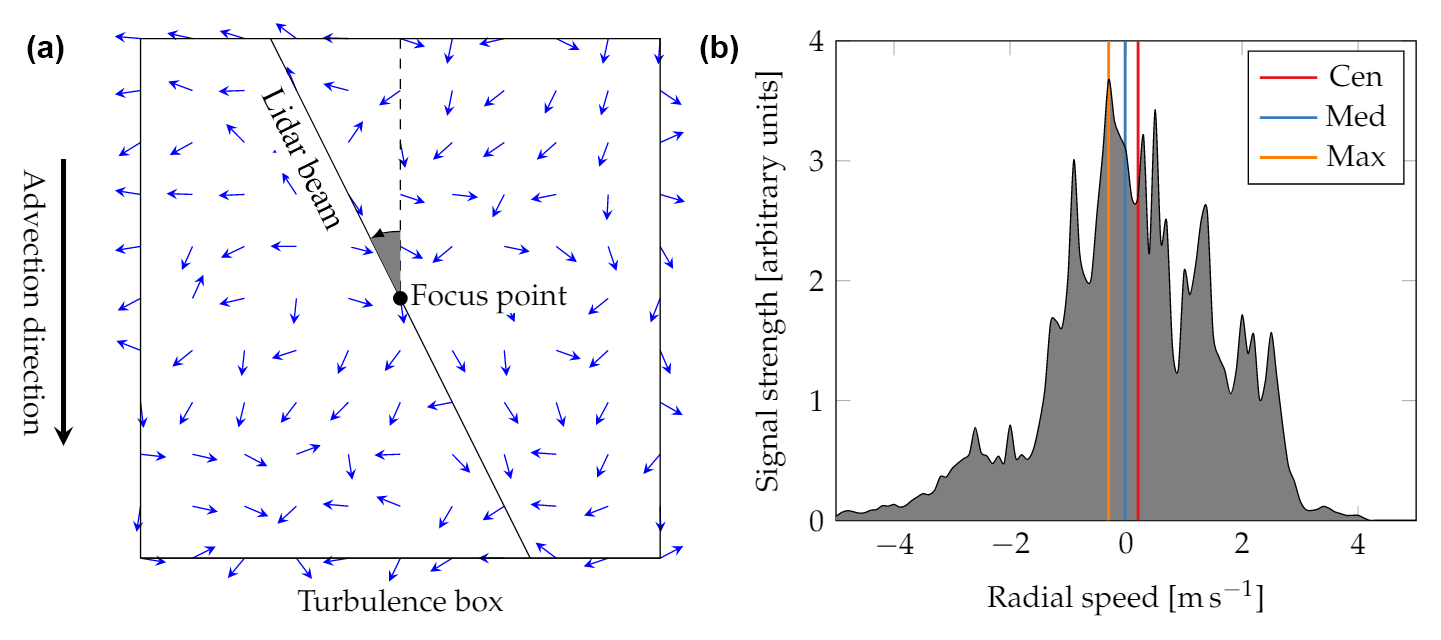
Figure 1(a) Illustration of the lidar simulation set-up. (b) Example of an instantaneous Doppler spectrum, in which the radial wind speed has been determined by the three different methods.
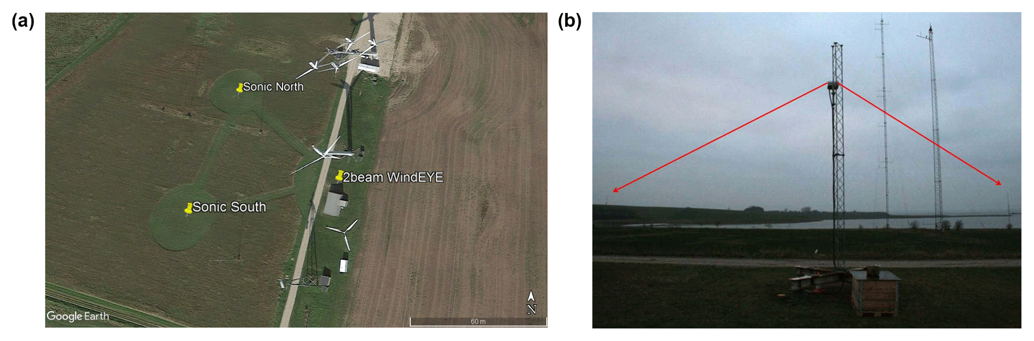
Figure 2(a): Google Earth screenshot of the site set-up. (b) Photo depicting the lidar mounted on the mast looking at the two sonic anemometers, from Dellwik et al. (2015).
2.2 Numerical simulations
Numerical simulations illustrate results in an environment where no noise is present. The methodology used to perform these simulations was developed in Mann (1998). First it is described how a Doppler spectrum is obtained from a simulated wind time series. We narrowed our investigation to the (horizontal) 2-D case in which the cw lidar measures horizontally only. We furthermore assumed Taylor's frozen turbulence hypothesis:
where U is the mean wind speed, so the wind field at any given time can be obtained by translating the wind field at t=0. We did not consider any sources of noise. In this case the Doppler spectrum S(v, t) can be written as
where δ is the Dirac delta function. Notice that Eq. (8) is a convolution of the weighting function φ and the delta function . If φ was disregarded, Eq. (8) could be viewed as a histogram of wind velocities. The discretisation of the histogram is chosen to match the typical velocity bin resolution of a lidar system, which in this simulation case was 0.1 ms−1 bin−1. When φ is included, the wind velocities are weighted, such that the velocities around the focus point count most. Due to the finite length of the simulated turbulent boxes, the integration in Eq. (8) needs to be truncated. Here we chose a distance of M=12zR along the beam after which the truncation is applied, where the Lorentzian weighting function has a value of (or 0.69 % relative to the maximum value at the focus point):
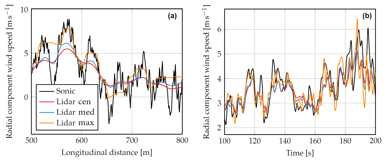
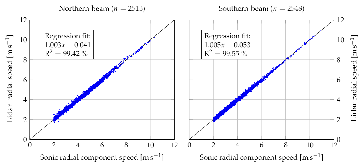
Figure 410 min average sonic radial component speed versus lidar wind speed. The lidar wind speed has been calculated using the centroid method.
To generate the wind time series we assumed for simplicity that the turbulent fluctuations in the direction of the mean wind can be described by the model by Mann (1994)1. A turbulent wind box was created with a horizontal 2-D wind vector at each grid point. The dimensions of the box are 4096×4096 grid points with a separation of 0.732 m. A total of 20 turbulent boxes with different initial turbulence seeds have been simulated, resulting in 20 different realisations of the turbulent field. Note that here we only simulate the fluctuating part, and the mean wind speed is zero. An illustration of the simulation set-up and an example of a simulated Doppler spectrum including the radial wind speed estimates using the three different methods is shown in Fig. 1.
2.3 Experimental set-up
In this section the experiment conducted at Risø campus with a lidar system by Windar Photonics A/S will be presented. The WindEYE is a commercial Doppler wind lidar that uses an all-semiconductor laser source with a wavelength of 1553 nm; see Hu (2016). Because the purpose of the product is wind direction measurement, it can focus in two positions by deflecting the beam through two different lenses. The switching occurs every half second, which means that the lidar focuses on one position for 0.5 s and then a liquid crystal will bend the beam towards the second focus point for another 0.5 s. Usually the device is mounted on the nacelle of wind turbines, but for this experiment it was installed on a tower to be able to focus on the location of two sonic anemometers around 10 m above the ground; see Fig. 2. The lidar beams are aligned horizontally to measure horizontal components only. The focus distance is 90 m and the Rayleigh length zR is 14.5 m. The angle between the two beams is 60∘, but since the beams are compared individually it is of no importance here.
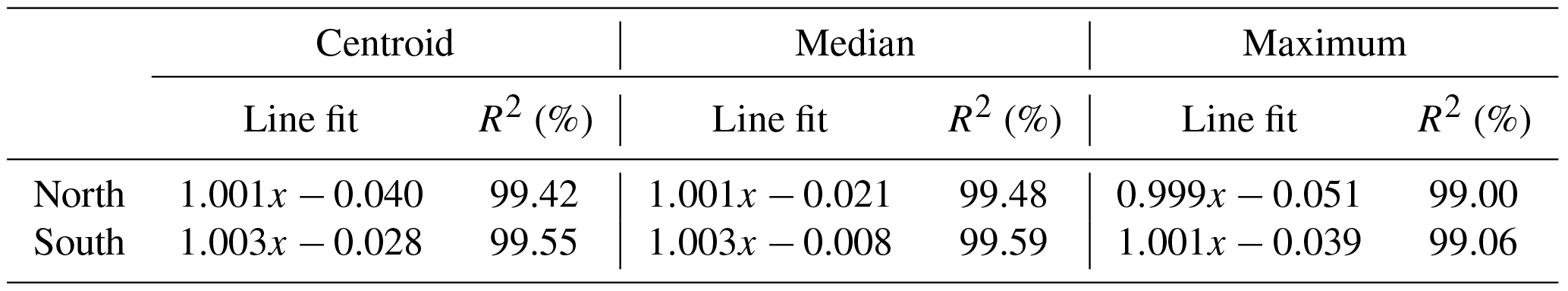
Table 1Parameters of the line fit to the 10 min correlation between the sonic radial component and lidar.
The sonic anemometers are two USA-1 anemometers by Metek GmbH, which were mounted on a tower at the exact position of the focus points. The focus distances have been verified experimentally in an optical laboratory, and the alignment of the lidar to the sonic anemometers was checked using an infrared sensor card; see Dellwik et al. (2015). The laser beams pass approximately 1 m above the sonic devices.
The sonic anemometers were sampled at 35 Hz and have a transducer distance of 0.175 m implying that the device retrievals approximate a point measurement compared to the averaging volume of the lidar. For all measurements the standard 2-D flow correction has been removed and instead a 3-D correction was used (Bechmann et al., 2009). Due to the inherent switch mechanism of the WindEYE lidar the data had to be combined to a rather low sampling frequency of 1 Hz. The experiment extended from 9 January to 23 March 2014 but due to synchronisation problems only the periods in February and March could be used.
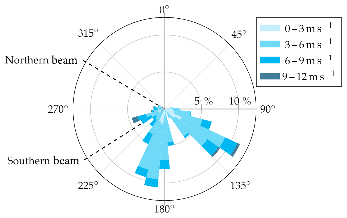
Figure 5Wind rose derived from 10 min averages of sonic anemometer wind speed and direction of the 2-month-long experiment. The beam directions are indicated as dashed lines.
In this section we first present an example of the numerical simulation and experimental results and then we will compare both to the analytical results. An example of the numerical simulation and the experiments can be found in Fig. 3.
3.1 Experimental results
At first the 10 min averages of the lidar measured wind speed component vr and the 3-D sonic wind vector projected on the line of sight, n⋅u, have been compared. A filter has been applied for radial components less than 2 ms−1 because it is not possible to accurately determine vr below that value for a homodyne lidar system. The comparison can be seen in Fig. 4. For both beams a very good comparison can be observed; the line fits yield slopes of unity and an R2 of almost 100 %. The line fits for the other methods can be found in Table 1. The difference between the methods is negligible. An example of a time series result can be found in Fig. 3.
The wind rose derived from the two sonic anemometers is shown in Fig. 5. Mean wind speed and direction were calculated over 10 min periods and then the average of both anemometers was taken. Two main wind directions can be identified, of which one is aligned with the northern beam direction. Thus, more data were gathered for a misalignment of 0∘ for the northern beam compared to the southern beam.
For wind lidar systems using a homodyne detection method, there is an ambiguity in the wind direction (whether the wind blows towards or away from the lidar). Further the limitation to the line-of-sight component of the wind vector leads to an ambiguity in the misalignment (whether the wind direction is misaligned towards the left or right side of the beam). In all these cases the radial wind speed measurements will be the same. For example, a case of a wind direction misaligned by 10∘ is equivalent to a misalignment of 170, 190 and 350∘. Thus, it is possible to reduce the full 360∘ to one quadrant ranging from 0 to 90∘. In the following analysis the data have been binned into 10∘ sectors ranging from 0 to 90∘.
To create numerical simulations as close as possible to the experimental conditions, the Mann spectral tensor has been fitted, following the procedure in Mann (1994), to the u and v spectra obtained from sonic measurements, where the mean wind speed was above 6 ms−1. The tensor model has three parameters: αϵ2∕3, where ϵ is the rate of viscous dissipation of turbulent kinetic energy and α is the spectral Kolmogorov constant; L, which is a length scale; and Γ, which is an anisotropy parameter. For details, see Mann (1994). This has been done sector-wise for sectors of 10∘ for each beam, and the results can be seen in Table 2.
In order to reduce the computational effort, we have taken the average value of each parameter over all sectors and both beams and found the following parameter: m4∕3s−2, L=22.3 m, Γ=2.26. These parameters have been used to perform the numerical simulations mentioned in Sect. 2.2.
Table 2Sector-wise fitted parameters of the Mann model for each beam to data obtained from sonic measurements at 10 m over 2 months.

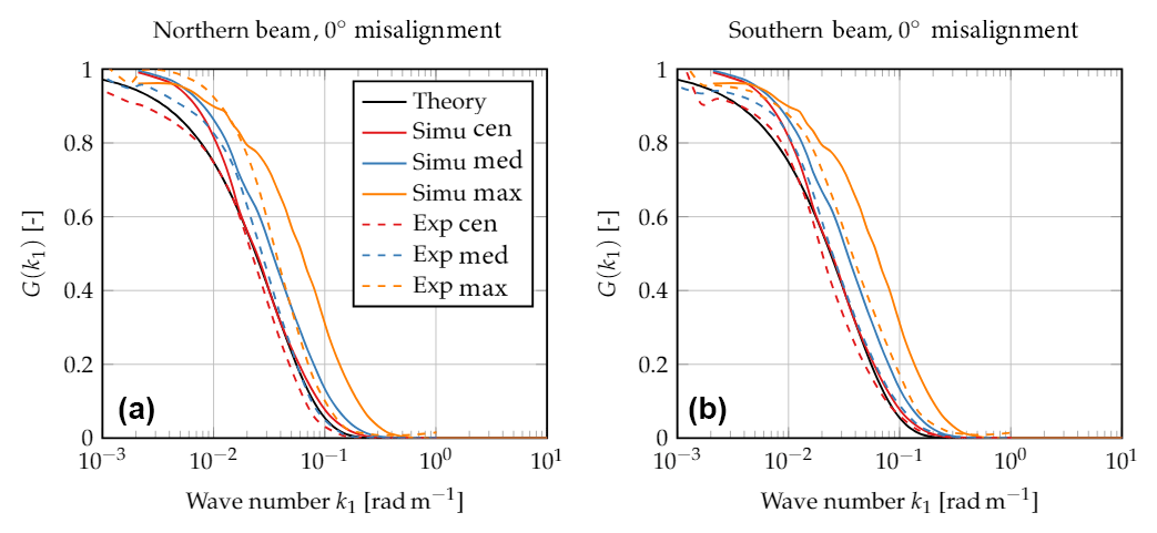
Figure 6Transfer function G(k1) for aligned beams for the northern beam data (a) and southern beam data (b) using 20 simulations and 2 months of experimental data at a sampling rate of 1 Hz.
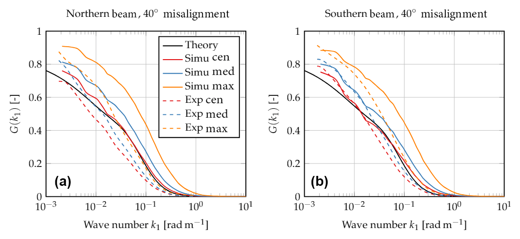
Figure 7Transfer function G(k1) for misaligned beams for the northern beam data (a) and southern beam data (b) using 20 simulations and 2 months of experimental data at a sampling rate of 1 Hz.
3.2 Theoretical, numerical and experimental results
In this section we will present the combination of experimental and simulation results together with the numerical integration of Eq. (2) (using Eqs. 3–5). In the following plots theoretical results are represented by a solid black line, simulation results (Simu) by coloured solid lines and experimental results (Exp) by coloured dashed lines. The different colours stand for the three methods to derive the radial speed from the Doppler spectrum: centroid (cen), median (med) and maximum (max).
First, we present the simplest case when the lidar beam is aligned with the wind direction. In this case Eq. (2) can be solved analytically because the exponential in Eqs. (3) and (5) does not depend on either k2 or k3 and can be moved outside the integral. This results in
Note that in Eq. (10) the radial speed is defined by the centroid method. For the aligned case the transfer function only depends on zR and not on the turbulence model parameters.
The results for the aligned case are shown in Fig. 6, where Eq. (10) is shown as the black solid line. It can be seen that both red lines (solid and dashed) agree well with the theoretical results. Some significant deviations can be observed for the simulation results at small wave numbers, which can be explained by the truncation of the Doppler spectrum in Eq. (9).
It can also be seen that the transfer functions when using the median or maximum method lie above the results for the centroid method. This indicates that the turbulence attenuation is less severe for these two methods compared to the centroid method. Thus, fluctuations which have been measured by the sonic and are attenuated when using the centroid method due to volume averaging can indeed be sensed when using the median and maximum method. The improved performance is stronger for the numerical simulation due to the absence of noise. The median method seems to perform slightly better than the centroid method, and the maximum method has an even bigger improvement.
As an example for a misaligned case, we will now focus on a misalignment of 40∘; see Fig. 7. The transfer functions for the remaining misalignments can be found in the Appendix. For a misalignment of 40∘, Eq. (10) is not valid anymore. However, Eq. (2) can be integrated numerically. It is shown again as the solid black line. Again we can see that the simulation results using the centroid method matches the theoretical results well for large wave numbers, but there are deviations at low wave numbers. Similar to the aligned case, it can be observed that the transfer functions for the median and maximum method lie above that of the centroid method. Again, this implies that turbulent fluctuations that were not measured using the centroid method can be sensed using the median and maximum method. The maximum method again shows the best performance.
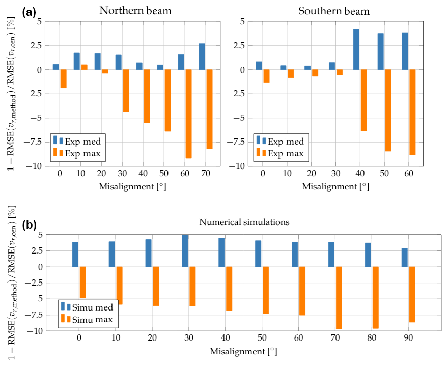
Figure 8RMSE value for the median and maximum method normalised by RMSE(vr, cen) for the experimental results (a) and the numerical simulations (b) using 20 simulations and 2 months of experimental data at a sampling rate of 1 Hz.
Examples of these improvements can also be identified in the time domain when looking at Fig. 3. For the numerical simulations (panel a) the improved fluctuation measurements using the maximum method are very clear, while the median method is also able to slightly enhance the measurements compared to the centroid method, which performs worst. A similar tendency is also observed from the experiment (panel b). Just before 120 s we can note a very good agreement between sonic and maximum-method vr, whereas the other two methods are not able to detect this fluctuation. In other periods the observed improvement is very small.
Next we consider the RMSE results. Since it was seen previously that both the median and maximum method outperformed the centroid method, the RMSE of the two methods normalised by the RMSE of the centroid is compared now:
where method is either the median or the maximum method. Thus positive numbers indicate better performance compared to the centroid method and vice versa.
The results can be seen in Fig. 8 and show that the median method consistently outperforms the centroid method. Improvements of up to 4 % from the experimental data was observed, while the simulations showed performance increases between 3 % and 5 %. In contrast, the maximum method has persistent disadvantages compared to the centroid method. The shortcoming increases with increasing misalignment and reaches values of approximately −9 % for the experiments and close to −10 % for the numerical simulations. This indicates that the improved performance of the maximum method in reducing the effect of spatial averaging has the consequence that more signal noise is introduced. This is the result of selecting the maximum of the Doppler spectrum since the maximum position can vary depending on the frequency bin width and Doppler spectrum noise. The other two methods are more robust against noise contamination.
In this study we compared a cw wind lidar to sonic measurements, where the sonic anemometers are mounted exactly at the focus positions of the lidar system. The lidar measurements are affected by their large probe volume, which leads to an attenuation of turbulence. The objective of the paper was to study how different methods of determining the dominant frequency in a Doppler spectrum affect wind speed measurements by a cw lidar. We used an estimation of the transfer function to evaluate the lidar's attenuation of turbulent fluctuations and the RMSE to give a metric to the general performance of the methods. Theoretical analysis, numerical simulation and data from a 2-month-long experiment have been used, and three different methods for deriving the radial speed were applied: the centroid, median and maximum method.
The analysis was able to show that the simulations, as well as the experiments, agree well with the theoretical results for the centroid method. Further, the median and maximum methods performed better both in simulations and experiments compared to the centroid method in reducing the effect of spatial averaging. Interestingly the maximum method had the highest reduction of the effect of spatial averaging. However, it also showed the highest RMSE values out of all methods due to the discretisation of picking the maximum value of the Doppler spectrum. Thus, from this study we recommend, if one's aim is to mitigate the effect of turbulence attenuation by the lidar and retrieve time series with low noise levels, using the median method as it shows slight improvements of reducing the volume effect compared to the centroid method and has the best RMSE performance. When comparing 10 min averages all methods performed equally well.
The method of using average Doppler spectra (typically 10 or 30 min averages) has also been studied to derive turbulence statistics (Branlard et al., 2013). However, using this approach, only statistics can be derived, namely the wind speed PDF and its statistical moments. What is presented here shows how carefully choosing the method of radial speed retrieval from a Doppler spectrum can partly alleviate the inherent volume averaging effect of lidar systems to provide time series information.
It should be noted that these conclusions only apply to cw lidars and not to pulsed systems as the method of deriving radial velocities is different for the latter.
The computer code to generate synthetic turbulence fields can be found at http://www.wasp.dk/weng#details__iec-turbulence-simulator (WAsP Engineering, 2018).

Figure A1Transfer function G(k1) for the remaining misalignment directions.
DPH performed the research work and prepared the manuscript. JM conceived the research plan and supervised the research work and the manuscript preparation.
The work of Dominique P. Held was partly funded by Windar Photonics A/S through an industrial PhD stipend (project number: 5016-00182).
This study was supported by Innovationsfonden Danmark in the form of an
industrial PhD stipend (project number: 5016-00182). The authors want to
thank Ebba Dellwik and Antoine Larvol for their support with the sonic
anemometer and lidar data.
Edited by: Ad
Stoffelen
Reviewed by: two anonymous referees
Angelou, N., Mann, J., Sjöholm, M., and Courtney, M. S.: Direct measurement of the spectral transfer function of a laser based anemometer, Rev. Sci. Instrum., 83, 033111, 2012. a, b, c
Banakh, V. A. and Smalikho, I. N.: Measurements of turbulent energy dissipation rate with a CW Doppler lidar in the atmospheric boundary layer, J. Atmos. Ocean. Technol., 16, 1044–1061, 1999. a
Bechmann, A., Berg, J., Courtney, M. S., Jørgensen, H. E., Mann, J., and Sørensen, N. N.: The Bolund Experiment: Overview and Background, Tech. rep., Risø-R-1658(EN), DTU, available at: http://orbit.dtu.dk/files/4321515/ris-r-1658.pdf (last access: 22 November 2018), 2009. a
Borraccino, A., Courtney, M. S., and Wagner, R.: Remotely measuring the wind using turbine-mounted lidars: Application to power performance testing, PhD thesis, Technical University of Denmark, Lyngby, Denmark, 2017. a
Branlard, E., Pedersen, A. T., Mann, J., Angelou, N., Fischer, A., Mikkelsen, T., Harris, M., Slinger, C., and Montes, B. F.: Retrieving wind statistics from average spectrum of continuous-wave lidar, Atmos. Meas. Tech., 6, 1673–1683, https://doi.org/10.5194/amt-6-1673-2013, 2013. a, b
Dellwik, E., Sjöholm, M., and Mann, J.: An evaluation of the WindEye wind lidar, Tech. rep., Technical University of Denmark, Lyngby, Denmark, 2015. a, b
Dolfi-Bouteyre, A., Canat, G., Lombard, L., Valla, M., Durécu, A., and Besson, C.: Long-range wind monitoring in real time with optimized coherent lidar, Opt. Eng., 56, 031217, 2016. a
Frehlich, R.: Scanning doppler lidar for input into short-term wind power forecasts, J. Atmos. Ocean. Technol., 30, 230–244, 2013. a
Fuertes, F. C., Iungo, G. V., and Porté-Agel, F.: 3D turbulence measurements using three synchronous wind lidars: Validation against sonic anemometry, J. Atmos. Ocean. Technol., 31, 1549–1556, 2014. a
Harris, M., Hand, M., and Wright, A. D.: Lidar for turbine control, Tech. rep., NREL/TP-500-39154, https://doi.org/10.2172/881478, 2006. a
Hu, Q.: Semiconductor Laser Wind Lidar for Turbine Control, PhD thesis, Technical University of Denmark, Lyngby, Denmark, 2016. a, b
Kristensen, L. and Jensen, N. O.: Lateral coherence in isotropic turbulence and in the natural wind, Boundary-Layer Meteorol., 17, 353–373, 1979. a
Lawrence, T. R., Wilson, D. J., Craven, C. E., Jones, I. P., Huffaker, R. M., and Thomson, J. A. L.: A Laser Velocimeter for Remote Wind Sensing, Rev. Sci. Instrum., 43, 512–518, 1972. a
Mann, J.: The spatial structure of neutral atmospheric surface-layer turbulence, J. Fluid Mech., 273, 141–168, 1994. a, b, c
Mann, J.: Wind field simulation, Probabilistic Eng. Mech., 13, 269–282, 1998. a, b
Mann, J., Cariou, J. P., Courtney, M. S., Parmentier, R., Mikkelsen, T., Wagner, R., Lindelöw, P., Sjöholm, M., and Enevoldsen, K.: Comparison of 3D turbulence measurements using three staring wind lidars and a sonic anemometer, Meteorol. Z., 18, 135–140, 2009. a
Newman, J. F. and Clifton, A.: An error reduction algorithm to improve lidar turbulence estimates for wind energy, Wind Energ. Sci., 2, 77–95, 2017. a
Peña, A., Mann, J., and Dimitrov, N.: Turbulence characterization from a forward-looking nacelle lidar, Wind Energy Sci., 2, 133–152, 2017. a
Sanz Rodrigo, J., Borbón Guillén, F., Gómez Arranz, P., Courtney, M. S., Wagner, R., and Dupont, E.: Multi-site testing and evaluation of remote sensing instruments for wind energy applications, Renew. Energy, 53, 200–210, 2013. a
Schlipf, D.: Lidar-Assisted Control Concepts for Wind Turbines, PhD thesis, University of Stuttgart, 2015. a
Sjöholm, M., Mikkelsen, T., Mann, J., Enevoldsen, K., and Courtney, M. S.: Spatial averaging-effects on turbulence measured by a continuous-wave coherent lidar, Meteorol. Z., 18, 281–287, 2009. a
Sonnenschein, C. M. and Horrigan, F. A.: Signal-to-Noise Relationships for Coaxial Systems that Heterodyne Backscatter from the Atmosphere., Appl. Opt., 10, 1600–1604, 1971. a
von Karman, T.: Progress in the Statistical Theory of Turbulence, P. Natl. Acad. Sci. USA, 34, 530–539, 1948. a
WAsP Engineering: IEC Turbulence Simulator, available at: http://www.wasp.dk/weng#details__iec-turbulence-simulator, last access: 22 November 2018.