Can turbulence within the field of view cause significant biases in radiative transfer modeling at the 183 GHz band?

The hypothesis whether turbulence within the passive microwave sounders field of view can cause significant biases in radiative transfer modeling at the 183 GHz water vapor absorption band is tested. A novel method to calculate the effects of turbulence in radiative transfer modeling is presented. It is shown that the turbulent nature of water vapor in the atmosphere can be a critical component of radiative transfer modeling in this band. Radiative transfer simulations are performed comparing a uniform field with a turbulent one. These comparisons show frequency dependent biases which can be up to several kelvin in brightness temperature. These biases can match experimentally observed biases, such as the ones reported in Brogniez et al. (2016). Our simulations show that those biases could be explained as an effect of high-intensity turbulence in the upper troposphere. These high turbulence phenomena are common in clear air turbulence, storm or cumulus cloud situations.

1 Introduction

Radiative transfer models (RTMs) are key tools in the microwave and infrared atmospheric remote sensing of the atmosphere. They are used to model the radiances at the top of the atmosphere as measured from satellites. The main inputs to the RTMs are atmospheric profiles of temperature, water vapor and trace gases, as well as surface properties, such as surface temperature and emissivity. The RTM simulate the absorption and emission of the molecular constituents of the atmosphere in a layer-by-layer approach. Their accuracy depends on the accuracy to which the spectral properties of the molecular absorption/emission lines are known, as well as the quality and vertical resolution of the vertical profiles of temperature, pressure and concentration of absorbing gases. By applying inversion techniques to these RTMs, such as Optimal Estimation (Rodgers, 2000), the physical parameters of the atmosphere can be obtained from radiances observed from satellites. These inversion techniques are commonly used in retrieval processes, where atmospheric properties are directly estimated from the measurements. They are also used in Numerical Weather Prediction (NWP) models, where measured radiances are assimilated as corrections to forecasts to form what are best estimates of the atmosphere, known as analyses. RTMs are, therefore, elements that bridge the gap between measured satellite radiances and atmospheric physical parameters such as profiles of temperature and water vapor concentration.

Although RTMs have achieved a high degree of accuracy, there is often, in practice, a systematic mismatch between what is observed and what is calculated from the RTMs. Their cause is varied and can range from an incorrect or incomplete implementation of the radiative transfer model setup, to uncalibrated instrumental effects or deviations in their nominal performance. These systematic mismatches are usually solved, in practice, by determining, for a particular satellite instrument, an offset or bias between measured and calculated radiances. This bias is then later corrected for retrievals and NWP assimilation systems. This practical fix is far from perfect, since deviations between systems are corrected with a simple bias or offset, when the reality can be more complex, depending on the underlying physical principles behind these systematic mismatches. For example, if a satellite system is deviating from its nominal behavior, ideally, the physical principles behind it should be sought for and corrected. If, on the other hand, radiative transfer is not modeled properly, the missing physical pieces should be put in place such that satellite measurements and RTM calculated radiances are consistent.

One of such mismatches occur in the 183 GHz water vapor absorption band, which has been noted by Clain et al. (2015) and Moradi et al. (2015). To discuss this effect, a “Joint workshop on uncertainties at 183 GHz” (Brogniez et al., 2015) was convened to discuss biases observed between measurements at 183 GHz and calculations using different RTMs plus either radiosondes or short range forecasts from NWP systems. The results were reflected in a paper published one year later (Brogniez et al., 2016). The values of the differences between observed and calculated brightness temperatures between the SAPHIR Megha-Tropiques instrument vs. Météo France NWP profiles plus the RTTOV v11 RTM are reproduced here as blue dots in Fig. 4. For further information and more results, with data from other instruments and other NWP models, please refer to Brogniez et al. (2016).

The potential causes behind these biases can be varied. Many plausible hypothesis could be formulated, such as poorly modeled gas absorption, effect of clouds, etc. In this paper we will discuss whether these significant detected biases can be caused by turbulence effects in the atmosphere. The rationale behind this hypothesis is based on the fact that radiative transfer is an extremely non-linear process. It is then possible that the average of the radiances at the top of the atmosphere, obtained from several neighboring different atmospheric columns, are not necessarily equal to the radiance computed from the average of all atmospheric columns. Which in turn, implies that radiances coming from a turbulent medium within the field of view of the instrument may be different from the radiances originating in a uniform medium.

Turbulence is a well known phenomena occurring in the atmosphere. Its spatial properties are commonly measured from the ground using in situ or remote sensing instruments. Turbulence in the troposphere is measured using sonic anemometers on meteorological towers (Champagne et al., 1977), hot wire anemometers suspended on tethered lifting systems (Frehlich et al., 2006), wind profiling radars (Hocking, 1985), passive microwave sounding (Kadygrov et al., 2003), Doppler wind lidar (see review from Sathe and Mann, 2013 and references therein), elastic backscatter lidar (e.g., Pal et al., 2010), ozone differential absorption lidar (Senff et al., 1996), water vapor differential absorption lidar (e.g., Senff et al., 1994; Kiemle et al., 1997; Wulfmeyer, 1999; Lenschow et al., 2000), and water vapor Raman lidar (e.g., Wulfmeyer et al., 2010; Turner et al., 2014; Behrendt et al., 2015). Individual sonde measurements have also proved to be a suitable instrument to measure turbulence (Thorpe, 1977; Wilson et al., 2011).

In the stratosphere, the measure of turbulence is tightly linked to the measure of gravity waves, since they share similar time and spatial scales. Detection of turbulence or gravity waves is usually made with remote sensing instruments. One of them is the satellite based microwave limb sounder (MLS; Waters et al., 2006) with which gravity waves can be detected (e.g., McLandress et al., 2000; Jiang et al., 2004). Passive microwave sounders on board of polar orbiting satellites have also been used to detect gravity waves (e.g., Eckermann and Wu, 2006). Airglow measurements can also be used to detect gravity waves, either using ground-based measurements (e.g., Sedlak et al., 2016) or space-borne ones (e.g., Yue et al., 2014). Infrared hyperspectral sounders such as AIRS and IASI have also proven to be useful for the measurement of gravity waves (Hoffmann et al., 2014).

The effect of turbulence in the modeling of the propagation of light in the atmosphere is taken into consideration in certain fields of astronomy and communication, where different effects of scintillation are studied. Studies of this sort are abundant in the literature (e.g., Leroy et al., 1979; Lencioni et al., 1981). Although high variability effects in the atmosphere are taken into account when looking for gravity waves in the stratosphere (e.g., Eckermann and Wu, 2006), they are often neglected in operational radiative transfer modeling for passive microwave sounders. The main reason for this is that operational radiative transfer models need to be fast and any saving in the already relatively heavy computation time is welcomed. Therefore, phenomena that do not, at first sight, seem to be needed are excluded. One such example is the effect in radiative transfer modeling of atmospheric turbulence within the field of view of microwave or infrared instruments. In this paper, an attempt to evaluate its significance in the radiative transfer modeling of the microwave 183 GHz band is shown. It will be shown that this effect can be quite important in some situations. The intensity of turbulence can vary several orders of magnitude within the troposphere. The typical values that will be used in this paper will be taken from Chen (1974), in particular, its Fig. 2. Typical values in the low troposphere are usually in the range between 1 and 10 cm² s⁻³. Close to the tropopause, values vary greatly spanning from 10⁻³ to 10⁴ cm² s⁻³ (Chen, 1974). The latter huge values occur in clear air turbulence, severe storm or cumulus cloud situations. It should be noted that in some particular cases, turbulence intensity could be outside of these limits and could well exceed the maximum values that are stated there.

In Sect. 2 a quantitative estimation of turbulence is made from measurements from dual sequential radiosondes. Section 3 shows how to calculate the effects of turbulence in radiative transfer modeling. In the discussion section, Sect. 4, its effect in the top of the atmosphere radiances is calculated and comparisons are made with the observed biases (Brogniez et al., 2016). In the conclusions section a summary of the results is made.

2 Turbulence from radiosondes

In this section, an estimation of the order of magnitude of atmospheric turbulent variables is performed. Parameters such as turbulent energy dissipation rates, turbulence length scales and turbulent atmospheric parameter variance are determined from sonde measurements. The main objective is to estimate the order of magnitude of these parameters, and, by the use of an RTM, an estimate of the order of magnitude of turbulent effects in microwave brightness temperature can be made.

The analysis of radiosonde data for its comparison with satellite measurements has shown that temperature and water vapor have a spatial behavior that is difficult to determine from just one radiosonde measurement (Calbet et al., 2017). More than one measurement is needed to resolve the small scale variability of the atmosphere, such as launching two consecutive sondes (Calbet et al., 2011, 2017). Another alternative is to make a spatial average of the measurements (Buehler et al., 2004) or to have a low spatial variability (Bobryshev et al., 2018) to have consistency between radiosonde and satellite measurements. The reason behind this is that spatial and temporal scales for water vapor are extremely small, as shown, for example, by Carbajal-Henken et al. (2015). This kind of behavior is typical of turbulent systems, such as the atmosphere.

Structure functions are tools that are often used in turbulence measurement, which are closely related to spatial auto-correlation functions. To effectively determine and quantify the turbulent nature of the atmosphere, the structure function of temperature and water vapor was determined. This was done with radiosonde data coming from the EUMETSAT MetOp campaigns which took place in 2007 and 2008 at Lindenberg and Sodankylä. In these campaigns, two consecutive radiosondes were launched from the same site with 50 min time difference. From now on, they will be referred here as sequential sondes. From Lindenberg and Sodankylä 266 and 359 sonde pairs were launched, respectively, making a total of 625 sonde pairs. The instrument payload analyzed here are the conventional RS92 radiosondes. For more details of this campaign and its instrumentation we refer the reader to Calbet et al. (2011). The data was later processed by GRUAN (Dirksen et al., 2014), which, among other advantages, greatly removes the humidity measurement dry biases usually present in RS92 measurements at the high troposphere (Miloshevich et al., 2009).

The computed structure functions for temperature and water vapor are shown in Fig. 1. In the case of the temperature field, differences at the same pressure levels between the sequential sondes were calculated. To this difference, an effective distance was assigned. This effective distance is the real spatial distance between sequential sondes plus the time difference multiplied by the wind speed measured by the radiosondes at that level. The average of the square of this temperature difference is then calculated for different effective distance bins. The same analysis was performed for water vapor, but in this case, using the difference in water vapor partial pressure, e, divided by the average of the two water vapor partial pressures from the sequential sondes. In order to achieve a significant sample size, the results for all radiosonde pressure levels have been combined. The resulting total number of data pairs, coming from the 625 sequential sonde pairs, is 658 217. Results are shown in Fig. 1.

The typical behavior for turbulence, as measured in the laboratory, is observed in the structure function plots (Fig. 1). For very small scales, which are not observable in these sequential sonde measurements, it constitutes what is known as the dissipation range (delineated by blue arrows in the figure). As the scale is enlarged, the inertial range is seen (red arrows). This range spans from very small scales to approximately 6 km. A decrease in the structure function is usually observed at larger scales, where forcings are induced, which constitutes the energy injection range (green arrows in the figure). Finally, at very large scales, the synoptic differences are observed (magenta arrows).

Figure 1 Temperature and water vapor structure function.

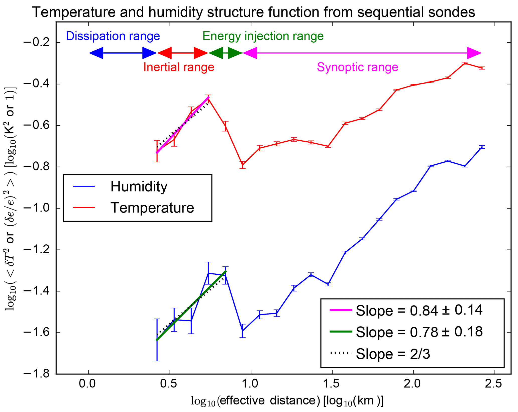
Within the inertial range, the structure function typically exhibits a power law behavior with a two third exponent following Kolmogorov's theory of turbulence (Frisch, 1995). The two-thirds law from Kolmogorov states that

$$\begin{array}{}\text{(1)}& \langle \left(\mathit{\delta }v\right(l){)}^{\mathrm{2}}\rangle =C{\mathit{\epsilon }}^{\mathrm{2}/\mathrm{3}}{l}^{\mathrm{2}/\mathrm{3}},\end{array}$$

where v is a parameter measured in the fluid, C is a universal dimensionless constant, which needs to be determined from experimental data, and l is the distance between the points where the parameter difference is determined. The mean energy dissipation rate per unit mass, ε, effectively constitutes a measure of the intensity of turbulence. The measurements from sequential sondes, within the inertial range, follow this law remarkably well. The measured slopes are 0.84±0.14 and 0.78±0.18 for temperature and water vapor, respectively. These values are consistent with the theoretical one of two thirds.

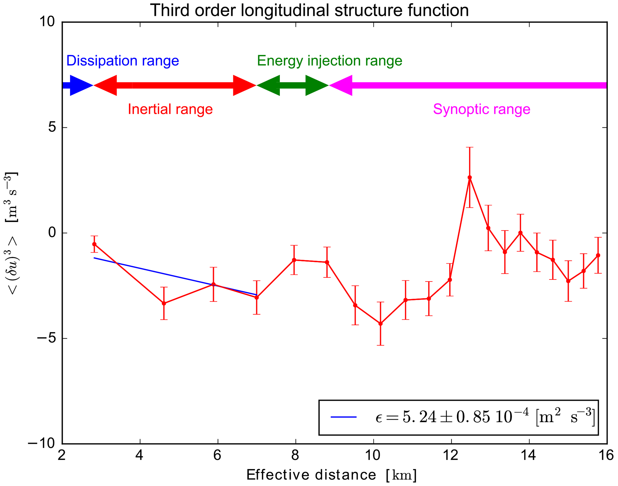
To determine the constants in the above equation, the four-fifths law from Kolmogorov's theory (Frisch, 1995) is needed

$$\begin{array}{}\text{(2)}& \langle \left(\mathit{\delta }{v}_{\parallel }\right(l){)}^{\mathrm{3}}\rangle =-{\displaystyle \frac{\mathrm{4}}{\mathrm{5}}}\mathit{\epsilon }l,\end{array}$$

where v_∥ is the velocity in the direction of the flow. This quantity can be estimated from the radiosonde measurements by using the u wind component. This relationship is shown in Fig. 2. A value of ε=5.2 cm² s⁻³ fits well within the inertial range. This is typical of the lower troposphere, with values usually between 1 and 10 cm² s⁻³ (Chen, 1974).

3 Radiative transfer modeling

We can now try to answer the question whether turbulence can have a significant effect on the RTM calculations. In this section, the radiance originating from a single profile will be compared to the one generated from this same profile perturbed by turbulence.

The turbulent perturbation from a single profile will be calculated by means of averaging a Taylor expansion of the radiances over the inertial range within the field of view of the instrument. The humidity variable used in this Taylor expansion will be the same as the one used in the structure function plot, Fig. 1. To simplify the notation, this variable will be defined as $\mathit{\delta }R\equiv \mathit{\delta }e/e$. The full Taylor expansion would then read,

$$\begin{array}{ll}{\displaystyle }& {\displaystyle }\langle \mathit{\delta }B\rangle \approx \sum _{i=\mathrm{1}}^{\mathrm{All}\mathrm{Levels}}{\displaystyle \frac{\partial B}{\partial R_i}}\langle \mathit{\delta }{R}_i\rangle +{\displaystyle \frac{\partial B}{\partial T_i}}\langle \mathit{\delta }{T}_i\rangle \\ {\displaystyle }& {\displaystyle }+{\displaystyle \frac{\mathrm{1}}{\mathrm{2}}}{\displaystyle \frac{{\partial }^{\mathrm{2}}B}{\partial R_i^{\mathrm{2}}}}\langle (\mathit{\delta }{R}_i{)}^{\mathrm{2}}\rangle +{\displaystyle \frac{{\partial }^{\mathrm{2}}B}{\partial T_i\partial R_i}}\langle \mathit{\delta }{T}_i\mathit{\delta }{R}_i\rangle \\ \text{(3)}& {\displaystyle }& {\displaystyle }+{\displaystyle \frac{\mathrm{1}}{\mathrm{2}}}{\displaystyle \frac{{\partial }^{\mathrm{2}}B}{\partial T_i^{\mathrm{2}}}}\langle (\mathit{\delta }{T}_i{)}^{\mathrm{2}}\rangle ,\end{array}$$

where we have made the important assumption that the correlation between different levels is 0, i.e.,

$$\begin{array}{}\text{(4)}& \langle \mathit{\delta }{B}_i\mathit{\delta }{B}_j\rangle =\langle \mathit{\delta }{T}_i\mathit{\delta }{B}_j\rangle =\langle \mathit{\delta }{T}_i\mathit{\delta }{T}_j\rangle =\mathrm{0}\text{ if }i\ne j.\end{array}$$

Figure 2 Third order longitudinal structure function for u.

As will be shown later in Sect. 4 and Figs. 4 and 5, the terms in Eq. (3) involving the temperature are negligible, leaving the simplified solution,

$$\begin{array}{}\text{(5)}& \langle \mathit{\delta }B\rangle \approx \sum _{i=\mathrm{1}}^{\mathrm{All}\mathrm{Levels}}{\displaystyle \frac{\mathrm{d}B}{\mathrm{d}{R}_i}}\langle \mathit{\delta }{R}_i\rangle +{\displaystyle \frac{\mathrm{1}}{\mathrm{2}}}{\displaystyle \frac{{\mathrm{d}}^{\mathrm{2}}B}{\mathrm{d}{R}_i^{\mathrm{2}}}}\langle (\mathit{\delta }{R}_i{)}^{\mathrm{2}}\rangle .\end{array}$$

The first (linear) term in this equation is proportional to the Jacobian. This result indicates that given a deviation of the mean humidity field of 0, the mean deviation in brightness temperature is directly proportional to the second derivative of the brightness temperature with respect to humidity.

It is now possible, by means of Eq. (5), to estimate in practice the magnitude of the brightness temperature deviations. Note that the average in this equation is taken over the complete field of view of the instrument, typically 10 km at nadir for SAPHIR. The value of fluctuations in humidity, 〈(δR_i)²〉, will vary within the field of view (inertial range in Fig. 1) and with turbulence intensity (ε in Eq. 1). To simplify, an approximate average is taken for the humidity fluctuations as a function of turbulence intensity. A value of 〈(δR_i)²〉=0.05 is adopted for a turbulence intensity of ε=5 cm² s⁻³, both parameters approximated from the values obtained from sonde measurements as in Figs. 1 and 2. For other turbulence intensities, humidity fluctuations are scaled following Eq. (1), expressing ϵ in units of cm⁻² s⁻³,

$$\begin{array}{}\text{(6)}& \langle (\mathit{\delta }{R}_i{)}^{\mathrm{2}}\rangle \approx \mathrm{0.05}(\mathit{ϵ}/\mathrm{5.0}{)}^{\mathrm{2}/\mathrm{3}}.\end{array}$$

The same arguments can also be applied to the temperature field fluctuations, in which case, the full Taylor expansion equation should be used (Eq. 3).

A single profile is chosen from a typical tropical location at Manus island and it is extracted from ECMWF analyses. The reason to choose a tropical profile is because high turbulence in the high troposphere seems to be more likely to happen in these regions. The profile has 50 levels from the lowest level at 1010 hPa to the highest one at $\mathrm{5}\times {\mathrm{10}}^{-\mathrm{3}}$ hPa. Figure 3 illustrates the lower levels of the profile, the Jacobians and the second derivatives for a few close to SAPHIR frequencies. Satellite zenith angle is fixed to 60^∘. Derivatives of the brightness temperature are calculated by finite differences using the AM 9.2 radiative transfer model (Paine, 2016). Final results of the brightness temperature differences are shown in Fig. 4.

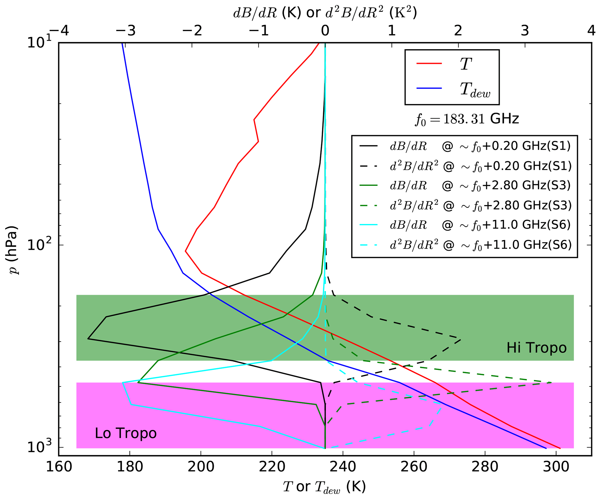
Figure 3 Temperature and humidity profiles, as dew point temperature, used in this paper. Highlighted are the regions denoted as “Hi Tropo” and “Lo Tropo” in Fig. 4. Jacobians, dB∕dR, and second derivatives, d²B∕dR², of brightness temperature vs. humidity for a few close to SAPHIR channels are also plotted. Precise frequencies are: 183.50 GHz ≈ S1 channel, 186.10 GHz ≈ S3 channel and 194.30 GHz ≈ S6 channel.

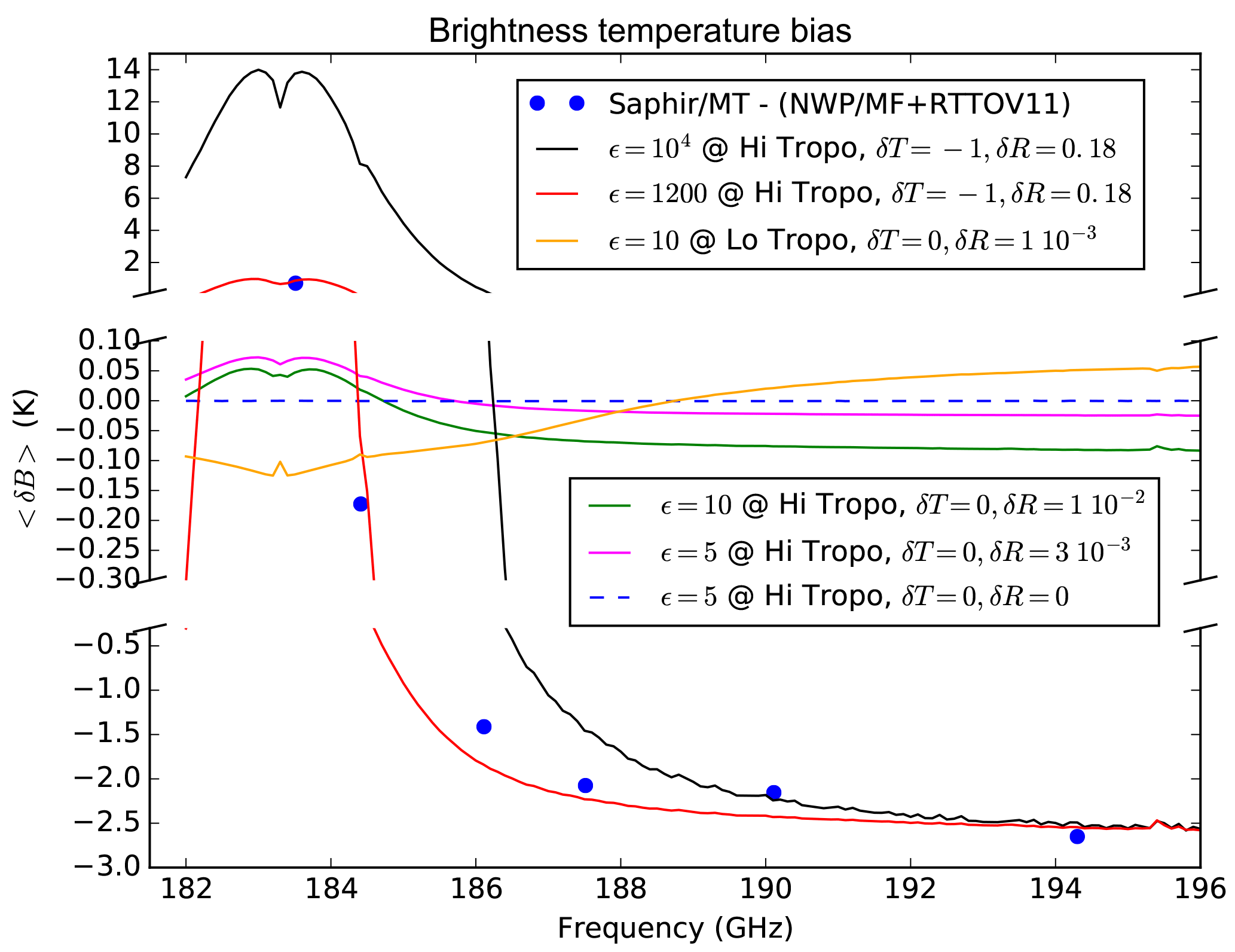
Figure 4 Brightness temperature deviations calculated for different levels in the troposphere (as shown in Fig. 3), various turbulence intensities, ε in cm² s⁻³, and adjusted offsets in temperature and humidity. Blue dots are values of observed minus calculated brightness temperatures between the SAPHIR Megha-Tropiques instrument vs. Météo France NWP profiles plus the RTTOV v11 RTM (from Brogniez et al., 2016).

4 Discussion

4.1 Simulations

Simulations comparing radiances with turbulence vs. radiances without them are shown in Fig. 4. Results show differences in brightness temperatures when locating turbulence in different layers in the troposphere, with various turbulent intensities and with varying perturbations in temperature and humidity. Several interesting features can be observed as follows.

• When only turbulent perturbations in temperature are considered, 〈(δT_i)²〉≠0, the results in brightness temperature difference are very small and nearly negligible (dashed blue line). In this case, the full Taylor expansion formula is needed (Eq. 3).

• With low turbulent intensities in humidity, ε=5 cm² s⁻³, located in the high troposphere, between 170 and 370 hPa, and with an offset in humidity of $\mathit{\delta }R=\mathrm{3}\times {\mathrm{10}}^{-\mathrm{3}}$ (magenta line) the effects are positive in frequencies near the center of the 183 GHz line and negative further away. The brightness temperature differences are of only a few tenths of a kelvin.

• With higher turbulent intensities in humidity, ε=10 cm² s⁻³, located in the high troposphere (green line) results are slightly higher than in the previous case.

• With the highest observed turbulent intensities in the low troposphere, ε=10 cm² s⁻³, and locating the humidity turbulent simulations in the low troposphere, between 480 and 1010 hPa, and with an offset in humidity of $\mathit{\delta }R={\mathrm{10}}^{-\mathrm{2}}$ (orange line) the biases show a different behavior, they are negative in frequencies near the center of the 183 GHz line and positive further away. The brightness temperature differences are of only a few tenths of a kelvin.

• Locating the turbulence in the high troposphere and fitting the parameters to follow the observed data (blue dots) the results are ε=1200 cm² s⁻³, $\mathit{\delta }T=-\mathrm{1}$ K and δR=0.18 (red line). The brightness temperature differences are of the order of a few kelvin. The simulations fit very well the observed data. Also, offsets in temperature and humidity are necessary. This offset is positive and is quite high, meaning that the average value of humidity in nature is actually higher than in the spatially uniform model.

• With the highest observed turbulent intensities in the high troposphere, ε=10⁴ cm² s⁻³, and locating the turbulence in the same high troposphere, the brightness temperature differences are up to several tens of kelvin (black line).

4.2 Behavior of the different terms

The orders of magnitude and the behavior of the various terms in both Taylor expansions (Eqs. 3 and 5) will be analyzed here. The cross-correlation term in humidity and temperature in Eq. (3) is not directly described in Kolmogorov's theory of turbulence, and, therefore, it is not easy to estimate. Since we are only interested, at this stage, in estimating the order of magnitude, the gross assumption that the cross-correlation is equal to the product of both variations can be made,

$$\begin{array}{}\text{(7)}& \langle \mathit{\delta }{T}_i\mathit{\delta }{R}_i\rangle \sim \langle \mathit{\delta }{T}_i\rangle \langle \mathit{\delta }{R}_i\rangle .\end{array}$$

Results are shown in Fig. 5. The following features can be observed.

• Using the full Taylor expansion (Eq. 3) if only an offset in temperature is introduced (orange line), the brightness temperature is displaced with hardly any frequency dependence.

• Using the full Taylor expansion (Eq. 3) if only a humidity offset is introduced (blue line), the brightness temperature is displaced, but there are also differences of a few kelvin which depend on the frequency.

• Placing high values of turbulence in the high troposphere and no perturbations in temperature or humidity, the effects of turbulence can be clearly seen (green line). It generates an overall positive displacement in brightness temperature of several kelvin and it is very strongly dependant on the frequency. The full Taylor expansion formula has been used here (Eq. 3).

• To shift this curve down in order to fit the observed data (blue dots), an offset is required. This can be achieved with a temperature or a humidity bias (red line). In this paper, both have been utilized ($\mathit{\delta }T=-\mathrm{1}$ K, δR=0.18), but any other appropriate combination of offsets would also fit the data. An offset in humidity partially compensates the turbulence effect, as can be seen from the differences between the red and the green line. The full Taylor expansion formula has been used here (Eq. 3).

• To verify that the temperature terms from Eq. (3) are negligible, the same parameters as in the red line are used to plot the reduced Taylor expansion from Eq. (5) (black line). Due to their small difference, the black and red curve are nearly indistinguishable. The black line in this plot is identical to the red line from Fig. 4.

• Finally, as a simple test to check whether temperature and humidity offsets would fit the observed data by themselves, without any turbulence effect, the purple curve is shown. This curve comes close to the observed data (blue dots), but with unreasonable values of temperature and humidity offsets ($\mathit{\delta }T=-\mathrm{8}$ K, $\mathit{\delta }R=-\mathrm{0.8}$).

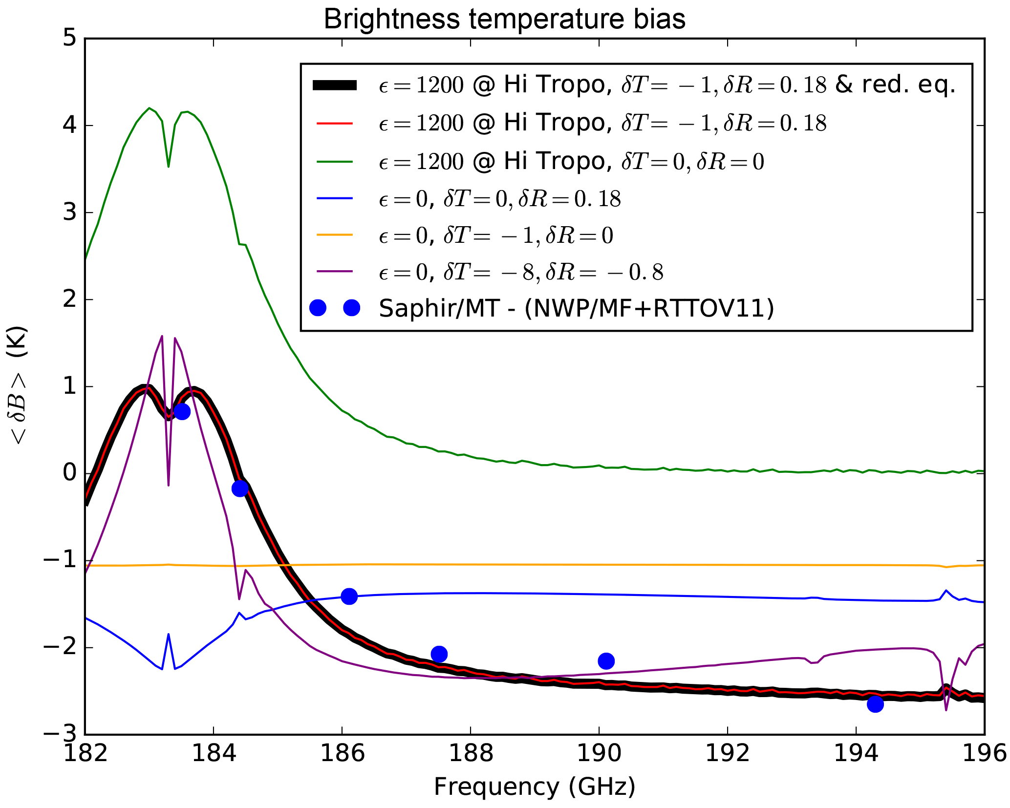
Figure 5 Same as Fig. 4, but setting parameters to analyze the behavior of the different terms in the Taylor expansions from Eqs. (3) and (5). The full Taylor expansion (Eq. 3) is used to calculate all the lines in this plot except for the black line, which uses the reduced Taylor expansion from Eq. (5).

5 Conclusions

Effects of turbulence in radiative transfer modeling stems from the fact that the process is highly non-linear. In other words, the average of the radiances coming from different atmospheric columns located within an instrument field of view can potentially be different from the radiance obtained using the average of all the atmospheric columns. Effects of turbulence in temperature fields seem to have a low impact in the radiative transfer modeling (dashed blue line of Fig. 4). Humidity turbulent effects seem to significantly affect the radiance biases by as much as several kelvin.

Turbulence simulations can match observed biases as summarized by Brogniez et al. (2016). Biases are positive close to the center of the absorption band and negative at the wings. To achieve this match, turbulence has to be of high intensity and located in the high troposphere (red line in Fig. 4). These high turbulence phenomena usually occur in places with clear air turbulence, regular or severe storms and cumulus clouds (Chen, 1974).

Turbulence simulations placed at the low troposphere create biases which have an opposite behavior as to the ones originating at the high troposphere. In other words, negative in the center of the absorption band and positive at the wings (orange line in Fig. 4).

Note that the calculations presented here have been made with just one atmospheric profile and one satellite zenith angle since the sole purpose of the exercise is to test whether the turbulence effect hypothesis can plausibly explain the observed biases. Biases shown in more general studies, such as Brogniez et al. (2016), are usually the result of an average of many different cases at different locations. To verify precisely that these biases do originate from turbulence effects, many different cases at different locations should be analyzed to finally calculate a global bias, which can then be compared with the measured ones. Turbulence effects will also depend strongly on each scene analyzed. Furthermore, in this paper, turbulence properties have been measured with radiosondes at mid-latitudes (Sodankylä and Lindenberg) and this is being extrapolated to other regions by only changing the turbulence intensity (mean energy dissipation rate per unit mass, ϵ). A more local measurement of turbulence would better characterize the scenes under scrutiny.

Bobryshev et al. (2018) have also tried to reconcile the biases found between microwave satellite instruments and sonde measurements plus radiative transfer modeling. By correcting dry biases from sonde measurements and selecting fields of view which are unaffected by clouds and are spatially homogeneous they achieved agreement between satellite observations and sonde measurements. They are, in practice, selecting scenes with low turbulence such that its effects in radiative transfer modeling are not significant. These results are therefore consistent with the ones presented in this paper.

In summary, turbulence within the field of view of microwave instruments seems to have a significant effect in the modeling of radiative transfer, which, if ignored can give rise to significant biases up to several kelvin in the 183 GHz band. These biases are frequency dependant. To confirm this hypothesis, more precise and further modeling and its corresponding comparisons with measurements at different frequencies in the microwave and the infrared, in this latter case, under clear sky conditions, would be needed. Coincident turbulence measurements of the atmosphere might also be necessary to solve the problem.

Another, additional conclusion that can be envisaged from these results is that when comparing atmospheric profiles with sondes for precise calibration or validation either a turbulent term should be added in the uncertainty budget or dual sequential radiosondes should be used. This will be the subject of a future paper.