the Creative Commons Attribution 4.0 License.
the Creative Commons Attribution 4.0 License.
 | 07 Dec 2018
Analysis of a warehouse fire smoke plume over Paris with an N2 Raman lidar and an optical thickness matching algorithm
Patrick Chazette
Julien Totems
A smoke plume, coming from an accidental fire in a textile warehouse in the north of Paris, covered a significant part of the Paris area on 17 April 2015 and seriously impacted the visibility over the megalopolis. This exceptional event was sampled with an automatic N2 Raman lidar, which operated 15 km south of Paris. The industrial pollution episode was concomitant with the long-range transport of dust aerosols originated from the Sahara, and with the presence of an extended stratus cloud cover. The analysis of the ground-based lidar profiles therefore required the development of an original inversion algorithm, using a top-down aerosol optical thickness matching (TDAM) approach. This study is, to the best of our knowledge, the first lidar measurement of a fresh smoke plume, emitted only a few hours after an accidental warehouse fire. Vertical profiles of the aerosol extinction coefficient, depolarization ratio, and lidar ratio are derived to optically characterize the aerosols that form the plume. We found a lidar ratio close to 50±10 sr for this fire smoke aerosol layer. The particle depolarization ratio is low, %, suggesting the presence of either small particles or spherical hydrated aerosols in that layer. A Monte Carlo algorithm was used to assess the uncertainties on the optical parameters and to evaluate the TDAM algorithm.
- Article
(3696 KB) - Full-text XML
-
Supplement
(443 KB) - BibTeX
- EndNote


Accidental fires cause casualties and significant property damages. In France, one house fire occurs every 2 min, adding up to 263 000 domestic fires each year, causing about 100 deaths and 10 000 injuries (http://iaaifrance.fr/, last access: 3 December 2018). These fires also emit large amounts of gases and aerosols, which are detrimental to human health and degrade visibility. The aerosols have a notable role in cloud formation and in the atmospheric radiative budget (Kanitz et al., 2013). Concerning accidental fires, the meteorological situation has an important role in fire and smoke propagation, especially wind force and direction. In return, fires influence the dynamics and the chemistry of the atmosphere, mainly in the atmospheric boundary layer (ABL) and the low free troposphere. Modelling tools are needed to predict regional aerosol emissions from large fires and analyse emergency policy options. However, the characterization of fire emissions remains incomplete, mainly due to the difficulty of obtaining young smoke samples. Their unpredictability poses an obvious challenge for the performance of chemical and meteorological measurements.
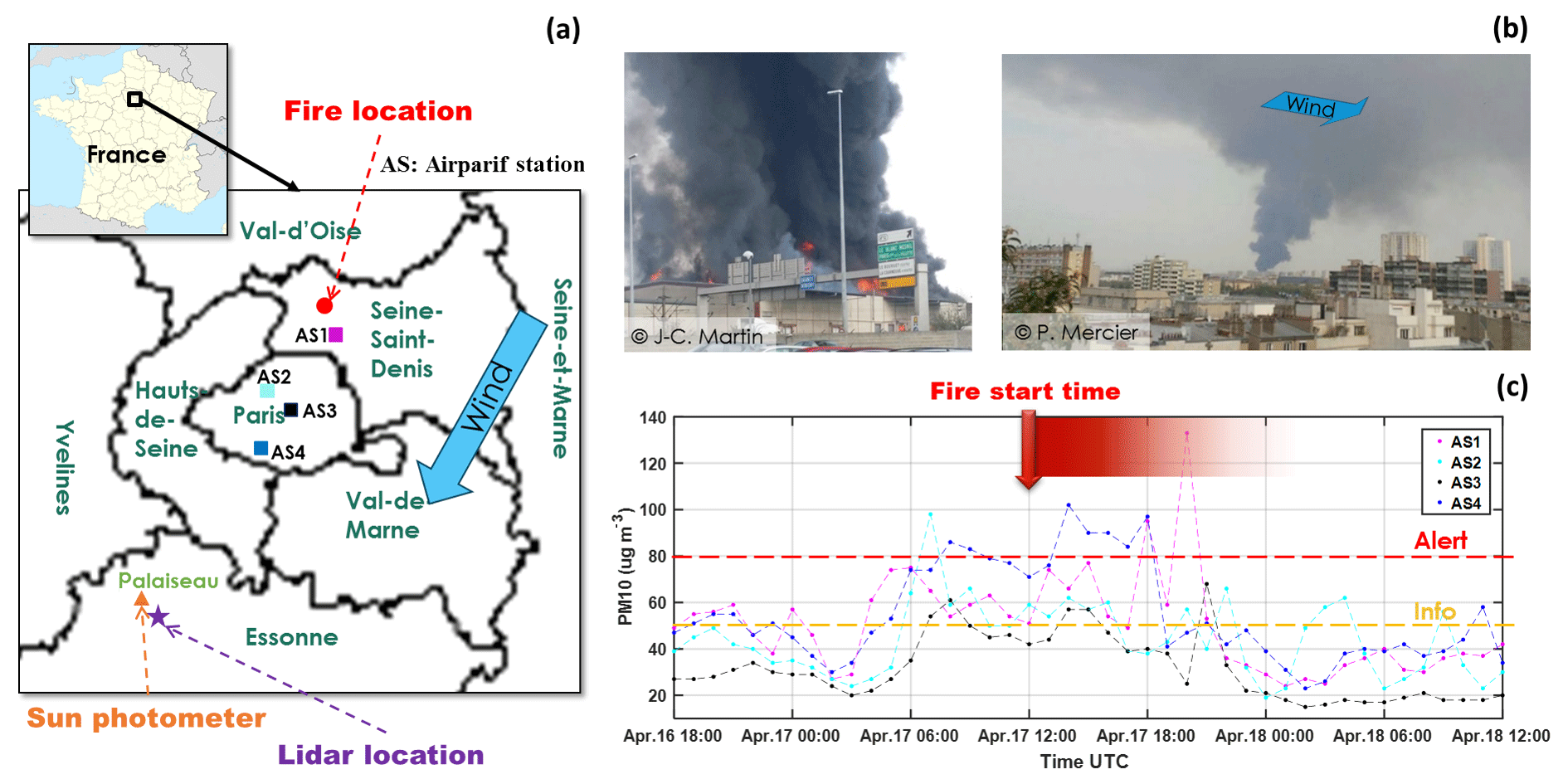
Figure 1(a) Locations of the textile warehouse on fire (red circle), of lidar instruments (purple star), and of the sun photometer (orange triangle); (b) photo of the smoke plume from near (left) and far (right) distance; (c) in situ measurements of PM10 from four Airparif stations (locations shown in a). The alert and information values are also given by the red and yellow dashed lines.
Lidar is an efficient technique for the detection of various types of particles along the altitude, such as ash, air pollution, dust, and biomass burning aerosols (Ansmann et al., 2012; Chazette et al., 2007, 2012; Mattis et al., 2010; Müller et al., 2007; Royer et al., 2011; Weitkamp, 2005). Lidar-derived parameters can be effective constraints for chemical transport models (Binietoglou et al., 2015; Haustein et al., 2009; Wang et al., 2014). Raman lidars, in particular, are becoming well-established tools that are used in the study of numerous areas of importance in the atmospheric sciences (Ansmann et al., 1992; Behrendt et al., 2007; Di Girolamo, 2004; Whiteman, 2003). The use of both Raman- and elastic-backscatter lidar signals allows the independent retrieval of the aerosol extinction and backscatter coefficients (e.g. Ansmann et al., 1992). This technique also enables the retrieval of the extinction-to-backscatter ratio, also called lidar ratio (LR), and the linear particle depolarization ratio (PDR). The LR is considered an important criterion to analyse atmospheric aerosols, as it depends on their single scattering albedo and backscatter phase function, and is thus a function of size distribution and chemical composition. The PDR provides information on the shape of the scattering particles, allowing the identification of several aerosol types.
Raman lidar data processing remains a complex matter. Three kinds of algorithms are available: (1) single-layer aerosol optical thickness (AOT) constrained Klett inversion, which is a conventional approach based on the Klett algorithm (Klett, 1981), using the N2 Raman AOT to choose a column-equivalent LR (CLR; Ansmann et al., 1990, 1992); (2) standard Raman inversion, based on the numerical derivative of the N2 Raman channel to retrieve the extinction profile, but introducing noise (Pappalardo et al., 2004; Whiteman, 1999); (3) Raman-constrained regularization, such as the Tikhonov method (Tikhonov and Arsenin, 1978), solving the lidar equation to retrieve the aerosol extinction and backscatter coefficient profiles simultaneously (Royer et al., 2011; Shcherbakov, 2007). As an intermediate, Ansmann (2006) applied the two-layer approach of the Klett method to determine a pair of column lidar ratios for the boundary layer and for the lofted free tropospheric aerosol layer. Yet all these approaches are based on the premise that the elastic channel maximum range can reach an altitude where the backscattered signal is dominated by its molecular contribution (with pure Rayleigh scattering), so as to normalize the signal. We will hereafter call this altitude the Rayleigh zone. One cannot invert the lidar profile if low clouds obstruct the signal or if aerosol layers are present within the hypothetic Rayleigh zone. Moreover, in the presence of a plume from a large fire, it is very common to observe the formation of clouds inside or at the top of the plume, since a fire releases large amounts of water vapour in the atmosphere. The strong AOT of the plume may significantly limit the lidar maximum range, inducing a marked decrease of the signal-to-noise ratio (SNR) in the Rayleigh zone. Thus, it may be more interesting to find a reference at a lower altitude to invert the lidar vertical profiles.
On 17 April 2015, we were able to sample a freshly emitted smoke plume from an accidental fire using a N2 Raman lidar located at Palaiseau (48∘42′23 N, 2∘13′22 E), ∼ 15 km south of Paris. This fire, of great magnitude, occurred ∼ 5 km north of Paris in a 12 000 m2 textile warehouse located in the commercial area of La Courneuve (48∘55′52 N, 2∘23′52 E). The warehouse was totally burned down. To analyse the lidar data recorded during this event, we had to develop a new Raman lidar inversion approach for ground-based measurements, which we call hereafter the top-down aerosol optical thickness matching (TDAM) approach, based on the Klett algorithm. TDAM makes it possible to retrieve the LR profiles with more vertical detail, even when a Rayleigh zone cannot be reached by the lidar.
This paper is organized as follows. In Sect. 2, we introduce the accidental fire event and lidar instrument. In Sect. 3 we recall the theory by presenting the equations and the basic variables associated with N2 Raman lidar analysis. In the same section, we then present some standard inversions and introduce our new TDAM approach. An uncertainty study is also proposed at the end of that section. The application of TDAM to the warehouse fire smoke plume that passed over the ground-based lidar is discussed in Sect. 4. Section 5 is devoted to the conclusion.
2.1 Accidental fire of a warehouse
On 17 April 2015, a violent fire broke out around 14:00 local time (12:00 UTC), in a 12 000 m2 two-storey textile and footwear warehouse in La Courneuve, Seine-Saint-Denis, France (48∘55′52 N 2∘23′52 E; Fig. 1). The plume quickly rose in the lower free troposphere, just above the ABL, by pyro-convection. Black smoke covered the north area of Paris, as shown in Fig. 1b. With a wind speed of ∼ 22 km h−1, the smoke plume rapidly spread from the north–north-east to the south–south-west of Paris. There were no casualties, but property damages were assessed to be around EUR 40 million. Around 150 firemen and 40 fire trucks participated in the fire fighting. The burning materials were mainly plastic, cloth, wood, paper, etc. (video of the fire at https://www.youtube.com/watch?v=0hC52-pEmu8, last access: 3 December 2018). The societal impact was also rather important, as the traffic was severely disrupted on numerous motorways and railways of the northern Paris area for ∼10 h. A strong smell of smoke and burned plastic spread throughout Paris from that fire and reached the location of the ground-based lidar around 17:00 local time.
2.2 Instrument: N2 Raman lidar
The N2 Raman LAASURS (Lidar for Automatic Atmospheric Surveys using Raman Scattering) was put into operation in Palaiseau (48∘42′23 N 2∘13′22 E; Fig. 1a), south-west of Paris, to sample the fire smoke plumes. The direct distance between the locations of the fire and the lidar site is ∼28 km.
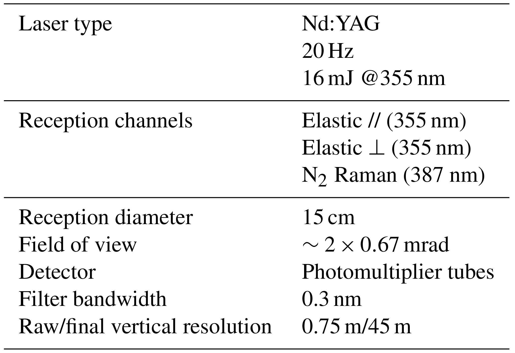
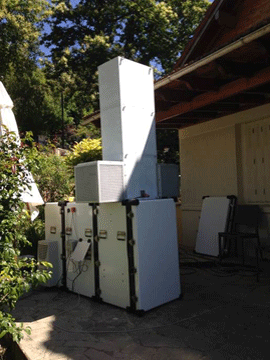
LAASURS is already well described and validated by Royer et al. (2011) and Chazette et al. (2012). Its characteristics are summarized in Table 1; it can be remotely controlled and can work under almost all weather conditions thanks to an air conditioning system and a funnel equipped with air blowers above the optical windows (Fig. 2). LAASURS uses an emission wavelength of 355 nm and is designed to fulfil eye-safety conditions at its output. It is composed of two reception channels: one dedicated to the measurement of the co- and cross-polarized signals at ∼355 nm and the other to the inelastic nitrogen Raman backscattered signal at ∼387 nm. Using a high-speed digitizer card with 200 MHz sampling frequency, it enables the retrieval of aerosol optical properties and atmospheric structures with an initial/final resolution of 0.75/45 m along the line of sight.
2.3 Raw observations from lidar
The 10 h lidar observations of the atmosphere following the fire event are presented in Fig. 3, using the temporal evolutions of vertical profiles of both the elastic range-corrected signal () and volume depolarization ratio (VDR). Three main aerosol layers can be easily located in the low troposphere: (i) the ABL during the day and the nocturnal layer (NL) during the night, under ∼1.2 km a.m.s.l. (above mean see level), (ii) a thin non-depolarizing layer close to 1.2 km a.m.s.l. with a strong backscatter signal (smoke layer), and (iii) a more depolarizing layer between 1.8 and 3 km a.m.s.l. The lidar signals are drawn with a time resolution of 1 min and a vertical resolution of 45 m. During this event, there are a significant number of profiles impacted by low clouds, which makes the lidar inversion a challenge. Also, a good vertical resolution of lidar parameters is required to investigate the very thin smoke layer.
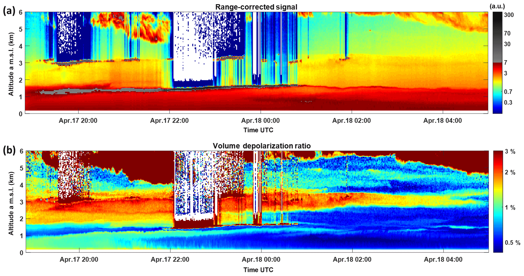
Figure 3Time series, from 17 April 2015 at 18:50 UTC to 18 April 2015 at 05:00 UTC, of the profiles of (a) elastic range-corrected signal () and (b) volume depolarization ratio (VDR).
3.1 Basic lidar theory
Starting from the well-known lidar equation (Measures, 1984), the backscattered lidar signal can be corrected for the sky background, the solid angle, and the overlap function to obtain the range-corrected lidar signal (RCLS) Sλ. The RCLS of the elastic (E) and the Raman (R) channel are expressed at altitude z as
where λE and λR designate the emitted wavelength (λE=354.67 nm) and the first Stokes vibrational N2 Raman wavelength (λR=386.63 nm), respectively. The instrumental constant Kλ contains all altitude-independent system parameters. is the nitrogen molecule number density, is the range-independent differential Raman cross section for the backward direction. α and β are the molecular (mol) or aerosol (aer) extinction and backscatter coefficients, respectively. The molecular extinction (αmol) and backscatter (βmol) coefficients can be calculated from climatological air mass models or radiosonde measurements. They are determined in this study with a polynomial approximation as in Nicolet (1984) using a reference atmospheric density calculated from ancillary measurements (Chazette et al., 2010); is expressed as , with the King factor of air kf (King, 1923). The aerosol extinction (αaer) is assumed to be proportional to λ−Å, where the Ångström exponent Å (Ångström, 1964) is considered to be a constant depending on the aerosol nature. This value can be obtained from external data such as a sun photometer (Dubovik et al., 2002).
The aerosol optical thickness (AOT) between two altitudes zi and zj at the wavelength λ is defined as the integration of the aerosol extinction coefficient (AEC) on the altitude range [zi,zj] and can be derived directly using the Raman channel signal from Eq. (2) (Royer et al., 2011). For a chosen reference altitude (z0), the aerosol backscatter coefficient (ABC) at altitude z can be derived using either the ratio of the elastic signals, which is corrected from the molecular extinction contribution (Royer et al., 2011), or the ratio of the elastic and the Raman backscattered signals (Ansmann et al., 1992; Whiteman et al., 1992). An assumption about the reference value is needed. Usually, the reference altitude zref is chosen in a Rayleigh zone where the aerosol load is negligible; i.e. .
For lidar systems with co- and cross-polarized channels, the volumetric depolarization ratio (VDR) and linear particle depolarization ratio (PDR) can be derived following the procedure described in Chazette et al. (2012). As the PDR is a physical parameter retrieved with a high uncertainty when there are few aerosol particles, its calculation in this study is only performed for layers where the AEC is at least 0.01 km−1.
The lidar ratio (LR, also called particle extinction-to-backscatter ratio) is determined by the ratio of two unknowns, αaer and βaer, of the lidar equation. The LR depends on the complex refractive index, size, shape, and orientation of aerosols (Sasano et al., 1985). The main Raman inversion methods, yielding retrievals of LR, can be classified as three types of algorithms:
-
Single-layer AOT constrained Klett algorithm (Ansmann et al., 1990; Chazette et al., 2010; Dieudonné et al., 2015). The main error sources are well known and are mainly due to the vertical heterogeneity of the aerosol layers. The altitude-independent LR can be poorly representative of the actual LR profile, especially in the presence of multiple scattering layers composed of different types of aerosol (e.g. dust, pollution, and sea salt aerosols; Chazette et al., 2016). According to the sensitivity study carried out by Royer et al. (2011), for the same N2 Raman lidar presented in Sect. 2.2, the relative error on the altitude-independent LR ranges between 4 % and 18 % (16 % to 100 %) during night-time (daytime) for AOT values ranging from 0.1 to 0.5. Note that Ansmann (2006) found a difference in the altitude-independent LR of up to 20 % between the single-layer Klett solutions from spaceborne and ground-based lidar.
-
Standard Raman inversion. Mathematically, the AEC can be retrieved directly by differentiating the Raman-derived AOT profile. The distinction between algorithms of standard Raman inversion mainly concerns data-smoothing techniques and the evaluation of a numerical derivative (Pappalardo et al., 2004; Whiteman, 1999). Pappalardo et al. (2004) reported on the inter-comparison of several standard Raman inversions in the EARLINET network, which shows a mean deviation of LR within 20 % in the ABL, and within 15 % for a lofted aerosol layer.
-
Raman-constrained regularization. The regularization method most commonly used for Raman lidar processing is the Tikhonov regularization method (Royer et al., 2011; Shcherbakov, 2007). Shcherbakov (2007) reports a regularized algorithm (based on theory in Tikhonov and Arsenin, 1978), which improved the quality of the Raman lidar data processing compared to the standard Raman inversion. The retrieved LR profile has reduced root-mean-square errors but does not follow strong variations of the actual LR, especially at the boundaries between layers, and its smoothness gives a false impression of precision in zones with low signal-to-noise ratio (SNR). The Tikhonov approach is inherently an optimal estimator for the ABC, and not for the LR.
3.2 The top-down aerosol optical thickness matching (TDAM) algorithm
All the above approaches are based on the assumption that the aerosol load in the reference zone is negligible. However, because of clouds or thick aerosol loads or strong daylight background limiting the maximum usable range of the backscatter signals, or the presence of aerosols high in the free troposphere, there are cases in which a pure Rayleigh reference zone cannot be reached or does not exist (e.g. profiles with clouds or dust plumes above the ABL in this study). Moreover, we have discussed the limitations of regularized approaches that we cannot retrieve detailed information due to a vertical resolution unsuitable for a thin aerosol layer (e.g. the warehouse fire smoke aerosol layer (SAL) in this study). For ground-based N2 Raman lidar, a new algorithm has been developed to solve these problems and will be described in this section. In the following, the parameters without subscripts relate to the emitted wavelength (λE).
3.2.1 Reference zone and related optical parameters
The lidar profile is shared in several atmospheric layers indexed from i=1 to n, with the lowest index (i=1) corresponding to the maximum usable range of the signal and i increasing downwards to the ground level. Note that the layers are not necessarily equidistant. Whether the Raman channel reaches a pure Rayleigh zone or not, we choose the reference zone in the altitude range of [z1, z0], named as the first altitude interval, in which the AEC is considered as constant against the altitude (Fig. 4). Figure 5 gives an illustration of the method, using an actual lidar profile acquired during the fire smoke event (at 21:20 UTC). To estimate the AEC in the reference zone, due to a weak SNR, a least mean square approach is applied on the normalized N2 Raman lidar signal, after correction of the molecular contributions:
as proposed by Chazette et al. (2016). This ratio is proportional to the aerosol transmission in the first altitude interval, where the AEC is considered as constant, so that
Hence, the estimator of the AEC at the reference altitude is derived from
The computation of the LR in the first altitude interval (LR1) needs a second altitude interval [z2, z1], with z2 < z1. The altitude z2 is chosen to verify the following constraint on the partial AOT (PAOT) between z2 and z0:
The PAOT is derived from the Raman channel profile. The ABC at the reference altitude is given by
It is used as an initial value to constrain the Klett inversion (e.g. Eq. 12 in Royer et al., 2011). We assume that LR2=LR1 between z2 and z0. Hence, an analytical solution exists and is given by
where is the ratio of elastic lidar signal after correction of the molecular transmission:
If the solution does not converge to plausible LR values (between 20 and 120 sr), the second altitude interval is enlarged by one resolution step of the lidar profiles, and so on.
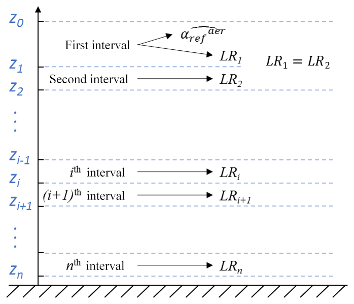
Figure 4Diagram of the ith (i=1, 2, …, n) altitude interval for the altitude range [] using the TDAM (top-down aerosol optical thickness matching) algorithm.
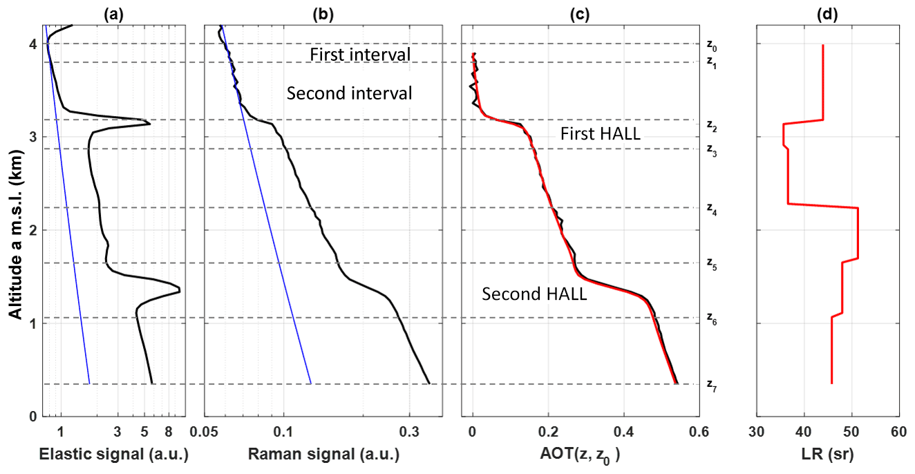
Figure 5Example for the demonstration of the TDAM (top-down aerosol optical thickness matching) algorithm, which is an actual lidar measurement at ∼ 21:20 UTC on 17 April (cf. Fig. 3). (a) Range-corrected elastic signal (black) with fitted molecular elastic signal (blue). (b) Range-corrected Raman signal (black) with fitted molecular Raman signal (blue). (c) Raman-derived AOT profile (black) with retrieved AOT profile using TDAM (red). Altitudes determining layers are shown by dotted lines, from which we can find the first altitude interval [z1, z0], the second altitude interval [z2, z1], and the ith altitude interval [zi+1, zi]. The two heavy aerosol load layers (HALLs) are also shown. (d) Retrieved LR profile using the TDAM algorithm.
3.2.2 Profiles of the aerosol optical parameter derived from the N2 Raman lidar
At this stage, the goal is to estimate profiles of and LR(z) using the LR and AEC previously retrieved at the reference altitude. Below the first and second altitude intervals, we identify n−2 successive homogeneous layers (see Fig. 4), and the LR inside each layer is assumed to be altitude-independent. Different methods can be used for this step. The easiest way is using a constant altitude interval (e.g. one LR value per 1 km). The altitude interval can also be defined considering a minimal value of PAOT (e.g. 0.1) to be reached in each interval. Indeed, the LR is meaningless for layers where the aerosol load is too small; this argues for sufficiently high PAOTs in each altitude range. Note that a thin layer i of strong PAOT can also significantly bias the retrieval of the LR value for the remaining n−i layers.
In this study, a more evolved method is used to define layers. Firstly, the existence of a “heavy aerosol load layer” (HALL) is checked using the slope of the range-corrected elastic signal, which has a better SNR than the Raman signal. In our example in Fig. 5, we identify two homogeneous aerosol layers, the first one between z3 and z2 and the second one between z5 and z6, as HALLs. Furthermore, we considered the ABL as one homogeneous layer. Secondly, we choose a constant AOT increment to determine the other homogeneous layers (Fig. 5c). In this study we select a value of 0.05 as a compromise between the final vertical sampling of LR and the computation time. Once the different layers, are defined, the inversion procedure starts.
The LR in the ith altitude interval, LRi=LR (zi, zi−1), can be derived following a procedure similar to the one presented in the previous section (Eq. 8), using the layer PAOT, . A LR profile, keeping the estimated values LR1, …, LRi−1 for the previous layers and testing for LRi in the new layer m values centred around LRi−1, is used for Klett inversion at this step. The LRi value best matching the Klett-derived PAOT to the measured value is chosen. We find that iterating (up to three times) with m=7 values and finer increments until the PAOT is found within 10−4 yields the best results in terms of precision and computation time.
This procedure is repeated for all the altitude intervals until the ground level is reached. The final estimate of the LR profile of the example considered in Fig. 5 is shown in Fig. 5d. Using the backward Klett method, we use this LR profile and the range-corrected elastic signal to compute the AOT profile (superimposed in red in Fig. 5c), which matches the AOT retrieved from the N2 Raman channel well.
The TDAM method may be of advantage if the retrieved backscatter coefficient profile indicates pronounced heterogeneities against altitude. It can be used extensively, even for daytime inversions, if the Raman maximum range is sufficient. However, this algorithm cannot be used to generate real-time quick look plots because it is relatively time-consuming (∼45 s computation time per profile).
3.3 Uncertainty sources
The uncertainties on aerosol optical properties retrieved from N2 Raman lidar measurements are mainly (i) bias linked to the effective vertical resolution, (ii) bias due to an inaccurate AEC in the reference zone, (iii) bias due to the assumed model of the molecular contribution, (iv) bias due to the assumed Ångström exponent, and (v) random error associated with the signal noise characterized by the SNR. The main uncertainties of the TDAM method will be discussed in the following. Uncertainty sources are assumed to be independent. Note that an error can also be introduced by temporal averaging during varying atmospheric extinction and scattering conditions, which will also be discussed in the next section for the warehouse fire smoke case study.
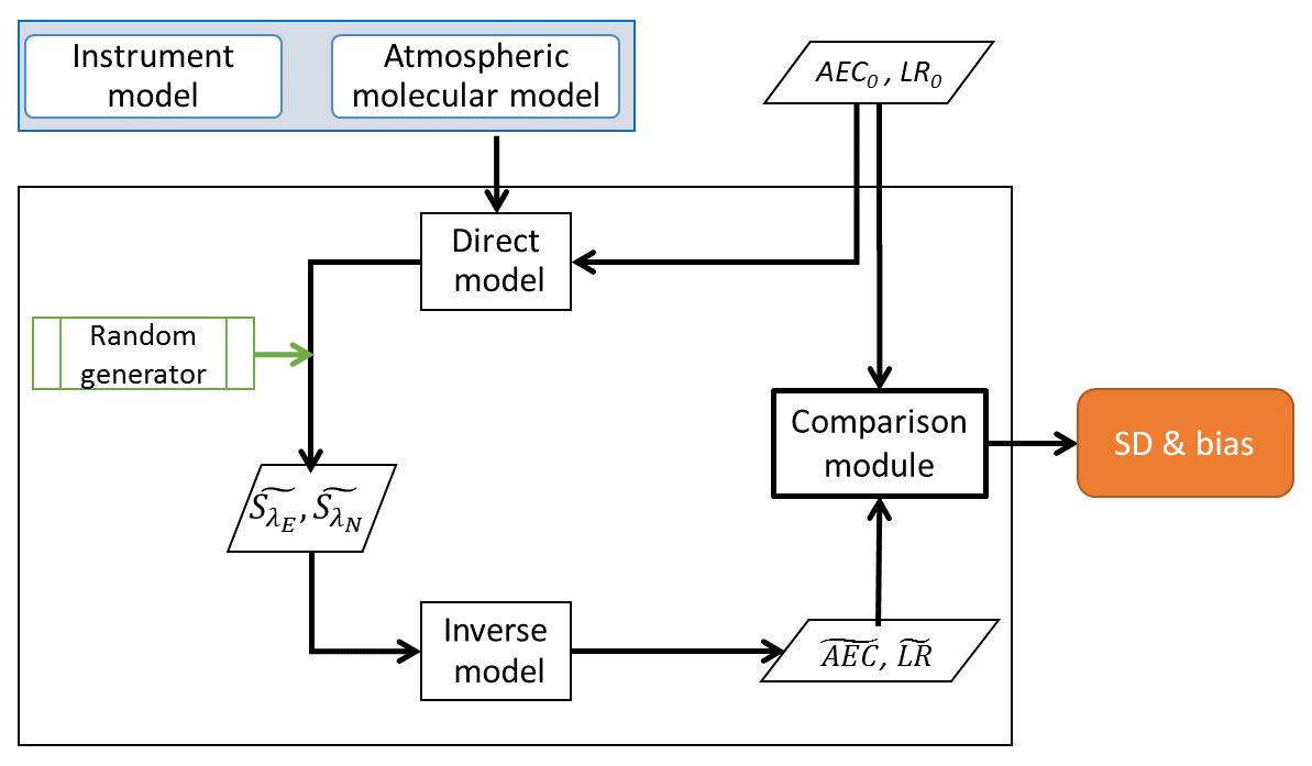
An end-to-end simulator was developed for the error study of the TDAM method, with the block diagram shown in Fig. 6. We developed a similar algorithm when studying the uncertainty sources for a spaceborne lidar dedicated to forest studies (Shang and Chazette, 2015). The input profiles of AEC and LR (AEC0 and LR0) can either be the ones retrieved from actual measurements or simulated profiles. They are used to simulate the backscattered lidar signals of both elastic () and Raman () channels through the “direct model”. The instrument parameters are adjusted using actual lidar signals. An atmospheric molecular model is used to provide the molecular contributions. The statistical error study is performed using a Monte Carlo approach as described in Chazette et al. (2001). The main sources of noise were taken into account considering normal statistical distributions, which are introduced by a normal random generator. For each statistical simulation, we used 100 draws, ensuring a normal distribution up to 1 standard deviation away from the mean value of the parameters. Each statistical realization of the lidar signals was then inverted by the “inverse model” to estimate the aerosol optical parameters. The comparison between these estimators and the initial values was then performed in the “comparison module” to retrieve the bias and standard deviations of the AEC, AOT, and LR.
3.3.1 Systematic errors
Systematic errors are mainly associated with the estimated input parameters. The uncertainty on the a priori knowledge of the vertical profile of the molecular contribution, as determined from ancillary data, has been assessed to be lower than 2 % as in Chazette et al. (2010) using a comparison between several radiosoundings. The Ångström exponent (Å) used in this study is 1.1. The Aerosol Robotic Network (AERONET) Level 2.0 product from the Palaiseau station near the lidar station (http://aeronet.gsfc.nasa.gov/, last access: 3 December 2018; Fig. 1) is considered, from which the visible (440–675 nm) mean Å on 17 April is found to be , representative of carbonaceous particles. Note that the Ångström exponent for Paris background aerosols is ∼1.5 (Chazette and Royer, 2017). Chazette et al. (2014) report that the residual relative uncertainty on LR due to Å ± 0.05 was calculated to be less than 3 %. The use of King factor kf=1 causes an overestimation of the molecular volume backscatter coefficient of 1.5 % at 355 nm (Collis and Russel, 1976). The error due to temporal averaging is not discussed here as it depends substantially on the atmospheric situation and should be studied separately for each study period.
3.3.2 Bias linked to the effective vertical resolution and AEC at the reference altitude
In this section, only simulated mean lidar signals are considered for the assessment of the biases linked to the effective vertical resolution and to the AEC at the reference altitude.
Firstly, we check the ability of the TDAM method to resolve two narrow and well-separated structures in the aerosol extinction profile. A step function proposed by Pappalardo et al. (2004) is used here to evaluate the effective vertical resolution. We took into account seven pairs of AEC profiles with Dirac peaks (the value is equal to zero everywhere except at the height of peaks), which are separated by 4, 6, 8, 12, 18, 22, 26, and 30 points between two peaks, respectively. In each case, the LR is set to be 40 for the top peak and 80 for the bottom peak. Using the TDAM method, we retrieved the and , which are then compared with the initial values (AEC0 and LR0). We find that TDAM resolves the two peaks of AEC separated by six points, which is related to an effective vertical resolution of 270 m in this study. The relative uncertainty on LR retrieval is ∼30 % for the pairs with a distance of four points, whereas other relative errors on LR are reasonable (<10 %) for pairs with a distance bigger than the effective vertical resolution.
Secondly, bias linked to the AEC at the reference altitude is evaluated. A heterogeneous atmosphere is considered here, with two superimposed layers with different aerosol loads and types (a Gaussian profile is chosen for each layer): (i) a smoke layer (LR0=50 sr) centred at 2 km a.m.s.l., with an AOT of 0.3 and a thickness of ∼500 m; (ii) a polluted boundary layer (LR0=80 sr), with an AOT of 0.2 from the ground to 1.7 km a.m.s.l. A background aerosol condition is also added, with a constant AEC of 0.05 km−1 from 0 to 6 km (LR0=80 sr).
We set the reference zone at 4–5 km, where the correct AEC () should be 0.05 km−1. Several artificial values from 0 to 0.2 km−1 were used for the inversion to assess the relative bias. We found that using 0 instead of 0.05 km−1 as the , the LR of the smoke aerosol layer (SAL) will be overestimated, with a relative bias of +40 % in this simulated case. When the is overestimated as 0.1 km−1 (0.14 km−1), the bias on the LR retrieval is % (−23 %). Note that if one uses the other three methods mentioned in Sect. 3.1 without a correct estimation of (i.e. 0 instead of the actual ), the LR retrieval will probably be overestimated.
3.3.3 Random error due to noise
In this section, we investigate the random error due to the noise on acquired signals, using the end-to-end simulator (Fig. 6) based on a Monte Carlo approach. The input profiles of AEC and LR (AEC0 and LR0 in Fig. 7a and b) are produced by smoothing actual measurements (17 April ∼ 20:20 UTC). The reference altitude was selected to be ∼4 km a.m.s.l., where the was 0.032 km−1 with a LR at the reference altitude (LRref) of 42 sr. A total of 100 draws were performed, with the noise level determined from the SNR of the actual lidar signals; the SNR at the reference altitude on Raman channel signal is found to be ∼184. One draw of simulated range-corrected elastic and Raman signal is shown in Fig. 7c and d. The aerosol layer at ∼1.5 km is related to our observed SAL, with an initial column-equivalent lidar ratio (CLR) value of 44 sr.
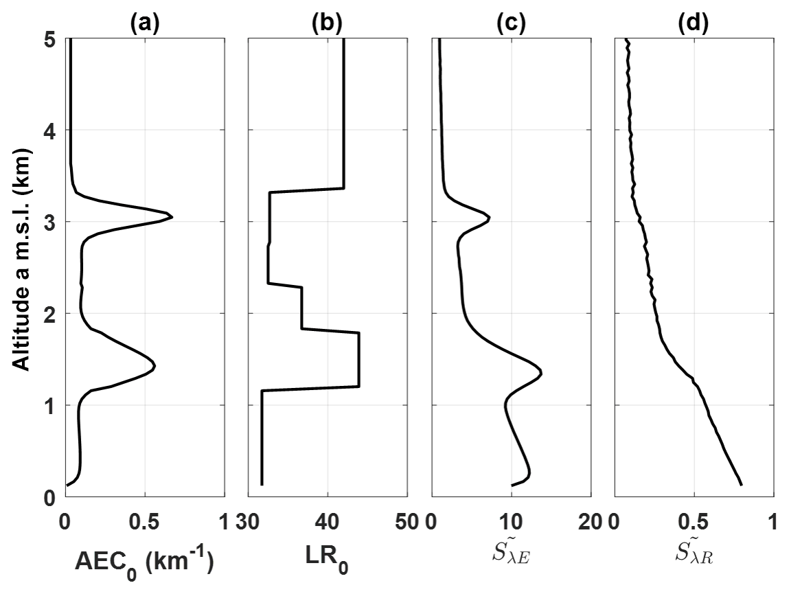
Figure 7Input profiles of (a) aerosol extinction coefficient (AEC0) and (b) lidar ratio (LR0) for the statistical error study. One draw of the 100 simulated profiles of range-corrected (c) elastic signal and (d) Raman signal is shown.
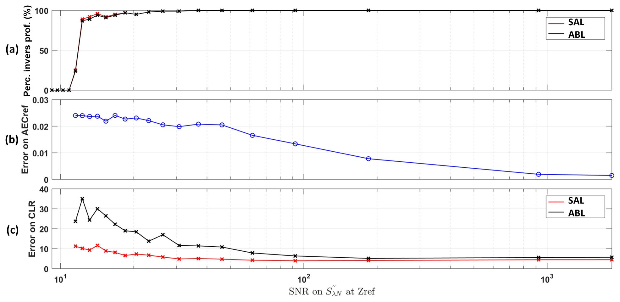
Figure 8(a) Percentage of inversible profiles, (b) errors on AECref (AEC at the reference altitude, , in km−1), and (c) errors on CLR (column-equivalent lidar ratio, in sr) due to random detection processes against the SNR at the reference altitude (zref) on the Raman channel () using the TDAM approach. Red and black lines show values for the SAL (smoke aerosol layer, between 1.1 and 1.8 km a.m.s.l.) and for the ABL (atmospheric boundary layer, below 1 km a.m.s.l.), respectively.
Through the Monte Carlo simulation, we found that for this case, when and LRref are assumed to be well known (i.e. fixed as the input values), the total errors (including bias and standard deviation) on the CLR of the SAL (at ∼1.5 km a.m.s.l.) and the ABL (below 1 km a.m.s.l.) are 1.9 and 2.2 sr, respectively. The errors on the estimation of the and LRref are found to be ∼0.01 km−1 and ∼13 sr, which results in more important errors on CLR: 3.4 sr for the SAL and 4.2 sr for the ABL.
To assess the uncertainty on CLR due to random detection processes for lidar signal of different SNRs, different levels of noise have been added to the lidar profiles using the normal Random generator. A total of 22 SNR levels were considered in this study, with SNR values at the reference altitude on the N2 Raman channel signal ranging from 9 to 1840. For each SNR level, 100 statistical draws were simulated and inverted using the end-to-end simulator. Figure 8 show the errors on retrieved parameters due to random detection processes against the SNR at the reference altitude (zref) on the N2 Raman channel using the TDAM approach. Panel (a) shows the percentage of inversible profile numbers. We defined “inversible profile” as the one which can be inversed and gives us reasonable optical values (e.g. LR). When the SNR is smaller than 10, we are not able to inverse this lidar profile using the TDAM approach. Panels (b) and (c) show the errors on and CLR of the SAL and ABL due to random detection processes. For SNR under 95, the relative errors on are higher than 40 %, whereas the errors on CLR are ∼4 or ∼8 sr for the SAL and ABL. The error on CLR of SAL is lower than the one of ABL, simply because of larger aerosol load (i.e. larger AEC).
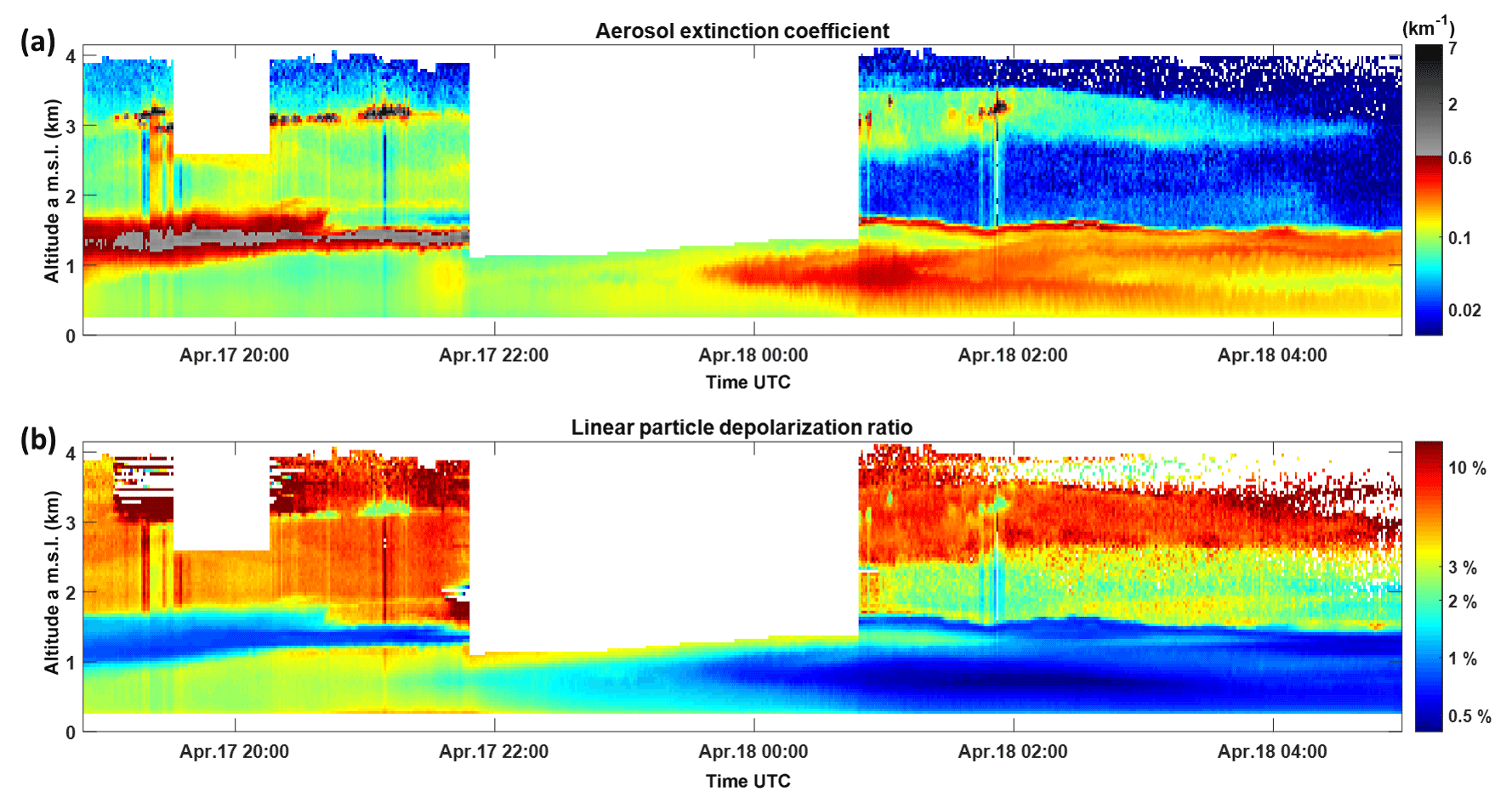
Figure 9Time series, from 17 April at 18:50 UTC to 18 April at 05:00 UTC, of the profiles of (a) aerosol extinction coefficient (AEC), and (b) linear particle depolarization ratio (PDR). The PDR is only considered for AEC > 0.01 km−1.
4.1 Lidar-derived aerosol optical properties in the low–middle troposphere
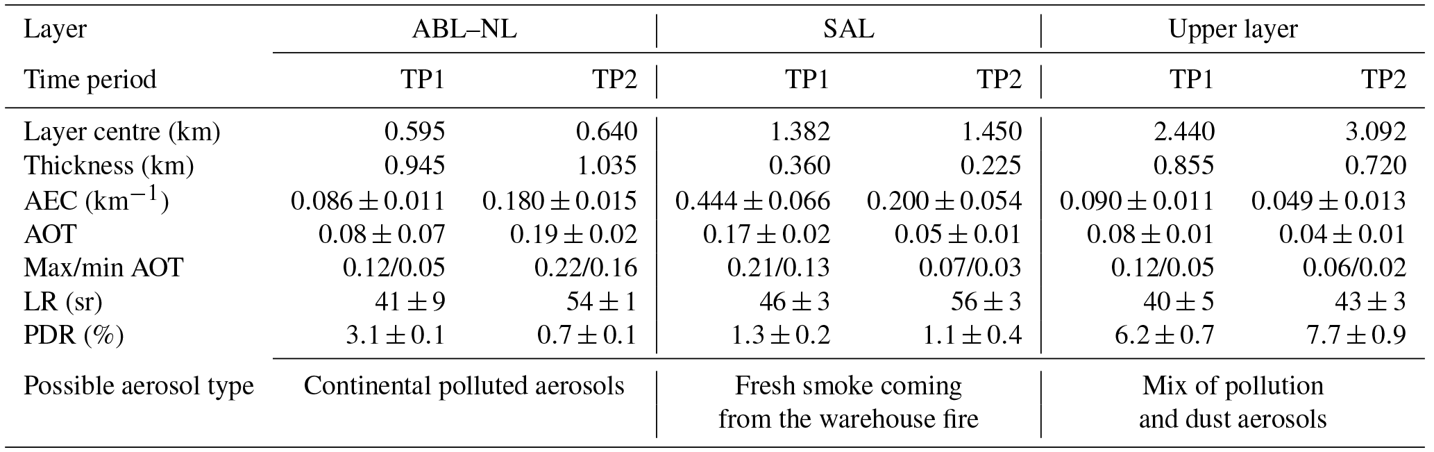
The lidar observations of the low troposphere following the accidental fire event are analysed using the TDAM approach. Lidar data are time-averaged over 60 min to increase the SNR, especially for the N2 Raman channel. The reference zone of each profile is chosen below the thick stratus cloud. The TDAM algorithm is applied to the average profiles for the whole observation period to retrieve the aerosol optical parameters and mainly the vertical profile of the LR. The LR profiles are then used to invert the 1 min resolution elastic signal to assess the vertical profile of the AEC. As previously explained, the PDR is only calculated for AEC greater than 0.01 km−1, as it is undefined and noisy for lower values. The temporal evolutions of retrieved vertical profiles of both AEC and PDR are shown in Fig. 9. Two examples of retrieved vertical profiles are also given in Fig. 10; each one is related to 60 profiles of ∼1 h acquisition time centred on 17 April at 20:49 UTC or 18 April at 01:52 UTC. The standard deviations around the mean values are represented by grey areas, showing the uncertainty due to the signal averaging during varying atmospheric extinction and scattering conditions. Two other time periods are selected, when there are no clouds in the considered layers, during which the average optical properties of three layers are summarized in Table 2.
We can easily figure out that the ABL or NL are well decoupled from the free troposphere through the intensity of the backscattered signal (Fig. 3a). Before and after 17 April at 22:00 UTC, aerosol typing in the first kilometre of the atmosphere appears different, with a significant decrease in the PDR from ∼3 % to ∼0.5 %. In both cases, the aerosols are likely spherical, as they are associated with a small depolarization ratio. This temporal evolution may be due to aerosols of different origins being advected over time. The LR in the ABL–NL is found to be between 40 and 70 sr, as usually observed in the Paris area (e.g. Royer et al., 2011).
One thin layer is located just at the top of the ABL–NL, close to 1.2 km a.m.s.l. This aerosol layer is associated with a strong AEC ( km−1) and a small PDR ( %). It is related to the fresh smoke plume coming from the accidental fire. These aerosols are non-depolarizing and therefore very likely to be spherical and composed of water-soluble compounds trapped inside their shell. The LR of the smoke plume is sr. The partial AOT of this layer ranges from 0.1 to 0.3, and dominates the AOT of the full atmospheric column.
The upper, more depolarizing aerosol layer, located between 1.8 and 3 km a.m.s.l., presents a PDR of % and a LR sr, which is characteristic of a mix of pollution and dust aerosols. This layer fades in the morning of 18 April. Within this layer, as within the smoke plume, aerosols seem to favour the formation of clouds, which results in an intense backscattered signal (the grey area seen in Fig. 3), and necessitates the presence of hydrophilic particles.
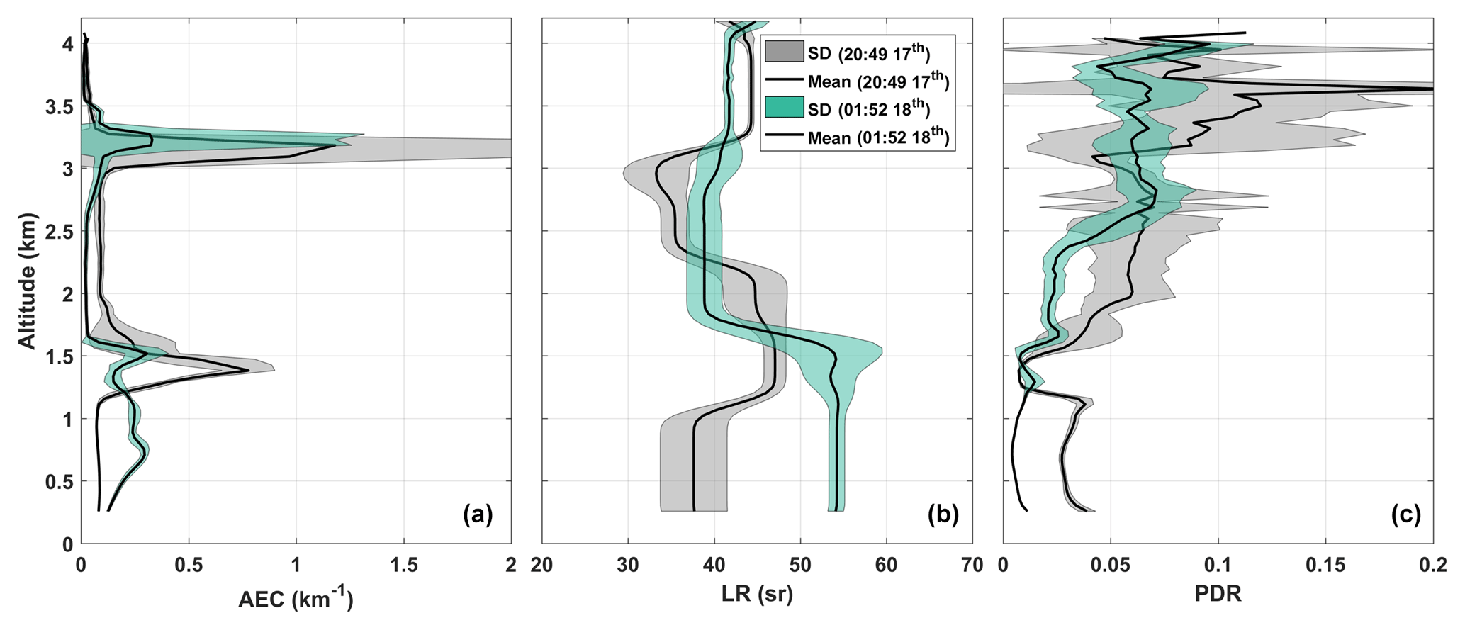
Figure 10Examples of retrieved profiles of (a) aerosol extinction coefficient (AEC), (b) lidar ratio (LR), and (c) linear particle depolarization ratio (PDR) of 1 h lidar measurements centred on 17 April 20:49 UTC and 18 April 01:52 UTC. Mean values are shown by black lines and grey and green shaded areas indicate the atmospheric variability during this 1 h period.
Table 2Average optical properties (at 355 nm) for the ABL–NL (atmospheric boundary layer–nocturnal layer), the SAL (smoke aerosol layer), and the upper layer during two time periods (TPs): TP1: 17 April, 20:19–21:35 UTC, TP2: 18 April, 02:00–04:00 UTC. The atmospheric variability during the time period is given by the standard derivation values.
4.2 Discussion
4.2.1 Comparison of the warehouse fire smoke and biomass burning smoke
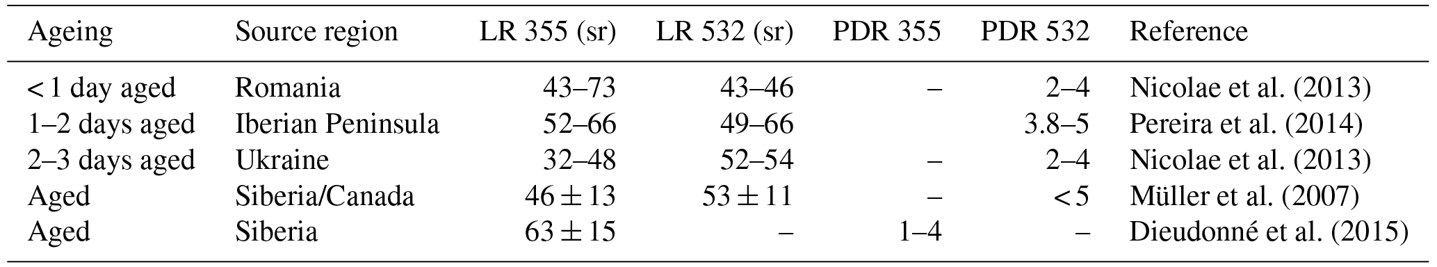
The freshly emitted smoke plumes from an accidental warehouse fire were sampled. Such observations are absent in the literature, so we compared the optical properties of SAL from the warehouse fire (in Table 2) with the ones of biomass burning smoke (Table 3). Simultaneous observations at 355 and 532 nm showed a strong wavelength dependency of the LR of aged biomass burning aerosols (Müller et al., 2007; Nicolae et al., 2013) and a smaller dependency for fresh biomass burning aerosols (Nicolae et al., 2013; Pereira et al., 2014). Our measurements will be compared preferentially with other observations at 355 nm. The LR found for SAL is in the middle range of the large dispersion of 355 nm LR values (from 32 to 73 sr) found from the literature (Table 3). Measurement of a mixed smoke and dust layer suggests that the PDR does not vary much with wavelength (Groß et al., 2011). The PDR at 355 nm of SAL (∼1 %) in this study is small compared to the PDR at 532 nm retrieved for smoke in the literature (2 %–5 %, Table 3). We reported measurement of biomass burning particles with a LR of ∼63 and a PDR of 1 %–4 % over the Siberra region (Dieudonné et al., 2015, Table 3), using a similar lidar system.
Table 3Optical properties found in the literature about biomass burning events and used to compare with the obtained values of the warehouse fire SAL (smoke aerosol layer) in Table 2.
4.2.2 Exogenous observations to confirm lidar-derived hypotheses
The total AOT and the visible Ångström exponent were extracted from the Aerosol Robotic Network (AERONET) for the sun photometer located at Palaiseau (http://aeronet.gsfc.nasa.gov/, last access: 3 December 2018; Fig. 1). Elevated AOT values, between 0.58 and 0.95 at 355 nm, were observed on 17 April. This is the peak value of the whole month (the monthly mean AOT is ∼0.2 in cloud-free conditions, corresponding to the background conditions as shown by Chazette and Royer, 2017). Nevertheless, there is only one available value (0.95) at ∼ 16:20 UTC, from 14:30 UTC to the end of the day (17 April), due to the cloud cover.
Four downwind air quality stations (AS; Fig. 1a) of the AIRPARIF air quality network (http://www.airparif.asso.fr/, last access: 3 December 2018) measured the PM10 concentrations at ∼3 m above ground level during the warehouse fire event, as shown in Fig. 1c. The one nearest AS1 is a traffic station, 4 km away from the warehouse fire location. The average daytime value at AS1 on 17 April was ∼60 µg m−3, exceeding the information threshold for air quality; two outlying values exceed the alert threshold at around 18:00 and 20:00 UTC. However, there was no significant increase in PM10 compared to the values of the whole month. The warehouse fire mainly injected aerosols into the low free troposphere by pyro-convection, just above the ABL situated close to 1 km a.m.s.l. This kind of event appears to have a negligible impact on the air quality measured at ground level. It mainly impacts the lower free troposphere, just above the ABL, as shown from lidar measurements.
In Sect. 4.1, we found that lidar-derived optical parameters are quite different for aerosols in the ABL–NL before and after 17 April at 22:00 UTC. It should be due to the change in air mass. In order to investigate the origins of these aerosols, back-trajectory analysis in ensemble mode was performed using the NOAA HYSPLIT model (HYbrid Single-Particle Lagrangian Integrated Trajectory model, available at http://ready.arl.noaa.gov, last access: 3 December 2018). Results show that for the first part (before 22:00 UTC in Fig. 9), air mass origin is mainly from the south of France with a mix from the west of Germany, whereas for the second part (after 22:00 UTC in Fig. 9), air masses seem to be only coming from Benelux and Germany, loaded with pollution particles. Note that it was raining during the night from 16 to 17 April, and there was no rain during the day of 17 April (http://sirta.ipsl.fr/, last access: 3 December 2018).
The origin of the upper depolarized aerosol plume, located between 1.8 and 3 km a.m.s.l. (Fig. 9), was also investigated. The reanalysed products of the numerical weather prediction model ECMWF IFS (http://www.ecmwf.int, last access: 3 December 2018) are used to provide the meteorological fields. The one at 750 hPa (∼2.5 km a.m.s.l.) on 16 April 00:00 UTC shows that a corridor has been created between northern Africa and western Europe, which favoured the transport of dusts, associated with a low located on the Iberian Peninsula backed by a ridge joining the Sahara to western Europe (Fig. S1 in the Supplement). The low attenuated when it moved eastward. Another more active low was enhanced near the Coruña region (Fig. S1). The latter allowed a recirculation of air masses, initially loaded with dust, above the UK and then towards France. The AOT at 550 nm from daily MODIS level 2 aerosol products (MYD04_L2 and MOD04_L2) also shows the transport of dusts from Morocco and Algeria to France on 16 April (Fig. S2). Note that in the area around Paris, the MODIS-derived AOT is on 17 April, matching the in situ measurements. These air masses moved eastward on 17 April and did not contribute directly to dust loads over the Paris area. The dust plume seen on the lidar measurements is probably related to the recirculation of air masses on 16 April. This plume is easily identified (Fig. S3) as dust layers between 2 and 4 km a.m.s.l. over the English Channel on the lidar vertical feature mask data product (Level 2, v4.10; Burton et al., 2013) derived from the CALIOP (Cloud-Aerosol Lidar with Orthogonal Polarization, https://www-calipso.larc.nasa.gov/, last access: 3 December 2018) measurements. The CALIOP-derived PDR at 532 nm of this dust layer has values of the order of 30 % (the related PDR at 355 nm is ∼25 % as proposed in Groß et al., 2015) corresponding to dust aerosols. The 6-day back trajectories (Fig. S3) illustrate that for the aerosol plume examined between 1.8 and 3 km a.m.s.l. over the Paris area, a very strong recirculation can be observed on 17 April at 18:00 UTC. The contribution originating directly from northern Africa is very weak.
For the first time, a ground-based N2 Raman lidar sampled freshly emitted smoke plumes originating from a large accidental warehouse fire that occurred on 17 April 2015. It was an exceptional event for the Paris area, but despite a strong smell throughout the region, it did not significantly exceed background aerosol levels measured by the ground-based air quality network before it was observed by the automatic N2 Raman LAASURS located 15 km south of Paris. The lidar profiles have been inverted using a new algorithm named top-down aerosol optical thickness matching (TDAM). Such an approach allows for the retrieval of the aerosol extinction and backscatter coefficients and lidar ratio in complex cases with a highly inhomogeneous atmosphere. Furthermore, this method can be used in the event of a limited maximum range or a thick aerosol load that prevents a purely molecular zone for normalization being prevented, as required by traditional methods. The uncertainties of the TDAM inversion are studied, showing good accuracy in the retrieved aerosol optical parameters: e.g. for the observed warehouse fire smoke aerosol layer, the uncertainties are 10 sr for the lidar ratio, 0.1 km−1 for the AEC, and 0.1 % for the PDR. Overall, the TDAM approach proves advantageous in heterogeneous atmospheric conditions, with a better effective vertical resolution and less bias when there are aerosols in the free troposphere.
The optical properties of the warehouse fire smoke aerosols were characterized using this TDAM approach. This thin smoke plume, ∼ 0.4 km wide, located at ∼1.2 km a.m.s.l., has a strong AEC (∼ 0.8 km−1) and a small PDR (∼1 %), containing spherical, moderately absorbent aerosols. The LR of the fire smoke plume was derived as ∼50 sr at 355 nm wavelength and corresponds to values previously retrieved for polluted dust aerosol or long-range-transported biomass burning aerosols.
The Raman lidar system is shown once again to be a strong tool to sample aerosol layers during extreme events, which argues for the existence of lidar networks dedicated to the monitoring of air quality and airborne threats due to exceptional events that can occur in urban areas.
All data are available from the authors upon request.
The supplement related to this article is available online at: https://doi.org/10.5194/amt-11-6525-2018-supplement.
XS participated in the experiment, analysed the Raman lidar data, developed the algorithm, and wrote the paper; PC conceived and managed the project, performed the experiment, developed the algorithm, and participated in the editing of the paper; JT maintained the Raman lidar and participated in the experiment and the editing of the paper.
The authors declare that they have no conflict of interest.
This work was supported by the Commissariat à l'Energie Atomique et aux
énergies alternatives (CEA). The authors would like to thank the
AIRPARIF network for providing ground-level aerosol data (available at
http://www.airparif.asso.fr/en/telechargement/telechargement-station, last access: 3 December 2018) and the
AERONET network for sun photometer products (at
https://aeronet.gsfc.nasa.gov/, last access: 3 December 2018). The authors acknowledge the MODIS Science,
Processing and Data Support Teams for producing and providing MODIS data (at
https://modis.gsfc.nasa.gov/data/dataprod/, last access: 3 December 2018), and the NASA Langley Research
Center Atmospheric Sciences Data Center for the data processing and
distribution of CALIPSO products (level 4.10, at
https://eosweb.larc.nasa.gov/HORDERBIN/HTML_Start.cgi, last access: 3 December 2018). The
NOAA Air Resources Laboratory (ARL) is acknowledged for the provision of the
HYSPLIT transport and dispersion model and READY website
(http://www.ready.noaa.gov, last access: 3 December 2018) used in this publication. ECMWF data used in
this study were obtained from the ESPRI/IPSL data server.
Edited by: Ulla Wandinger
Reviewed by: two anonymous referees
Ångström, A.: The parameters of atmospheric turbidity, Tellus A, 16, 64–75, https://doi.org/10.3402/tellusa.v16i1.8885, 1964.
Ansmann, A.: Ground-truth aerosol lidar observations: can the Klett solutions obtained from ground and space be equal for the same aerosol case?, Appl. Opt., 45, 3367, https://doi.org/10.1364/AO.45.003367, 2006.
Ansmann, A., Riebesell, M., and Weitkamp, C.: Measurement of atmospheric aerosol extinction profiles with a Raman lidar, Opt. Lett., 15, 746, https://doi.org/10.1364/OL.15.000746, 1990.
Ansmann, A., Wandinger, U., Riebesell, M., Weitkamp, C., and Michaelis, W.: Independent measurement of extinction and backscatter profiles in cirrus clouds by using a combined Raman elastic-backscatter lidar., Appl. Opt., 31, 7113, https://doi.org/10.1364/AO.31.007113, 1992.
Ansmann, A., Seifert, P., Tesche, M., and Wandinger, U.: Profiling of fine and coarse particle mass: case studies of Saharan dust and Eyjafjallajökull/Grimsvötn volcanic plumes, Atmos. Chem. Phys., 12, 9399–9415, https://doi.org/10.5194/acp-12-9399-2012, 2012.
Behrendt, A., Wulfmeyer, V., Schaberl, T., Bauer, H.-S., Kiemle, C., Ehret, G., Flamant, C., Kooi, S., Ismail, S., Ferrare, R., Browell, E. V., and Whiteman, D. N.: Intercomparison of Water Vapor Data Measured with Lidar during IHOP_2002, Part II: Airborne-to-Airborne Systems, J. Atmos. Ocean. Technol., 24, 22–39, https://doi.org/10.1175/JTECH1925.1, 2007.
Binietoglou, I., Basart, S., Alados-Arboledas, L., Amiridis, V., Argyrouli, A., Baars, H., Baldasano, J. M., Balis, D., Belegante, L., Bravo-Aranda, J. A., Burlizzi, P., Carrasco, V., Chaikovsky, A., Comerón, A., D'Amico, G., Filioglou, M., Granados-Muñoz, M. J., Guerrero-Rascado, J. L., Ilic, L., Kokkalis, P., Maurizi, A., Mona, L., Monti, F., Muñoz-Porcar, C., Nicolae, D., Papayannis, A., Pappalardo, G., Pejanovic, G., Pereira, S. N., Perrone, M. R., Pietruczuk, A., Posyniak, M., Rocadenbosch, F., Rodríguez-Gómez, A., Sicard, M., Siomos, N., Szkop, A., Terradellas, E., Tsekeri, A., Vukovic, A., Wandinger, U., and Wagner, J.: A methodology for investigating dust model performance using synergistic EARLINET/AERONET dust concentration retrievals, Atmos. Meas. Tech., 8, 3577–3600, https://doi.org/10.5194/amt-8-3577-2015, 2015.
Burton, S. P., Ferrare, R. A., Vaughan, M. A., Omar, A. H., Rogers, R. R., Hostetler, C. A., and Hair, J. W.: Aerosol classification from airborne HSRL and comparisons with the CALIPSO vertical feature mask, Atmos. Meas. Tech., 6, 1397–1412, https://doi.org/10.5194/amt-6-1397-2013, 2013.
Chazette, P. and Royer, P.: Springtime major pollution events by aerosol over Paris Area: From a case study to a multiannual analysis, J. Geophys. Res.-Atmos., 122, 8101–8119, https://doi.org/10.1002/2017JD026713, 2017.
Chazette, P., Pelon, J., and Mégie, G.: Determination by spaceborne backscatter lidar of the structural parameters of atmospheric scattering layers., Appl. Opt., 40, 3428–3440, 2001.
Chazette, P., Sanak, J., and Dulac, F.: New approach for aerosol profiling with a lidar onboard an ultralight aircraft: application to the African Monsoon Multidisciplinary Analysis., Environ. Sci. Technol., 41, 8335–8341, https://doi.org/10.1021/es070343y, 2007.
Chazette, P., Raut, J.-C., Dulac, F., Berthier, S., Kim, S.-W., Royer, P., Sanak, J., Loaëc, S., and Grigaut-Desbrosses, H.: Simultaneous observations of lower tropospheric continental aerosols with a ground-based, an airborne, and the spaceborne CALIOP lidar system, J. Geophys. Res., 115, D00H31, https://doi.org/10.1029/2009JD012341, 2010.
Chazette, P., Dabas, A., Sanak, J., Lardier, M., and Royer, P.: French airborne lidar measurements for Eyjafjallajökull ash plume survey, Atmos. Chem. Phys., 12, 7059–7072, https://doi.org/10.5194/acp-12-7059-2012, 2012.
Chazette, P., Marnas, F., and Totems, J.: The mobile Water vapor Aerosol Raman LIdar and its implication in the framework of the HyMeX and ChArMEx programs: application to a dust transport process, Atmos. Meas. Tech., 7, 1629–1647, https://doi.org/10.5194/amt-7-1629-2014, 2014.
Chazette, P., Totems, J., Ancellet, G., Pelon, J., and Sicard, M.: Temporal consistency of lidar observations during aerosol transport events in the framework of the ChArMEx/ADRIMED campaign at Minorca in June 2013, Atmos. Chem. Phys., 16, 2863–2875, https://doi.org/10.5194/acp-16-2863-2016, 2016.
Collis, R. T. H. and Russel, P. B.: Laser Monitoring of the Atmosphere, edited by: Hinkley, E. D., Springer Berlin Heidelberg, Berlin, Heidelberg, 1976.
Dieudonné, E., Chazette, P., Marnas, F., Totems, J., and Shang, X.: Lidar profiling of aerosol optical properties from Paris to Lake Baikal (Siberia), Atmos. Chem. Phys., 15, 5007–5026, https://doi.org/10.5194/acp-15-5007-2015, 2015.
Di Girolamo, P.: Rotational Raman Lidar measurements of atmospheric temperature in the UV, Geophys. Res. Lett., 31, L01106, https://doi.org/10.1029/2003GL018342, 2004.
Dubovik, O., Holben, B., Eck, T. F., Smirnov, A., Kaufman, Y. J., King, M. D., Tanré, D., and Slutsker, I.: Variability of Absorption and Optical Properties of Key Aerosol Types Observed in Worldwide Locations, J. Atmos. Sci., 59, 590–608, https://doi.org/10.1175/1520-0469(2002)059<0590:VOAAOP>2.0.CO;2, 2002.
Groß, S., Gasteiger, J., Freudenthaler, V., Wiegner, M., Geiß, A., Schladitz, A., Toledano, C., Kandler, K., Tesche, M., Ansmann, A., and Wiedensohler, A.: Characterization of the planetary boundary layer during SAMUM-2 by means of lidar measurements, Tellus B., 63, 695–705, https://doi.org/10.1111/j.1600-0889.2011.00557.x, 2011.
Groß, S., Freudenthaler, V., Schepanski, K., Toledano, C., Schäfler, A., Ansmann, A., and Weinzierl, B.: Optical properties of long-range transported Saharan dust over Barbados as measured by dual-wavelength depolarization Raman lidar measurements, Atmos. Chem. Phys., 15, 11067–11080, https://doi.org/10.5194/acp-15-11067-2015, 2015.
Haustein, K., Pérez, C., Baldasano, J. M., Müller, D., Tesche, M., Schladitz, A., Esselborn, M., Weinzierl, B., Kandler, K., and von Hoyningen-Huene, W.: Regional dust model performance during SAMUM 2006, Geophys. Res. Lett., 36, L03812, https://doi.org/10.1029/2008GL036463, 2009.
Kanitz, T., Ansmann, A., Seifert, P., Engelmann, R., Kalisch, J., and Althausen, D.: Radiative effect of aerosols above the northern and southern Atlantic Ocean as determined from shipborne lidar observations, J. Geophys. Res. Atmos., 118, 12556–12565, https://doi.org/10.1002/2013JD019750, 2013.
King, L. V.: On the Complex Anisotropic Molecule in Relation to the Dispersion and Scattering of Light, Proc. Royal Soc. London, 1, 333–357 available at: http://www.researchgate.net/publication/247031191_On_the_Complex_Anisotropic_Molecule_in_Relation_to_the_Dispersion_and_Scattering_of_Light (last access: 30 July 2014), 1923.
Klett, J. D.: Stable analytical inversion solution for processing lidar returns, Appl. Opt., 20, 211, https://doi.org/10.1364/AO.20.000211, 1981.
Mattis, I., Siefert, P., Müller, D., Tesche, M., Hiebsch, A., Kanitz, T., Schmidt, J., Finger, F., Wandinger, U., and Ansmann, A.: Volcanic aerosol layers observed with multiwavelength Raman lidar over central Europe in 2008–2009, J. Geophys. Res., 115, D00L04, https://doi.org/10.1029/2009JD013472, 2010.
Measures, R. M.: Laser Remote Sensing: Fundamentals and Applications, edited by: Wiley, J., Krieger publishing company, Malabar, Florida, USA, 1984.
Müller, D., Ansmann, A., Mattis, I., Tesche, M., Wandinger, U., Althausen, D., and Pisani, G.: Aerosol-type-dependent lidar ratios observed with Raman lidar, J. Geophys. Res., 112, D16202, https://doi.org/10.1029/2006JD008292, 2007.
Nicolae, D., Nemuc, A., Müller, D., Talianu, C., Vasilescu, J., Belegante, L., and Kolgotin, A.: Characterization of fresh and aged biomass burning events using multiwavelength Raman lidar and mass spectrometry, J. Geophys. Res.-Atmos., 118, 2956–2965, https://doi.org/10.1002/jgrd.50324, 2013.
Nicolet, M.: On the molecular scattering in the terrestrial atmosphere?: An empirical formula for its calculation in the homosphere, Planet. Space Sci., 32, 1467–1468, https://doi.org/10.1016/0032-0633(84)90089-8, 1984.
Pappalardo, G., Amodeo, A., Pandolfi, M., Wandinger, U., Ansmann, A., Bösenberg, J., Matthias, V., Amiridis, V., De Tomasi, F., Frioud, M., Iarlori, M., Komguem, L., Papayannis, A., Rocadenbosch, F., and Wang, X.: Aerosol lidar intercomparison in the framework of the EARLINET project 3 Raman lidar algorithm for aerosol extinction, backscatter, and lidar ratio, Appl. Opt., 43, 5370, https://doi.org/10.1364/AO.43.005370, 2004.
Pereira, S. N., Preißler, J., Guerrero-Rascado, J. L., Silva, A. M., and Wagner, F.: Forest fire smoke layers observed in the free troposphere over Portugal with a multiwavelength Raman lidar: optical and microphysical properties., Sci. World J., 2014, 421838, https://doi.org/10.1155/2014/421838, 2014.
Royer, P., Chazette, P., Lardier, M., and Sauvage, L.: Aerosol content survey by mini N2-Raman lidar: Application to local and long-range transport aerosols, Atmos. Environ., 45, 7487–7495, https://doi.org/10.1016/j.atmosenv.2010.11.001, 2011.
Sasano, Y., Browell, E. V., and Ismail, S.: Error caused by using a constant extinction/backscattering ratio in the lidar solution, Appl. Opt., 24, 3929, https://doi.org/10.1364/AO.24.003929, 1985.
Shang, X. and Chazette, P.: End-to-End Simulation for a Forest-Dedicated Full-Waveform Lidar Onboard a Satellite Initialized from Airborne Ultraviolet Lidar Experiments, Remote Sens., 7, 5222–5255, https://doi.org/10.3390/rs70505222, 2015.
Shcherbakov, V.: Regularized algorithm for Raman lidar data processing, Appl. Opt., 46, 4879, https://doi.org/10.1364/AO.46.004879, 2007.
Tikhonov, A. N. and Arsenin, V. Y.: Solutions of Ill-Posed Problems, Math. Comput., 32, 1320–1322, 1978.
Wang, Y., Sartelet, K. N., Bocquet, M., and Chazette, P.: Modelling and assimilation of lidar signals over Greater Paris during the MEGAPOLI summer campaign, Atmos. Chem. Phys., 14, 3511–3532, https://doi.org/10.5194/acp-14-3511-2014, 2014.
Weitkamp, C.: Lidar?: range-resolved optical remote sensing of the atmosphere, Springer, New York, 2005.
Whiteman, D. N.: Application of statistical methods to the determination of slope in lidar data, Appl. Opt., 38, 3360, https://doi.org/10.1364/AO.38.003360, 1999.
Whiteman, D. N.: Examination of the traditional Raman lidar technique I Evaluating the temperature-dependent lidar equations, Appl. Opt., 42, 2571, https://doi.org/10.1364/AO.42.002571, 2003.
Whiteman, D. N., Melfi, S. H., and Ferrare, R. A.: Raman lidar system for the measurement of water vapor and aerosols in the Earth's atmosphere., Appl. Opt., 31, 3068–3082, https://doi.org/10.1364/AO.31.003068, 1992.