the Creative Commons Attribution 4.0 License.
the Creative Commons Attribution 4.0 License.
 | 19 Dec 2018
A fully autonomous ozone, aerosol and nighttime water vapor lidar: a synergistic approach to profiling the atmosphere in the Canadian oil sands region
Kevin B. Strawbridge
Michael S. Travis
Bernard J. Firanski
Jeffrey R. Brook
Ralf Staebler
Thierry Leblanc
Lidar technology has been rapidly advancing over the past several decades. It can be used to measure a variety of atmospheric constituents at very high temporal and spatial resolutions. While the number of lidars continues to increase worldwide, there is generally a dependency on an operator, particularly for high-powered lidar systems. Environment and Climate Change Canada (ECCC) has recently developed a fully autonomous, mobile lidar system called AMOLITE (Autonomous Mobile Ozone Lidar Instrument for Tropospheric Experiments) to simultaneously measure the vertical profile of tropospheric ozone, aerosol and water vapor (nighttime only) from near the ground to altitudes reaching 10 to 15 km. This current system uses a dual-laser, dual-lidar design housed in a single climate-controlled trailer. Ozone profiles are measured by the differential absorption lidar (DIAL) technique using a single 1 m Raman cell filled with CO2. The DIAL wavelengths of 287 and 299 nm are generated as the second and third Stokes lines resulting from stimulated Raman scattering of the cell pumped using the fourth harmonic of a Nd:YAG laser (266 nm). The aerosol lidar transmits three wavelengths simultaneously (355, 532 and 1064 nm) employing a detector designed to measure the three backscatter channels, two nitrogen Raman channels (387 and 607 nm) and one cross-polarization channel at 355 nm. In addition, we added a water vapor channel arising from the Raman-shifted 355 nm output (407 nm) to provide nighttime water vapor profiles. AMOLITE participated in a validation experiment alongside four other ozone DIAL systems before being deployed to the ECCC Oski-ôtin ground site in the Alberta oil sands region in November 2016. Ozone was found to increase throughout the troposphere by as much as a factor of 2 from stratospheric intrusions. The dry stratospheric air within the intrusion was measured to be less than 0.2 g kg−1. A biomass burning event that impacted the region over an 8-day period produced lidar ratios of 35 to 65 sr at 355 nm and 40 to 100 sr at 532. Over the same period the Ångström exponent decreased from 1.56±0.2 to 1.35±0.2 in the 2–4 km smoke region.
- Article
(11962 KB) - Full-text XML
- BibTeX
- EndNote


Tropospheric ozone, aerosols and water vapor are important atmospheric constituents affecting air quality and climate. Ozone is a short-lived climate pollutant (SLCP) and air pollutant that can have detrimental impacts on human health (Malley et al., 2015; Lippmann, 1991), agriculture (McKee, 1994) and ecosystems (Ashmore, 2005) when present at high enough concentrations. Tropospheric ozone is photo-chemically produced primarily from nitrogen oxides and volatile organic compounds (VOCs) from anthropogenic sources, is biogenically produced from forest fires (Aggarwal et al., 2018; Trickl et al., 2015) and can be enhanced through stratospheric/tropospheric transport (STT) events (Ancellet et al., 1991; Langford et al., 1996; Leblanc et al., 2011; Stohl and Trickl, 1999). Both of these latter sources can have significant impacts on ozone concentration although typically their impacts vary within the vertical distribution of the troposphere. The advantage of ozone differential absorption lidar (DIAL) is the ability to measure this vertical column with high enough temporal resolution to understand atmospheric mixing and exchange processes. Along with ozone, the vertical distribution of aerosols and water vapor can also vary considerably throughout the troposphere.
Aerosols or particulate matter are tiny particles suspended in the air which contribute to the radiative budget; are a tracer for pollution transport; and impact visibility, cloud formation and air quality. They affect the earth's climate by interacting with the sun and earth's radiation (Ramanathan et al., 2001) and by modifying clouds (Feingold et al., 2003; Twomey, 1977) and, depending on their size and the meteorological conditions, can travel over great distances around the globe (Uno et al., 2009). In high enough concentrations these particles can have dramatic effects on visibility (Li et al., 2016; Singh et al., 2017) and cause respiratory problems, particularly in those suffering from lung conditions such as asthma. This has been the motivation for several countries to adopt an air quality index (Kousha and Valacchi, 2015) to alert the public to respiratory dangers during pollution events. Aerosol backscatter lidar systems are uniquely capable of providing the vertical profile of tropospheric aerosols at very high temporal and spatial resolutions and are therefore ideal instruments to study the transport and optical properties of aerosols. While the vertical distribution of ozone and aerosols can be highly variable throughout the troposphere, water vapor tends to have the highest concentration closest to the surface and throughout the mixed layer.
Water vapor plays a pivotal role in climate change and atmospheric stability by directly influencing many atmospheric processes such as cloud formation (Pruppacher and Klett, 1997) and photochemical atmospheric reactions (Yamamoto et al., 1966; Grant, 1991). Furthermore, tropospheric water vapor is a catalyst to many atmospheric chemical reactions by functioning as a solvent for chemical products of natural and anthropogenic activities (Grant, 1991). Also, as the primary greenhouse gas, with strong infrared absorption in the 100–600 cm−1 spectral region, water vapor helps to maintain the earth's radiation balance by absorbing and emitting infrared radiation (Twomey, 1991; Clough et al., 1992; Sinha and Harries, 1995). The high spatial and temporal variability of water vapor throughout the atmosphere makes it an ideal candidate for lidar measurements (Vogelmann et al., 2015).
The purpose of this paper is to describe a vertical profile measurement system that measures ozone, aerosols and water vapor simultaneously. By employing three different lidar techniques – Mie backscatter lidar, water vapor Raman lidar and ozone DIAL – in one observation platform, we are able to explore a synergistic approach to advance our understanding of the trace gas distribution in the lower atmosphere with the eventual goal of supporting development to improve air quality forecasts, diagnostic models and satellite measurements. There are only a few sites that currently exist where all three lidar techniques are operated: Garmisch-Partenkirchen (Trickl et al., 2015), Maïdo observatory on Reunion Island (Baray et al., 2013) and Observatoire de Haute-Provence (OHP) (Bock et al., 2013; Khaykin et al., 2017; Gaudel et al., 2015). Several of these sites are high-altitude sites that began as stratospheric observatories.
The accomplishment here was to develop such a platform to be mobile and to run autonomously, providing near-continuous observations (except during precipitation events), even in remote areas. Environment and Climate Change Canada (ECCC) has designed and built a fully autonomous, mobile lidar system, based on the backbone of an earlier system design (Strawbridge, 2013) named AMOLITE (Autonomous Mobile Ozone Lidar Instrument for Tropospheric Experiments) to measure the vertical profile of tropospheric ozone, aerosol and water vapor simultaneously. To verify the system's performance, AMOLITE participated in a validation campaign known as the Southern California Ozone Observation Project (SCOOP) at the Jet Propulsion Laboratory's Table Mountain Facility in Wrightwood, CA, during August 2016. This study brought together five of the six tropospheric ozone lidars that form the Tropospheric Ozone Lidar Network – TOLNet (http://www-air.larc.nasa.gov/missions/TOLNet/, last access: 14 November 2018). In addition to the five lidars, ozone sonde balloons were launched throughout the study period. This campaign provided an excellent opportunity to evaluate the ozone profiles produced by AMOLITE. For details of the intercomparison refer to a separate publication (manuscript in preparation). Lidar networks (http://ndacc-lidar.org, last access: 14 November 2018; http://mplnet.gsfc.nasa.gov, last access: 14 November 2018; Papayannis et al., 2008; Sugimoto and Uno, 2009) are very important scientific tools that allow the collective benefit of increased geographical coverage (Langford et al., 2018; Trickl et al., 2016) and can often provide valuable climatological data (Granados-Muñoz and Leblanc, 2016; Khaykin et al., 2017; Gaudel et al., 2015). The existence of networks like TOLNet will help to address the need for more ozone profilers in the troposphere as reported in the recent Tropospheric Ozone Assessment Report (TOAR) by Gaudel et al. (2018).
After the validation campaign, AMOLITE was shipped back to Canada, where it was made ready for deployment to the oil sands region. The first AMOLITE ozone and water vapor profiles at the Oski-ôtin ground site in Fort McKay, Alberta, were acquired on 3 November 2016. In addition to the lidar measurements, operation of a windRASS (wind radio-acoustic sounding system – model MFAS, Scintec, Rottenburg, Germany) provides the local meteorological wind fields at 10 m vertical resolution from 40 to typically 500 m above ground, directly determining the upwind sources near ground level and aloft over the site. These remote sensors provide a coherent 3-D picture of the transport processes impacting the ground site and the region nearby. Also housed in a trailer on site is a chemistry observing platform called Comprehensive Air Monitoring # 1 (CAM1) that has an extensive suite of ground-based instrumentation that continuously measures a variety of gaseous and particulate pollutants. The purpose of this site is to identify the predominant sources impacting the region and the main local-scale atmospheric processes influencing pollutant transport, transformation and deposition. This information will be used to improve our knowledge of what is being emitted and the processes in the atmosphere that affect where the pollutants move and deposit.
The focus of this paper will be on the additional development required to add the ozone and water vapor capability to the previous autonomous aerosol lidar design developed by ECCC, followed by a brief section on the validation and verification of the instrument and processing algorithms. The fourth section will describe a few case studies acquired throughout the first year of operation at the Oski-ôtin ground site in Fort McKay. The final section will draw conclusions and discuss some future improvements that are currently underway for AMOLITE.
The AMOLITE instrument uses three different lidar techniques to measure different atmospheric constituents: a Mie backscatter lidar to measure the vertical profile of aerosol at three different wavelengths, a DIAL to measure the vertical ozone profile and a Raman lidar to measure the water vapor profile. The Mie backscatter aerosol lidar technique used in AMOLITE has already been described in detail by Strawbridge (2013). Here we briefly describe the DIAL and Raman lidar techniques used for the systems in AMOLITE.
2.1 Ozone DIAL technique
Using the DIAL technique, it is possible to retrieve ozone mixing ratios from the backscatter profiles. The technique essentially uses the differential absorption of ozone at two different wavelengths that are relatively close together to minimize aerosol effects but far enough apart to have a sufficiently large difference in their ozone absorption cross sections. Consequently, the ozone calculation uses the two-wavelength solution of the lidar equation given below (Kovalev and McElroy, 1994):
where αon−αoff is the differential ozone absorption cross section, is the signal ratio, is the ratio of the backscatter coefficient at the “on” and “off” wavelengths and 2Δσ(z) is the total two-way extinction coefficient differential, Δαi is the differential cross section of the interfering trace gas and ni(z) is the number density profile of the interfering trace gas. In our system, 287 nm represents the on wavelength, and 299 nm represents the off wavelength. It is possible to express the backscatter contribution overall to the ozone calculation at the on and off wavelengths based solely on the ratio between the aerosol and molecular backscatter,B∗(z), at some reference wavelength. This is represented by
where υ is the Ångström exponent representing the wavelength dependence of aerosol Mie backscatter and in our case the reference wavelength is 355 nm. The difficulty arises in determining the Ångström exponent in regions where the aerosol concentrations are lower and with enough precision to provide an accurate correction. This point is illustrated for a forest fire case shown in Sect. 4.3. In addition, the Ångström exponent determined by our system reflects the wavelength dependence of aerosol backscatter between 355 and 532 nm, which may be different than the wavelength dependence between the on- and offline wavelengths of 287 and 299 nm.
2.2 Water vapor Raman technique
During the early stages of the optical detector design for the aerosol lidar, it was determined that with the addition of a few optics (see Fig. 2), which requires very little additional space in the detector design, it would be possible to measure nighttime water vapor using the Raman technique on the 355 nm laser wavelength. This would be particularly valuable when identifying STT events where the dry stratospheric air can be easily identified by the water vapor lidar measurements. Raman scattering is an inelastic quantum-mechanical scattering process, in which the wavelength of the incident radiation is shifted as a result of the interaction of the photons with target molecules. The Raman wavelength shift, related to the exciting laser wavelength (λL), is proportional to the distinct ro-vibrational energy levels and provides a unique fingerprint for each molecule. The Raman scattering process can involve either energy absorption by the molecule, producing Stokes Raman scattered light with less energy (longer wavelength), or energy transferred to the molecule, producing anti-Stokes Raman scattered light with more energy (shorter wavelength). Most atmospheric species are vibrationally active – resulting in a net Raman shift to longer wavelengths (λr>λL), which indicates that atmospheric target molecules gain energy from the radiation field. The most probable Raman shifts for N2 and H2O are at 2330.7 and 3652.0 cm−1, respectively (Whiteman et al., 1992).
The ratio between the water vapor and nitrogen Raman signals yields a mathematical expression for the dependence of Raman signals ratio on water vapor and nitrogen molecular density ( and ), namely
where R is the proportionality constant dependent on the instrument specifications. This equation ignores the temperature-dependent functions required for very narrow bandwidth filters, typically used for daytime operation (see Whiteman, 2003).
The water vapor mixing ratio (WVMR, denoted as w(z), in grams of water vapor per kilogram of dry air) as a function of vertical altitude (z) is proportional to the ratio of the number density of water vapor to nitrogen and is given by (Goldsmith et al., 1998)
The WVMR equation above can be related to experimentally recorded Raman lidar signals, SG, by comparing Eqs. (3) and (4), leading to the following expression:
where D (in grams per kilogram) is a constant depending on instrumental specifications, ratio between N2 and H2O backscattering cross sections, N2 mixing ratio, and Raman lidar signals extinction due to the aerosols and air molecules (Dionisi et al., 2009). The D constant is commonly evaluated by comparison with independent measurement (radiosonde) of water vapor mixing ratio (w(z)).
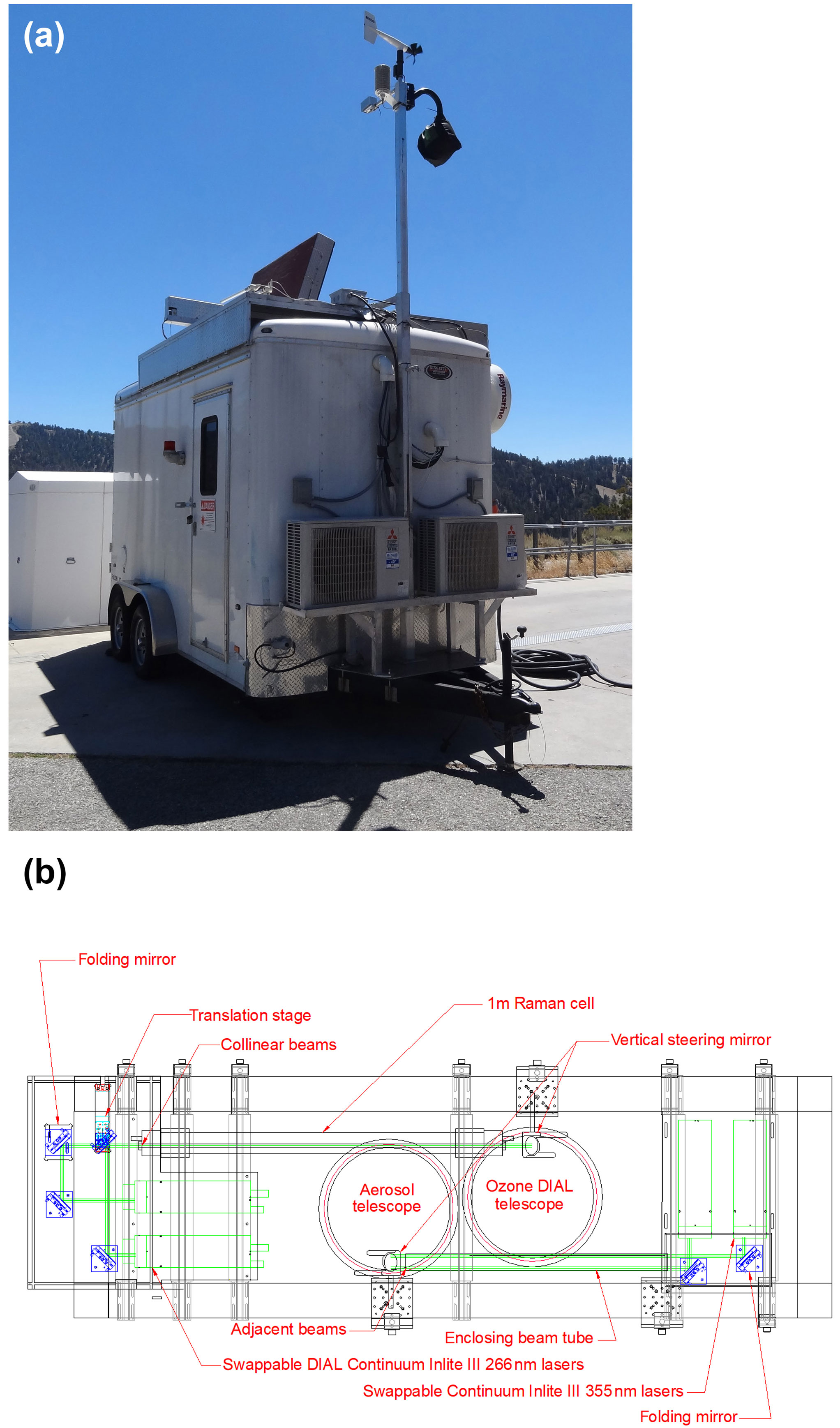
Figure 1(a) A picture showing AMOLITE on location during the SCOOP campaign at Table Mountain in California. (b) A schematic diagram of the dual-laser, dual-lidar design of AMOLITE. Both lidar systems are mounted on the same optical bench.
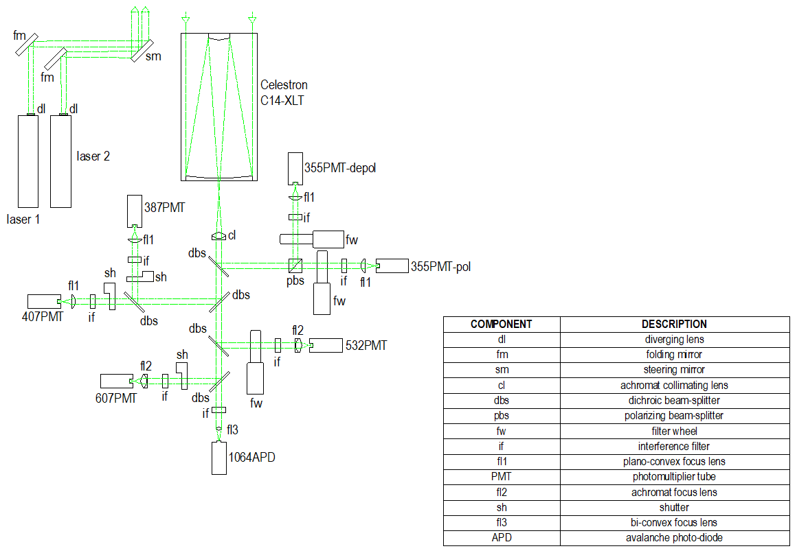
Figure 2A schematic showing the transmitter and receiver of the aerosol and water vapor lidar. A detailed optical breakout is shown for the seven-channel detector package. The abbreviations are explained in a separate box in the figure.
3.1 Trailer design and infrastructure
The current system described here builds upon the successes of the autonomous aerosol lidars built over the past decade by ECCC (Strawbridge, 2013). AMOLITE uses a synergistic approach which combines a dual-laser (for redundancy), dual-lidar design (tropospheric ozone DIAL and aerosol lidar) housed in the same trailer. In order to accommodate two lidar systems, the trailer needed to have a slightly larger interior footprint of 2.1 m by 4.3 m long. A picture of AMOLITE, operating in fully autonomous mode, deployed on a field experiment is shown in Fig. 1a. The external infrastructure of the trailer was very similar to previous designs utilizing a meteorological tower, precipitation-sensor-enabled hatch cover, modified vertically pointing radar interlock system and the other safety equipment required for operation of a class IV laser. The main differences in the design were the addition of a second radome to provide safety radar redundancy, larger hatch opening to allow the operation of two lidar receivers simultaneously and a greatly improved heating and cooling system. The second radar system allows one to remotely change between radar sources in the event that a system failure occurs. We found that these radomes would typically last between 2 and 4 years. However, when a failure occurs, the lidar system is shut down for safety reasons until a site visit can be arranged and a new radar system installed. The addition of a second radar reduced system downtime and operational costs. The larger hatch not only is necessary for dual-lidar operation, but it was also modified to allow the wiper system to operate while the hatch is either open or closed. It was also designed to accommodate exterior blower fans to prevent the accumulation of insects on the window attracted by the UV laser light. The most significant upgrade was the addition of two Mitsubishi Mr. Slim ducted units capable of delivering between 6000 and 24 000 BTU of cooling as well as heat units mounted in the duct allowing an operational range of −40 to +40 ∘C. The ducting allows for better distribution of cool and warm air, maintaining a much more thermally stable environment throughout all the seasons of operation. The internal infrastructure of the trailer followed the early design of rack-mounted components and a single optical bench. The optical bench layout (see Fig. 1b) was large enough to mount both lidar systems including the two laser sources per lidar. The details of the optical bench layout are discussed in Sect. 3.2 and 3.3. The main improvements of the trailer infrastructure were the inclusion of a battery-operated propane furnace and charger capable of maintaining trailer heat for at least 48 h in the event of a power failure. This is particular important should there be a power failure during the winter season, which can leave the trailer without heat for hours at a time, causing the laser coolant to freeze and in turn resulting in severe damage to the lasers. The other major change was the analog-to-digital computer card with a modular Advantech ADAM I/O system with greater flexibility and robustness. These improvements to the trailer infrastructure provided a more stable, reliable environment for improved data quality and uptime.
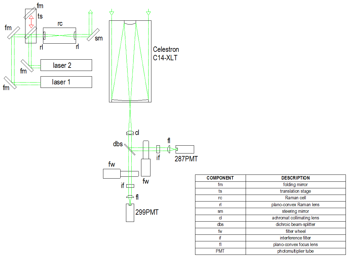
Figure 3A schematic showing the transmitter and receiver design for the DIAL ozone system. The abbreviations are explained in a separate box in the figure. Note the translation stage that can be moved to change which laser is used.
3.2 Aerosol lidar design
Since the aerosol lidar design described in Strawbridge (2013) was the backbone of this new system, only the changes will be discussed. The main differences are adding a laser for redundancy and adding an additional transmitted wavelength (355 nm), which in turn add the ability to acquire more particle information, and a water vapor channel arising from the Raman-shifted 355 nm output (407 nm) to provide nighttime water vapor profiles. The second identical laser, a Continuum Inlite III Nd:YAG operating at 20 Hz (see Fig. 1b), shares the same steering mirror (see Fig. 2) as the primary laser and can therefore be engaged remotely by a computer-controlled interface. The folding mirrors and steering mirror, manufactured by Blue Ridge Optics, are triple-coated (anti-reflection coating at 355, 532 and 1064 nm) and 50 by 6 mm flat, have a high damage threshold, and are mounted in a Thorlabs mount with encoded Thorlabs actuators to permit remote alignment if necessary. A schematic of the aerosol lidar in Fig. 2 shows the transmitter beam path and receiver design. The receiver was designed to image the aperture on the photomultiplier tube rather than the field stop. This is necessary to avoid signal modulations due to the inhomogeneous sensitivity of the cathode. The Continuum laser has an output energy of at least 65 mJ at 355 nm, 65 mJ at 532 nm and 100 mJ at 1064 nm. The seven-channel receiver (see Fig. 2) measures the backscatter at each of the emitted wavelengths as well as the depolarization at 355 nm, the nitrogen Raman channels at 387 and 607 nm, and the water vapor Raman channel at 407 nm. All of the channels except the 1064 nm channel use Licel photomultiplier tubes coupled into a Licel analog–photon-counting transient recorder to increase the dynamic range. The 1064 nm channel is focused onto a Perkin Elmer C30956E avalanche photodiode (APD). The APD incorporates a logarithmic amplifier (25 mV rms noise), made by Optech Inc., to increase dynamic range. The amplifier was calibrated prior to the experiment via a transfer function, to convert the signal to a linear scale, in addition to second-order corrections provided by Optech Inc. The signal is directed into a 14 bit Gage CompuScope computer card. The 1064 nm channel is generally used for qualitative information only because of issues such as APD sag and higher noise background. Both the Licel transient recorder and Gage computer card were externally triggered by the same Stanford Research Systems delay generator. The collected data are averaged to produce aerosol profiles from 100 m to 15 km above ground level (a.g.l.) every minute and water vapor profiles from 100 m to 10 km a.g.l. every 5 min.
3.3 Ozone DIAL design
The ozone DIAL system optical bench layout and detector design is shown in Fig. 3. A dual-laser design is also used for redundancy and can be engaged remotely by a user-controlled translation stage that moves the folding mirror in and out of the optical axis of the transmitter. The folding mirrors have an anti-reflection coating at 266 nm. The lasers are Continuum Inlite III Nd:YAG operating at 20 Hz with an output energy specification of 45 mJ at 266 nm. The laser pumps a 1 m long CO2-filled Raman cell (Nakazato et al., 2007) manufactured by Light Age. The two 45∘ mirrors together provide enough adjustment to align the laser beam to the optical axis of the Raman cell. The multi-wavelength output from the Raman cell is directed to the zenith by a steering mirror that is broadband coated from 266 to 320 nm. This 50 mm optic mounted in a Thorlabs mount with encoded Thorlabs actuators has a user-controlled interface to permit remote alignment if necessary. The differential pair chosen for the DIAL is the second and third Stokes lines from the Raman conversion, namely 287 and 299 nm. The two wavelengths are separated out via the detector block where the signals from the Licel photomultiplier tubes are directed into a Licel analog–photon-counting transient recorder. Again, the optical design imaged the aperture onto the photomultiplier tube for the same reason discussed in Sect. 3.2. A slight delay is imposed on the DIAL using a Stanford Research Systems delay generator to minimize cross-talk between the two lidar systems. The single-telescope design is capable of measuring ozone as low as 400 m a.g.l. to altitudes reaching 15 km during the night every 5 min. It operates 24 h a day, 7 days a week, except during precipitation events. The system is operated remotely, and the data are updated hourly to a website, providing near-real-time capability.
3.4 AMOLITE ozone DIAL algorithm and its validation
The raw data for AMOLITE are acquired every minute with a vertical resolution of 3.75 m. The data are then averaged (10 min for color-coded plots and sometimes longer for individual profiles) and processed using a boxcar filter to produce a simple smoothing of the raw data, followed by a second-order Savitzky–Golay convolution to compute the derivative with respect to altitude of the signal ratio and . Although the Savitsky–Golay approach may cause issues at the top of the stratospheric ozone profiles (Godin et al., 1999), it does not have as much of a negative impact for tropospheric ozone due to the vertical structure of ozone typically increasing at the top of the profile. This is primarily due to the signal-to-noise ratio being large enough at most altitudes. Alternate, more sophisticated filters are being considered (Leblanc et al., 2016a) and may be implemented in future data versions, but for now all TOLNet lidars are using the same approach. The boxcar smoothing used on AMOLITE data is a simple first-pass noise removal technique where a centered smoothing window is moved along the lidar signal profile and the average value across the window is calculated for each altitude. The averaged values then become the resulting smoothed profile. The size of the smoothing window starts at 10 bins and increases slightly with altitude (e.g., window is 150 at 12 km) to compensate for the lower signal-to-noise ratio encountered at increased range. The ozone data are also dead-time-corrected using a value of 4 ns. The background correction was determined by using the average background value calculated over a 10 km range starting at 35 km. For the Rayleigh extinction term we used the formulation described by Eq. (2.25) from Kovalev and Eichinger (2004). Also, the temperature-dependent ozone cross sections, at the AMOLITE wavelengths, were introduced using the Brion–Daumont–Malicet (BDM) values found in Weber et al. (2016). The BDM values were interpolated onto a 0.01 nm × 0.1 K grid.
The ozone data was not corrected for SO2 interference. There are only a few times during all the time periods presented in this paper where the ground level concentration of SO2 was above 5 ppbv. These events generally only lasted an hour or two and were thought to be associated with the industrial plumes. Unfortunately, we did not have vertical profile information for SO2, which can be highly variable in the lower troposphere, and so these data were screened out of the ozone plots. The clouds and regions near sharp aerosol gradients were also screened out of the ozone plots. Discussions are underway within TOLNet to reach a consensus on how to correct the ozone DIAL profiles when aerosols are present.
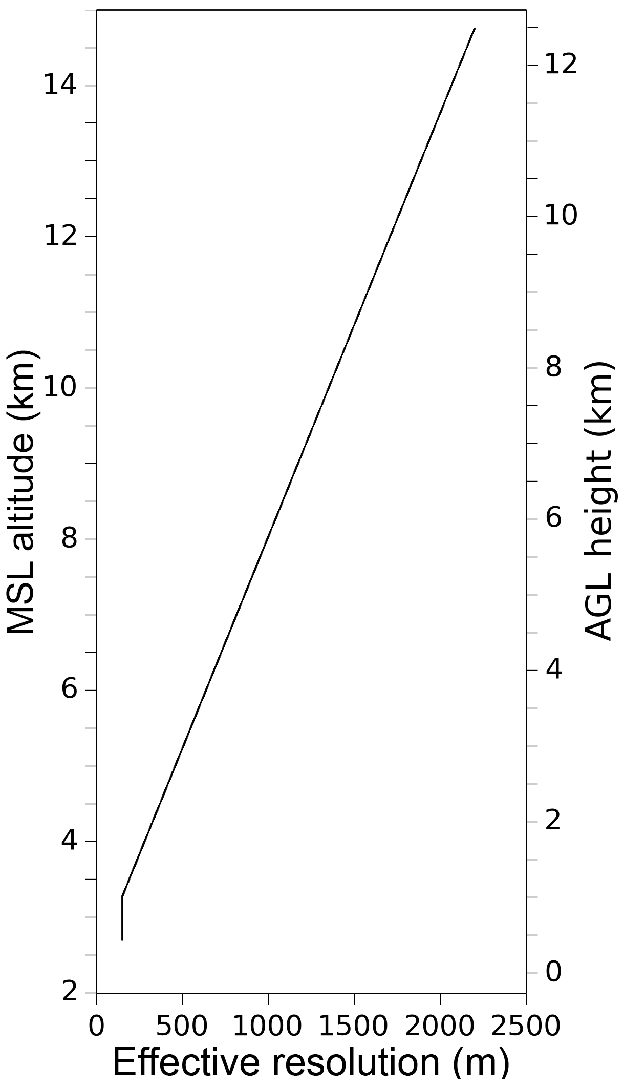
Figure 4A plot showing the effective resolution of the DIAL ozone profiles. The MSL (mean sea level) scale was used during the SCOOP campaign, and the AGL (above ground level) scale was used for the Oski-ôtin data.
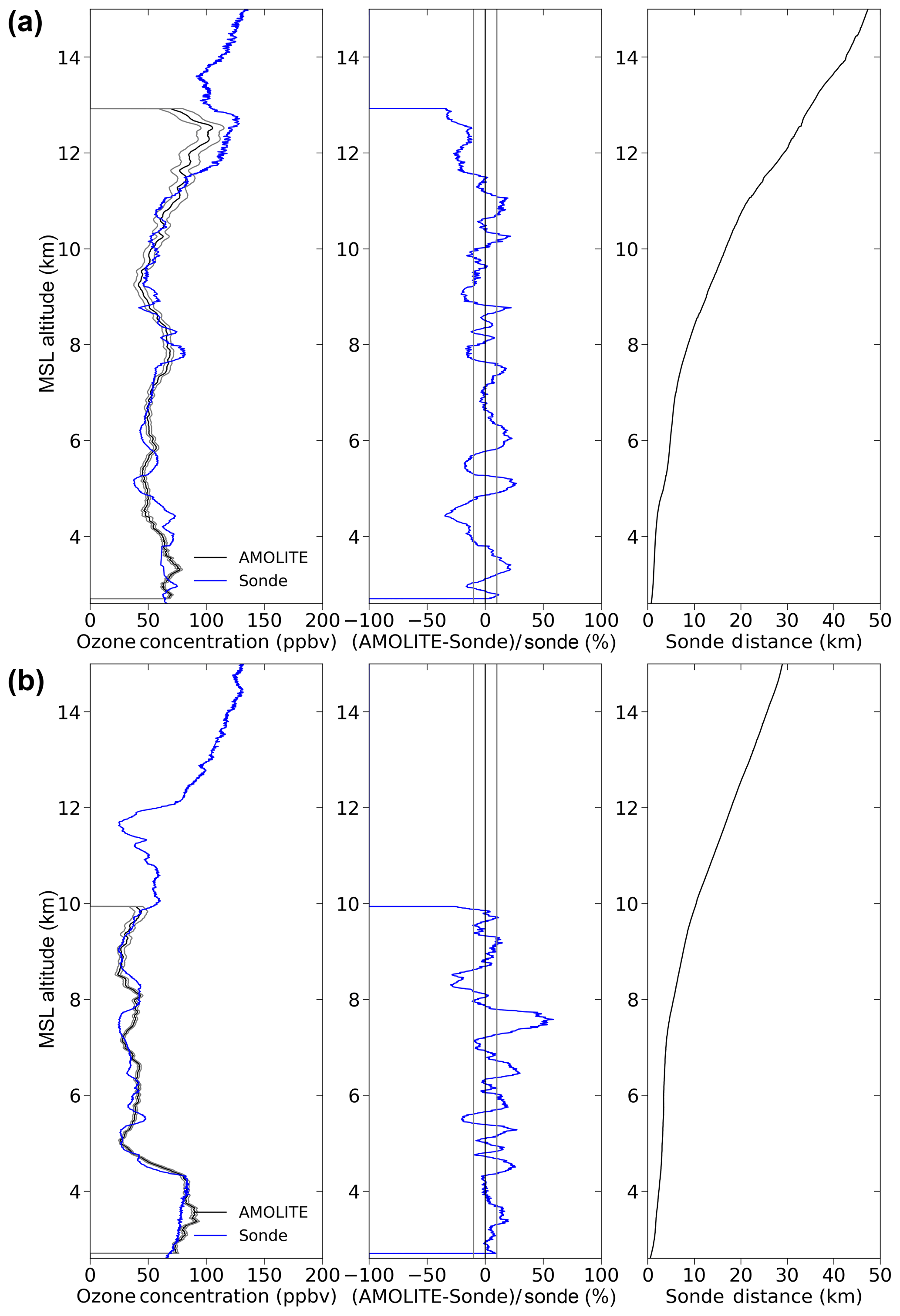
Figure 5Three-panel plots showing AMOLITE ozone profile against the sonde profile, the percentage difference between the two profiles and the horizontal sonde distance from the launch site for (a) 04:01 UTC on 10 August and (b) 21:03 UTC on 16 August. Local time is UTC − 7 h.
When undertaking a system validation, it is important to compare the final ozone profiles between DIAL systems and determine whether the differences are instrumental and/or algorithm dependent. As a result, AMOLITE's ozone algorithm was tested against a standardized algorithm developed for the SCOOP validation campaign. The first step required a data importer to be written that could read the simulated data into the AMOLITE algorithm. The simulated data included both the simulated lidar data and simulated sonde profiles. Next a boxcar smoothing that is applied to the AMOLITE data was turned off as there is no equivalent in the standardized algorithm. The algorithm testing began by turning off the dead-time correction (saturation), background correction, Savitzky–Golay smoothing, Rayleigh extinction correction and temperature-dependent ozone absorption cross sections (constant values were used for both wavelengths), leaving only the bare-bones ozone calculation. The concept was to use the simulated input in both the AMOLITE and standardized algorithms, comparing the results to the original simulated ozone profile with each algorithm. With all of the above terms turned off, the results matched perfectly after it was ensured that all unit conversions were done correctly and verified that both algorithms were using the same resolution functions. The next test involved using a different simulated ozone profile with saturation turned on. Comparing this to both algorithms with dead-time correction set to 4 ns gave confidence that the algorithms were both handling the saturation effects correctly. The next test involved turning off all the terms except the Rayleigh extinction correction and testing this new simulated ozone product against both the algorithms. Once it was established that both algorithms were calculating the Rayleigh profile from the simulated sonde input, the output matched with less than a 0.05 % bias, acceptable and not unexpected from math rounding errors. Proceeding to the next test, all terms were turned off except for the temperature-dependent ozone absorption cross sections. Here is was important to make sure the wavelengths of the system were taken to sufficient accuracy to minimize errors in the values picked form the standardized look-up table. In our case the wavelength values were set to the AMOLITE DIAL wavelengths of 287.20 and 299.14 nm. Once again with a successful outcome the final test was to turn on random (Poisson) noise and added sky background to the simulated ozone profile. For this final test all the terms were turned off except the background correction, and a second-order Savitzky–Golay convolution was applied, yielding a final result within 0.2 %. The end result of this testing gave us confidence that the AMOLITE ozone algorithm was performing flawlessly. Details of the results and comparisons to the other TOLNet lidar systems will be presented in the SCOOP validation paper (manuscript in preparation).
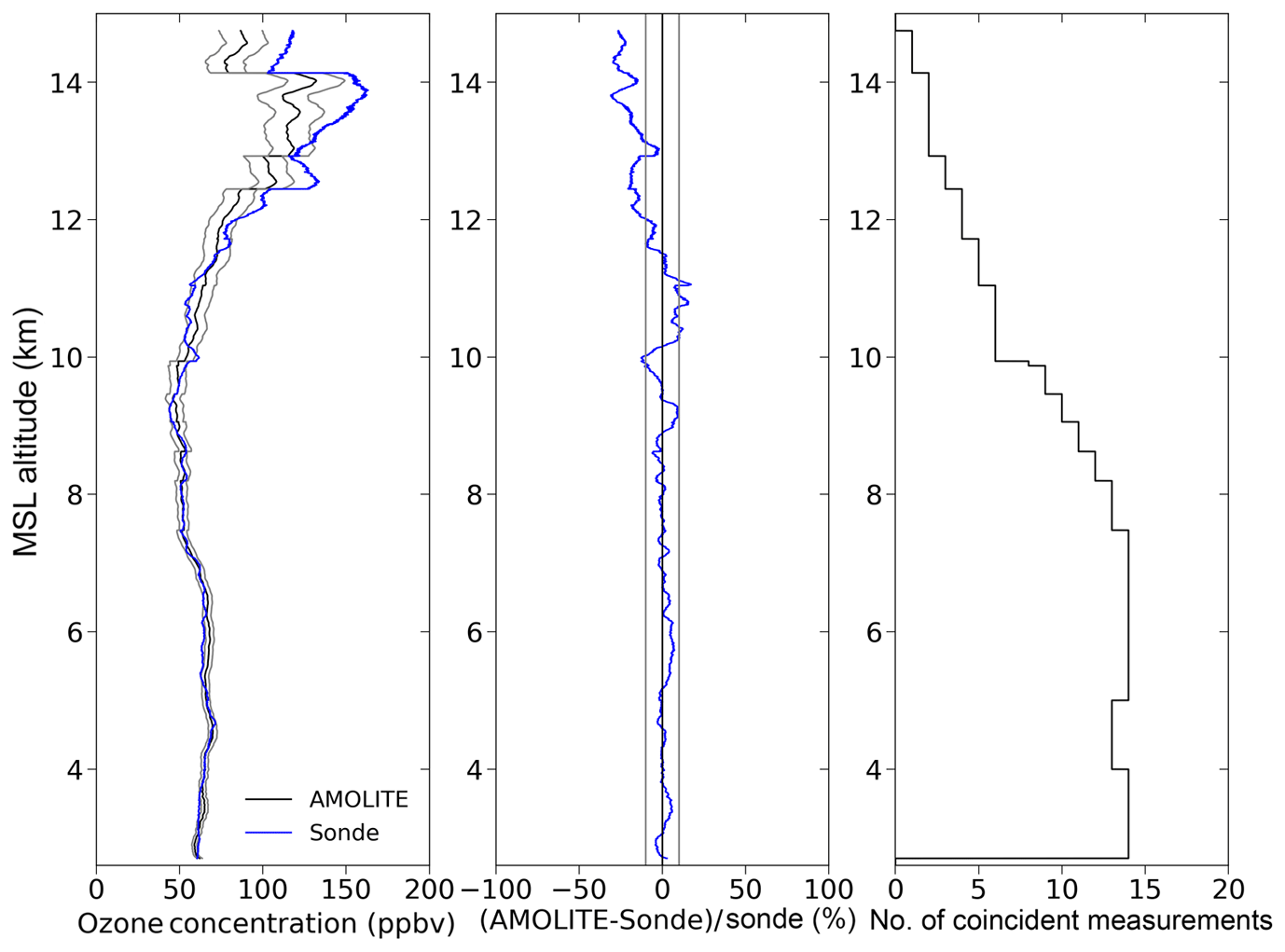
Figure 6Three-panel plot showing the average of all AMOLITE and coincident sonde profiles throughout the entire SCOOP campaign. The number of coincident measurements varies with altitude primarily due to the reduced altitude capability of the AMOLITE during daytime operation.
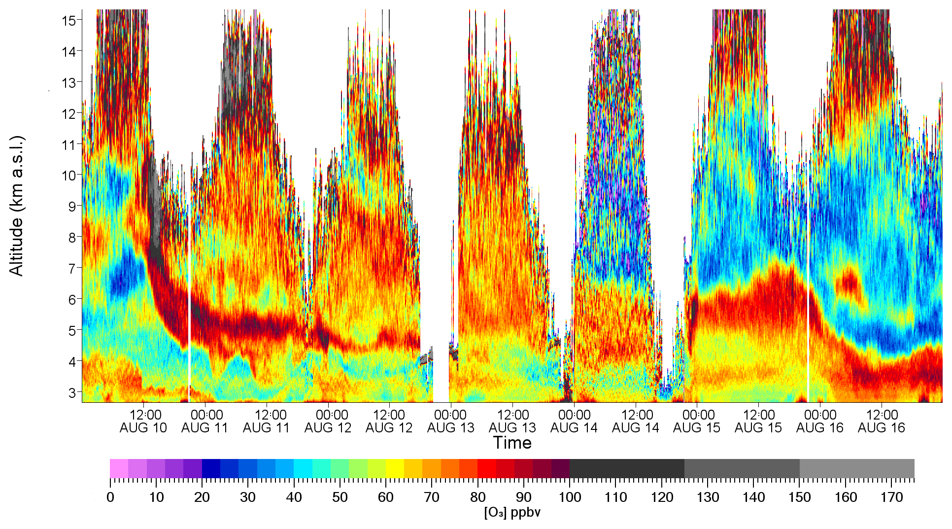
Figure 7False-color plot of ozone from AMOLITE during the entire SCOOP campaign. The white areas represent where no ozone data are available due to clouds or high daytime background light.
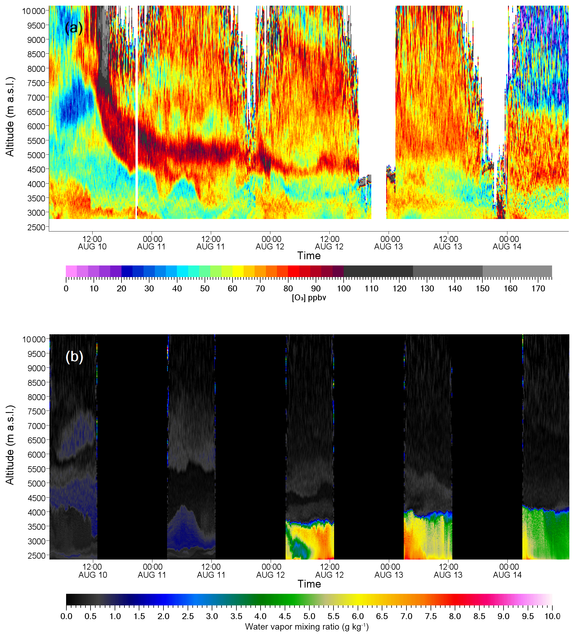
Figure 8False-color plots showing (a) ozone and (b) water vapor for the same time period of 10–14 August 2016.
3.5 AMOLITE instrument validation and calibration
The performance of the ozone lidar was evaluated through an intercomparison study with four other tropospheric ozone lidars, all of which are part of TOLNet. The campaign named SCOOP took place at the JPL Table Mountain Facility in Wrightwood, California. This provided an opportunity to compare AMOLITE ozone profiles between other lidar instruments and 14 ozone sondes launched during the study. The vertical resolution of the ozone lidar was chosen to be range dependent to provide sufficient detail in the lower troposphere as well as providing ozone profile information to altitudes reaching the tropopause, where the return signal is significantly weaker. Figure 4 shows the effective range-dependent resolution obtained using the algorithm developed by Leblanc et al. (2016a). The left y axis shows the effective resolution during SCOOP in meters above sea level that was applied to the AMOLITE ozone data in Fig. 5. Figure 5a represents a 30 min average of the lidar data starting from the time of the sonde launch at 04:01 UTC on 10 August 2016, and Fig. 5b is also a 30 min average at 21:03 UTC on 16 August 2016. These two profiles were shown to represent the typical results contrasting the range of the ozone DIAL during nighttime and daytime operation. Typically, the DIAL measurements at night will reach a range of over 10 km a.g.l. and dip to 7 km a.g.l. around midday, when the solar background is high. The agreement between AMOLITE and the ozone sonde on both days is very good, with the lidar generally staying within approximately 10 %–20 % of the ozone sonde values and no obvious bias throughout the profile. There are a few regions, notably around layer transitions, where the difference reaches 50 %. This is often due to the difference in vertical resolution of the two instruments. Note the sonde data are plotted at the highest vertical resolution available. It is also important to note that the geophysical separation of the sonde at altitudes of 12 km above sea level is 20–30 km for these cases, which can easily account for the larger differences between the sonde and lidar as the altitude increases. On some days during the study the lidar–sonde agreement varied significantly, particularly at the higher altitudes, due to the large geophysical separation of the two measurements. This is shown in Fig. 6, which represents the average of all 14 lidar–sonde comparisons. The middle panel clearly shows that up to 8 km the lidar agrees to within 5 % of the sonde, with larger differences aloft where there are fewer number of coincidences and the geophysical separation with the sonde increases.
The entire SCOOP campaign is captured in the false-color ozone DIAL plot shown in Fig. 7. AMOLITE was the only fully autonomous lidar operating during SCOOP. The advantages of a fully autonomous lidar system are easily recognized in its ability to capture a continuous dataset throughout the complete diurnal cycle while capturing the dynamics and mixing of long-term events. The ozone DIAL reaches the lower stratosphere, enabling observations of STT events. The signal-to-noise ratio was affected during 11–14 August, when there was an air conditioner failure. The outside temperature reached over 30 ∘C, and the single remaining air conditioner was unable to keep up with the cooling demand of two lidars operating simultaneously. A decision was made to turn off the aerosol/water vapor lidar for the remainder of the study to focus on the ozone intercomparison.
The two color-coded plots in Fig. 8 show the advantage of coincident measurements of ozone and water vapor: in this case, a stratospheric intrusion which starts just after 12:00 UTC on 10 August, descends to approximately 4 km above sea level and persists for over 3 days. The water vapor plot (see Fig. 8b), even though it represents nighttime measurements only, clearly shows the very dry air coincident with the high ozone concentrations of the stratospheric intrusion. The water vapor measurements below 4 km on 10 August show very dry air (and high ozone values), which may also represent a prior stratospheric intrusion, followed by a more defined boundary layer with an increase in water vapor, more typical of boundary layer air. The water vapor channel was calibrated as described by Al Basheer and Strawbridge (2015) using the SCOOP radiosonde data.

Figure 9False-color plots the first 10 km of the atmosphere for (a) ozone, (b) water vapor and (c) aerosol backscatter ratio for the period of 6–13 November 2016 at the Oski-ôtin ground site.
3.6 AMOLITE ozone uncertainty
An uncertainty in the ozone concentration from AMOLITE can be calculated mathematically for several components. For consistency with other DIAL systems within TOLNet, the uncertainty calculation was based on the paper by Leblanc et al. (2016b). For a detailed description of the mathematical formulations please refer to that paper. In brief, the total uncertainty determined for AMOLITE (e.g., see Figs. 5 and 6) was based on six different components: uncertainty due to detector noise, uncertainty due to saturation, uncertainty due to the Rayleigh cross section, uncertainty due to the background calculation, uncertainty due to the ozone cross section and uncertainty due to the air number density. To calculate these uncertainties, one must also make estimates of dead-time error (estimate: 10 %), the Rayleigh error (estimate: 1 %), the sonde pressure uncertainty (estimate: 20 Pa) and the temperature uncertainty (estimate: 0.3 K). The AMOLITE uncertainty calculations, for each individual uncertainty, were successfully compared to the standardized algorithm uncertainty for a test profile. The altitude at which the AMOLITE ozone profiles get truncated is based on a total uncertainty threshold value, chosen to be 15 % based on AMOLITE–sonde comparisons. There is no threshold value set for the ozone false-color plots. This can sometimes provide additional context for the existence of layers, particularly at higher altitudes.
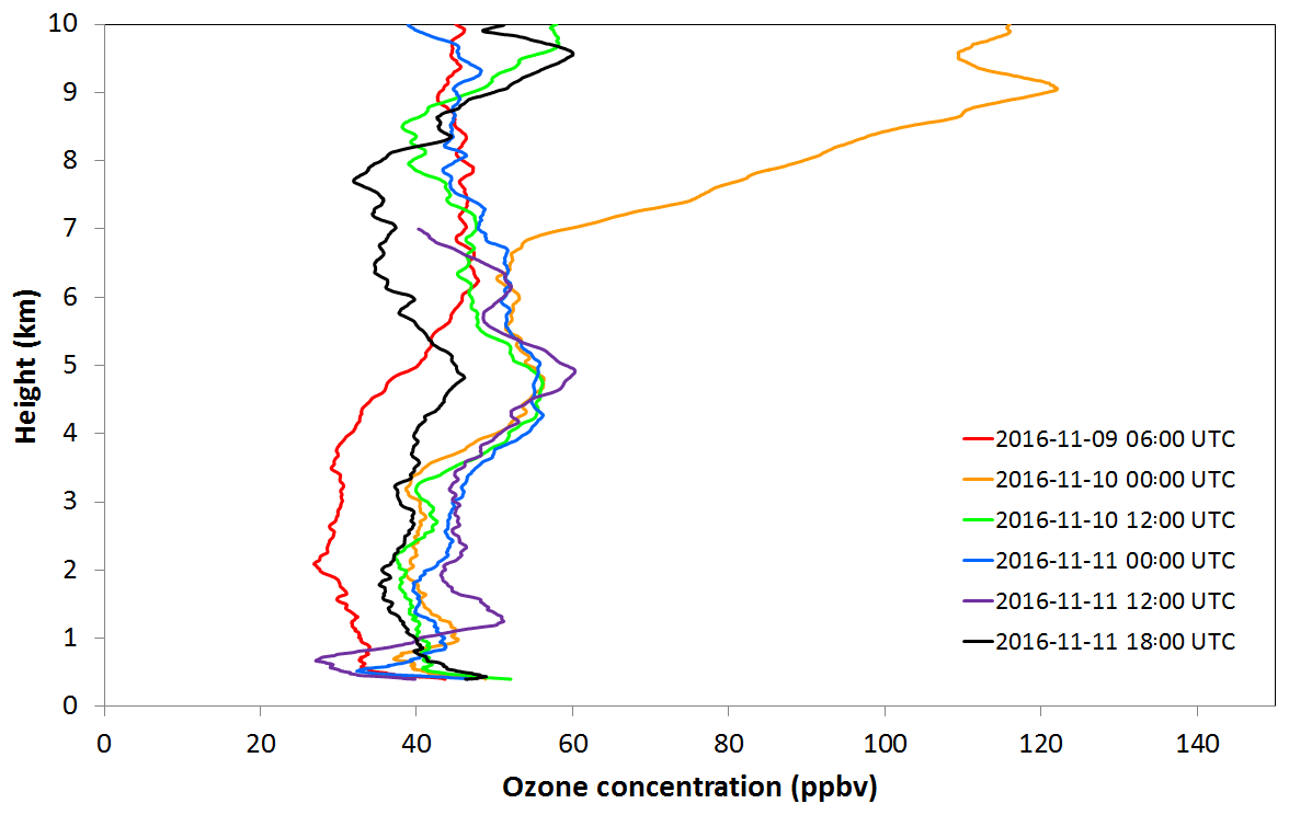
Figure 10A plot showing ozone profiles between 9 and 11 November as the ozone-rich stratospheric air descends down into the troposphere.
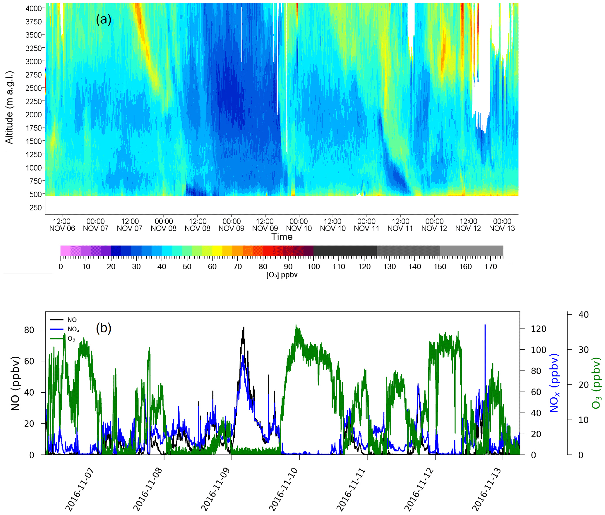
Figure 11(a) False-color plot showing of DIAL ozone from AMOLITE between 6 and 13 November, and (b) surface measurements of ozone and NOx during the same time period.
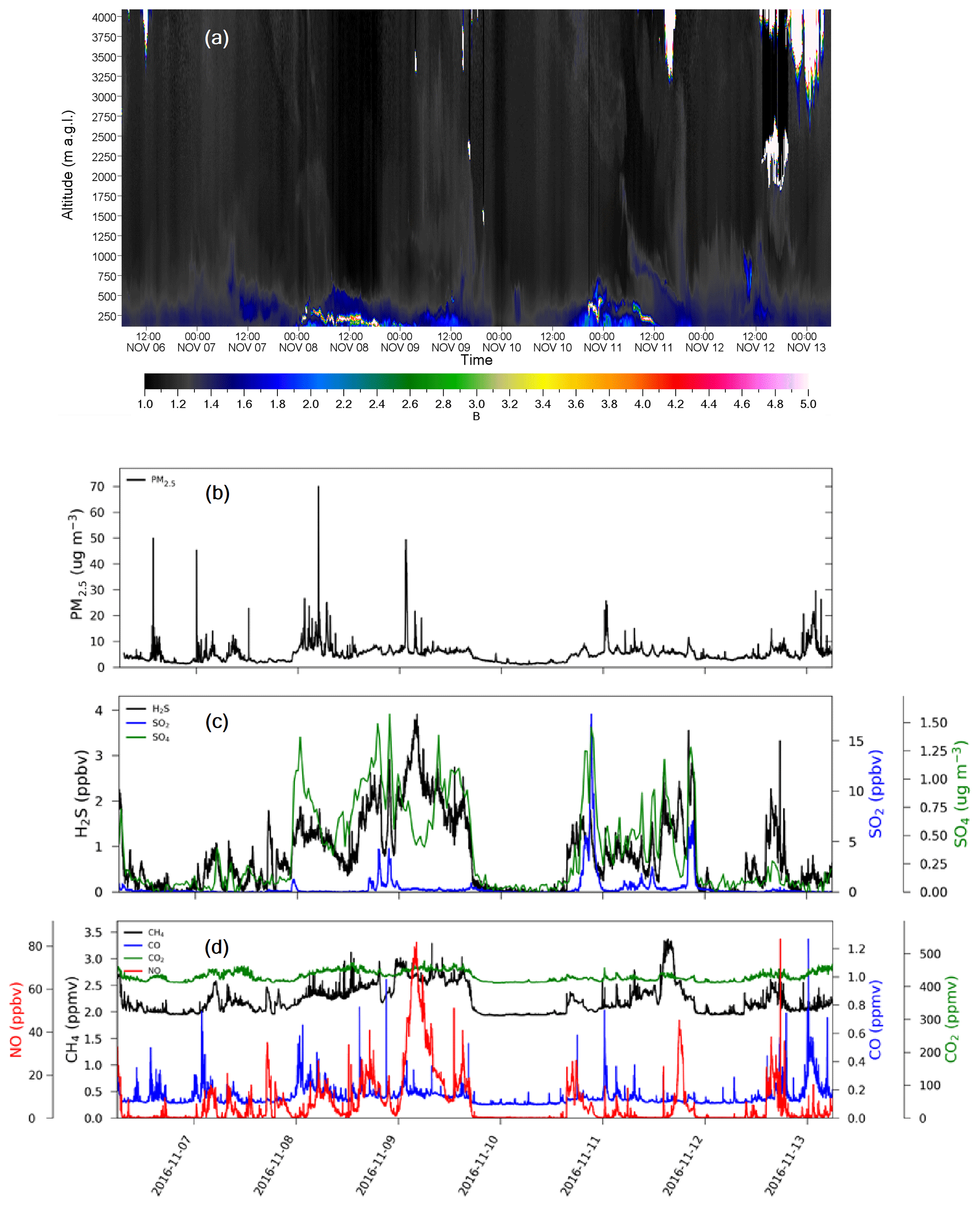
Figure 12(a) False-color plot of aerosol backscatter ratio for the same altitude and time period as Fig. 11a. CAM1 surface measurements during the same time period for (b) PM2.5; (c) sulfates; and (d) CH4, CO, CO2 and NO.
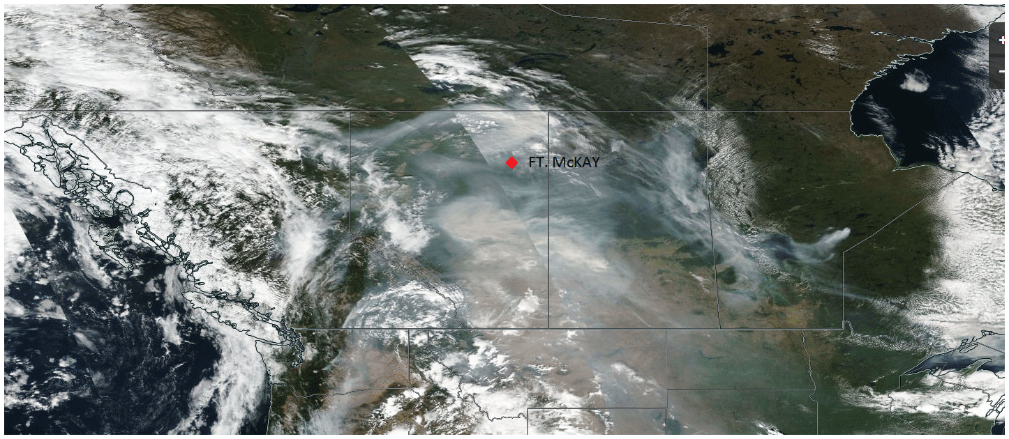
Figure 13Terra MODIS true-color composite image on 31 August 2017. Note the location of the ground site.
After the SCOOP campaign, AMOLITE was transported back to ECCC's Centre For Atmospheric Research Experiments, where the air-conditioning unit was repaired and routine maintenance was done on the instrument to prepare it for deployment to the oil sands region in northern Alberta. AMOLITE started collecting the full suite of data products on 3 November 2016. The instrument has run fully autonomously, collecting a year's worth of consecutive data except for a couple of weeks in July when the instrument was down for a service visit due to a laser failure and two shorter periods of time for routine maintenance requirements. During the first year of operation, the autonomous ozone, aerosol and water vapor lidar measurements provided a near-continuous dataset, observing the impact of many atmospheric processes and transport over a range of scales and altitudes. The following sections give examples of three selected periods throughout the year, showing the impact of long-range transport events, atmospheric dynamics and local industrial sources as well as seasonal variability.
4.1 6–13 November 2016
Stratospheric intrusions were frequently observed throughout the year, with sometimes three or four occurrences per week. In recent years, there has been more understanding about the mechanism that enables these STT events (Langford et al., 2018). However, there is still very little data on the frequency and magnitude of these events and their impact on the tropospheric ozone budget. For example, Fig. 9 shows three false-color plots of ozone, water vapor and aerosol backscatter ratio for the bottom 10 km of the atmospheric from 6 to 13 November 2016. During this week-long period two stratospheric intrusions were observed (and evidence that a third started on 13 November). The white areas on the ozone plot, represent cloudy regions where the DIAL system is unable to retrieve ozone values. These white areas correlate very well with the cloud regions displayed in the aerosol backscatter ratio plot. The water vapor plot shows dry air (less than 0.2 g kg−1) coincident with the higher ozone concentrations of the stratospheric air reaching down into the moist regions more typical of the lower atmosphere. During most of the stratospheric intrusions over the Oski-ôtin site, it was noted that, although the free-tropospheric ozone levels were increased significantly, the ozone intrusion does not always penetrate the boundary layer and increase surface values.
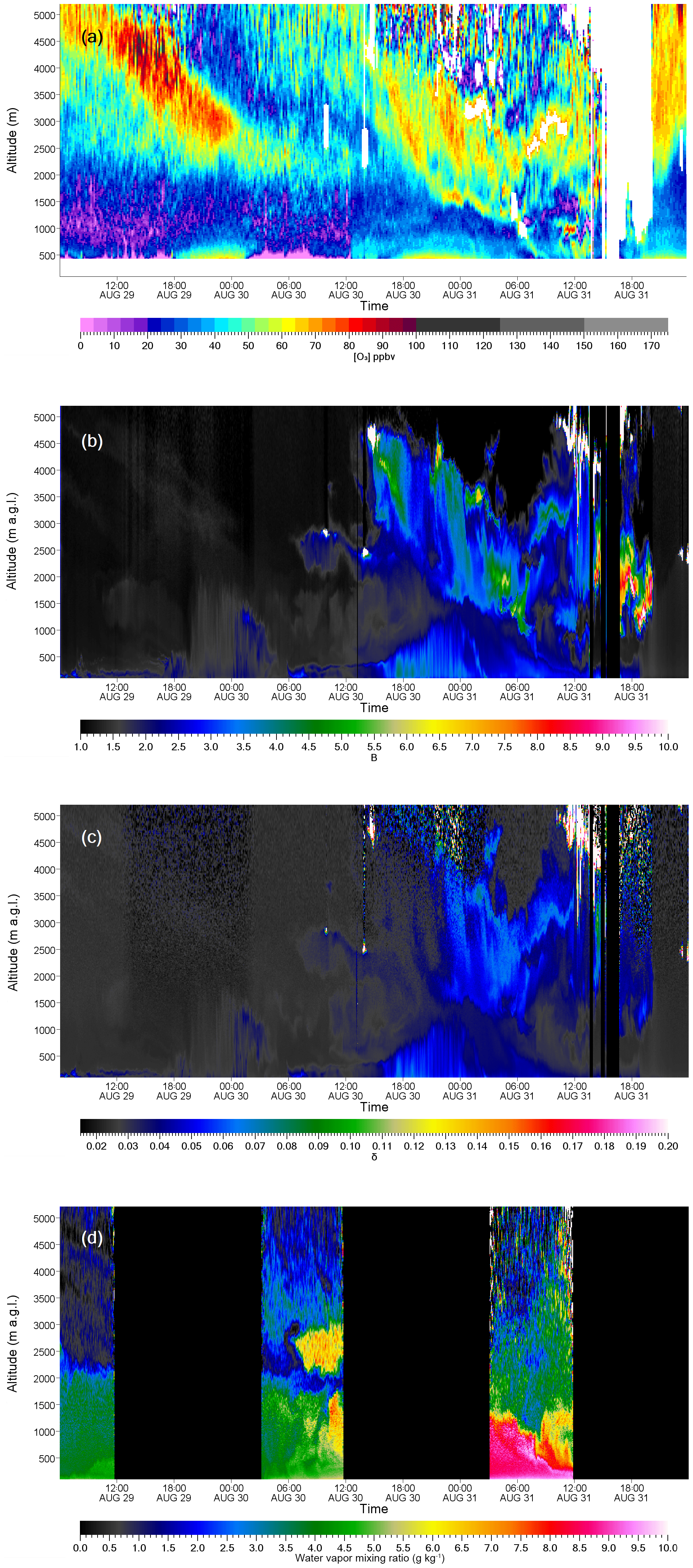
Figure 14False-color lidar plots for 29–31 August for (a) ozone, (b) backscatter ratio, (c) depolarization ratio and (d) water vapor (nighttime only).

Figure 15(a) DIAL ozone traces at different altitudes compared to surface ozone for the same period as Fig. 14. CAM1 surface measurements for same time period of (b) ozone and NOx; (c) sulfur compounds; (d) PM2.5; and (e) CH4, CO, CO2 and NO.
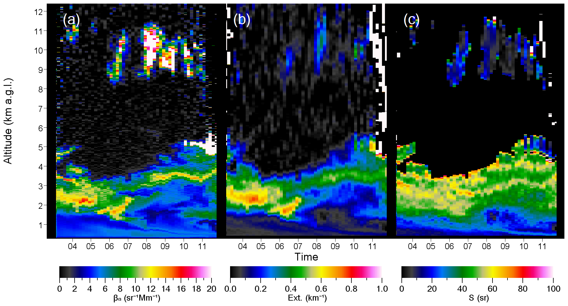
Figure 16Three-panel plot showing the backscatter coefficient, extinction coefficient and S ratio for 31 August.
A series of ozone vertical profiles during the stratospheric intrusion between 9 and 11 November is plotted in Fig. 10. This plot shows the ozone concentration before the intrusion (red line) where the typical background value of approximately 30 ppbv is present in the lowest 4 km. As time progresses, one can clearly see the high ozone concentration, reaching 120 ppbv on 10 November at 00:00 UTC, from the stratospheric transport descending down to lower and lower altitudes. The impact increased the tropospheric budget by almost a factor of 2. Figure 11 shows only the lowest 4 km of the ozone plot compared to the ground level observations of ozone and NOx. There is reasonably good agreement between the ground level measurements and the DIAL measurements around 600 m (the lowest few lidar bins can be unreliable as they are strongly dependent on the alignment and temperature fluctuations inside the trailer). It is also important to consider the height of the boundary layer (see Fig. 12a), which during the wintertime can be significantly lower. The ozone–NOx relationship in Fig. 11b is not the typical diurnal relationship that can be observed, in part due to the stratospheric intrusion event, but also due to industrial plume sources impacting the site. For several hours on 7, 8 and 9 November the ozone values approach 0. There is an increase in ozone not only during the daytime hours (solar day is approximately 14:00 to 00:00 UTC during this period) but also during the nighttime on 10, 11 and 12 November, when the stratospheric intrusion occurred. Figure 12 shows the aerosol lidar plot for the lowest 4 km along with various chemical and particulate tracers from CAM1. The aerosol lidar plot gets down to approximately 100 m above ground level, which during the winter months is necessary to observe the boundary layer and plume dynamics. There is a good correspondence between the increase in aerosol shown by the lidar and the PM2.5 trace over the entire period. The increase in particle concentration is linked to the presence of the plume impacting the site. For example, on 7–9 November and the night of 10 November the aerosol lidar observations show an increase in concentration in the lowest 750 m (see Fig. 12a) typical of industrial plume sources. As the plume impacts the ground directly, there is a substantial bump in the PM2.5 concentration. Figure 12c and d also indicate that the air is from an industrial source where the CO2, CO, CH4 and sulfur compound concentrations are high. This is the first example where the vertical context given by the lidar aids in the understanding of the ground-based measurements.
4.2 29–31 August 2017
Another occurrence that can change the ozone budget is forest fires (Jaffe and Wigder, 2012). During the period of 29–31 August, smoke from a forest fire was advected into the region as shown in the MODIS (Moderate Resolution Imaging Spectroradiometer) true-color image acquired form the Terra satellite on 31 August 2017 (see Fig. 13). The ozone plot shown in Fig. 14a presents a significant amount of ozone in the free troposphere. The enhanced ozone signature on 29 August is from a stratospheric intrusion, whereas the enhanced ozone on 30 and 31 August is a result of forest fire smoke. The extent of the forest fire smoke is shown by the large aerosol burden in Fig. 14b coincident with the ozone as well as the depolarization ratio plot in Fig. 14c, showing a value of about 5 %, consistent with other smoke plume measurements (Aggarwal et al., 2018).
The diurnal cycle of ozone over 3 days is shown in Fig. 15b with increased ozone due to the smoke impacting the surface around 00:00 UTC 31 August, from what we hypothesize to be enhancement from the forest fire. In Fig. 15a a series of ozone traces at different altitudes from the DIAL measurements are plotted against the ground ozone values. In this plot the ozone aloft tracks the ground level ozone quite well until the ozone-enhanced air from the forest fire smoke begins to descend over the site. The noisy ozone values around the 1000 m level are a result of an error in ozone when the aerosol concentrations were very high (see Fig. 14a and b around 15:00 to 17:00 UTC on 31 August). There is also evidence that the smoke impacted the surface from 00:00 to 18:00 UTC on 31 August as shown in Fig. 15c–e, where an increase in H2S, PM2.5 and CO also occurs. An alternative way to plot aerosol lidar data is to plot extinction coefficients instead of backscatter coefficients. Since we are measuring the nitrogen Raman channel during the nighttime, we can calculate the backscatter coefficient; extinction coefficient; and extinction-to-backscatter ratio, also known as the S ratio. The S ratio is a useful quantity for determining the aerosol type (see Strawbridge, 2013). The three-panel plot in Fig. 16 shows the 355 nm backscatter coefficient, extinction coefficient and S ratio for 03:00 to 12:00 UTC (nighttime) on 31 August 2017 using 10 min average data. The near-field overlap is corrected, and the data are plotted in kilometers above mean sea level (m.s.l.), primarily because the atmospheric density obtained from sonde data is also relative to m.s.l. The white noisy regions aloft on the extreme left and right are artifacts due to the increase in sky background. The backscatter coefficient plot reveals the dynamic nature of the smoke plume between 1 and 5 km and a cirrus cloud layer between 8.5 and 11 km. The extinction coefficient plot is useful because one can directly relate it to aerosol optical depth by integrating along the altitude range. The S ratio plotted as a 10 min average shows extraordinary detail within the smoke plume, with values ranging approximately from 40 to 65 sr. These values are consistent with the value of 45 to 65 sr reported by Barbosa et al. (2014) and are consistent with several other observations provided in Table 3 of Ortiz-Amezcua et al. (2017). Figure 16 also shows the boundary layer aerosols with an S ratio of 20 to 35 sr, indicative of larger particles in the moist boundary layer air (see water vapor plot in Fig. 14d), and 10 to 15 sr in the cirrus cloud. Figure 17 shows a 1 h average taken between 08:00 and 09:00 UTC. For highly variable conditions such as a forest fire plume, the 1 h average may result in underestimating the maximum S value. It is also very difficult to measure the S value in the free troposphere when there is very little aerosol present, such as in this case. Those values will be very noisy and have been discriminated out of the dataset shown here.
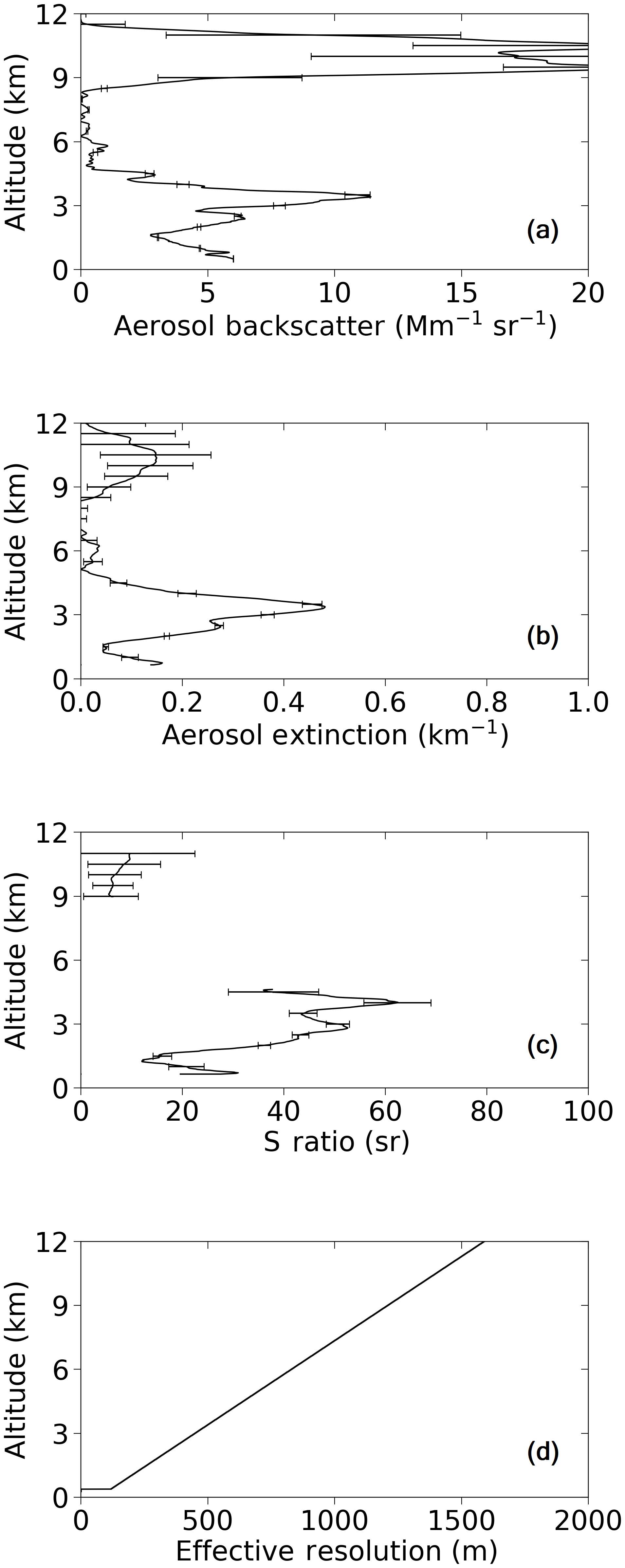
Figure 17One-hour average between 08:00 and 09:00 UTC on 31 August for (a) backscatter coefficient, (b) extinction coefficient, (c) S ratio and (d) effective resolution.
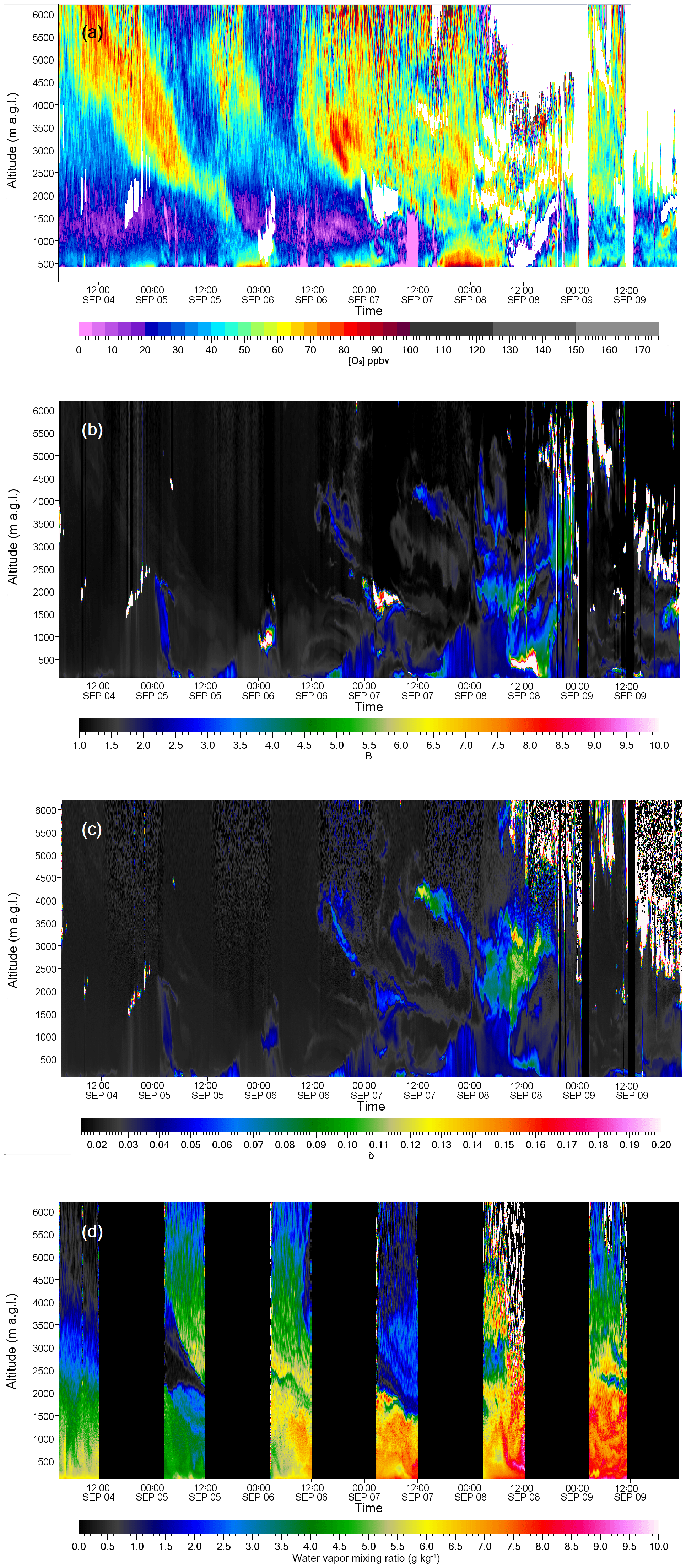
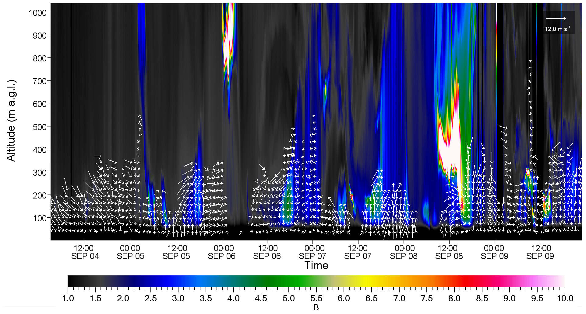
Figure 18False-color lidar plots for 4–9 September for (a) ozone, (b) backscatter ratio, (c) depolarization ratio and (d) water vapor (nighttime only).
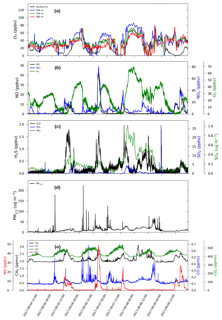
Figure 19(a) DIAL ozone traces at different altitudes compared to surface ozone for the same period as Fig. 18. CAM1 surface measurements for same time period of (b) ozone and NOx; (c) sulfur compounds; (d) PM2.5; and (e) CH4, CO, CO2 and NO.
4.3 4–9 September 2017
The ozone plot for 4–9 September 2017 (see Fig. 18a) shows several processes occurring throughout the entire altitude range. There is a stratospheric intrusion on 4 September that extends in 5 September (see dry air in Fig. 18d). The increased ozone in the free troposphere from 6 to 9 September is due to the forest fire activity being advected back into the region. The forest fire smoke is clearly visible in the aerosol backscatter plot (see Fig. 18b) and the depolarization ratio plot (see Fig. 18c). There is also a fairly dominant feature between 800 and 2200 m where the ozone values reach very close to 0. There are also time periods where these near-0 ozone features appear to reach closer to ground level (12:00 UTC on each day during the 4–7 September period). This is also shown in Fig. 19a, where the ozone values from the DIAL at 500, 700 and 900 m are plotted against the ground level ozone. The very low surface ozone around 12:00 UTC on 7 September remains low well up into the lower troposphere. The ozone data around 12:00 UTC on 8 September are an artifact due to the very high aerosol loading and have been removed. The surface ozone levels (see Fig. 19b) on 4 September ranged from a low of 10 ppbv around 12:00 UTC to 20 ppbv. Figure 20 shows the winds were primarily coming from the north, where there are fewer industrial sources to impact the ground site. However, on 5 September the winds were coming from the south, where the industrial sources impact the site as shown by the increase in NOx (see Fig. 19b), sulfates (see Fig. 19c), PM2.5 (see Fig. 19d) and CO2 (see Fig. 19e).
The ground level ozone increased to 70 ppbv around 18:00 UTC on 7 September and dropped to 50 ppbv around 03:00 UTC on 8 September, which was mostly due to the southerly wind (see Fig. 20) bringing the industrial plumes to the ground site. The DIAL ozone shows ozone levels reaching 80 ppbv within 500 m of the surface. There is also an increase in SO4 and CH4 during this time period. The diurnal ozone cycle is very well established throughout this entire study period, except when the elevated ozone from the forest fire smoke is mixed down to the surface starting around 06:00 UTC on 8 September (note the increase in NO2 but not NO). The increase in ground level ozone throughout the nighttime reaches values of up to 35 ppbv. There is also a steep increase in PM2.5 levels (from 25 to 50 µg m−3) and CO around 15:00 UTC on 8 September coincident with the lidar backscatter ratio plot shown in Fig. 18b indicative of an increased concentration of the biomass burning plume impacting the ground site. The wind has also shifted from a southerly flow to eventually a northerly flow. The resultant ozone at the ground is a mixture of local chemistry and ozone-rich air transported into the region.
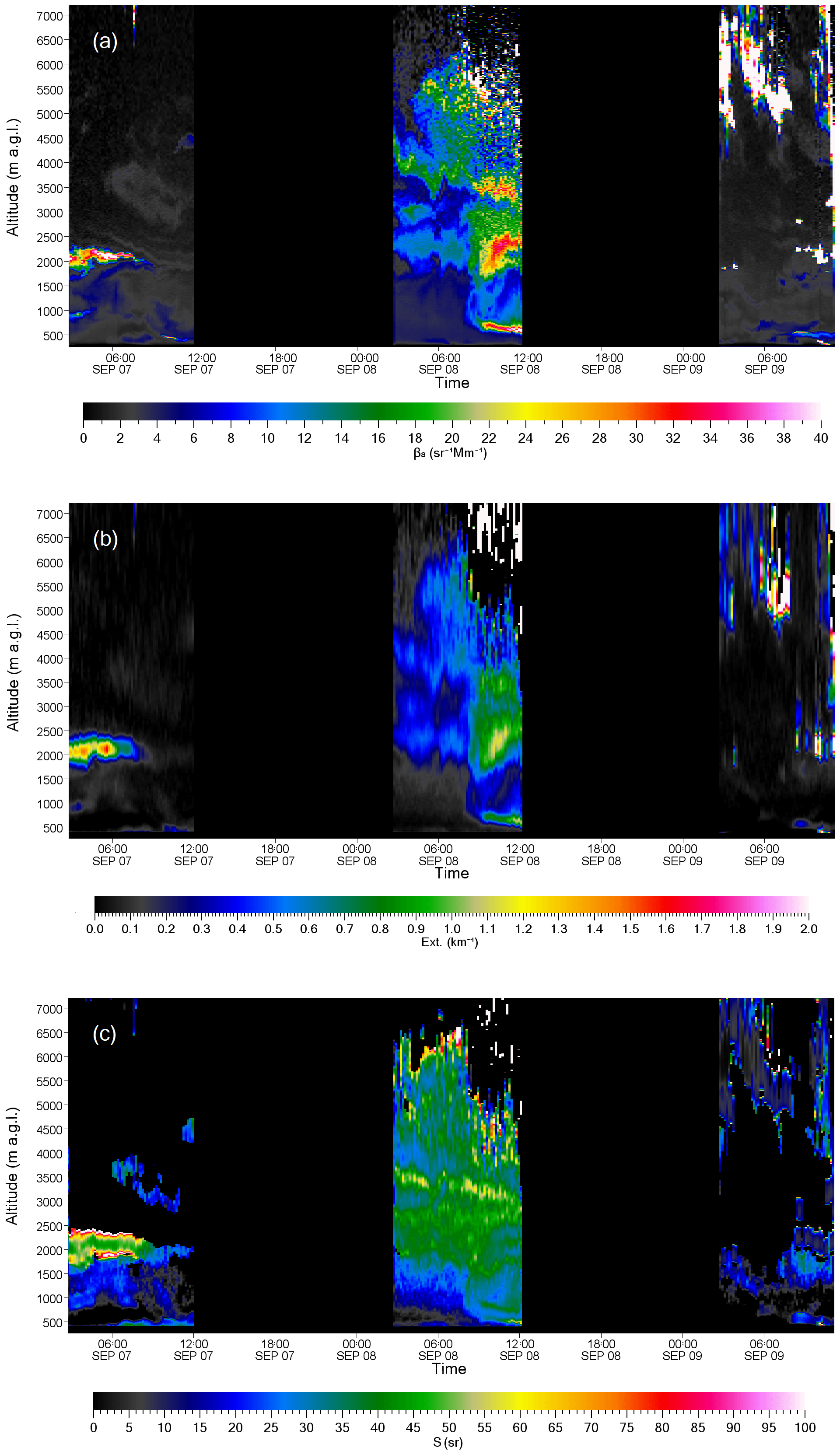
Figure 21False-color plots of 4–9 September for (a) backscatter coefficient, (b) extinction coefficient and (c) S ratio.
A plot of the backscatter coefficient, extinction coefficient and S ratio from 7 to 9 September (see Fig. 21) shows the contrast between the smoke plume on 8 September and the boundary layer aerosols and industrial plume (around 2 km on 7 September). The smoke plume S ratios are slightly smaller (35 to 55 sr) compared to 31 August, likely indicative of more aged smoke (see the 1 h average plot between 10:00 and 11:00 UTC shown in Fig. 22c). The lidar ratio, S, can also be calculated for 532 nm. However, there is a significantly lower signal-to-noise ratio, so the 10 min average false-color plots were not produced. A comparison was made for a 1 h average when the smoke plumes were present on 31 August and 8 September (see Fig. 23a and b). The S ratio for 532 nm on 31 August ranges from 40 to >100 sr, while on 8 September it ranges from 40 to 70 sr. These values are consistent with the higher 532 nm S ratio values reported in Table 3 of Ortiz-Amezcu et al. (2017). The Ångström exponent (see Fig. 23c and d) is inversely related to the average size of the particles. On 31 August the extinction Ångström exponent was 1.56±0.2 between 2 and 4.2 km, in contrast to 1.35±0.2 between 2 and 4 km on 8 September. These values are consistent with what others have reported for biomass burning (see Table 3 by Ortiz-Amezcu et al., 2017). During this 6-day period it would be very difficult to understand the ground measurements without the vertical context of the lidars.
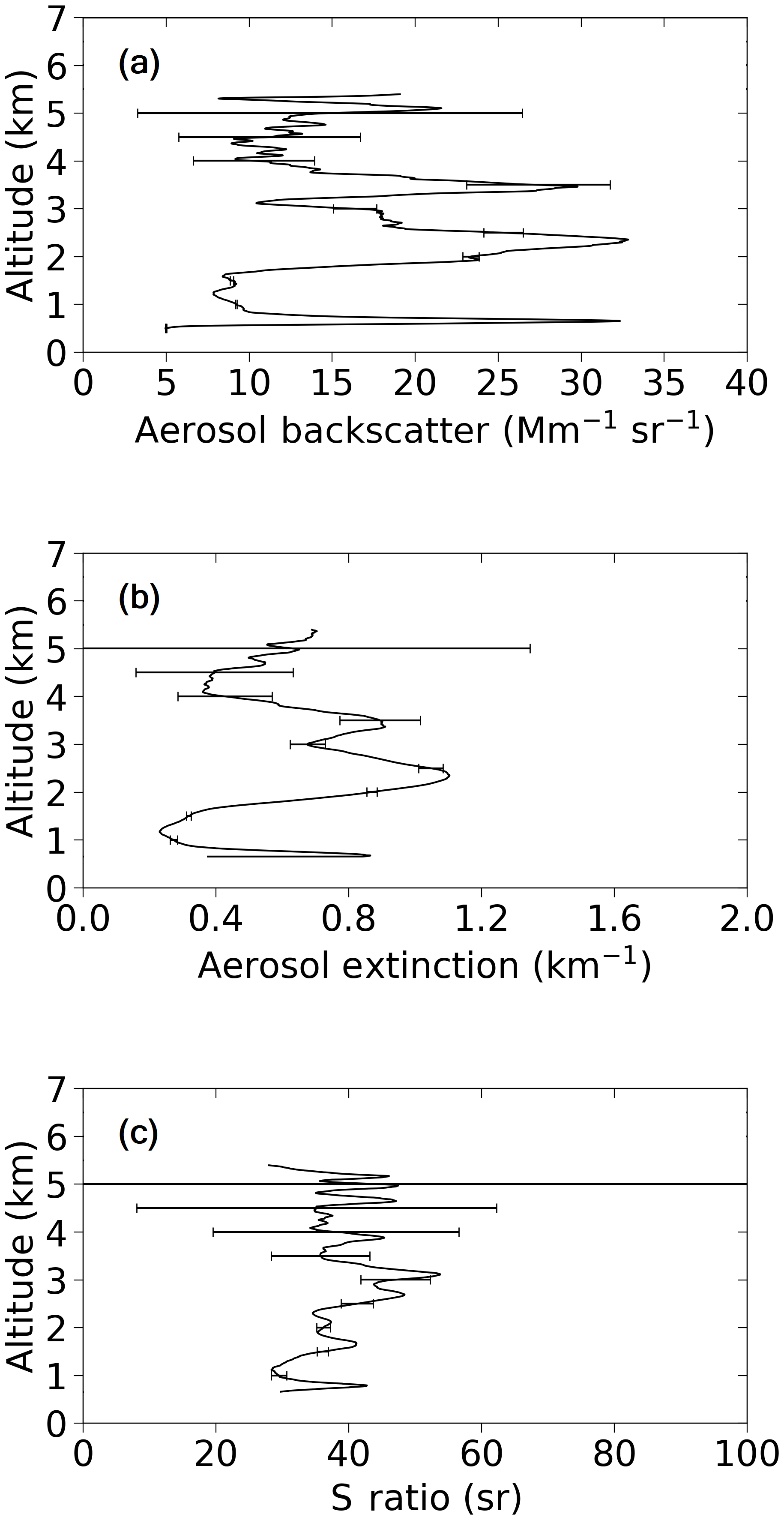
Figure 22One-hour average between 10:00 and 11:00 UTC on 8 September for (a) backscatter coefficient, (b) extinction coefficient and (c) S ratio. The effective resolution is the same as Fig. 17.

Figure 23(a) S ratio plot of 355 and 532 nm for 31 August, (b) S ratio plot of 355 and 532 nm for 8 September, (c) extinction Ångström exponent for 31 August and (d) extinction Ångström exponent for 8 September. Same 1 h averages as Figs. 17 and 22.
Environment Canada has successfully designed, built and deployed a fully autonomous ozone, aerosol and water vapor lidar system called AMOLITE. The instrument participated in a validation campaign with other tropospheric ozone lidars where the continuous operation of AMOLITE provided a unique dataset showing the complete evolution of atmospheric events. The instrument underwent an extensive validation in both the hardware and software algorithm processing to provide confidence in the AMOLITE ozone profiles generated. A comparison with ozone sondes revealed no bias in the AMOLITE ozone profile and a typical difference of less than 10 % throughout the altitude range. It was also shown that stratospheric intrusions can have frequent and significant impact on free-tropospheric and sometimes even surface measurements. In some cases the ozone concentration at the surface can be increased by a factor of 2. It was also shown that higher ozone levels in forest fire plumes can also impact local air quality. The lidar ratio was also calculated for the forest fire plume and found to range from 35 to 65 sr at 355 nm and 40 to 100 sr at 532 nm. It was also noted that over an 8-day period the S ratio decreased. The average Ångström exponent went from 1.56 on 31 August to 1.35 on 8 September. The three-lidar system provides critical information and vertical context to help interpret ground-based surface measurements. The primary motivation in building AMOLITE was to collect continuous lidar profiles, except during precipitation, to improve our understanding of the impact and extent of long-range transport and other pollution events on air quality at local, regional and national scales. Developing an autonomous lidar facility significantly reduces the operational field costs of maintaining on-site personnel. The development of the instrument was possible due to recent technological advancements in laser technology and Internet-controlled electronics. A sophisticated control program was developed to provide safe operations; extensive system controls; and the storage, transmission and display of the data in near-real time. One of the challenges with an autonomous multi-lidar system is the large volume of data produced. While the quick-look products that are currently produced are very useful to survey data quality and periods of interest, it will be necessary to develop algorithms to meet the data archival needs and produce various product data levels. Some of these will include automated cloud screening, aerosol corrections and possibly other derived products such as boundary layer height. The implementation of these algorithms in the future will provide further value for the current location as well as future observation sites.
Current plans are underway to add a second telescope to the ozone DIAL to allow measurements closer to the surface. A couple of different designs are being investigated that will fill in the gap between 100 and 500 m. This is quite important, particularly during the winter months and nighttime operation, when the boundary layer can often be less than 500 m in height.
The data are not publicly accessible.
The authors declare that they have no conflict of interest.
This article is part of the special issue “Atmospheric emissions from oil sands development and their transport, transformation and deposition (ACP/AMT inter-journal SI)”. It is not associated with a conference.
The project was supported by the Environment and Climate Change Canada's
Climate Change and Air Quality Program (CCAP) and the Joint Oil Sands
Monitoring program (JOSM).
Edited by: Mark Weber
Reviewed by: two anonymous referees
Aggarwal, M., Whiteway, J., Seabrook, J., Gray, L., Strawbridge, K., Liu, P., O'Brien, J., Li, S.-M., and McLaren, R.: Airborne lidar measurements of aerosol and ozone above the Canadian oil sands region, Atmos. Meas. Tech., 11, 3829–3849, https://doi.org/10.5194/amt-11-3829-2018, 2018.
Al-Basheer, W. and Strawbridge, K. B.: Lidar vertical profiling of water vapor and aerosols in the Great Lakes Region: A tool for understanding lower atmospheric dynamics, J. Atmos. Sol.-Terr. Phy., 123, 144–152, https://doi.org/10.1016/j.jastp.2015.01.005, 2015.
Ancellet, G., Pelon, J., Beekmann, M., Papayannis, A., and Megie, G.: Ground-based lidar studies of ozone exchanges between the stratosphere and troposphere, J. Geophys. Res., 99, 22401–22421, 1991.
Ashmore, M. R.: Assessing the future global impacts of ozone on vegetation, Plant Cell Environ., 28, 949–964, https://doi.org/10.1111/j.1365-3040.2005.01341.x, 2005.
Baray, J.-L., Courcoux, Y., Keckhut, P., Portafaix, T., Tulet, P., Cammas, J.-P., Hauchecorne, A., Godin Beekmann, S., De Mazière, M., Hermans, C., Desmet, F., Sellegri, K., Colomb, A., Ramonet, M., Sciare, J., Vuillemin, C., Hoareau, C., Dionisi, D., Duflot, V., Vérèmes, H., Porteneuve, J., Gabarrot, F., Gaudo, T., Metzger, J.-M., Payen, G., Leclair de Bellevue, J., Barthe, C., Posny, F., Ricaud, P., Abchiche, A., and Delmas, R.: Maïdo observatory: a new high-altitude station facility at Reunion Island (21∘ S, 55∘ E) for long-term atmospheric remote sensing and in situ measurements, Atmos. Meas. Tech., 6, 2865–2877, https://doi.org/10.5194/amt-6-2865-2013, 2013.
Barbosa, H. M. J., Barja, B., Pauliquevis, T., Gouveia, D. A., Artaxo, P., Cirino, G. G., Santos, R. M. N., and Oliveira, A. B.: A permanent Raman lidar station in the Amazon: description, characterization, and first results, Atmos. Meas. Tech., 7, 1745–1762, https://doi.org/10.5194/amt-7-1745-2014, 2014.
Bock, O., Bosser, P., Bourcy, T., David, L., Goutail, F., Hoareau, C., Keckhut, P., Legain, D., Pazmino, A., Pelon, J., Pipis, K., Poujol, G., Sarkissian, A., Thom, C., Tournois, G., and Tzanos, D.: Accuracy assessment of water vapour measurements from in situ and remote sensing techniques during the DEMEVAP 2011 campaign at OHP, Atmos. Meas. Tech., 6, 2777–2802, https://doi.org/10.5194/amt-6-2777-2013, 2013.
Clough, S. A., Iacono, M. J., and Moncet, J. L.: Line-by-line calculation of atmospheric fluxes and cooling rates: application of water vapor, J. Geophys. Res., 97, 761–785, 1992.
Dionisi, D., Congeduti, F., Liberti, G. L., and Cardillo, F.: Calibration of a multichannel water vapor Raman lidar through noncollocated operational soundings: optimization and characterization of accuracy and variability, J. Atmos. Ocean. Tech., 27, 108–121, 2009.
Feingold, G., Eberhard, W. L., Veron, D. E., and Previdim M.: First measurements of the Twomey indirect effect using ground-based remote sensors, Geophy. Res. Lett., 30, 1287, https://doi.org/10.1029/2002GL016633, 2003.
Gaudel, A., Ancellet, G., and Godin-Beekmann, S.: Analysis of 20 years of tropospheric ozone vertical profiles by lidar and ECC at Observatoire de Haute Provence (OHP) at 44∘ N, 6.7∘ E, Atmos. Environ., 113, 78–89, https://doi.org/10.1016/j.atmosenv.2015.04.028, 2015.
Gaudel, A., Cooper, O. R., Ancellet, G., et al.: Tropospheric Ozone Assessment Report: Present-day distribution and trends of tropospheric ozone relevant to climate and global atmospheric chemistry model evaluation, Elem. Sci. Anth., 6, 39–58, https://doi.org/10.1525/elementa.291, 2018.
Godin, S., Carswell, A. I., Donovan, D. P., Claude, H., Steinbrecht, W., McDermid, I. S., McGee, T., Gross, M. R., Nakane, H., Swart, D. P. J., Bergwerff, H. B., Uchino, O., von der Gathen, P., and Neuber, R.: Ozone differential absorption lidar algorithm intercomparison, Appl. Optics, 38, 6225–6236, 1999.
Goldsmith, J. E. M., Blair, F. H., Bisson, S. E., and Turner, D. D.: Turn-key Raman lidar for profiling atmospheric water vapor, clouds, and aerosols, Appl. Optics, 37, 4979–4990, 1998.
Granados-Muñoz, M. J. and Leblanc, T.: Tropospheric ozone seasonal and long-term variability as seen by lidar and surface measurements at the JPL-Table Mountain Facility, California, Atmos. Chem. Phys., 16, 9299–9319, https://doi.org/10.5194/acp-16-9299-2016, 2016.
Grant, W. B.: Differential absorption and Raman lidar for water vapor profile measurements: a review, Opt. Eng., 31, 40–48, 1991.
Jaffe, D. A. and Wigder, N. L.: Ozone production from wildfires: A critical review, Atmos. Environ., 51, 1–10, https://doi.org/10.1016/j.atmosenv.2011.11.063, 2012.
Khaykin, S. M., Godin-Beekmann, S., Keckhut, P., Hauchecorne, A., Jumelet, J., Vernier, J.-P., Bourassa, A., Degenstein, D. A., Rieger, L. A., Bingen, C., Vanhellemont, F., Robert, C., DeLand, M., and Bhartia, P. K.: Variability and evolution of the midlatitude stratospheric aerosol budget from 22 years of ground-based lidar and satellite observations, Atmos. Chem. Phys., 17, 1829–1845, https://doi.org/10.5194/acp-17-1829-2017, 2017.
Kousha, T. and Valacchi, G.: The air quality health index and emergency department visits for urticaria in Windsor, Canada, J. Toxicol. Env. Heatlh, 78, 524–533, https://doi.org/10.1080/15287394.2014.991053, 2015.
Kovalev, V. A. and Eichinger, W. E.: Elastic Lidar Theory, Practice, and Analysis Methods, John Wiley & Sons, Inc., New Jersey, USA, 2004.
Kovalev, V. A. and McElroy J. L.: Differential absorption lidar measurement of vertical ozone profiles in the troposphere that contains aerosol layers with strong backscattering gradients: a simplified version, Appl. Optics, 33, 8393–8401, 1994.
Langford, A. O., Masters, C. D., Proffittm, M. H., Hsie, E.-Y., and Tuck, A. F.: Ozone measurements in a tropopause fold associated with a cut-off low system, Geophys. Res. Lett., 23, 2501–2504, 1996.
Langford, A. O., Alvarez, R. J., Brioude, J., Evan, S., Iraci, L. T., Kirgis, G., Kuang, S., Leblanc, T., Newchurch, M. J., Pierce, R. B., Senff, C. J., and Yates, E. L.: Coordinated profiling of stratospheric intrusions and transported pollution by the Tropospheric Ozone Lidar Network (TOLNet) and NASA Alpha Jet experiment (AJAX): Observations and comparison to HYSPLIT, RAQMS, and FLEXPART, Atmos. Environ., 174, 1–14, https://doi.org/10.1016/j.atmosenv.2017.11.031, 2018.
Leblanc, T., Walsh, T. D., McDermid, I. S., Toon, G. C., Blavier, J.-F., Haines, B., Read, W. G., Herman, B., Fetzer, E., Sander, S., Pongetti, T., Whiteman, D. N., McGee, T. G., Twigg, L., Sumnicht, G., Venable, D., Calhoun, M., Dirisu, A., Hurst, D., Jordan, A., Hall, E., Miloshevich, L., Vömel, H., Straub, C., Kampfer, N., Nedoluha, G. E., Gomez, R. M., Holub, K., Gutman, S., Braun, J., Vanhove, T., Stiller, G., and Hauchecorne, A.: Measurements of Humidity in the Atmosphere and Validation Experiments (MOHAVE)-2009: overview of campaign operations and results, Atmos. Meas. Tech., 4, 2579–2605, https://doi.org/10.5194/amt-4-2579-2011, 2011.
Leblanc, T., Sica, R. J., van Gijsel, J. A. E., Godin-Beekmann, S., Haefele, A., Trickl, T., Payen, G., and Gabarrot, F.: Proposed standardized definitions for vertical resolution and uncertainty in the NDACC lidar ozone and temperature algorithms – Part 1: Vertical resolution, Atmos. Meas. Tech., 9, 4029–4049, https://doi.org/10.5194/amt-9-4029-2016, 2016a.
Leblanc, T., Sica, R. J., van Gijsel, J. A. E., Godin-Beekmann, S., Haefele, A., Trickl, T., Payen, G., and Liberti, G.: Proposed standardized definitions for vertical resolution and uncertainty in the NDACC lidar ozone and temperature algorithms – Part 2: Ozone DIAL uncertainty budget, Atmos. Meas. Tech., 9, 4051–4078, https://doi.org/10.5194/amt-9-4051-2016, 2016b.
Li, C., Martin, R. V., Boys, B. L., van Donkelaar, A., and Ruzzante, S.: Evaluation and application of multi-decadal visibility data for trend analysis of atmospheric haze, Atmos. Chem. Phys., 16, 2435–2457, https://doi.org/10.5194/acp-16-2435-2016, 2016.
Lippmann, M.: Health effects of tropospheric ozone, Environ. Sci. Technol., 25, 1954–1962, https://doi.org/10.1021/es00024a001, 1991.
Malley, C. S., Heal, M. R., Mills, G., and Braban, C. F.: Trends and drivers of ozone human health and vegetation impact metrics from UK EMEP supersite measurements (1990–2013), Atmos. Chem. Phys., 15, 4025–4042, https://doi.org/10.5194/acp-15-4025-2015, 2015.
McKee, D. J.: Tropospheric ozone human health and agricultural impacts, Lewis Publishers, Boca Raton, FL, USA, 1994.
Nakazato, M., Nagai, T., Sakai, T., and Hirose, Y.: Tropospheric ozone differential-absorption lidar using stimulated Raman scattering in carbon dioxide, Appl. Optics, 46, 2269–2279, 2007.
Ortiz-Amezcua, P., Guerrero-Rascado, J. L., Granados-Muñoz, M. J., Benavent-Oltra, J. A., Böckmann, C., Samaras, S., Stachlewska, I. S., Janicka, L., Baars, H., Bohlmann, S., and Alados-Arboledas, L.: Microphysical characterization of long-range transported biomass burning particles from North America at three EARLINET stations, Atmos. Chem. Phys., 17, 5931–5946, https://doi.org/10.5194/acp-17-5931-2017, 2017.
Papayannis, A., Amiridis, V., Mona, L., Tsaknakis, G., Balis, D., Bösenberg, J., Chaikovski, A., De Tomasi, F., Grigorov, I., Mattis, I., Mitev, V., Müller, D., Nickovic, S., Pérez, C., Pietruczuk, A., Pisani, G., Ravetta, F., Rizi, V., Sicard, M., Trickl, T., Wiegner, M., Gerding, M., Mamouri, R. E., D'Amico, G., and Pappalardo, G.: Systematic lidar observations of Saharan dust over Europe in the frame of EARLINET (2000–2002), J. Geophys. Res., 113, 148–227, https://doi.org/10.1029/2007JD009028, 2008.
Pruppacher, H. R. and Klett, J. D.: Microphysics of Clouds and Precipitation, Kluver Academic Publishers, Dordrecht, the Netherlands, 1997.
Ramanathan, V., Crutzen, P. J., Kiehl, J. T., and Rosenfeld, D.: Aerosols, climate, and the hydrological cycle, Science, 294, 2119–2124, 2001.
Singh, A., Bloss, W. J., and Pope, F. D.: 60 years of UK visibility measurements: impact of meteorology and atmospheric pollutants on visibility, Atmos. Chem. Phys., 17, 2085–2101, https://doi.org/10.5194/acp-17-2085-2017, 2017.
Sinha, A. and Harries, J. E.: Water vapor and greenhouse trapping: the role of far infrared absorption, Geophys. Res. Lett., 22, 2147–2150, 1995.
Stohl, A. and Trickl, T.: A textbook example of long-range transport: Simultaneous observation of ozone maxima of stratospheric and North American origin in the free troposphere over Europe, J. Geophys. Res., 104, 30445–30462, https://doi.org/10.1029/1999JD900803, 1999.
Strawbridge, K. B.: Developing a portable, autonomous aerosol backscatter lidar for network or remote operations, Atmos. Meas. Tech., 6, 801–816, https://doi.org/10.5194/amt-6-801-2013, 2013.
Sugimoto, N. and Uno, I.: Observation of Asian dust and air-pollution aerosols using a network of ground-based lidars (ADNet): Realtime data processing for validation/assimilation of chemical transport models, IOP C. Ser. Earth Env., 7, 012003, https://doi.org/10.1088/1755-1307/7/1/012003, 2009.
Trickl, T., Vogelmann, H., Flentje, H., and Ries, L.: Stratospheric ozone in boreal fire plumes – the 2013 smoke season over central Europe, Atmos. Chem. Phys., 15, 9631–9649, https://doi.org/10.5194/acp-15-9631-2015, 2015.
Trickl, T., Vogelmann, H., Fix, A., Schäfler, A., Wirth, M., Calpini, B., Levrat, G., Romanens, G., Apituley, A., Wilson, K. M., Begbie, R., Reichardt, J., Vömel, H., and Sprenger, M.: How stratospheric are deep stratospheric intrusions? LUAMI 2008, Atmos. Chem. Phys., 16, 8791–8815, https://doi.org/10.5194/acp-16-8791-2016, 2016.
Twomey, S.: The influence of pollution on the short wave albedo of clouds, J. Atmos. Sci., 34, 1149–1152, 1977.
Twomey, S.: Aerosols, clouds and radiation, Atmos. Environ., 25A, 2435–2442, 1991.
Uno, I., Eguchi, K., Yumimoto, K., Takemura, T., Shimizu, A., Uematsu, M., Liu, Z., Wang, Z., Hara, Y., and Sugimoto, N.: Asian dust transported one full circuit around the globe, Nat. Geosci., 2, 557–560, 2009.
Vogelmann, H., Sussmann, R., Trickl, T., and Reichert, A.: Spatiotemporal variability of water vapor investigated using lidar and FTIR vertical soundings above the Zugspitze, Atmos. Chem. Phys., 15, 3135–3148, https://doi.org/10.5194/acp-15-3135-2015, 2015.
Weber, M., Gorshelev, V., and Serdyuchenko, A.: Uncertainty budgets of major ozone absorption cross sections used in UV remote sensing applications, Atmos. Meas. Tech., 9, 4459–4470, https://doi.org/10.5194/amt-9-4459-2016, 2016.
Whiteman, D. N.: Examination of the traditional Raman lidar technique II. Evaluating the ratios for water vapor and aerosols, Appl. Optics, 42, 2593–2608, 2003.
Whiteman, D. N., Melfi, S. H., and Ferrare, R. A.: Raman lidar system for the measurement of water vapor and aerosols in the Earth's atmosphere, Appl. Optics, 31, 3068–3082, 1992.
Yamamoto, G., Tanaka, M., and Kamitani, K.: Radiative transfer in water clouds in the 10-micron window region, J. Atmos. Sci., 23, 305–313, 1966.