Monitoring aerosols over Europe: an assessment of the potential benefit of assimilating the VIS04 measurements from the future MTG/FCI geostationary imager

The study assesses the possible benefit of assimilating aerosol optical depth (AOD) from the future space-borne sensor FCI (Flexible Combined Imager) for air quality monitoring in Europe. An observing system simulation experiment (OSSE) was designed and applied over a 4-month period, which includes a severe-pollution episode. The study focuses on the FCI channel centred at 444 nm, which is the shortest wavelength of FCI. A nature run (NR) and four different control runs of the MOCAGE chemistry transport model were designed and evaluated to guarantee the robustness of the OSSE results. The synthetic AOD observations from the NR were disturbed by errors that are typical of the FCI. The variance of the FCI AOD at 444 nm was deduced from a global sensitivity analysis that took into account the aerosol type, surface reflectance and different atmospheric optical properties. The experiments show a general benefit to all statistical indicators of the assimilation of the FCI AOD at 444 nm for aerosol concentrations at the surface over Europe, and also a positive impact during the severe-pollution event. The simulations with data assimilation reproduced spatial and temporal patterns of PM₁₀ concentrations at the surface better than those without assimilation all along the simulations and especially during the pollution event. The advantage of assimilating AODs from a geostationary platform over a low Earth orbit satellite has also been quantified. This work demonstrates the capability of data from the future FCI sensor to bring added value to the MOCAGE aerosol simulations, and in general, to other chemistry transport models.

1 Introduction

Aerosols are liquid and solid compounds suspended in the atmosphere, which have sizes ranging from a few nanometres to several tens of micrometres and lifetimes in the troposphere varying from a few hours to a few weeks (Seinfeld and Pandis, 1998). Stable sulfate aerosols at high altitude can last for years (Chazette et al., 1995). The sources of aerosols may be natural (dust, sea salt, ashes from volcanic eruptions, for instance) or anthropogenic (from road traffic, residential heating, industries, for instance), and they can be transported up to thousands of kilometres. Aerosols are known to have significant impacts on climate (IPCC, 2007) and on air quality and further on human health as WHO (2016) estimated over 3 million deaths in 2012 to be due to aerosols.

Aerosols absorb and diffuse solar radiation, which leads to local heating of the aerosol layer and cooling of the climate system through the backscatter of solar radiation to space for most of the aerosols, except for black carbon (Stocker et al., 2013). The absorption of solar radiation modifies the vertical temperature profile, affecting the stability of the atmosphere and cloud formation (Seinfeld and Pandis, 1998). Aerosols, as condensation nuclei, play a significant role in the formation and life cycle of clouds (Seinfeld and Pandis, 1998). Deposition of aerosols on the Earth's surface may also affect surface properties and albedo. All these effects show that aerosols play a key role on the energy budget of the climate system.

Aerosols, also called particulate matter in the context of air quality, are responsible for serious health problems all over the world, as they are known to favour respiratory and cardiovascular diseases as well as cancers (Brook et al., 2004). The World Health Organization (WHO) has set regulatory limits for aerosol concentrations, which are annual means of 20 and 10 µg m⁻³ for PM₁₀ and PM_2.5 (particulate matter with diameters less than 10 and 2.5 µm, respectively) concentrations. The European Union regulation also introduces PM₁₀ daily mean limits of 50 µg m⁻³. The presence of a dense layer of aerosols can also affect air traffic by the reduction in visibility (Bäumer et al., 2008) and by risking disruption in the engines of aeroplanes (Guffanti et al., 2010). Therefore, it is essential to accurately determine the evolution of the concentration and size of the different types of aerosols in space and time in order to assess their effect on climate and on air quality and to mitigate their impacts. A pertinent approach to achieving a continuous and accurate monitoring of aerosols is to combine measurements and models, a good example being the Copernicus Atmosphere Monitoring Service (CAMS) (https://atmosphere.copernicus.eu, last access: 19 February 2019; Peuch and Engelen, 2012; Eskes et al., 2015; Marécal et al., 2015).

Ground-based stations, which measure aerosol and gas concentrations in situ, have been used for several decades to monitor air quality, such as the stations in the Air Quality e-Reporting programme (EEA, 2019) from the European Environment Agency (EEA). Other observations can also be used to measure aerosols. The AERONET (AErosol RObotic NETwork) programme (NASA, 2019) performs the retrieval of the aerosol optical depth (AOD) at several ground stations (Holben et al., 1998). Similarly, AOD observations can be retrieved from images taken in different channels by imagers aboard low Earth orbit (LEO) or GEOstationary (GEO) satellites. Generally, AOD from satellite provides a better spatial coverage than ground-based stations at the expense of additional sources of uncertainty, such as the surface reflectance. For example, daily AOD products are derived from the Moderate Resolution Imaging Spectroradiometer (MODIS) (Levy et al., 2013) sensor on board Terra and Aqua LEO satellites: AOD products at 10 km resolution (MOD 04 and MYD 04 products) or at 1 km resolution (MAIAC product). Sensors on geostationary orbit satellites can continuously scan one-third of the Earth's surface much more frequently than low Earth orbit satellites. The SEVIRI (Spinning Enhanced Visible and Infrared Imager) sensor, aboard MSG (Meteosat Second Generation), is an example of a GEO sensor providing information on aerosols. Different AODs are retrieved over lands from SEVIRI data in the VIS0.6 and VIS0.8 channels, respectively centred at 0.635 µm (0.56–0.71 µm) and 0.81 µm (0.74–0.88 µm). AOD products are retrieved following different methods. Carrer et al. (2010) presented a method to estimate a daily quality-controlled AOD based on a directional and temporal analyses of SEVIRI observations of channel VIS0.6. Another method consists of matching simulated top-of-the-atmosphere (TOA) reflectances (from a set of five models) with TOA SEVIRI reflectances (Bernard et al., 2011) to obtain an AOD for VIS0.6. Another method (Mei et al., 2012) estimates the AOD and the aerosol type by analysing the reflectances at 0.6 and 0.8 µm in three orderly scan times. These methods derive AODs for specific channels from the combined analysis of the data from several channels and from multiple times.

Numerical models, even if they are subject to errors, are necessary to describe the variability of the aerosol types and their concentrations with space and time, as a complement to the observations. Aerosol forecasts on regional and global scales are made by three-dimensional models, such as the chemistry transport model (CTM) MOCAGE (Sič et al., 2015; Guth et al., 2016). MOCAGE is currently used daily to provide air quality forecasts to the French platform Prev'Air (Rouil et al., 2009) and also to the European CAMS ensemble (Marécal et al., 2015). Data assimilation of AOD can be used in order to improve the representation of aerosols within the model simulations (Benedetti et al., 2009, Sič et al., 2016). Studies on geostationary sensors have also proved to have a positive effect of the assimilation of AOD; see e.g. Yumimoto, et al. (2016), who assessed this positive effect using the AOD at 550 nm from AHI (Advanced Himawari Imager) sensor aboard Himawari-8.

The future geostationary Flexible Combined Imager (FCI, Eumetsat, 2010), which will be aboard the Meteosat Third Generation satellite (MTG), will perform a full disk in 10 min, and in 2.5 min for the European Regional-Rapid-Scan, which covers one-quarter of the full disk, with a spatial resolution of 1 km at nadir and around 2 km in Europe. Like AHI, FCI is designed to have multiple wavelengths and the assimilation of its data into models should be beneficial to aerosol monitoring. The aim of the paper is to assess the possible benefit of assimilating measurements from the future MTG/FCI sensor for monitoring aerosols on a regional scale over Europe. Since MOCAGE cannot assimilate AODs at multiple wavelengths simultaneously (Sič et al., 2016), the study focuses on the assimilation of AODs from a single channel. Among the 16 channels of FCI, the VIS04 band (centred at 444 nm) has been chosen because it covers the shortest wavelengths, which is expected to be the most relevant to detect small particles (Petty, 2006). Besides, VIS04 is a new channel compared to MSG/SEVIRI, the shortest band of which is around 650 nm (Carrer et al., 2010), and so assessing the benefit of VIS04 over Europe is original.

As FCI is not yet operational, an OSSE (Observing System Simulation Experiments) approach (Timmermans et al., 2015) is used in this study. In an OSSE, synthetic observations are created from a numerical simulation that is as close as possible to the real atmosphere (the nature run) and then are assimilated in a different model configuration. The differences between model outputs with and without assimilation provide an assessment of the added value of the assimilated data. OSSE have been widely developed and used for assessing and designing future sensors for air quality monitoring: for carbon monoxide (Edwards et al., 2009; Abida et al., 2017) and ozone (Claeyman et al., 2011; Zoogman et al., 2014) from LEO or GEO satellites (Lahoz et al., 2012), and for aerosol analysis from GEO satellites over Europe (Timmermans et al., 2009a, b). Some of these studies have successfully assessed the potential benefit of future satellites and they have helped to design the instruments (Claeyman et al., 2011). However cautions and limitations on the OSSE for air quality have been addressed (Timmermans et al., 2009a, b, 2015), such as the “identical twin problem” and the control over the boundary conditions of the model, and the accuracy and the representativeness of the synthetic observations.

By designing an OSSE that takes into account these precautions, the present study proposes a quantitative assessment of the potential benefit of assimilating AOD at 444 nm from FCI for aerosol monitoring in Europe. The OSSE and its experimental set-up are described in Sect. 2. Then, the case study and an evaluation of the ability of the reference simulation to represent a true state of the atmosphere are presented. The calculation of synthetic observations is explained in Sect. 3. An evaluation of the control simulations is made in Sect. 4. In Sect. 5, the results of the assimilation of FCI synthetic observations are presented and discussed. Finally, Sect. 6 concludes this study.

2 Methodology

2.1 Experimental set-up

Figure 1 shows the general principle of the OSSE (Timmermans et al., 2015). A reference simulation, called “nature run” (NR) is assumed to represent the “true” state of the atmosphere. Synthetic AOD observations are generated by combining AOD retrieved from the NR and the error characteristics of FCI. These error characteristics are described in Sect. 3. The second kind of simulations in the OSSE is the control run (CR) simulation. The differences between NR output and CR output should represent the errors of current models without the use of observations. Finally, the assimilation run (AR) is done by assimilation in the CR of the synthetic observations. To assess the added value of the instrument, a comparison is made between the output of the AR and the NR and between the CR and the NR. If the AR is closer to the NR than the CR, it means that the observations provide useful information for the assimilation system. The differences between AR and CR quantify the added value of the instrument.

Figure 1 Schematic representation of the OSSE principle.

The NR should be as close as possible to the actual atmosphere because it serves as a reference for producing the synthetic observations. The temporal and spatial variations of the NR should approximate those of actual observations. An evaluation of the NR, presented in Sect. 2.2, includes a comparison of the model with aerosol concentrations and AOD data from ground-based stations.

In addition, the differences between the NR and the CR must be significant and approximate those between the CR and the actual observations. Ideally, the NR and CR should be run with different models, as the use of the same model could lead to over-optimistic results (Masutani et al., 2010); this issue is called the identical twin problem. It is strongly recommended that the spatio-temporal variability of the NR and its differences should be evaluated with the CR to avoid this problem (Timmermans et al., 2015). As MOCAGE is used for both NR and CR in the present study, a method similar to that used in Claeyman et al. (2011) is proposed. Instead of one CR, various CR simulations (Fig. 1) are performed in different configurations, and they are assessed independently and compared to the NR to ensure the robustness of the OSSE results. An evaluation of those differences is presented in Sect. 4.

2.2 MOCAGE

The CTM model used in this study is MOCAGE (Modèle de Chimie Atmosphérique à Grande Echelle, Guth et al., 2016), which has been developed for operational and research purposes. MOCAGE is a three-dimensional model that covers the global scale, down to regional scale using two-way nested grids. MOCAGE vertical resolution is not uniform: the model has 47 vertical sigma-hybrid altitude-pressure levels from the surface up to 5 hPa. Levels are denser near the surface, with a resolution of about 40 m in the lower troposphere and 800 m in the lower stratosphere.

MOCAGE simulates gases (Josse, 2004; Dufour et al., 2005), primary aerosols (Martet et al., 2009; Sič et al., 2015) and secondary inorganic aerosols (Guth et al., 2016). Aerosols species in the model are primary species (desert dust, sea salt, black carbon and organic carbon) and secondary inorganic species (sulfate, nitrate and ammonium), formed from gaseous precursors in the model. For each type of aerosol (primary and secondary), the same 6 bin sizes are used between 2 nm and 50 µm: 2 nm–10 nm–100 nm–1 µm–2.5 µm–10 µm–50 µm. All emitted species are injected every 15 min in the five lower levels (up to 0.5 km), following an hyperbolic decay with altitude: the fraction of pollutants emitted in the lowest level is 52 % and then 26 %, 13 %, 6 % and 3 % in the four levels above. Such a vertical repartition ensures continuous concentration fields in the first levels, which guarantee proper behaviour of the of the semi-Lagrangian advection scheme. Carbonaceous particles are emitted using emission inventories. Sea salt emissions are simulated using a semi-empirical source function (Gong, 2003; Jaeglé et al., 2011) with the wind speed and the water temperature as input. Desert dust is emitted using wind speed, soil moisture and surface characteristics based on Marticorena and Bergametti (1995), which give the total emission mass, which is then distributed in each bin according to Alfaro et al. (1998). Secondary inorganic aerosols are included in MOCAGE using the module ISORROPIA II (Fountoukis and Nenes, 2007), which solves the thermodynamic equilibrium between gaseous, liquid and solid compounds. Chemical species are transformed by the RACMOBUS scheme, which is a combination of the RACM scheme (Regional Atmospheric Chemistry Mechanism; Stockwell et al., 1997) and the REPROBUS scheme (Reactive Processes Ruling the Ozone Budget in the Stratosphere; Lefèvre et al., 1994). Dry and wet depositions of gaseous and particulate compounds are parameterized as in Guth et al. (2016).

MOCAGE uses meteorological forecasts (wind, pressure, temperature, specific humidity, precipitation) as input, such as the Météo-France operational meteorological forecast from ARPEGE (Action de Recherche Petite Echelle Grande Echelle) or ECMWF (European Centre for Medium-Range Weather Forecasts) meteorological forecast from IFS (Integrated Forecast System). A semi-lagrangian advection scheme (Williamson and Rasch, 1989), a parameterization for convection (Bechtold et al., 2001) and a diffusion scheme (Louis, 1979) are used to transport gaseous and particulate species.

2.3 Assimilation system PALM

The assimilation system of MOCAGE (Massart et al., 2009), is based on the 3-dimensional first guess at appropriate time (3D-FGAT) algorithm. This method consists of minimizing the cost function J:

$$\begin{array}{ll}{\displaystyle }J\left(\mathit{\delta }x\right)& {\displaystyle }=J_{\mathrm{b}}\left(\mathit{\delta }x\right)+J_{\mathrm{o}}\left(\mathit{\delta }x\right)={\displaystyle \frac{\mathrm{1}}{\mathrm{2}}}{\left(\mathit{\delta }x\right)}^T{\mathbf{B}}^{-\mathrm{1}}\mathit{\delta }x\\ \text{(1)}& {\displaystyle }& {\displaystyle }+{\displaystyle \frac{\mathrm{1}}{\mathrm{2}}}\sum _{i=\mathrm{0}}^N{\left(d_i-{\mathbf{H}}_i\mathit{\delta }x\right)}^T{\mathbf{R}}_i^{-\mathrm{1}}\left(d_i-{\mathbf{H}}_i\mathit{\delta }x\right),\end{array}$$

where J_b and J_o are respectively the parts of the cost function related to the model background and to the observations; $\mathit{\delta }x=x-x^{\mathrm{b}}$ is the difference between the model background x^b and the state of the system x; $d_i=y_i-H_i{x}^{\mathrm{b}}\left(t_i\right)$ is the difference between the observation y_i and the background x^b in the observations space at time t_i; H_i is the observation operator; H is its linearized version; B is the background covariance matrix; and R_i is the observation covariance matrix at time t_i.

The general principal for the assimilation of AOD (Benedetti et al., 2009) is the same as in Sič et al. (2016). The control variable x used in the minimization is the 3-D total aerosol concentration. After minimization of the cost function, an analysis increment δx^a, is obtained, which is a 3-D-total aerosol concentration. This increment δx^a is then converted into all MOCAGE aerosol bins according to their local fractions of the total aerosol mass in the model background. The result is added to the background aerosol field at the beginning of the cycle. Then the model is run over the 1 h cycle length to obtain the analysis. The state at the end of this cycle is used as a departure point for the background model run of the next cycle.

The observation operator H for AOD uses as input the concentrations of all bins (6) of the seven types of aerosols and the associated optical properties. For this computation, the control variable x is also converted into all MOCAGE aerosol bins according to the local fractions of the total aerosol mass in the model background. The AOD is computed for each model layer to obtain a sum of the AOD of the total column. The optical properties of the different aerosol types are issued from a look-up table that is computed from the Mie code scheme of Wiscombe (1980, 1996) for spherical and homogeneous particles. The refractive indices come from Kirchstetter et al. (2004) for organic carbon and from the Global Aerosol Data Set (GADS, Köpke et al., 1997) for other aerosol species. The hygroscopicity of sea salts and secondary inorganic aerosols is taken into account based on Gerber (1985).

While the observation operator is designed to assimilate the AOD of any wavelength from the UV to the IR, the assimilation system MOCAGE-PALM cannot assimilate data on several wavelengths simultaneously (Sič et al., 2016). This limitation is due to the choice of the control vector, which is the 3-D total aerosol concentration: assimilating different wavelengths simultaneously would require rethinking and extending the control vector, for instance splitting it by aerosol size bins or types. This explains why the study focuses on the assimilation of the AOD of a single wavelength.

2.4 Case study

The period extends from 1 January to 30 April 2014 and includes several days of PM pollution over Europe. From 7 to 15 March, a secondary-particle episode (EEA, 2014) occurs, while from 29 March to 5 April a dust plume originating from the Sahara propagates northwards to Europe (Vieno et al., 2016).

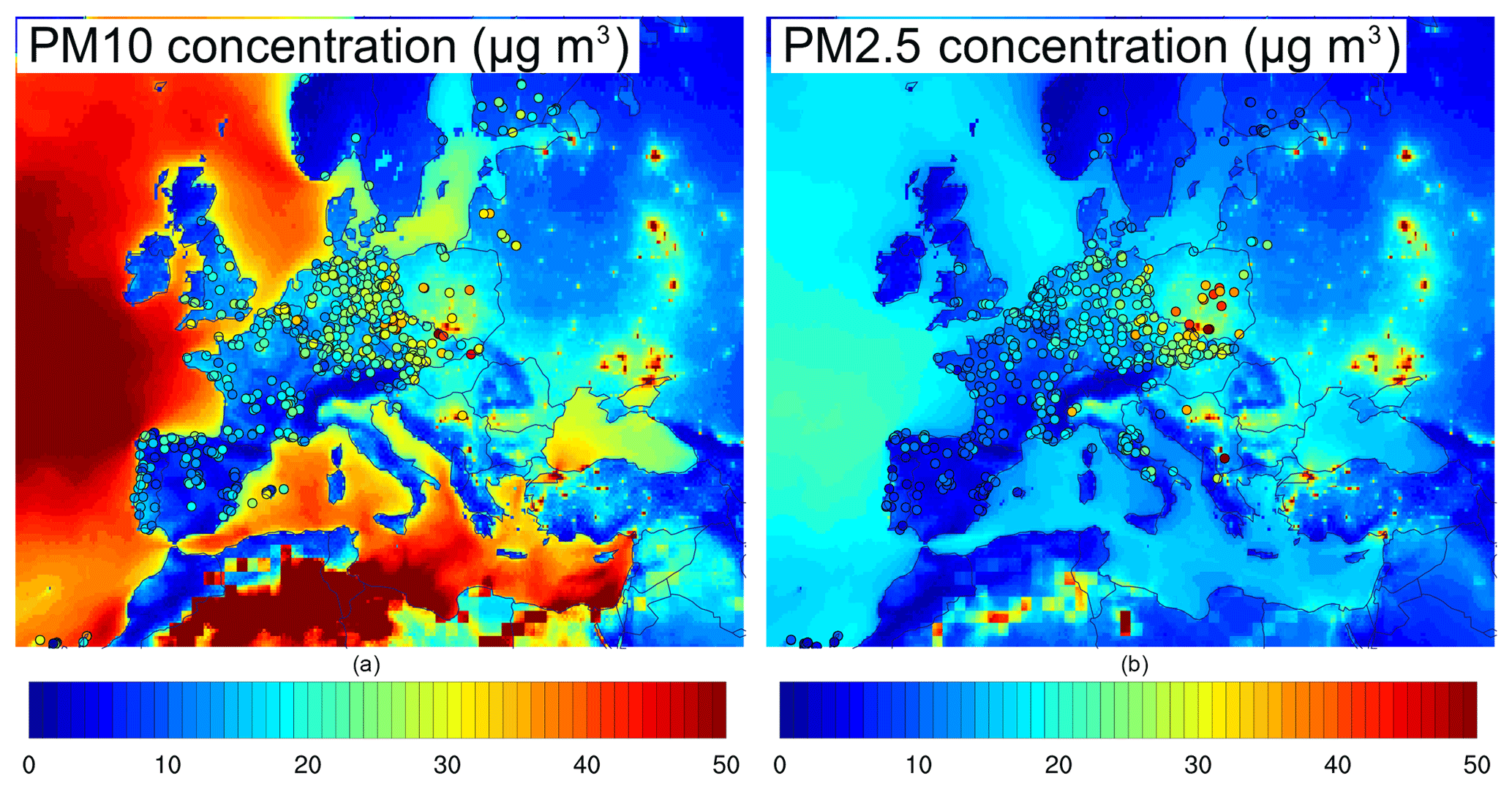
Figure 2 Mean PM₁₀ (a) and PM_2.5 (b) surface concentration (µg m⁻³) of the NR (shadings) and AQeR stations (colour circles) from January to April 2014.

The MOCAGE simulation covers the whole period from January to April 2014 on a global domain at 2^∘ resolution and in a nested regional domain, which covers Europe from 28 to 72^∘ N and from 26^∘ W to 46^∘ E, at 0.2^∘ resolution (see Fig. 2). A 4-month spin-up is made before the simulation. The NR is forced by ARPEGE meteorological analysis. Emissions of chemical species in the global domain come from the MACCity inventory (van der Werf et al., 2006; Lamarque et al., 2010; Granier et al., 2011) for anthropogenic gas species and biogenic species are from the Global Emissions InitiAtive (GEIA) for the global and regional domain. ACCMIP project emissions are used for anthropogenic organic and black carbon emissions on the global scale. The TNO-MACC-III inventory for the year 2011 provides anthropogenic emissions in the regional domain. TNO-MACC-III emissions are the latest update of the TNO-MACC inventory based on the methodology developed in the MACC-II project described in Kuenen et al. (2014). These anthropogenic emissions are completed in our regional domain, at the boundary of the MACC-III inventory domain by emissions from MACCity. Daily biomass burning sources of organic and black carbon and gases from the Global Fire Assimilation System (GFAS) (Kaiser et al., 2012) are injected in the model. The NR includes secondary organic aerosols (SOAs) in order to enhance its realism and to fit the observations made at ground-based stations over Europe well. Standard ratios from observations (Castro et al., 1999) are used to simulate the portion of secondary carbon species, with 40 % in winter from the primary carbon species in the emission input.

The NR is compared to the real observations from AERONET AOD observations and AQeR surface concentrations, using common statistical indicators: mean bias (B), modified normalized mean bias (MNMB), root mean square error (RMSE), fractional gross error (FGE), Pearson correlation coefficient (R_p) and Spearman correlation coefficient (R_s). While the Pearson correlation measures the linear relation between the two data sets, the Spearman correlation is a mean used to assess their monotonic relationship.

The AQeR stations are mainly located over western Europe (Fig. 2). After selection of the surface stations that are representative of background air pollution (following Joly and Peuch, 2012), 597 and 535 stations are respectively used for the PM₁₀–PM_2.5 comparison. Figure 2 represents the mean surface concentration of the NR and selected AQeR measurements over the domain from January to April 2014. The left panel shows the PM₁₀ concentrations of the NR in the background and the AQeR concentrations as a circle, while the right panel shows the PM_2.5 concentrations. The concentration of the NR PM₁₀ and PM_2.5 are generally underestimated compared to the observations. Nevertheless, in both figures, the spatial variability and, particularly, the location of maxima are reasonably well represented. Over the European continent, the NR and AQeR data show clear maxima in the centre of Europe for both PM₁₀ and PM_2.5 concentrations, even if the NR underestimates these maxima.

Table 1 Bias, RMSE, FGE, factor of 2, Pearson correlation (R_p) and Spearman correlation (R_s) of the NR simulation taking as reference the AQeR observations for hourly PM₁₀ and PM_2.5 concentrations from January to April 2014.

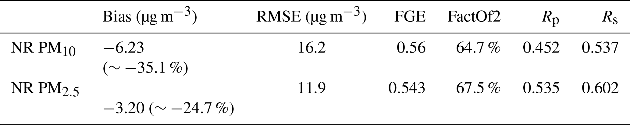
Table 1 shows the statistical indicators of this comparison for hourly surface concentrations in PM₁₀ and PM_2.5. A negative mean bias is observed, around −6.23 µg m⁻³ ($\sim -\mathrm{35.1}$ %) for PM₁₀ and −3.20 µg m⁻³ ($\sim -\mathrm{24.7}$ %) for PM_2.5. The RMSE is equal to 16.2 µg m⁻³ for PM₁₀ and 11.9 µg m⁻³ for PM_2.5, while the FGE equals 0.56 and 0.543. The factor of 2 is equal to 64.7 % and 67.5 % for PM₁₀ and PM_2.5. Pearson and Spearman correlations are respectively 0.452 and 0.535 for PM₁₀ and PM_2.5 and 0.537 and 0.602 for PM₁₀ and PM_2.5. The NR underestimation is greater for PM₁₀ than for PM_2.5 in relative differences. This suggests a lack of aerosol concentrations in the PM_10−2.5 (concentration of aerosols between 2.5 and 10 µm). Not taking into account wind-blown crustal aerosols may cause a potential underestimation of PM in the models (Im et al., 2015). Taking them into account requires a detailed ground-type inventory to compute those emissions unavailable in MOCAGE. For PM_2.5, the underestimation of aerosol concentrations can be due to a lack of carbonaceous species (Prank et al., 2016). Other possible reasons for the negative PM bias at the surface are the underestimation of emissions in the cold winter period and the uncertainty in the modelling of stable winter conditions with shallow surface layers.

Figure 3 Median of the daily mean surface concentration in µg m⁻³ of the NR (in purple) and the AQeR station (in black). The NR concentrations are calculated at the same locations as the AQeR stations from 1 January 2014 (Day 1) to 30 April 2014 (last day). The left panel is for PM₁₀ surface concentrations, while the right one is for PM_2.5.

A time-series graph of the median NR surface concentrations and the median surface concentrations of the AQeR stations are presented in Fig. 3. Compared to ground-based AQeR data (in black), the NR (in purple) generally underestimates the PM₁₀ and the PM_2.5 concentrations, especially during the 7–15 March pollution episode. However, the variations and maxima of the NR concentrations of PM are generally well represented. Furthermore, around 65 % of model concentrations are relatively close to the observations as shown by the factor of 2 in Table 1. The variability of NR concentrations is thus consistent with AQeR station concentrations.

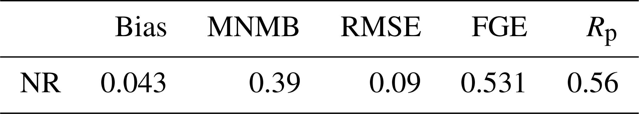
Table 2 gives an evaluation of the NR against the daily mean of the AOD at 500 nm obtained from 84 AERONET stations in the regional domain from January to April 2014. The statistical indicators show good consistency between the NR and AERONET observations. However, like the results shown on a global scale (Sič et al., 2015), MOCAGE tends to overestimate AOD: although small, the AOD bias is positive. While PM concentrations at the surface are underestimated in the NR, there may be different reasons for an overestimation of AOD. The vertical distribution of aerosol concentrations in the model is largely controlled by vertical transport, removal processes and by the prior assumptions on the aerosol emission profiles. However, these processes may have large variability and they are prone to large uncertainties (Sič et al., 2015). Another possible explanation is the uncertainty of the size distribution of aerosols that can significantly affect the optical properties. More generally, the assumptions that underly the computation of optical properties are largely uncertain and they can affect the computation of AOD by a factor of 50 % (Curci et al., 2015): the mixing state assumption, and the uncertainty in refractive indices and in hygroscopicity growth. These uncertainties in aerosol vertical profiles, size distribution and optical properties may explain the decorrelation between AOD and PM concentrations at the surface and why the MOCAGE NR has a positive bias in AOD while underestimating PM at the surface. However, both the PM and AOD correlation errors of the NR remain in a realistic range.

Table 2 Bias, MNMB, RMSE, FGE and Pearson correlation (R_p) between the NR simulation and AERONET station for daily 500 nm AOD from January to April 2014.

As a result, the NR simulation exhibits surface concentrations and AODs in the same range compared to those from ground-based stations and shows similar spatial and temporal variations, which makes the NR acceptable for the OSSE.

3 Generation of synthetic AOD observations

The study focuses on the added value of assimilating AODs at the central wavelength (444 nm) of the FCI/VIS04 spectral band. Since the assimilation of AODs from several wavelengths simultaneously is not possible (Sect. 2.3), the choice of the single-channel VIS04 is mainly driven by the fact that it is the shortest wavelength of FCI, which is a priori the most favourable for the detection of fine particles.

Thus, synthetic AOD observations at 444 nm are created over the MOCAGE-simulated regional domain from the NR simulation 3-D fields: all aerosol concentrations per type and per size bins, and meteorological variables. At every grid point of the NR regional domain where the solar zenith angle is below 80^∘ (daytime) and where clouds are absent, an AOD value at 444 nm is computed using the MOCAGE observation operator described above (Sect. 2.3). In order to take into account the error characteristics of the FCI VIS04 AOD, a random noise is then added to this NR AOD value.

To estimate the variance of this random noise, the general principle is to assess and quantify the respective sensitivity of the FCI VIS04 top-of-the-atmosphere reflectance to AOD and to the other variables. To do this, the FCI simulator developed by Aoun et al. (2016), based on the radiative transfer model (RTM) libRadtran (Mayer and Killings, 2005), has been used. This simulator computes the reflectance in the different spectral bands of FCI as a function of different input atmospheric parameters (AOD τ, total column water vapour, ozone content), ground albedo ρ_g and solar zenith angle θ_S, for different OPAC (optical properties of aerosols and clouds, Hess et al., 1998) aerosol types: dust, maritime clean, maritime polluted, continental clean, continental average, continental polluted and urban. The FCI simulator takes into account the spectral response sensitivity and the measurement noise representative of the FCI VIS04 spectral band (415–475 nm).

Table 3 Conditions for classifying the MOCAGE NR into the OPAC types. The first condition is the surface concentrations, the second is the main specie at the surface between desert dust (DD), sea salt (SS) and IWS (insoluble, water soluble and soot) and the third is a condition of the species over all the aerosol concentrations. A species is described as a main species if its concentrations is above all other concentrations; for example DD is a main species if [DD] > [SS] and [DD] > [IWS].

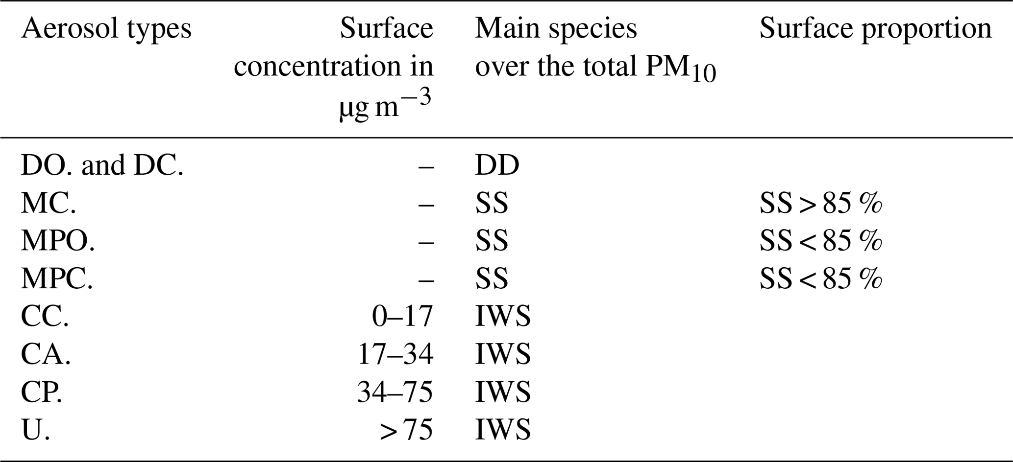
By applying a global sensitivity analysis to this FCI simulator that was run on a large data set (see the Appendix for the details of the method), a look-up table of the RMSE of AOD is derived. It depends on the OPAC type, the relative error of surface albedo, the solar zenith angle and the ground albedo value. The classification of each MOCAGE profile into the OPAC types relies on three parameters (Table 3): the surface concentration, the main surface species and the proportion in relation to the total aerosol concentrations. A species is described as a main species if its concentration, [species], is above the concentration of all other types of aerosol. For example DD is a main species if [DD] > [SS] and [DD] > [IWS]. An example of NR profiles (7 March 2014 at 12:00 UTC) decomposed in OPAC type is presented in Fig. 4. A small number of the profiles are dismissed where MOCAGE profiles do not match one of the OPAC types, such as profiles over ocean where IWS (insoluble, water soluble and soot; Table 3) is greater than DD (desert dust) and SS (sea salt). A larger number of profiles are dismissed because of night-time profiles and cloudy conditions. Figure 5 represents the average number of NR AODs that are retained per day for assimilation. After these filters apply, between 10 % and 20 % of profiles are kept every hour. The density of these profiles is higher in the south of the domain, which is directly correlated to the quantity of direct sunlight available. Over the continent, between 1 and 4 profiles can be assimilated per day at each grid-box location.

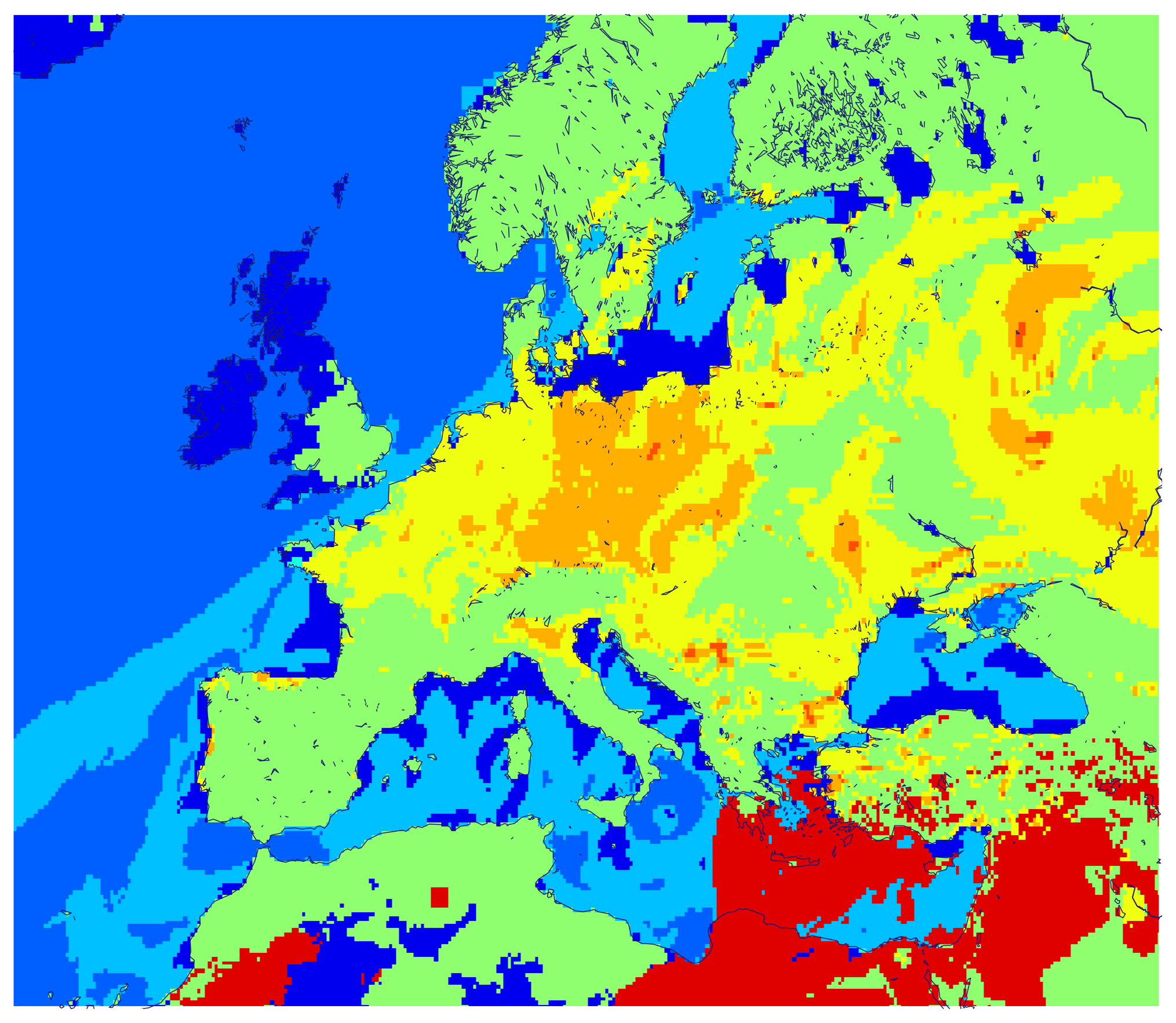
Figure 4 Classification of the NR profiles for the 7 March 2014 at 12:00 UTC. Deep blue is for dismissed profiles, blue is for maritime clean, light blue for maritime polluted, green is for continental clean, yellow is for continental 5 average, orange is for continental polluted, deep orange is for urban, and red is for desert dust.

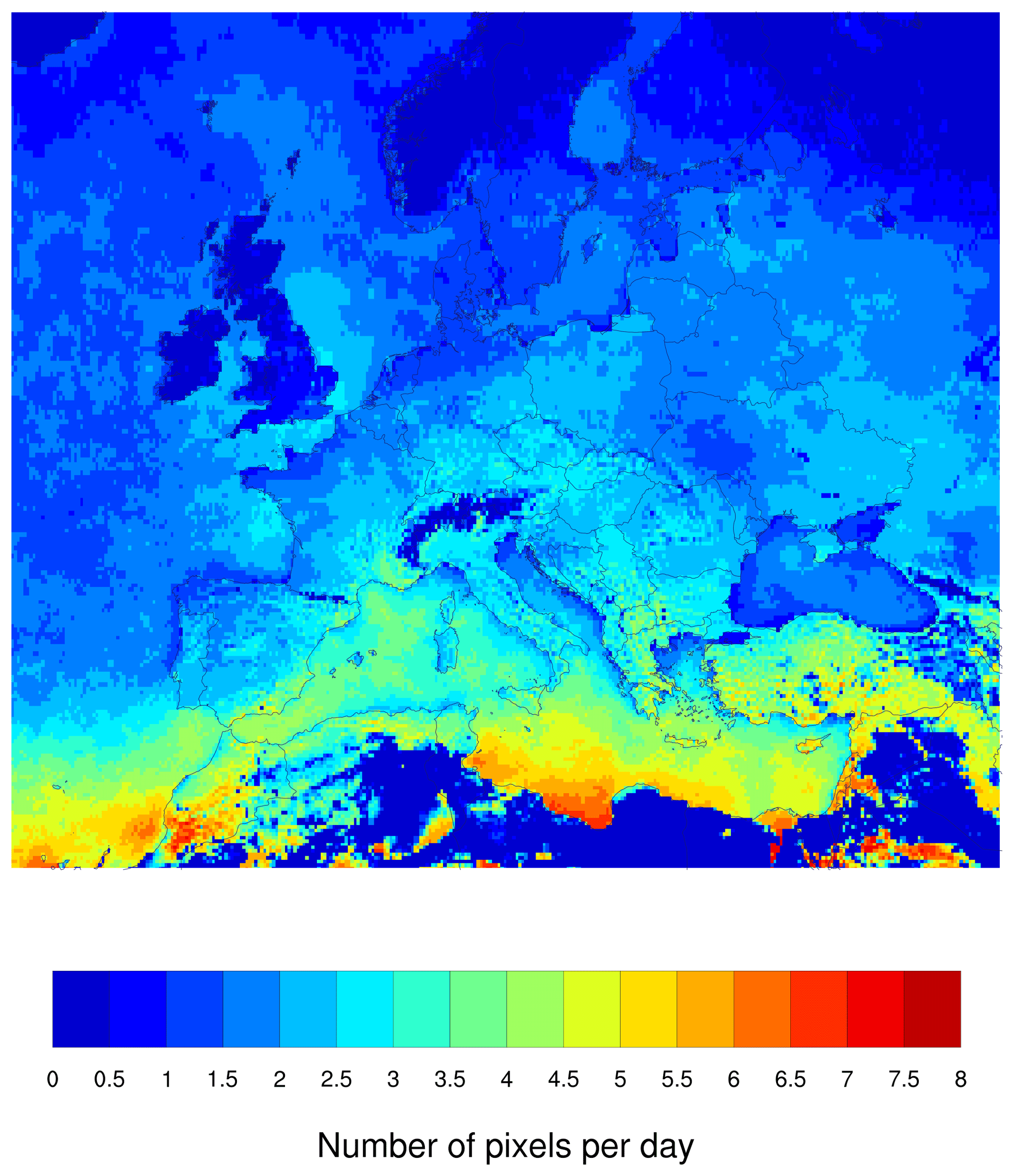
Figure 5 Average (from January to April) number of selected profiles per day available for assimilation.

On every NR profiles that is kept, an AOD error is introduced, by addition of a random value from an unbiased Gaussian with a standard deviation derived from the AOD RMSE look-up table, calculated as explained above. The surface albedo fields are taken from MODIS using the radiative transfer model RTTOV (Vidot et al., 2014). A relative error of 10 % is assumed for ground albedo, which corresponds to a realistic value (Vidot et al., 2014). An example of the synthetic observations is presented in Fig. 6. It represents the NR AOD, the synthetic observations and the noise applied to NR AOD for the 7 March 2014 at 12:00 UTC.

4 Controls runs (CRs) and their comparison to NR

Section 2 showed an evaluation of the NR compared to real observations. Another requirement of the OSSE is the evaluation of differences between the NR and the CR. Various CR simulations have been performed to evaluate the behaviour of the OSSE in different CR configurations and prove its robustness. The NR and CRs use different set-ups of MOCAGE. The CRs use IFS meteorological forcings, while the NR uses ARPEGE meteorological forcings. The use of different meteorological inputs is expected to yield differences in the transport of pollutant species, and changes in dynamic emissions of sea salt and desert dust. To introduce more differences between the CRs and NR, changes in the emissions are also introduced.

Figure 6 Example of generation of synthetic observations on the 7 March 2014 at 12:00 UTC. From the NR AOD as 444 nm (a), noise values representative of FCI (b) are applied to every clear-sky pixel to generate the synthetic observations (c). The grey colour represents the dismissed profiles.

Table 4 indicates the changes made to the different model parameters to create four distinct CR simulations. The first control run, CR1, uses the same inputs as the NR except for the meteorological forcings. Other control runs (CR2, CR3, CR4) do not have the SOA formation process of the NR (Sect. 2) and CR1 simulations. Finally, CR3 and CR4 change from other simulations by different vertical repartitions of emissions in the five lowest levels. In CR3, the pollutants are emitted with a slower decay with height than the NR (with repartition from 30 % at the surface and respectively 24 %; 19 %; 15 %; 12 % for the four levels above), and in the CR4 emissions are only injected in the lowest level. These changes aim to generate simulations that are more significantly different from the NR than the first two control runs.

Table 4 Table of differences between the NR simulation and the CR simulations.

The four CRs are compared to the NR for PM₁₀ and PM_2.5 surface concentration considering virtual observations at the same locations as the AQeR stations. A time series of daily means of surface concentrations at simulated stations is presented in Fig. 7 for NR and CR simulations from 1 January to 30 April 2014. The PM₁₀ concentrations of the NR (in purple) are mostly greater than the PM₁₀ concentrations in the CRs. During the period of late March and early April (around the 90th day of simulation) the NR concentrations of PM₁₀ are close to those of the CR2, CR3 and CR4, and less than those of the CR1 by about a few µg m⁻³. In terms of PM_2.5, the CR concentrations also underestimate the NR concentration. As for PM₁₀, around the 90th day of simulation, the concentrations of CR1 are above the concentrations of the NR.

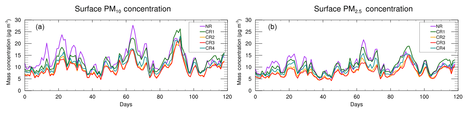
Figure 7 Median of the daily mean surface concentration of the NR (in purple) and the different CRs (CR1 in green, CR2 in yellow, CR3 in red and CR4 in blue) determined for the same location as for the AQeR stations. Panel (a) is the PM₁₀ mass concentration (µg m⁻³), while (b) represents the PM_2.5 mass concentrations.

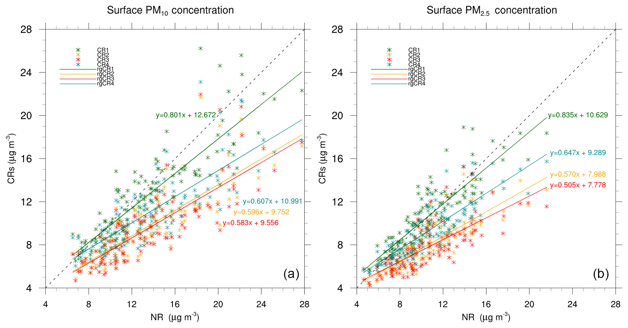
Figure 8 Scatter plot of the CR daily surface concentrations (µg m⁻³) as a function of NR daily surface concentrations for PM₁₀ (a) and PM_2.5 (b), for virtual stations and from January to April 2014. rgCRX are the linear regressions of each data set.

These tendencies can also be observed in Fig. 8, which represents a scatter plot of CR concentrations as a function of NR concentrations for the daily means of surface concentration in PM₁₀ and PM_2.5 at the virtual stations. The CR1 concentrations are fairly close to those of the NR concentrations with a coefficient of regression about 0.801 and 0.835 for PM₁₀ and PM_2.5. Other CRs underestimate the NR concentrations. This tendency is stronger for PM₁₀ than for PM_2.5. The regression coefficients of the CR2, CR3 and CR4 are respectively 0.596, 0.583 and 0.607 for PM₁₀ and 0.570, 0.505 and 0.647 for PM_2.5. For both PM₁₀ and PM_2.5 concentrations, the underestimation is more important for high values of the NR concentrations than for low values.

The statistical indicators in Tables 5 and 6 are consistent with Figs. 7 and 8. The CR1 is close to the NR with a bias of −1.3 µg m⁻³ (−8.2 %) for PM₁₀ and −0.8 µg m⁻³ (−6.2 %) for PM_2.5. The CR4 bias is around −2.9 µg m⁻³ (−20.5 %) for PM₁₀ and −1.8 µg m⁻³ (−15.1 %) for PM_2.5. The two other CRs highly underestimate PM₁₀ and PM_2.5 concentrations with biases of −4.5 µg m⁻³ (−35.2 %) and −3.9 µg m⁻³ (−37.4 %) respectively for CR2 and −4.8 µg m⁻³ (−38.1 %) and −4.4 µg m⁻³ (−42.6 %) for the CR3. These biases are in agreement with the literature. Prank et al. (2016) measure a bias around −5.8 for PM₁₀ and −4.4 µg m⁻³ for PM_2.5 for the median of four CTMs against ground-based stations in winter. In Marécal et al. (2015), statistical indicators for an ensemble of seven models are presented for winter. A bias between −3 and −7 µg m⁻³ is observed for the median ensemble. The PM concentrations of our CRs compared to the NR are characteristic of models compared to observations.

Table 5 Bias, RMSE, FGE, factor of 2, Pearson correlation (R_p) and Spearman correlation (R_s) of the CR simulation taking as reference the NR simulations for hourly PM₁₀ concentrations from January to April 2014. The comparison is made at the same station location as for AQeR stations.

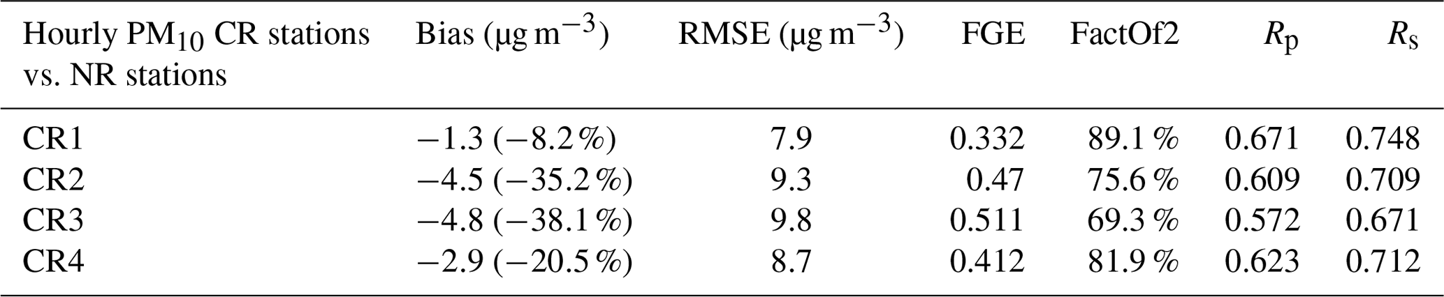
Table 6 Bias, RMSE, FGE, factor of 2, Pearson correlation (R_p) and Spearman correlation (R_s) of the CR simulation taking as reference the NR simulations for hourly PM_2.5 concentrations from January to April 2014. The comparison is made at the same station location as for AQeR stations.

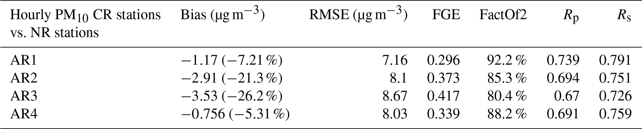
Table 7 Bias, RMSE, FGE, factor of 2, Pearson correlation and Spearman correlation of the ARs simulation taking as reference the NR simulations for hourly PM₁₀ concentrations from January to April 2014. The comparison is made at the same station location as for AQeR stations.

Prank et al. (2016) also show other indicators of the median of models, such as the temporal correlation and the factor of 2. Their correlations are around 0.7 for PM_2.5 and 0.6 for PM₁₀ and are close to those for our CR simulations that vary from 0.644 to 0.732 for PM_2.5 and from 0.572 to 0.671 for PM₁₀. Their factor of 2 equals 65 % for PM₁₀ and 67 % for PM_2.5. The factor of 2 of the CRs ranges between 70 % and 90 % for both PM₁₀ and PM_2.5 concentrations. The RMSE of CR simulations ranges from 8 to 10 µg m⁻³ for PM₁₀ concentrations, which is slightly under the RMSE of the ensemble from the study of Marécal et al. (2015), which ranges between 10 and 15 µg m⁻³. The FGE of the study of Marécal et al. is equal to 0.55, while the FGE of CRs varies from 0.33 to 0.51. Our CR simulations slightly underestimate the model relative error. Thus, compared to the literature, the CRs (especially the CR3) are different enough from the NR to be representative of state-of-the-art simulations.

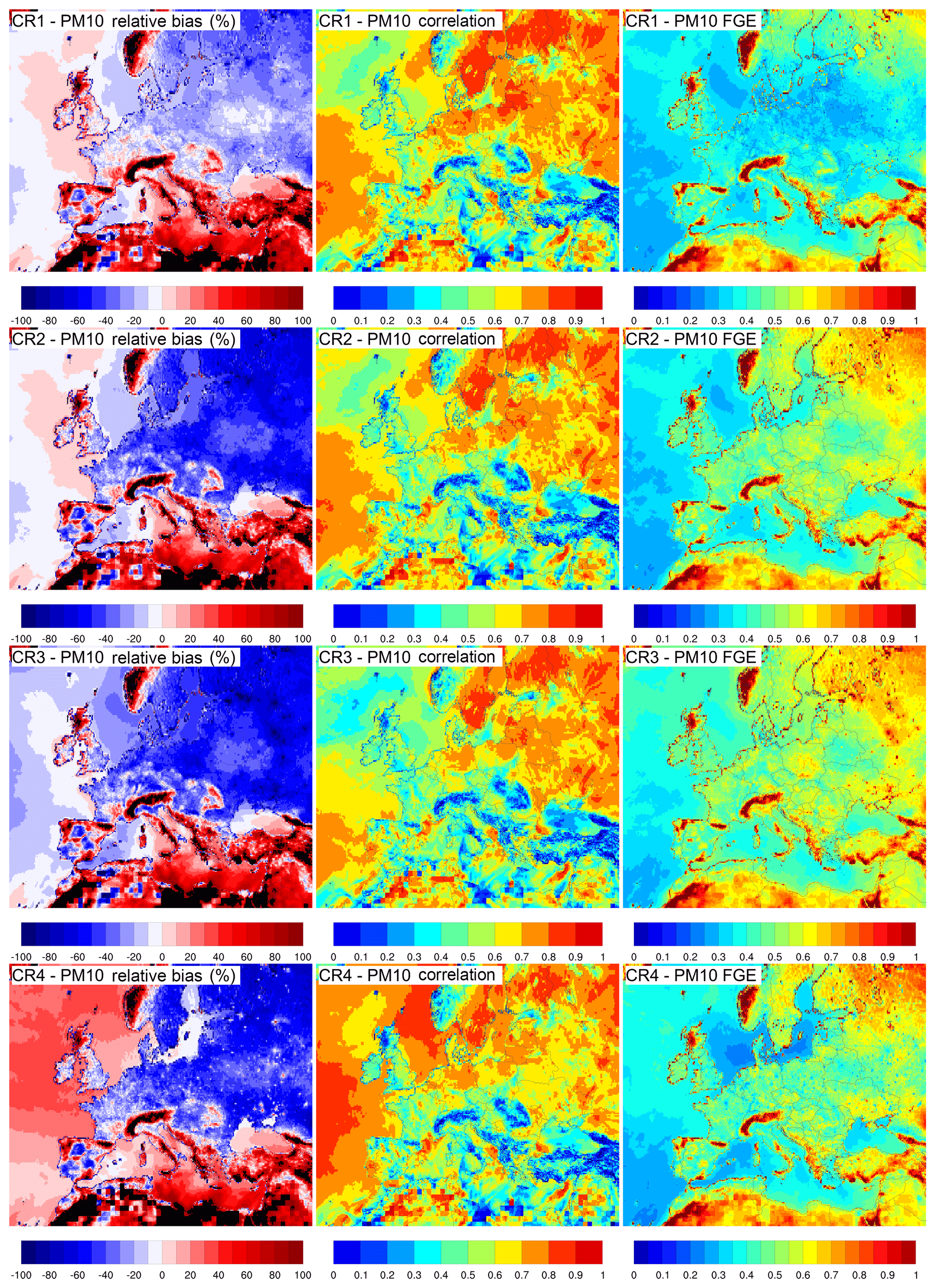
Figure 9 For each CR (CR1, CR2, CR3 and CR4), the figures represent a PM₁₀ comparison between the NR and the CRs from January to April 2014: the relative bias (in %), the Pearson correlation and the fractional gross error.

Between the CRs and the NR there are important spatial differences in the surface concentrations of PM, as demonstrated in Fig. 9, which shows the relative differences, Pearson correlation and the FGE for PM₁₀. Over the Atlantic Ocean, the CR concentrations are relatively close to the NR, except for the CR4 which overestimates the concentration of PM₁₀. All CRs present high concentrations of PM₁₀ all over northern Africa. This corresponds to high emissions of desert dust over this area, which cause an important overestimation of PM₁₀ compared to the NR. This overestimation can be observed around all the Mediterranean Basin. The CRs tend to overestimate the PM₁₀ concentrations over Spain, Italy, the Alps, Greece, Turkey, the north of the UK, Iceland and Norway. The overestimations over the Alps, Iceland and Norway are located at places of negligible concentrations. Over the rest of the European continent, CRs underestimate the concentration of PM₁₀, slightly for CR1, but concentrations are very pronounced for CR2, CR3 and CR4. The area where the consistency between the CRs and the NR is better is the Atlantic Ocean, with a correlation ranging from 0.6 to 0.9 and a low FGE around 0.3. Over the Mediterranean Basin the correlation varies significantly between 0 and 1. Low correlations correspond to high FGE around 1. Over the continent, the correlation varies from 0.4 to 0.9, following a west–east axis. The correlations are slightly greater for CR1 than for the other CRs. The FGE over the continent changes significantly for CR1 and the other CRs, respectively around 0.35 and 0.55. Similar conclusions can be obtained for the PM_2.5 comparison (see Supplement). A similar comparison has been done for the AOD between the CR simulations and the NR simulation (see complementary materials).

In summary, the control runs present spatial variability along with temporal variability. The closest CR to the NR is the CR1. In terms of surface concentrations in PM, the CR3 is the most distant, while in terms of AOD the CR4 is the most distant. Those differences and the use of different CRs, coupled with the realism of the NR, demonstrate the robustness of the OSSE to evaluate the added value provided by AOD derived from the FCI.

5 Assimilation of FCI synthetic observations

The purpose of this paper is to assess the potential contribution of the FCI VIS04 channel to the assimilation of aerosols on a continental scale. In our OSSE, MOCAGE represents the atmosphere with a horizontal resolution of 0.2^∘ (around 20 km at the equator). Synthetic observations are therefore computed at the model resolution, although FCI scans around 1 km resolution at the equator and 2 km over Europe. To fit with the time step of our assimilation cycle, synthetic observations are also created every hour, although the future FCI imager could retrieve radiance observations every 10 min over the globe, and 2.5 min over Europe with the European Regional-Rapid-Scan. This means that, for each profile of our simulation, only one synthetic observation is available each hour, instead of $\mathrm{24}\times \mathrm{10}\times \mathrm{10}$ at best (FCI scans 24 times an hour, with a spatial resolution 10 times higher than the model over the Europe). The use of one observation for each profile in an assimilation window is due to the assimilation system design that does not allow multiple observations for the same profile. In practice, future FCI observations could be averaged over each MOCAGE profile to reduce the impact of the instrument errors on assimilated observations.

The 3D-FGAT assimilation scheme integrates the synthetic observations described in Sect. 3. Before assimilation, a thinning process is applied to the synthetic observations to spatially keep only 1 pixel out of 4. Such thinning is useful for reducing the computation time, by accelerating the convergence of the cost function (not shown). The spatial correlation length of the B background covariance matrix is set to 0.4^∘ in order to have a spatial impact of the assimilation on the simulation while not having multiple coverage of assimilated observations over one profile. The result of this thinning procedure changes the assimilated fields only slightly but significantly saves computing time. Assimilation simulations (ARs) are run for all CR simulations using the same generated set of synthetic observations over the period of 4 months, from 1 January to 30 April. The standard deviation of errors used for B and R matrices are estimated respectively at 24 % and 12 %, as in Sič et al. (2016).

To assess the impact of the assimilation of FCI synthetic AOD observations, the CR forecasts and the AR analyses are compared to the assimilated synthetic observations. Figure 10 shows the histograms of the differences between the synthetic observations and the forecast field (in blue) and between synthetic observations and analysed fields (in purple) for the four ARs simulations. The histograms follow a Gaussian shape, and the distribution of the analysed values are closer to the synthetic observations than the forecast values. The spread of the histograms is smaller for the analysed fields than for the forecast fields. The assimilation of synthetic AODs hence improved the representation of AOD fields in the assimilation simulations. Besides, the spatial comparisons between the simulations and the NR show improvements in the AOD fields of simulations by assimilation of the synthetic observations (see Supplement Figs. S5, S6, S7 and S8). As the increment is applied to all aerosol bins and PM₁₀ corresponds to 5 of the 6 bins while PM_2.5 to only 4, we expect better corrections for PM₁₀ concentrations than for PM_2.5 concentrations.

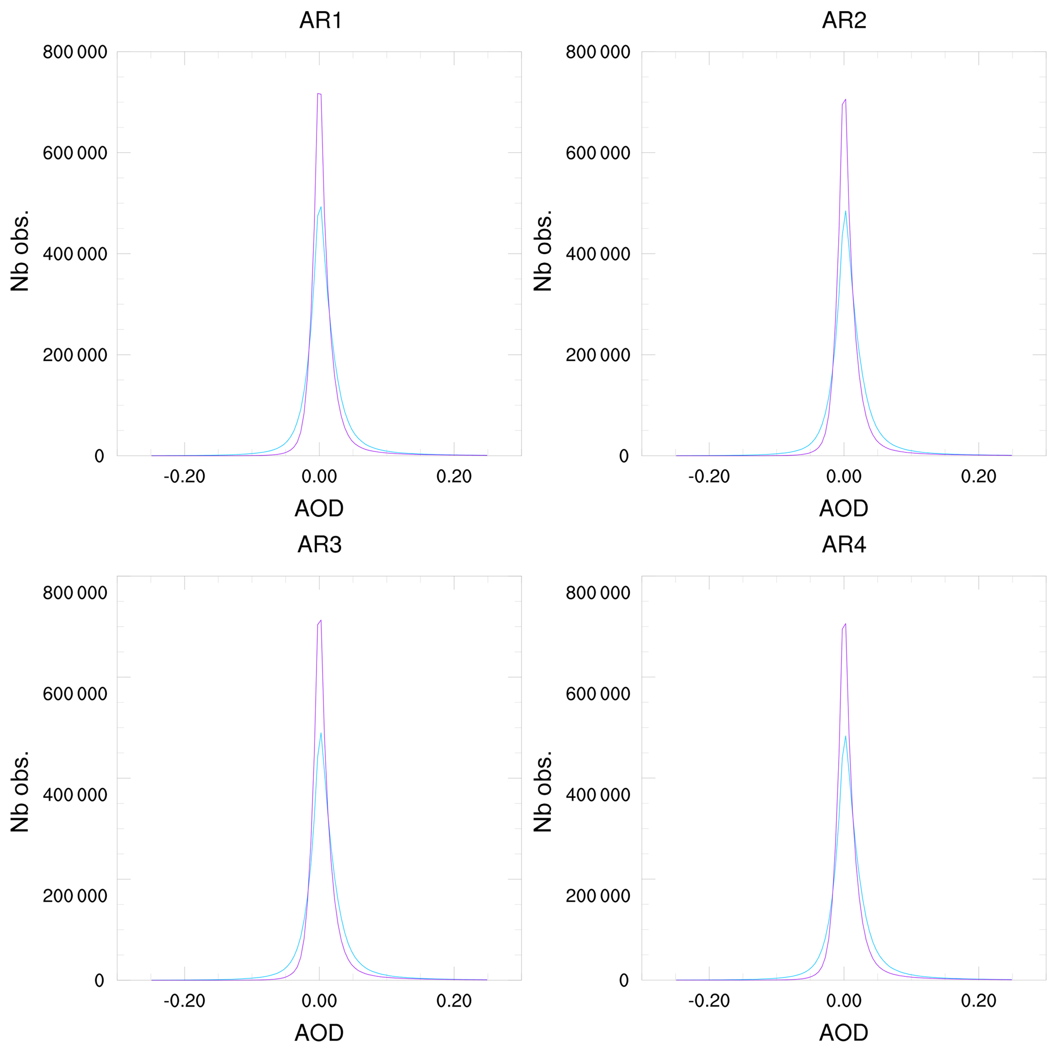
Figure 10 Histograms of differences between synthetic observations and forecast fields (blue) and between synthetic observations and analysed fields (purple) for the four assimilation runs.

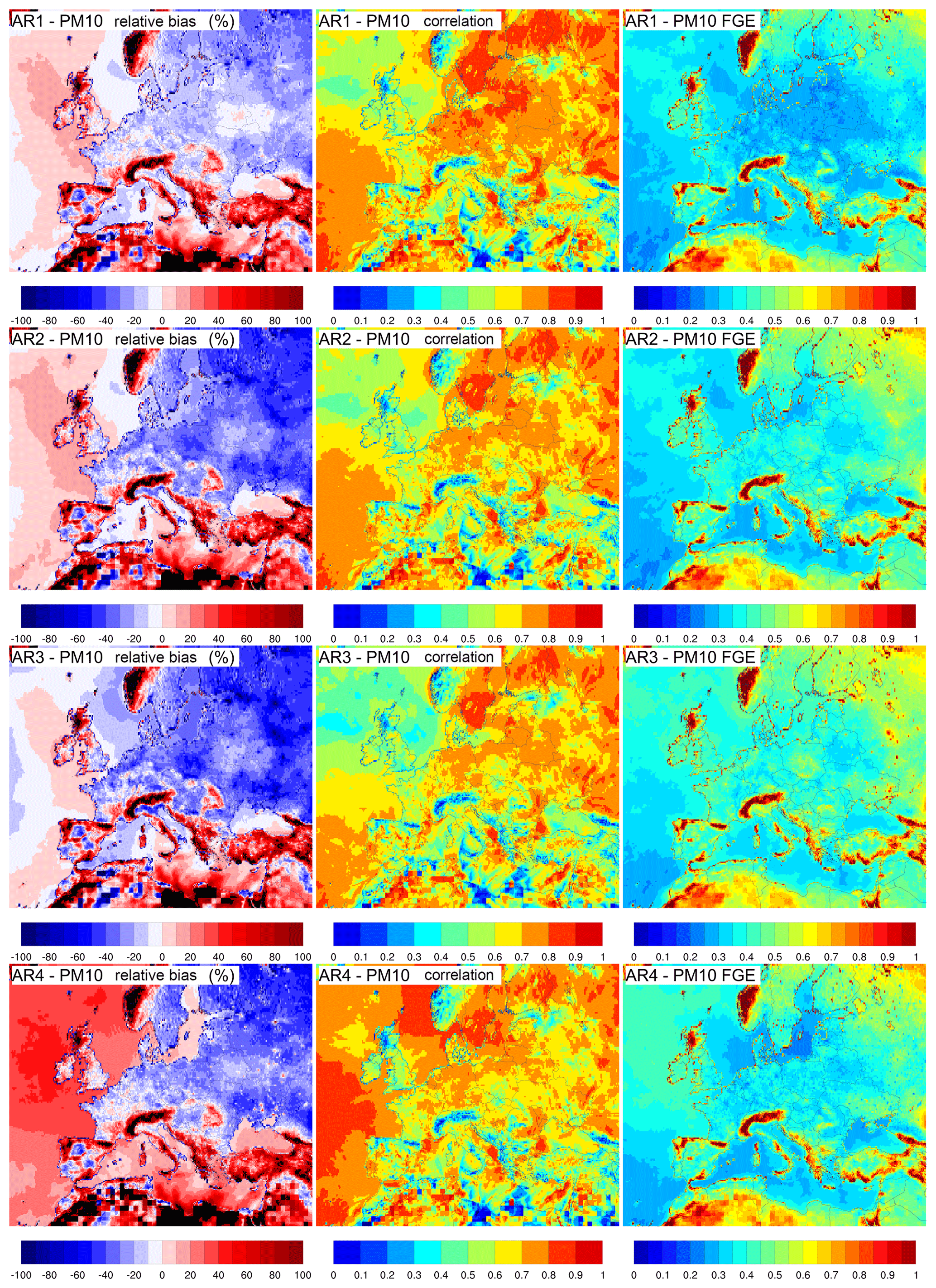
Figure 11 Same legend as Fig. 9, but for assimilation runs (AR) instead of control runs (CR).

To validate the results of the OSSEs, the simulations are compared to the reference simulation (NR) over the period. Figure 11 exhibits the spatial differences in the surface concentrations of PM₁₀ between the ARs and the NR. It shows the mean relative bias, the correlation and the FGE for every simulation. Using Fig. 9 as a reference, the relative bias, the FGE and the correlation have been improved over most parts of the domain after assimilation for all simulations. Over the European continent, all simulations show a strong improvement of the statistical indicators. For instance in CR3, along a line that goes from Spain to Poland, the FGE decreases by about 0.1 after assimilation. In the eastern part of Europe (from Turkey to Finland), the decrease in FGE is even higher. Over northern Africa and the Mediterranean Sea the improvement is intermediate. Nevertheless, the mean bias over the ocean tends to increase for the simulations, especially for AR4. This can also be observed for the PM_2.5 concentration comparison (see Figs. S1, S2, S3 and S4).

Table 8 Bias, RMSE, FGE, factor of 2, Pearson correlation and Spearman correlation of the ARs simulation taking as reference the NR simulations for hourly PM_2.5 concentrations from January to April 2014. The comparison is made at the same station location as for AQeR stations.

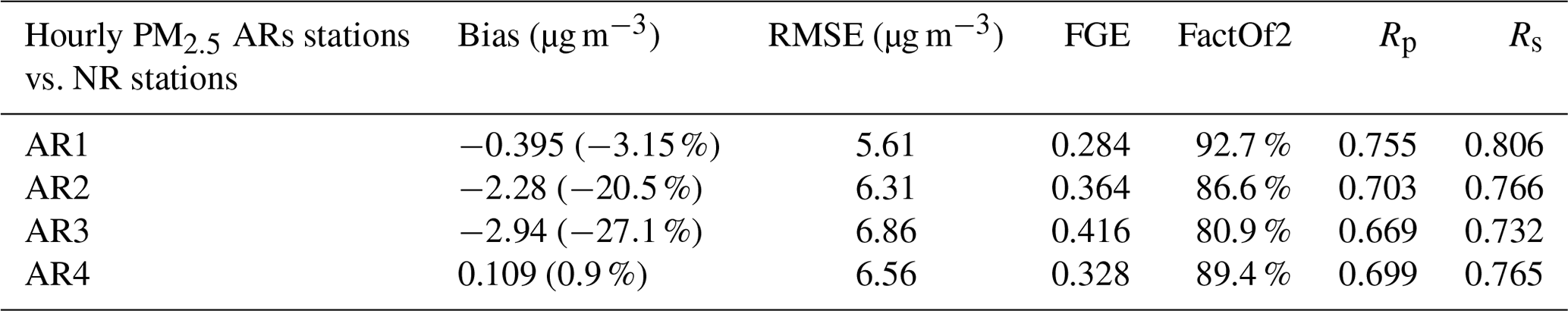
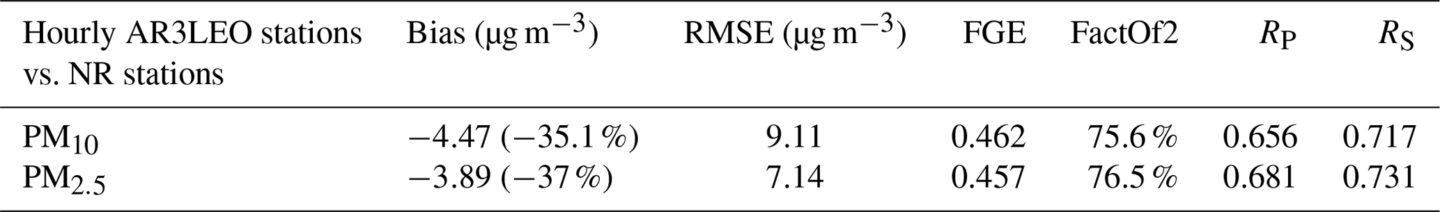
Table 9 Bias, RMSE, FGE, factor of 2, Pearson correlation and Spearman correlation of the AR3LEO simulation taking as reference the NR simulations for hourly PM₁₀ and PM_2.5 concentrations from January to April 2014. The comparison is made at the same station location as for AQeR stations.

The assimilation of the synthetic observations has a positive impact at each layer of the model. The mean vertical concentrations of PM₁₀ and PM_2.5 of the different simulations are represented in Figs. 12 and 13, from the surface (level 47) up to 6 km (level 30). The positive impact along the vertical of the assimilation of AODs in the CTM MOCAGE is due to the use of the vertical representation of the model to distribute the increment. Sič et al. (2016) showed that the assumption of using the vertical representation of the model gives good assimilation results with the regular MOCAGE set-up, which distributes emissions over the five lowest vertical levels. However, the performance of the assimilation may depend on the realism of the representation of aerosols along the vertical in the CTM. The CR simulations, in red, overestimate the PM₁₀ concentrations of the NR, in purple, due to the overestimation of desert dust concentrations in the CR simulations. This overestimation is not present in the PM_2.5 concentrations because this is the fraction of aerosols in which there is little desert dust. For the first three simulations, the vertical PM₁₀ concentrations are corrected well by the assimilation, while for simulation 4, the correction is less relevant for the levels near the surface. The assimilation tends to decrease the PM_2.5 concentrations above level 42 and to increase the concentrations under that level. Simulation 4 presents a decay of the surface concentrations of PM_2.5. The correction of concentrations is more pertinent for the PM₁₀ concentrations than for the PM_2.5 concentrations, which was expected.

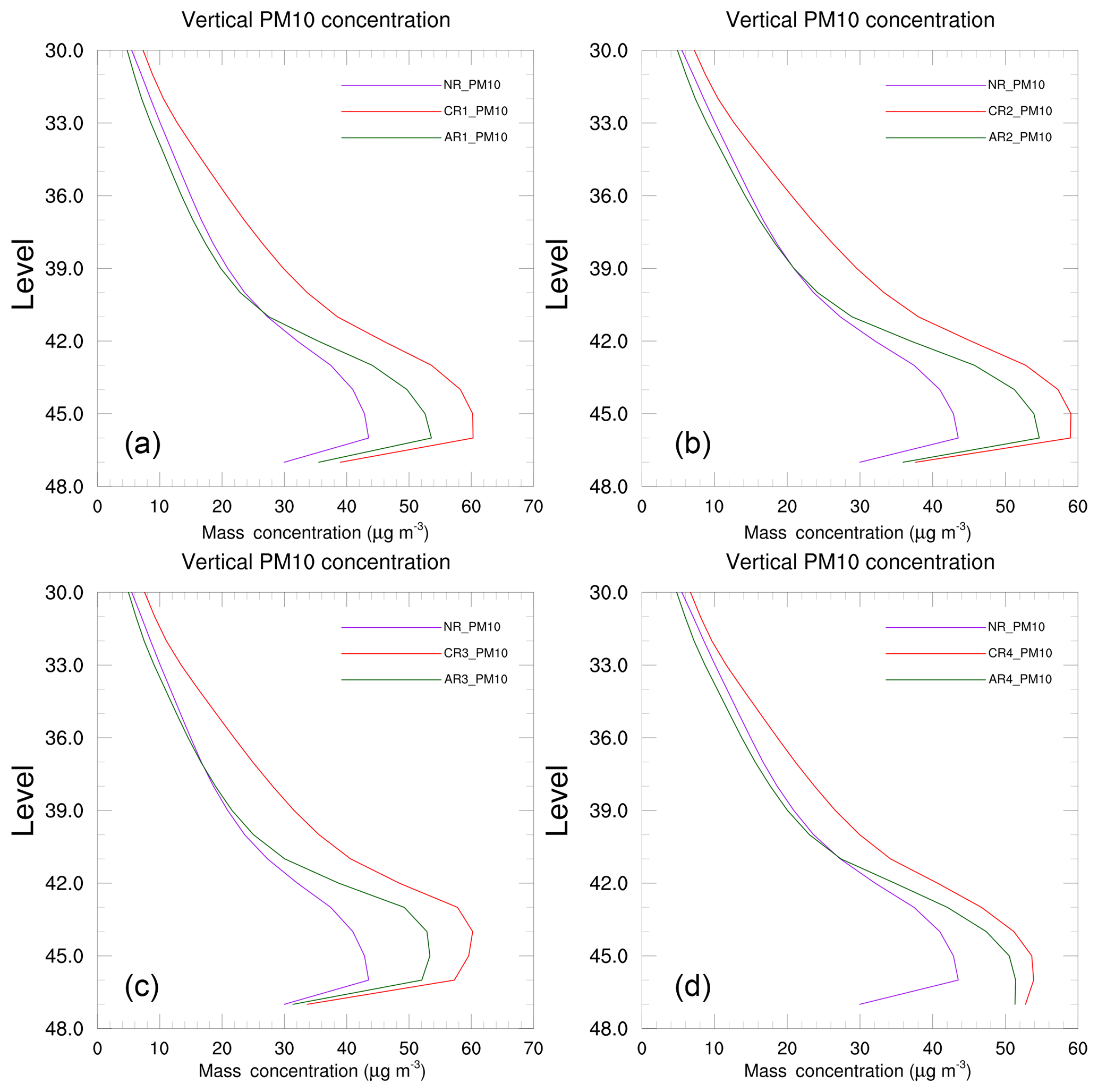
Figure 12 Mean vertical profile from January to April over the domain of the concentrations (µg m⁻³) of PM₁₀ for the four sets of simulations (1 in a, 2 in b, 3 in c and 4 in d). The NR is in purple, the CR is in red and the AR is in green.

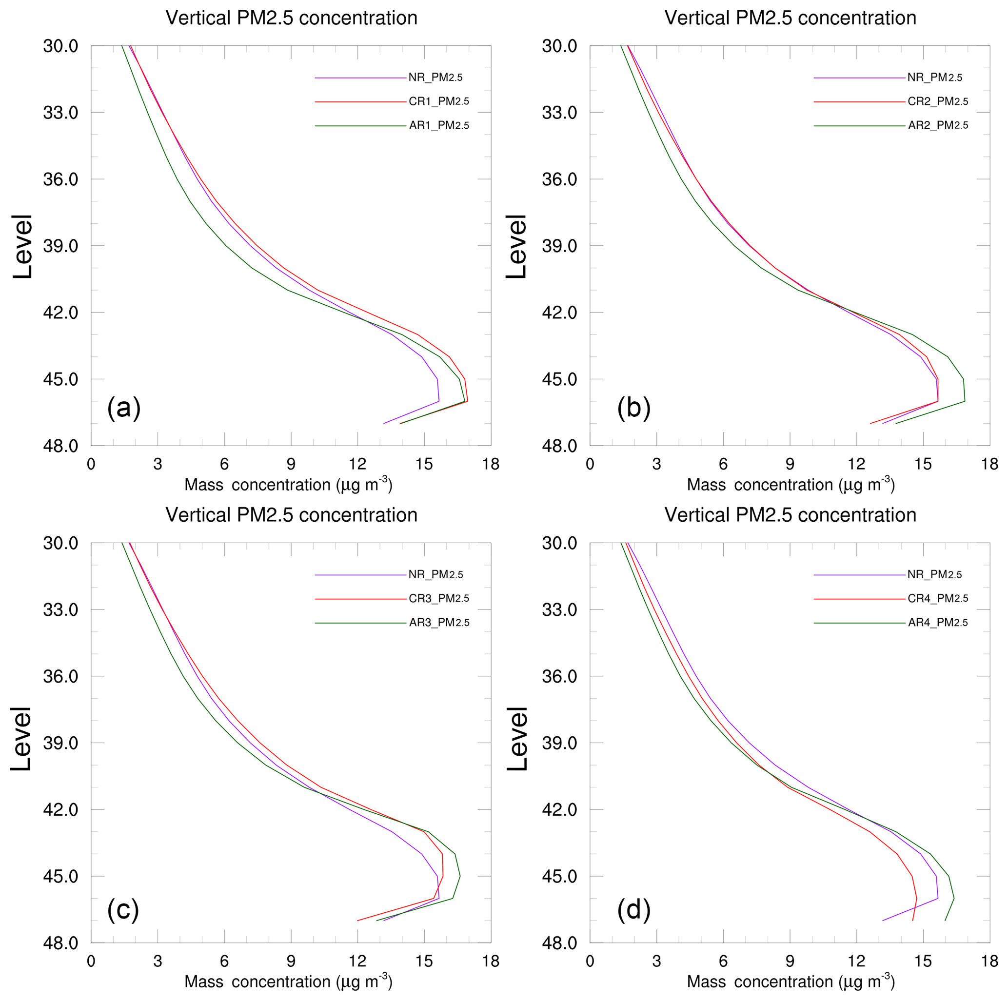
Figure 13 Mean vertical profile from January to April over the domain of the concentrations (µg m⁻³) of PM_2.5 for the four sets of simulations (1 in a, 2 in b, 3 in c and 4 in d). The NR is in purple, the CR is in red and the AR is in green.

In AR4, the PM₁₀ bias over the Atlantic Ocean is positive and larger than in CR4: the assimilation of FCI AODs can be detrimental in some circumstances. A reason for such deficiencies is proposed. In CR4, the AOD bias is negative (see Supplement) but the PM₁₀ bias is positive (Fig. 9) due to a vertical distribution of emissions limited to the lowest MOCAGE level. As a result of the assimilation, the aerosol increments associated with the synthetic AOD observations are positive and they are responsible for increasing the PM₁₀ fields at the surface. In the other CRs, the AOD bias over the Atlantic is mostly negative, as the PM bias, and the ARs are better than the corresponding CRs. In other words, where the surface PM bias and the AOD bias do not have the same sign, the assimilation of AODs can be detrimental.

To evaluate the capability of the FCI 444 nm channel observations to improve aerosol forecast in an air quality scenario, the AR simulations have been compared to the NR using the synthetic AQeR stations as in Sect. 4. Tables 7 and 8 show the statistics of the comparison between the ARs and the NR for PM₁₀ and PM_2.5 concentrations. With regard to the comparison of the CRs against the NR in Tables 5 and 6, the ARs are more consistent with the NR. The bias is reduced for both PM₁₀ and PM_2.5 concentrations. The RMSE and the FGE decrease, while the factor of 2 and the correlations increase for all ARs compared to their respective CRs.

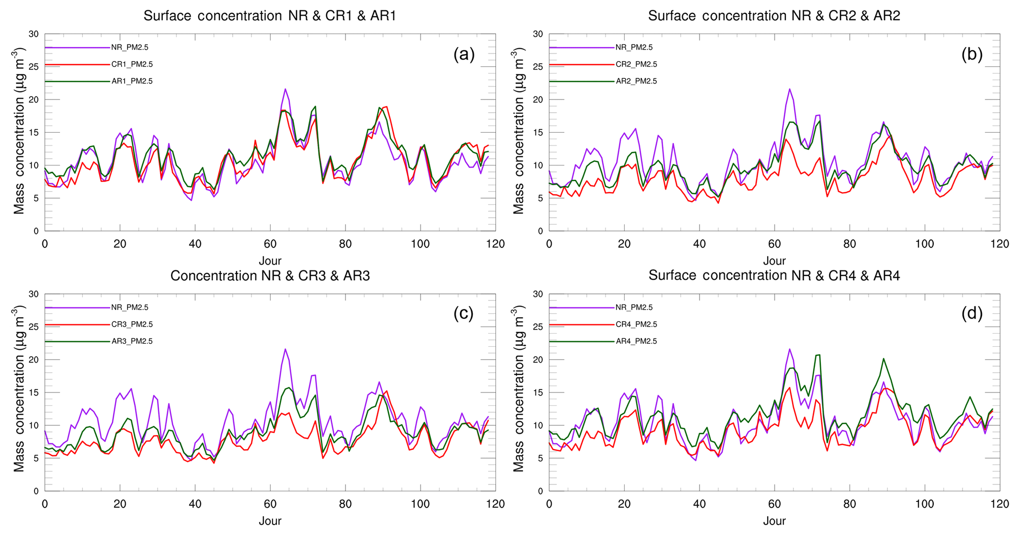
The daily medians of PM₁₀ and PM_2.5 concentrations at all stations are represented over time in Figs. 14 and 15 for the four simulations. The assimilation reduces the gap between the simulations and the NR over the entire period. Around the secondary inorganic aerosol episode, on the 65th day of simulation, the improvements of PM₁₀ and PM_2.5 surface concentrations are significant for simulations 2, 3 and 4.

From an air quality monitoring perspective, the assimilation of the FCI synthetic AOD at 444 nm in MOCAGE improves strongly the surface PM₁₀ concentrations in the four simulations over the European continent for the period January–April 2014.

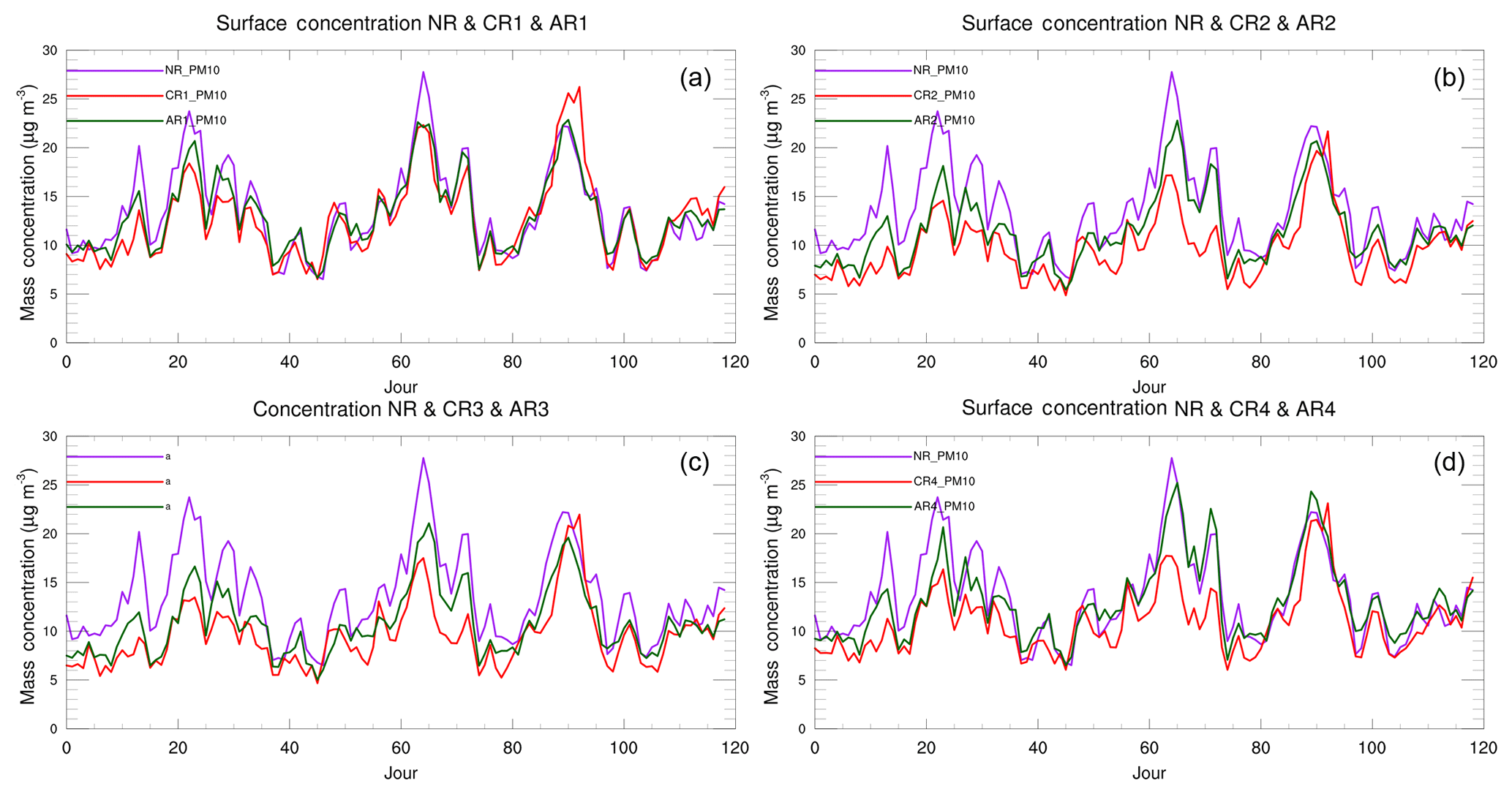
Figure 14 Median values over the AQeR station locations of the daily mean PM₁₀ surface concentration (µg m⁻³) for the NR (in purple) and the different CR (red) and AR (green) simulations (CR-AR-1 a, CR-AR-2 b, CR-AR-3 c and CR-AR-4 d).

Figure 15 Same legend as Fig. 14 for PM_2.5 concentrations.

To quantify the improvement in simulations through the assimilation of FCI synthetic observations during a severe-pollution episode for (7–15 March) over Europe, maps of relative concentrations of PM₁₀ and FGE are respectively represented for the CR comparison and for the AR comparison in Figs. 16 and 17. The simulations CR2, CR3 and CR4 underestimate PM₁₀ concentrations for 70 % over all Europe compared to the NR. The FGE presents high values from 0.55 to 0.85. The assimilation of synthetic AOD meaningfully improves the surface concentrations of aerosols over the continent in the simulations, but the simulations still underestimate the PM₁₀ concentrations by 30 %–20 %. Important changes in the FGE are noticeable, with values dropping from 0.55–0.85 down to 0.2–0.4 for all simulations. Over the other areas, the assimilation significantly reduces the relative bias and the FGE. Thus, the assimilation of synthetic observations significantly improves the representation of the surface PM₁₀ concentrations of simulations during the pollution episode.

Figure 16 PM₁₀ comparison between the NR and the CRs from 7 to 15 March 2014: relative bias and fractional gross error.

In summary, the use of synthetic observations at 444 nm of the future sensor FCI through assimilation significantly improves the aerosol fields of the simulations over the European domain from January to April 2014. These improvements are located all over the domain with best results over the European continent and the Mediterranean area. The improvement of the vertical profile of aerosol concentrations is also noticeable, and it may be explained because different parts of the column can be transported by winds in different directions (Sič et al., 2016), although the synthetic AOD observations do not provide information along the vertical. The first two simulations give better results over the ocean than simulations 3 and 4 due to a closer representation of the vertical profile of the aerosol concentrations. This may show an overly optimistic aspect of the OSSE of the first two simulations. The simulations lead to sufficiently reliable results since the shapes of their vertical profile of aerosol concentrations are different from those of the NR. These differences are caused by the way emissions are injected in the atmosphere (higher for simulation 3 and lower for simulation 4). The simulations 3 and 4 present robust results over the continent, despite the differences in the vertical representation of aerosol concentrations.

6 Discussion

Although the results have shown a general benefit of FCI/VIS04 future measurements for assimilation in the CTM MOCAGE, some limitations must be addressed. The AOD does not introduce information on the vertical distribution of PM, nor on the size distribution and type of aerosols. So, the performance of the assimilation will largely depend on the realism of the representation of aerosols in the CTM before assimilation. If, for instance, the model has a positive bias in AOD and a negative bias in surface PM₁₀ compared to observations, then the assimilation could lead to detrimental results. So the AOD and PM biases should be assessed and corrected as far as possible before assimilation in order to avoid detrimental assimilation.

To identify the added value of assimilating FCI/VIS04 AOD, the results need to be compared with the assimilation of present-day observations, such as imagers on LEO satellites and in situ surface PM observations. The assimilation of PM surface observations is indeed an efficient way to improve PM concentration fields at the surface (Tombette et al., 2009), but the correction of the fields remains confined to the lowermost levels. While improving the PM surface fields, it has been shown that the assimilation of AODs also gives a better representation of aerosols along the vertical (Figs. 12 and 13) and the AOD fields. Besides, the satellite coverage is much broader than the coverage of the in situ network and, for instance, aerosol fields over the seas can be corrected before they reach the coast.

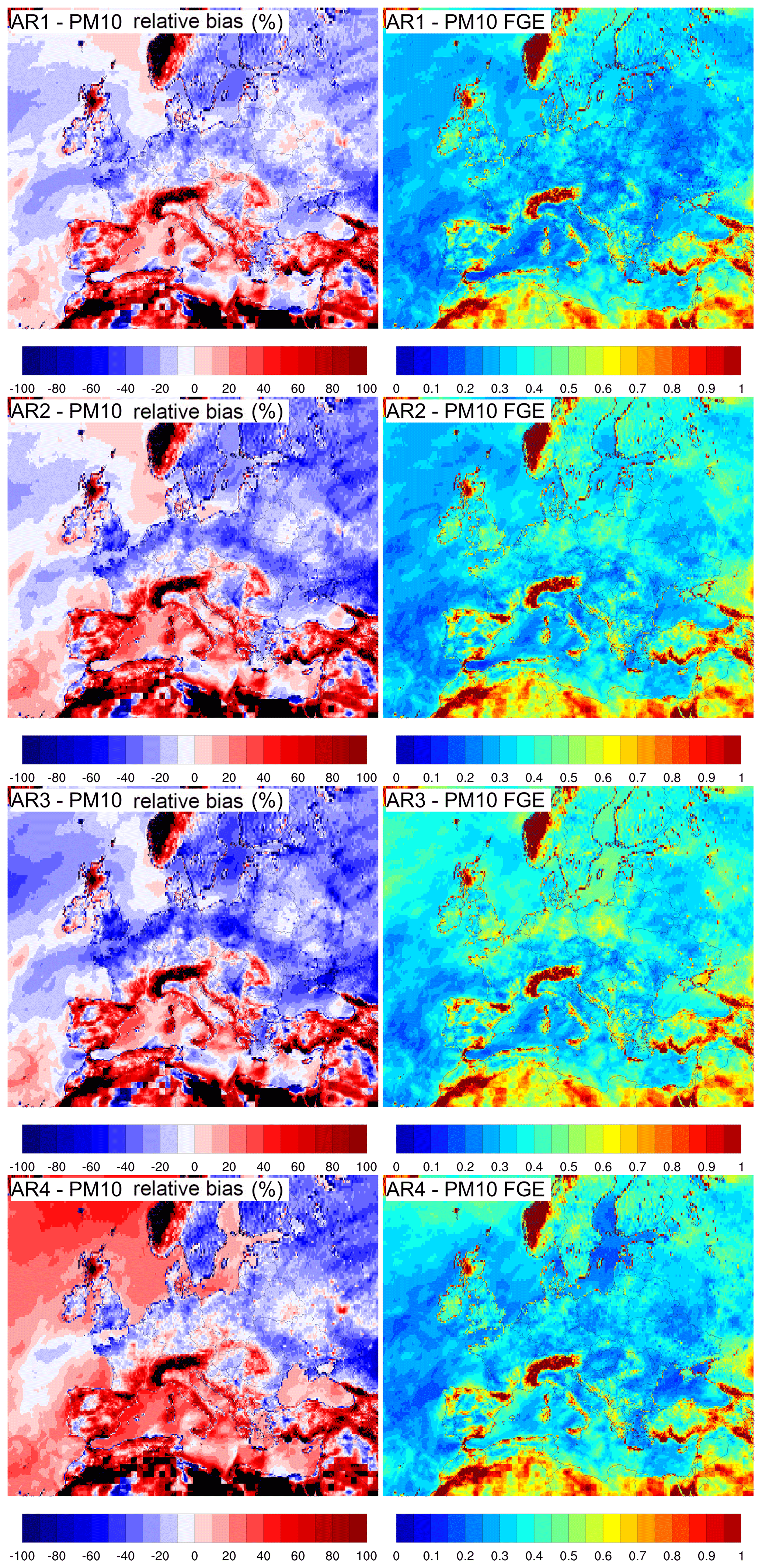
Figure 17 Same legend as Fig. 16, but for assimilation runs (AR) instead of control runs (CR).

Figure 18 Results of the assimilation run AR3LEO: density of assimilated synthetic observations (a ;to be compared with Fig. 6), time series of concentration of PM₁₀ at the surface for NR, CR3, AR3 and AR3LEO (b) between 1 January and 30 April 2014, PM₁₀ relative bias and FGE of AR3LEO from 7 to 14 March 2014 (to be compared with Fig. 17).

In order to assess the added-value of high-repetitivity measurements of FCI compared to a LEO satellite, a complementary experiment, called AR3LEO, has been done. This experiment is based on the CR3 configuration of MOCAGE, but the synthetic observations kept are only the ones at 12:00 UTC instead of the hourly observations. By taking into account only one measurement per pixel per day, AR3LEO should thus simulate the assimilation of a LEO satellite. The results of AR3LEO are in Table 9 and Fig. 18. The density of observations assimilated is about 10 times lower than the density of FCI assimilated data. Most of the scores (except the PM_2.5 correlation) of AR3LEO are between the CR3 and the AR3 scores, which shows and quantifies the benefit of FCI compared to a LEO satellite. This is also confirmed on the time series of PM₁₀ surface concentrations (Fig. 18): the AR3LEO simulation is closer to the CR3 simulation than to the AR3 simulation. During the pollution episodes from 7 to 14 March 2014 (Fig. 18, time series between day 60 and day 67, and maps), the amplitude of PM concentrations is underestimated more in AR3LEO than in AR3. The maps of bias and FGE show better scores in AR3 than in AR3LEO at the locations where pollution occurs.

The results have shown the potential benefit of assimilating AOD data from the future FCI/VIS04 in a chemistry transport model to monitor the PM concentrations on a regional scale over Europe. The horizontal and temporal resolutions of FCI (2 km horizontal grid every 10 min or even 2.5 min in Regional Rapid Scan) will, however, be much finer than the regional scales that have been considered in this study (0.2^∘ horizontal grid every hour). The large differences between the resolution of future FCI data and the data used in this OSSE have two important implications that deserve to be presented. Firstly, in order to get closer to the future data, one could consider generating synthetic observations at the full FCI resolution and assimilate them in a regional-scale assimilation system. The use of multiple observations using a “super-observation” approach, by spatial and temporal averaging, should reduce the instrumental errors and thus one may expect that the assimilation of real FCI data can lead to even better results than the OSSE presented here. Secondly, it is worth considering whether high-resolution FCI measurements could be assimilated in a high-resolution model for kilometre-scale monitoring of air quality. However, such work is presently limited by the present state of the art of numerical chemistry models and their input emission data. The conclusions of some recent numerical experiments with kilometre-scale air quality models (Colette et al., 2014) are that such models are very expensive and that the emission inventories do not have a sufficient resolution. Still, the performances of such high-resolution models are better than coarser resolution ones. As computing capacities keep increasing and kilometre-scale air quality models become affordable, it will be interesting to evaluate the benefit of assimilating high-resolution FCI data in a kilometre-scale air quality model, even if the emission data are built with coarse assumptions. One might expect that the assimilation of FCI data could correct the model state enough to balance the deficiencies of the emission inventories. For such a study, high temporal repetitivity may be also of great interest.

7 Conclusions

An OSSE method has been developed to quantify the added value of assimilating future MTG/FCI VIS04 AOD (444 nm) for regional-scale aerosol monitoring in Europe. The characteristic errors of the FCI have been computed from a sensitivity analysis and introduced in the computation of synthetic observations from the NR. An evaluation of the realistic state of the atmosphere of the NR has been done, as well as a comparison of CR simulations with the NR, in order to avoid the identical twin problem mentioned in Timmermans et al. (2009a). Furthermore, different control run simulations have been set up as in Claeyman et al. (2011) to avoid this issue. The results of the OSSE should hence be representative of the results that the assimilation of real retrieved AODs from the FCI sensor will bring.

Although the use of a single synthetic observation per profile and the choice of an albedo error of 10 % are pessimistic, the assimilation of synthetic AOD at 444 nm showed a positive impact, particularly for the European continental air pollution. The simulations with data assimilation reproduced spatial and temporal patterns of PM₁₀ concentrations at the surface better than without assimilation all along the simulations and especially during the high-pollution event of March. The improvement of analysed fields is also expected for other strong pollution event such as a volcanic ash plume. This capability of synthetic observations to improve the analysis of aerosols is present for the four sets of simulations which show the capability of future data from the FCI sensor to bring an added value into the CTM MOCAGE aerosol forecasts, and in general, into atmospheric composition models. Moreover, the advantage of a GEO platform over a LEO satellite has been shown and assessed.

The results over ocean show an increase in PM concentration bias after assimilation in some places, particularly for AR4. An explanation is that AOD does not introduce information vertically and that the correction of aerosols in the vertical relies on the model vertical distribution. For a satisfactory assimilation of AOD, the AOD and PM biases of the model should be assessed and corrected as far as possible. Another perspective is to use multiple wavelengths: using the Ångström exponent could avoid this problem by better distributing the increment of AOD between the different bins and hence the different species. Sič et al. (2016) also recommended the use of other types of observations, such as lidars, in the assimilation process to introduce information over the vertical.

The results presented here in this OSSE are encouraging for the use of future FCI AOD data within CTMs for the wavelength VIS04 centred at 444 nm. The use of other channels could bring complementary information, such as the NIR2.2, which is expected to be less sensitive to fine aerosols but more sensitive to large aerosols such as desert dust and sea salt aerosols. Future work may also consider exploiting the high-resolution of FCI, following two possible lines: either for regional-scale assimilation by using a super-observation procedure or for kilometre-scale air quality mapping and for assessing the quality of emission inventories. However, such an extension is mostly dependent on improvements in the numerical chemistry models, in the input emission data and in the optimization of assimilation algorithms.

Appendix A: Deriving AOD error variance from the global sensitivity analysis of FCI/VIS04 reflectance

The general method is summarized in Fig. A1. A sensitivity analysis was performed for each OPAC aerosol type, using Monte Carlo FCI simulations of about 200 000 draws in the prior distribution of the input parameters. The input distributions of AOD and total ozone and water vapour columns are obtained from a MOCAGE simulation that was run throughout the whole of 2013. The distribution of ground albedo is deduced from the OPAC database. The profiles of the MOCAGE simulation are classified into OPAC (Hess et al., 1998) types by matching species as in Ceamanos et al. (2014) and then applying classification criteria similar to the OPAC types.

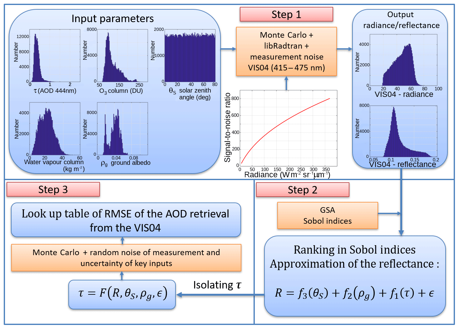
Figure A1 Summary of the methodology used to derive the RMSE of AOD from the FCI reflectance simulator. Step 1 is the computation of FCI radiance. Input parameters are the histograms of AOD, ozone total column, total water vapour content, ground albedo and solar zenith angle. The libRadtran simulator simulates the distribution of radiance and reflectance in the VIS04 channel and takes into account the signal-to-noise ratio of FCI. Step 2 is the approximation of the reflectance in functions of key parameters using a global sensitivity analysis method and Sobol indices. Step 3 is the retrieval of the AOD RMSE using random noise of measurement and the uncertainty of key parameters.

For every OPAC type, a global sensitivity analysis (GSA) was performed between the input (AOD τ, total column water vapour, ozone content), ground albedo ρ_g and solar zenith angle θ_S) distributions and the output (VIS04 reflectance) distributions of the FCI simulator. Under the assumption of independent inputs, the Sobol (1990, 1993) indices enable a ranking of inputs or couple of inputs with respect to their variance-based importance in the total output variance. For VIS04, the variability of the solar zenith angle, the ground albedo and the AOD are the three largest Sobol indices in that order and, together, they are at the origin of more than 98 % of the total variance of the output reflectance. Following Sobol (1996), the GSA can also be used to determine a truncated version of the Hoeffding (1948, ANOVA) functional decomposition with key inputs, which approximates the analysed reflectance. For all OPAC groups, the dependence of reflectance for VIS04 on the total ozone column and water vapour is negligible and is not taken into account in the reflectance approximation. As a consequence, the reflectance R can be approximated by the following equation:

$$\begin{array}{}\text{(A1)}& {\displaystyle }R=f_{\mathrm{3}}\left({\mathit{\theta }}_{\mathrm{S}}\right)+f_{\mathrm{2}}\left({\mathit{\rho }}_{\mathrm{g}}\right)+f_{\mathrm{1}}\left(\mathit{\tau }\right)+\mathit{ϵ},\end{array}$$

where f₁, f₂, and f₃ are functions of the solar zenith angle, the ground albedo and the AOD, respectively. The approximation error ϵ, exhibits a root mean square (rms) less than 0.7 W m⁻² sr⁻¹ µm⁻¹ (1.5 % of the mean radiance values of 47.3 W m⁻² sr⁻¹ µm⁻¹).

As a consequence of this sensitivity analysis, it is then possible to isolate the AOD τ with respect to the measured reflectance R, the other key inputs θ_S, ρ_g and the approximation error ϵ:

$$\begin{array}{}\text{(A2)}& {\displaystyle }\mathit{\tau }=F\left(R,{\mathit{\theta }}_S,{\mathit{\rho }}_{\mathrm{g}},\mathit{ϵ}\right).\end{array}$$

By sampling input distributions with this equation (Monte Carlo method), the RMSE of the AOD retrieval can be derived as a function of the reflectance R, the solar zenith angle θ_S, the ground albedo ρ_g and their uncertainties. R is associated with a measurement noise. No uncertainty is prescribed for the solar zenith angle. For a given fixed value of relative error of ground albedo, a look-up table is built that provides the RMSE of the AOD retrieval as a function of the solar zenith angle and the ground albedo. Such a look-up table of the RMSE of VIS04 AOD has been computed for every OPAC type and for different possible values of surface albedo errors.