Detecting cloud contamination in passive microwave satellite measurements over land

Remotely sensed brightness temperatures from passive observations in the microwave (MW) range are used to retrieve various geophysical parameters, e.g. near-surface temperature. Cloud contamination, although less of an issue at MW than at visible to infrared wavelengths, may adversely affect retrieval quality, particularly in the presence of strong cloud formation (convective towers) or precipitation. To limit errors associated with cloud contamination, we present an index derived from stand-alone MW brightness temperature observations, which measure the probability of residual cloud contamination. The method uses a statistical neural network model trained with the Global Precipitation Microwave Imager (GMI) observations and a cloud classification from Meteosat Second Generation-Spinning Enhanced Visible and Infrared Imager (MSG-SEVIRI). This index is available over land and ocean and is developed for multiple frequency ranges to be applicable to successive generations of MW imagers. The index confidence increases with the number of available frequencies and performs better over the ocean, as expected. In all cases, even for the more challenging radiometric signatures over land, the model reaches an accuracy of ≥70 % in detecting contaminated observations. Finally an application of this index is shown that eliminates grid cells unsuitable for land surface temperature estimation.

1 Introduction

Visible–infrared (vis–IR) satellite imagers provide excellent information about land surface characterization. Applications include land surface temperature estimations (e.g. Freitas et al., 2013), vegetation characteristics (e.g. Tucker et al., 2005), and surface water extent (e.g. Pekel et al., 2016).

These geophysical parameters can be retrieved accurately and with a good spatial and temporal resolutions from vis–IR observations, but only under clear-sky conditions. With clouds covering ∼60 % of the globe at any time (Rossow and Schiffer, 1999), there is a need for alternative sources of information. Passive microwave observations from satellites can partly fill this gap: they are much less sensitive to clouds and can provide valuable estimates of surface properties, despite their coarser spatial and temporal resolutions. Today, land surface temperature can be retrieved from IR observations for ∼60 % of the locations with a spatial resolution of 1 km² twice a day from polar orbiters (Prata et al., 1995) and with a spatial resolution of 2 km² every 15 min from geostationary satellites (e.g. Schmit et al., 2017). On the other hand, passive microwaves can provide this information with a spatial resolution of ∼20 km² twice a day over ∼100 % of the continents (Aires et al., 2001). Programmes are underway to merge these different observations for a complete spatial and temporal coverage. For instance, long time series of land surface temperature estimations with passive microwave observations are under construction, using different generations of passive microwave satellite instruments to be used in synergy with IR estimates (e.g. Prigent et al., 2016; Jiménez et al., 2017).

Although microwaves are less sensitive to clouds, the effect of clouds and rain on the microwave radiation increases with frequency. Multiple effects can occur, from liquid water clouds and rain emitting passive microwave radiation at the physical temperature of the cloud or rain to scattering by ice clouds that can lower the measured brightness temperatures, especially at high frequencies and for large ice contents. The cloud–rain effect that can be detected strongly depends on the surface type. The surface contribution to the passive microwave observations is proportional to the surface emissivity that changes from ∼0.5 over ocean to ∼1 over dry soil or dense forests. This means that the contrast between liquid particles in the cloud and rain and the surface will be usually larger over ocean than over land: cloud and rain liquid water emission increases the brightness temperature over the radiometrically cold ocean but will not show much contrast over the already radiometrically warm land. The opposite will prevail for frozen clouds, with the cloud scattering depressing the brightness temperature above the radiometrically warm land surface. Over ocean, passive microwaves have been extensively used to quantify the cloud liquid water and rain amounts (e.g. Greenwald et al., 1993; Kummerow et al., 1998). For ocean surface applications, cloud liquid water amount can usually be accounted for and the surface parameter estimation can compensate for the cloud impact, when atmospheric transmission is still high enough to have a significant contribution from the surface. Over land, cloud and rain detection using passive microwave is much more complicated (e.g. Spencer et al., 1989; Aires et al., 2001). First, surface emissivity is usually close to one, reducing the contrast between cloud and surface, and second, it changes spatially and temporally, e.g. with variations in soil moisture, vegetation density, or snow cover (e.g. Prigent et al., 2006). This can seriously affect the retrieval of land surface parameters when a cloud or rain effect is misinterpreted as a surface change.

The objective of this study is to develop a method that indicates a cloud–rain contamination on the passive microwave (MW) observations over land for different ranges of frequencies available on board the successive generations of passive MW satellite instruments. Rain detection schemes have been developed for the Special Sensor Microwave/Imager (SSM/I) over land: they are based on the scattering signal at 85 GHz and use decision trees (Grody, 1991; Ferraro, 1997). Cloud-filtering methods have also been derived for specific applications or for a given instrument. Long et al. (1999) analysed the brightness temperature time series at 85 GHz with different methods to remove the cloud perturbation on the SSM/I images for land surface applications. For the estimation of upper tropospheric humidity with satellite measurements around the water vapour line at 183.31 GHz, Buehler et al. (2007) developed filters with different channels around the line to avoid cloud-contaminated grid cells. Aires et al. (2011) used a neural network (NN) method trained on Meteosat Second Generation Spinning Enhanced Visible and Infrared Imager (SEVIRI) cloud products to create a cloud mask and a classification from the Advanced Microwave Sounding Units A and B (AMSU-A/AMSU-B) with channels from 23 to 183 GHz: statistical models were built separately over land and ocean to detect clouds or classify them into clear sky or low, medium, or high clouds.

Here, we use a similar approach to Aires et al. (2011) to develop a cloud–rain indicator over land for the passive MW imagers used for the estimation of land surface parameters over the last decades. Starting from the late 1970s with the Scanning Multichannel Microwave Radiometer (SMMR), a number of imagers have been launched over the years, including the Special Sensor Microwave Imagers (SSM/I, SSMIS), the Tropical Rainfall Measurement Mission (TRMM) Microwave Imager (TMI) (Kummerow et al., 1998), the Advanced Microwave Scanning Radiometers (AMSR-E, AMSR2), or the WindSat instrument (Gaiser et al., 2004). The latest instrument is the Global Precipitation Measurement (GPM) Microwave Imager (GMI) launched in 2014. Similar frequencies are used across the successive MW imagers, and they have relatively close characteristics (see Table 1) that could allow for similar processing of the data starting from 1978. We can divide the available instruments into three groups based on the imaging frequencies used on each of them:

• Below 40 GHz, a particular set of channels is available on board SMMR that flew from 1978 to 1987, as well as WindSat since 2003. The frequencies available on board GMI are 18.7 (V, H), 23.8 (V), and 36.5 GHz (V, H).

• Frequencies up to 90 GHz are available on the Special Sensor Microwave/Imager (SSM/I) (1987 to present), the Advanced Microwave Scanning Radiometer (AMSR-E/AMSR2) (2002 to present), and the Tropical Rainfall Measurement Mission (TRMM) Microwave Imager (TMI) between 1998 and 2015. On board GMI, the 89 GHz (V, H) frequency is added.

• Frequencies up to 190 GHz are, for instance, used for the Special Sensor Microwave Imager Sounder (SSMIS) (2003 to present) or GMI (2014 to present) with channels at 165.5 (V, H) and 183.3 GHz (V).

Table 1 Characteristics of the MW imagers over the years.

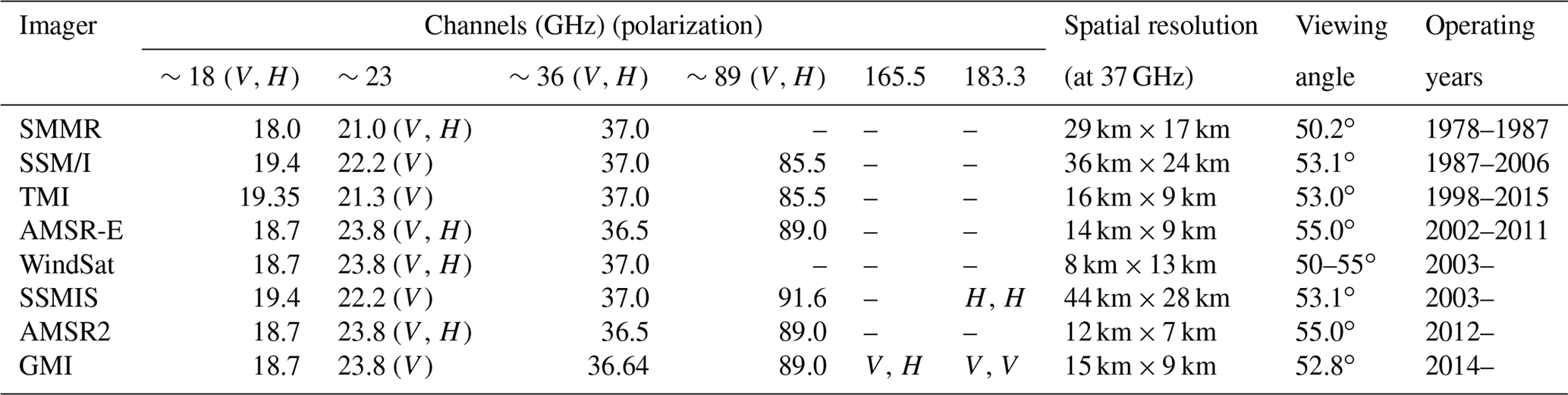
All these instruments observe with a similar incidence angle at the surface (as a consequence the angular dependence is not taken into account as with sounders such as AMSU). The available frequencies are close (e.g. 37 GHz for SSM/I against 36.5 GHz for GMI and AMSR2) and have small differences in the operating bandwidth. Note that frequencies below 18 GHz are available for some of these instruments, but they will not be considered here as their sensitivity to clouds is very limited. In this study, the passive microwave observations will come from GMI as it includes all the possible frequencies that we may want to use. Another benefit is that the GPM mission is not Sun synchronous and, as a result, it covers the full diurnal cycle, whereas the other instruments are Sun synchronous with overpassing times at the Equator in the morning and afternoon (SSMR, SSMI, and SSMIS) or at midday and midnight (AMSR-E and AMSR2). The cloud information comes from SEVIRI on board Meteosat: it provides a cloud mask as well as a cloud classification. Rain is not detected separately from the cloud per se: some clouds are likely to precipitate and the detection of these clouds will obviously include the detection of rain.

We first describe the data sets relevant for this study (Sect. 2). In Sect. 3, we will elaborate on the methodology. Results will be presented over land surfaces as well as over ocean (to illustrate the difference in behaviour over these two surface types), focusing on the detection of the cloud contamination on the MW observations over land (Sect. 4). Section 5 concludes this study.

2 Data sources

The different data sources are described here, namely the SEVIRI cloud classification and the GMI brightness temperatures (T_bs). The steps to create a consistent data set are described, along with a preliminary analysis of the observations. Using ancillary data to help characterize the atmospheric and surface conditions related to the cloud occurrence (such as land surface emissivity atlases) could help the cloud detection but at the cost of increasing the complexity to apply it. For flexibility and convenience, the detection of the cloud contamination will be exclusively built from passive MW observations.

2.1 Cloud mask and classification from Meteosat SEVIRI

Meteosat is a geostationary satellite positioned over the Equator. It covers mostly Africa, South America, Europe, and the Middle East, from ±60^∘ latitude and ±60^∘ longitude. The SEVIRI channels on board Meteosat encompass the visible and infrared ranges (Schmid, 2000), with varying pixel sizes around 3 km². Algorithms have been developed to provide cloud information, such as cloud-top height, water content, and also cloud classification, every 15 min over the whole field of view (Derrien and Le Gléau, 2005).

The Satellite Application Facility on Climate Monitoring (CMSAF) at the European Organisation for the Exploitation of Meteorological Satellites (EUMETSAT) has provided daily data since 2004. We used the 2013 version of the SEVIRI cloud classification algorithm, which provides a robust overview of the different cloud types that matter for vis–IR observations. Using this classification, the goal is to improve our understanding of the MW interaction with clouds and to detect the cloudy situations that impact the MW. Six full days each month in 2015 provide 72 different daily situations that represent a large variation in the possible cloud types and surface conditions, covering the full diurnal and annual cycles. The cloud classes are described in Table 2. High semi-transparent clouds are mostly cirrus of varying thickness, possibly over lower clouds. The fractional cloud class corresponds to cells that are only partly cloudy and to heterogeneous cloud cover. The other cloud types represent the continuum of possible cloud states, with varying opacity and height. Some of these clouds are likely to precipitate, and rain cases are naturally included in the database.

Table 2 Cloud classification from SEVIRI (Derrien and Le Gléau, 2005).

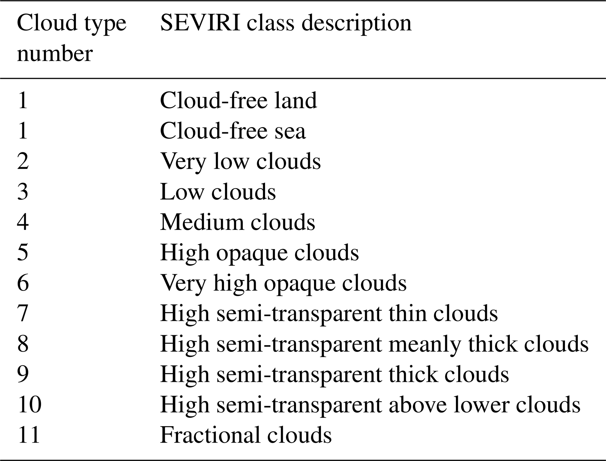
Figure 1 shows the latitudinal variation in the cloud types over land within the SEVIRI disk for February and August 2015. The intertropical convergence zone (ITCZ) location changes between the two seasons, as expected. Over the midlatitudes, the cloud frequency in February is higher than in August. The average relative frequency of each cloud type is displayed, showing that all cloud types are well represented.

Figure 1 Relative frequency of cloud types as a function of latitude for February (a) and August (b) 2015 over land within the SEVIRI disk. The average frequency of each cloud type over these 2 months is indicated in the legend.

2.2 The passive microwave observations from GMI

GPM relies on several instruments to provide a precipitation evaluation around the globe. The GMI is on board the core GPM satellite. The satellite has a 65^∘ inclination that allows a non-Sun-synchronous observation of the Earth. The available frequencies range from 10 to 183 GHz (Hou et al., 2014). In this study, we use the calibrated T_bs available in the level 1C-R product, where all the channels are projected to a common scan centre position, consistent with the 89 GHz channel resolution (4 km²).

GMI covers the full frequency range we want to analyse, with an incidence angle close to 53^∘. In this study, different subsets of the channels will be tested, corresponding to the different channel ranges available on the instruments since 1978. In addition, it observes at different local times, limiting possible biases related to observations at specific times of the day. The GMI data from 2015 have been downloaded for the 72 days corresponding to the SEVIRI selection.

2.3 Data set preparation and preliminary analysis

The SEVIRI and GMI data have very different spatial and temporal resolutions. We need to find the closest matching observations and relocate them on a common grid for further processing. Grid cells with a low-quality flag are avoided for both GMI and SEVIRI. Each GMI observation has a time stamp that is used to find the closest SEVIRI scan. With SEVIRI data every 15 min, there is a maximum of 7.5 min difference between GMI measurements and the corresponding SEVIRI classification. Given the spatial resolution, several SEVIRI cells will obviously fall in one GMI grid cell. In the training data set, only GMI observations associated with a unique target SEVIRI class are kept. There may be some mismatch between observed radiance and the SEVIRI cloud type due to inhomogeneous clouds at a scale lower than the footprint, especially for the lowest-frequency channels. This does not mean that GMI cells with heterogeneous cloud cover will not be able to be classified: it just limits the effect of ambiguous cases during the training phase.

The grid cells located above 55^∘ N and below 50^∘ S are discarded: they are larger in size in the SEVIRI data and are subject to more contamination by snow and ice. The GMI land mask is adopted to separate land and water bodies.

As a first analysis of the MW sensitivity to clouds, the distributions of the MW brightness temperatures (T_bs) are plotted in Fig. 2 for the different cloud types and for selected GMI frequencies over ocean (left) and land (right).

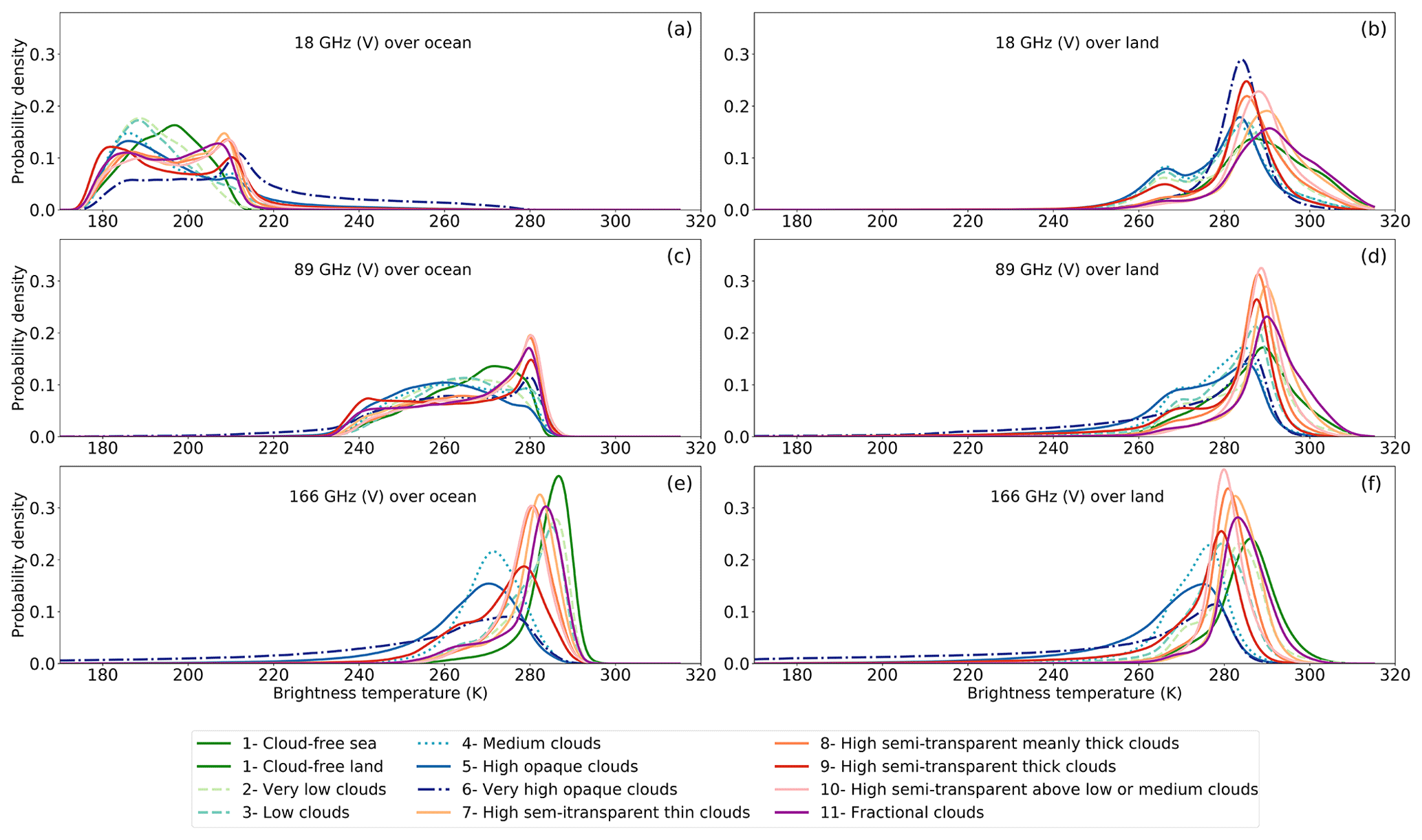
Figure 2 Probability distributions of the GMI-observed T_bs for various cloud types at 18 (a, b), 89 (c, d), and 166 GHz (e, f) for the vertical polarization over ocean (a, c, e) and land (b, d, f) from the filtered data set.

With increasing frequency, the atmospheric attenuation increases and the surface contribution to the signal decreases: the difference in the mean T_bs between the ocean and land situations diminishes with higher frequencies. Differences in the signal received by the instrument when it is not totally absorbed by the atmosphere can be due to the cloud effect but can also be related to changes in the surface properties (surface temperature of the ocean or land, wind speed at the ocean surface, soil moisture or vegetation density over land). Cloud types can be preferably associated with some environments, and the surface emissivity change with the surface conditions makes it difficult to find simple relationships between signals and cloud presence. In addition, water vapour modulates the MW signal, and this effect increases with frequency in the window channels.

Over ocean up to 100 GHz, the clouds are detectable and to some extent, their types can be distinguished: there is enough contrast between the radiometrically cold ocean background and the cloud radiation. Above 100 GHz, the surface contribution decreases drastically. The high opaque clouds can present low T_bs (the long left tail of the histogram) that are related to the scattering by the cloud-ice phase.

Over land at 18 GHz, the lowest peaks in the histograms for most cloud types (around 265 K) are likely related to the presence of water at the surface. Otherwise, at 18 GHz, the histograms are very similar for all land situations, meaning that this frequency has very limited sensitivity to the cloud presence and type. This can be seen as an asset for land surface characterization with these frequencies, as the signal will not be affected by the cloud presence. At high frequencies, the high opaque clouds present low T_bs (the left tails of the histograms) due to the ice scattering in the clouds (as at 166 GHz over ocean). These opaque clouds will likely be detected over land with these high frequencies.

3 Method

Our goal is to detect cloud contamination in the MW observations over land. It is not, at this stage, to classify cloud types. It will nevertheless be interesting to analyse the effects of each cloud type in the different frequency domains.

We focus here on the cloud detection for which a binary classification is required, but we will also experiment with the cloud-type classification. Several methods are available, some of which are rule-based, mostly by using thresholds for the various cloud types (e.g. the SEVIRI cloud algorithm by Derrien and Le Gléau, 2005, or the cloud filter at 183 GHz from Buehler et al., 2007). In this study, we use a statistical approach, similar to the one presented in Aires et al. (2011).

3.1 The training and testing data sets

The training and testing data sets are constructed using the collocated GMI observations and SEVIRI cloud information. To cover the full diversity of cloud situations, a full year of data have been sampled with 72 days (Sect. 2). The SEVIRI acquisition disk excludes the high-latitude regions and does not cover the full snow- and ice-free continents either. However, it was shown in Aires et al. (2011) that the calibration of a cloud classification on the SEVIRI disk with MW observations can be extrapolated to the other continents and we are confident that the methodology will be applicable outside the SEVIRI disk, excluding the snow and ice regions.

In the database, we ensure that every cloud type is equally represented. This process ensures that the obtained classification will not be biased towards the most frequent cloud situations, disregarding the less frequent ones. We therefore sample the same number of clear and cloudy situations, with each cloud type equally represented in the cloudy part. This resulted in 1 million samples for each of the 10 cloud types, and 10 million cloud-free samples. For a cloud classification model, with 11 different possible output classes, the database is built with a similar repartition of classes, giving around 11 million observations. The resulting databases are then randomly divided into the training (80 %) and the testing (20 %) data sets.

3.2 Statistical models

Several statistical models have been tested (e.g. tree-based or logistic regression, results not shown) but we kept an NN classification, based on the MultiLayer Perceptron (MLP) (Rumelhart et al., 1986b). MLPs are universal non-linear approximators, that can, given enough parameters, approximate any function (Hornik, 1991). The NN inputs are the MW channels, their number depending on the frequency ranges (5, 7, or 11). Five neurons (7 and 9) in the hidden layer are used. More neurons and a larger network have been tested, but they did not offer significant improvements in the resulting accuracy (results not shown). The output layer is composed of one binary output (for the cloud detection) or 11 binary outputs (for the cloud classification). The activation in the output layer is a softmax function. The parameters of the MLP classifier are found during the learning stage, in which a binary cross-entropy loss function (Dreiseitl and Ohno-Machado, 2002) is minimized with the back-propagation algorithm (Rumelhart et al., 1986a). Using this loss function allows the continuous output of the NN to be interpreted as a classification probability (Bridle, 1989). The models are implemented using the Keras library (Chollet et al., 2015), and the training is stopped when the loss is not decreasing for five consecutive epochs, which happens after a few hundred epochs depending on the network and input size. The hardware used for this step is a standard office laptop, with four cores and 16 Gb of RAM. After training, the prediction closest to 0 indicates a high probability of having a cloudy grid cell (1 for clear sky). The result of the continuous NN output can then be converted into a binary decision using a threshold to be defined. In the following graphs and results, if not otherwise specified, a decision threshold of 0.5 is applied to derive the binary classification. For multi-class outputs, the highest value among the output neurons is selected as the predicted class. The results are displayed showing the percentage of true positives (cloudy grid cells correctly detected), and true negatives (clear grid cells correctly predicted) from all the samples inside a test set.

4 Results

We first test the methodology over ocean, where clouds are expected to be easier to detect and quantify as we saw from the distributions in Fig. 2. It provides a testing ground for the method, before expanding it to the more difficult land case.

4.1 Detecting clouds over ocean

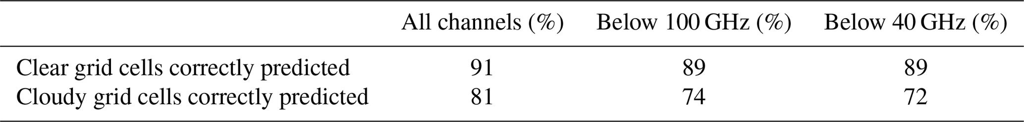
As described in Sect. 3.1, the database is created with an equal distribution of cloudy and clear conditions and a balanced repartition between the different cloud types. The cloud detection is evaluated for the three MW frequency ranges (all channels, below 100 GHz only, below 40 GHz only), and the results are presented in Table 3 for the test data set. The cloud detection performs well over ocean, reaching at least 80 % accuracy, even with a reduced number of channels. The low emissivity of the ocean (∼0.5) and its relative homogeneity makes it possible to correctly detect the cloud presence, even at low MW frequencies.

Table 3 Results of a binary classification over the ocean for different MW frequency ranges.

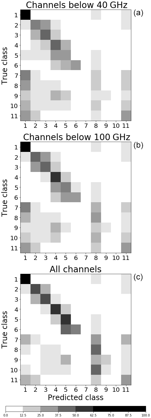
These cloud detection results are very encouraging and the natural next step is to investigate a cloud classification over ocean, with the same MW frequency ranges. The data set is used with all classes equally sampled, making it suitable for a multiclass classification. Similar NN schemes are implemented, with 11 possible output neurons representing the 10 cloud classes and the clear case for the three frequency ranges. The confusion matrices (Fig. 3) display the results of the classification, showing for each class (y axis) the percentage of samples predicted to belong to 1 of the 11 possible SEVIRI classes (x axis). The diagonal of the confusion matrix shows the correctly classified percentage for each cloud type. The highest accuracy is reached for the cloud-free ocean for the three MW frequency ranges. It is occasionally confused with the high semi-transparent meanly thick clouds (class 8) or the fractional clouds (class 11) as they may not significantly affect the measured T_bs. For opaque clouds (classes 2–6), the highest percentages are near the diagonal: these cloud types are correctly classified or classified as a cloud with a similar altitude. We see an increase in the detection of high opaque clouds (classes 4, 5) when the channel at 89 GHz is available. This can be explained by the increased detection of the ice content that this channels offers compared to lower frequencies. When all channels are available the discrimination between cloud layers is even easier, resulting in a better classification. The high semi-transparent clouds (classes 7, 8, 9, and 10) are sometimes incorrectly classified as clear sky, especially with only lower frequencies (due to channels less sensitive to high-altitude phenomena), or high semi-transparent thick clouds (class 8) with higher frequencies, which is expected given that they share similar properties (such as cloud height). Fractional clouds (class 11) are not well classified, the predicted class being either cloud-free or high semi-transparent (class 8).

Figure 3 Confusion matrix over the ocean for the cloud type classification for the three MW frequency ranges: below 40 GHz (a), below 100 GHz (b), and all channels (c). The cloud type numbers are detailed in Table 2.

4.2 Detecting clouds over land

A similar cloud detection method is applied over land. The NN classifiers are built using the three different MW frequency ranges as inputs and with one output indicating the clear vs. cloudy probability.

The specifics of the model and database are described in Sect. 3.1 and 3.2. Similar to Table 3 over ocean, Table 4 (top part) presents the accuracies reached over land by the three frequency ranges. The classification performance deteriorates compared to the ocean case, as expected. Nevertheless, even for the worst case (with only five low frequency channels available), true positive and negative detections are close to 70 %.

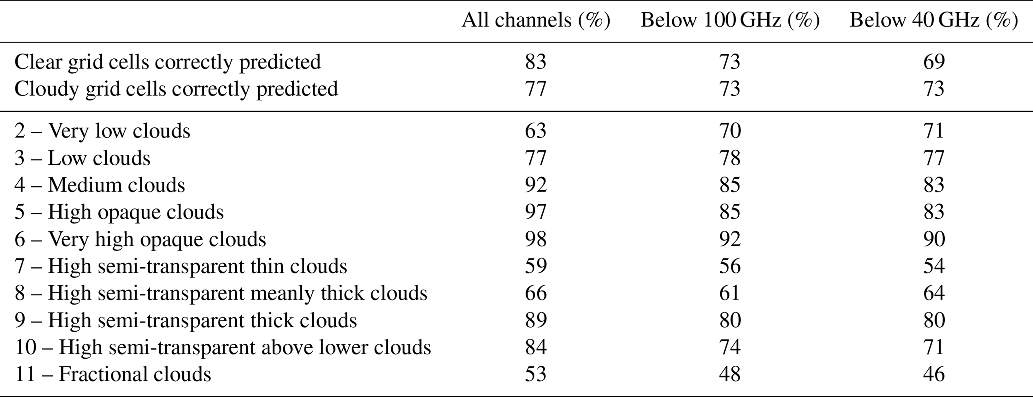
The result of the detection has been analysed further, as a function of the cloud type (lower part of Table 4). Note that these are only a detail of the previous results (top part of Table 4) separated by each original cloud type. Large differences are observed between cloud types. For non-semi-transparent clouds, the higher the cloud the better the detection rate: this is directly related to the presence of ice in high clouds that can scatter the MWs. The higher the frequency, the better the detection of ice phase. Likewise, high semi-transparent clouds can be detected only when they are thick enough.

Table 4 Top part shows percentage of correct cloud detection from the test set over land. Lower part shows details of the percentage of each cloud type predicted as cloudy. The results are presented for the three MW frequency ranges.

4.3 Detecting cloud-contaminated microwave observations over land

The previous results showed that MWs cannot detect all clouds seen by vis–IR measurements, especially when only a subset of the frequencies is available. This behaviour is actually very attractive for “all weather” land surface applications with MWs. However, for accurate land surface characterization with MW, we need to identify the cloudy situations that really contaminate the MW. To that end we use the results from the previous model to select an appropriate definition of cloud contamination in the MW. For all frequency ranges, high semi-transparent thin clouds, high semi-transparent meanly thick clouds, and the fractional clouds (i.e. classes 7, 8, and 11), the classification accuracy is close to 50 %, similar to a random class assignment, meaning that these frequency ranges are not affected enough by these cloud types to be able to detect them. To focus on the clouds that do impact the MWs, we rebuild a training data set, suppressing the three ambiguous classes previously mentioned (namely classes 7, 8, and 11). The idea behind this new training database is that removing ambiguities at the learning stage will improve the classification. In other words, removing the ambiguous SEVIRI cloud types from the training database allows the model to ignore these phenomena, which are mostly detected in vis–IR. The lower sensitivity to clouds in MW is thus accounted for in the new training data set.

The results of this new classification are provided in Table 5, separately for the clear grid cells (class 1), for the cloudy grid cells with clouds that do contaminate the MW (the MW cloud-contaminated grid cells, i.e. classes 2, 3, 4, 5, 6, 9, and 10), and for the cloudy grid cells corresponding to the three cloud types that are difficult to detect with MW (the ambiguous grid cells, ignored in the training data set, i.e. classes 7, 8, and 11).

Table 5 Classification results for the different clear and cloudy populations for the three MW frequency ranges. See text for more details.

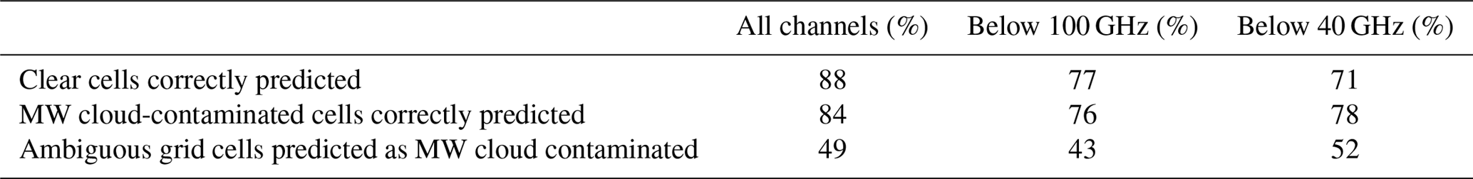
The results show that the clear-sky detection increases and so does the detection of MW cloud-contaminated cells (84 % with all frequencies) compared to the detection of cloudy cells in Table 4 (77 % with all frequencies). This is expected, as the ambiguous cases have been removed from the statistics; it is also consistent with the number of ambiguous cells (ignored in the training data sets) that are predicted as MW cloud contaminated by the new classification (close to 50 % regardless of the frequency range).

The original output of the classification is not binary, but a number between 0 and 1 (see Sect. 3.2). In the results shown so far a decision threshold at 0.5 has been adopted to separate the two classes. Would it be possible to adjust this threshold for a better detection of the cloud-contaminated observations? Figure 4 presents the outputs of the NN classifier for the three populations previously defined in Table 5 and for each MW frequency range (Fig. 4).

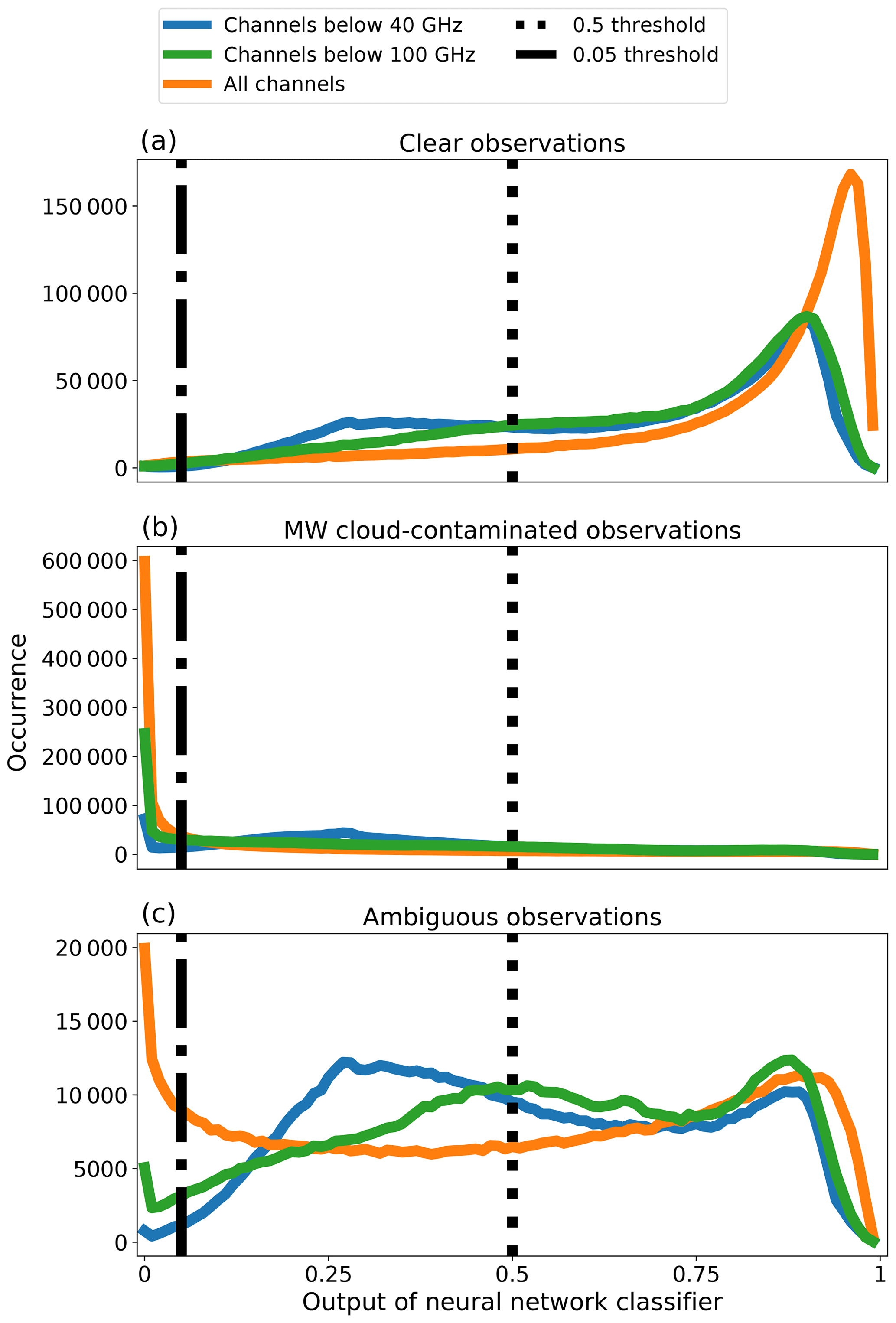
Figure 4 Model output probability distributions for the clear grid cells (a), the MW cloud-contaminated grid cells (b), and for the ambiguous grid cells (c), for the three MW frequency ranges. See text for more detail about the three populations.

Figure 4 (top and middle panels) confirms that the clear grid cells and the MW cloud-contaminated grid cells are confidently classified, with very distinct output distributions for these two populations, 0 indicating a high confidence to be in the MW cloud-contaminated class and 1 a high confidence to be in the clear class. Nevertheless, when channels above 100 GHz are not available, a non-negligible fraction of the clear grid-cell population is classified between 0.1 and 0.4, meaning that the confidence in the prediction is lower. For the ambiguous cloud types that were ignored during the training (bottom panel), the distribution of the outputs covers a large range of values, conveying the uncertainty in the prediction. However, with the full frequency range there are a number of observations labelled as confidently contaminated (peak in low NN output values); this can be expected due to the better sensitivity of the high-frequency channels to thin clouds. Figure 4 clearly shows that, depending on the decision threshold selected for the NN output values, it is possible to filter out more or less ambiguous grid cells. So far it has been at 0.5, but it could be modified. The selection of this threshold should depend on the frequency range and the application.

For instance, for land surface temperature estimates, the idea is to avoid the clouds that really affect the low microwave T_bs (below 40 GHz) that are used for the retrieval of this parameter (e.g. Prigent et al., 2016; Jiménez et al., 2017). Note, however, that this does not exclude the use of the higher frequencies for cloud-contamination detection if these frequencies are also available. In addition, the interest of the MW for the land surface temperature estimation is to complement the infrared estimations that are not available under cloudy conditions: as a consequence, only the seriously cloud-contaminated MW observations should be detected to maintain a quasi “all weather” coverage of the MW estimates while limiting erroneous estimates under very cloudy/rainy situations. In that framework, the role of the cloud classification is to make sure the cloud-contaminated observations are correctly detected. The correct detection of the true clear cases is of lesser importance.

Figure 5 presents the percentage of MW observations predicted as cloud contaminated, as a function of the threshold on the NN classifier output for both the MW cloud-contaminated cases (the true positive, solid line) and the clear-sky cases (the false positive, dashed line). It shows that a threshold below 0.1 keeps the percentage of misclassified clear-sky cases low (low percentage of false positives). Combined with the results from Fig. 4 (middle panel), a threshold at 0.05 and 0.01 could also be tested to only classify the cloud-contaminated observations with a high degree of confidence.

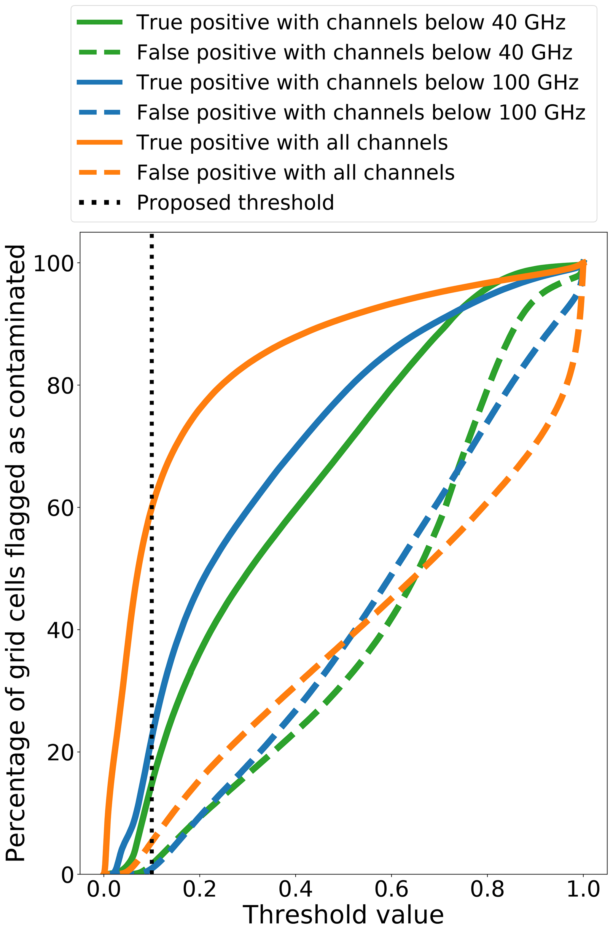
Figure 5 Evolution of the percentage of MW observations correctly classified as cloud contaminated (true positive, solid lines), and clear-sky grid cells incorrectly classified as being contaminated (false positive, dashed line), as a function of the NN output threshold for the three MW frequency ranges. Note that, for this data set, half the observations are cloudy according to SEVIRI.

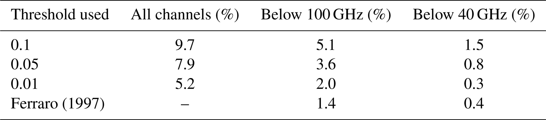
A day of GMI observations, 15 June 2015, is selected to illustrate the potential of the classification of the MW cloud contamination. Note that this day is not included in the training or testing data sets previously used. For the three MW frequency ranges, the classification is applied with the selected thresholds (0.1, 0.05, 0.01). Table 6 provides the percentage of observations classified as cloud contaminated for each set-up, along with the results from the Ferraro (1997) precipitation detection algorithms based on a decision tree and thresholds on channels. As expected, when the high-frequency channels are included, the sensitivity of our methodology to the cloud contamination increases, as does the percentage of cloud-contaminated observations, with ∼10 % cloud-contaminated observations for this frequency range. Note that, for that day, the coincident SEVIRI observations are cloudy at 29 %, i.e. 3 times more than the results from the highest detection of the high MW frequency range. Using only frequencies below 40 GHz, the percentage of cloud-contaminated observations decreases. This illustrates the benefit of using lower MW frequency channels for “all weather” land surface characterization, with a ratio of 4 between the number of contaminated observations when adding the 89 GHz to the frequencies below 40 GHz (using the 0.05 threshold). For all these threshold–model combination, the number of clear-sky observations (according to SEVIRI) incorrectly flagged stays below 0.5 % of all observations.

For comparison purposes, the Ferraro (1997) rain detection algorithms are also run and compared to both the algorithm using the 85 GHz channel and the one limited to the frequencies below 40 GHz. The results in the last line of the table show the number of observations that are flagged as precipitating. As expected the number of precipitating situations is lower than the number of cloud-contaminated MW observations. For the models with channels above 40 GHz, more than 90 % of the precipitating observations are detected by our method. The model with only channels below 40 GHz still retrieves more than 50 % of the precipitating observations when the 0.1 threshold is used.

Nevertheless, depending on the applications and the degree of uncertainty required in the land surface product, if the full frequency range up to 100 GHz is available on the instrument, it can be relevant to use all the frequencies up to 100 GHz to filter out the cloud-contaminated grid cells, even if only the frequencies below 40 GHz are used in the retrieval of the land surface parameter. As an example, if the land surface temperature is to be retrieved with very low uncertainty from SSM/I observations (an instrument that has channels up to 90 GHz), it can be wise to use the full frequency range to detect the cloud contamination, even if only the lower frequencies below 40 GHz are used in the retrieval.

Ferraro (1997)

Table 6 Percentage of MW observations classified as cloud contaminated for the three MW frequencies ranges, with different thresholds on the NN classifier output. Results are presented for 15 June 2015 over land surfaces within the SEVIRI disk. The last line of the table presents the percentage of observations detected as precipitating with the Ferraro method using channels up to 100 GHz or only below 40 GHz.

Now that we have an estimate of the number of points that are flagged by each model with different thresholds we can plot the global map of the locations of these contaminated cells. Figure 6 shows the results for the three different frequency groups and with three thresholds applied. The thresholds were chosen based on the results in Table 6 to illustrate how different thresholds might be applied to each model while still providing coherent estimates of cloud-contaminated grid cells.

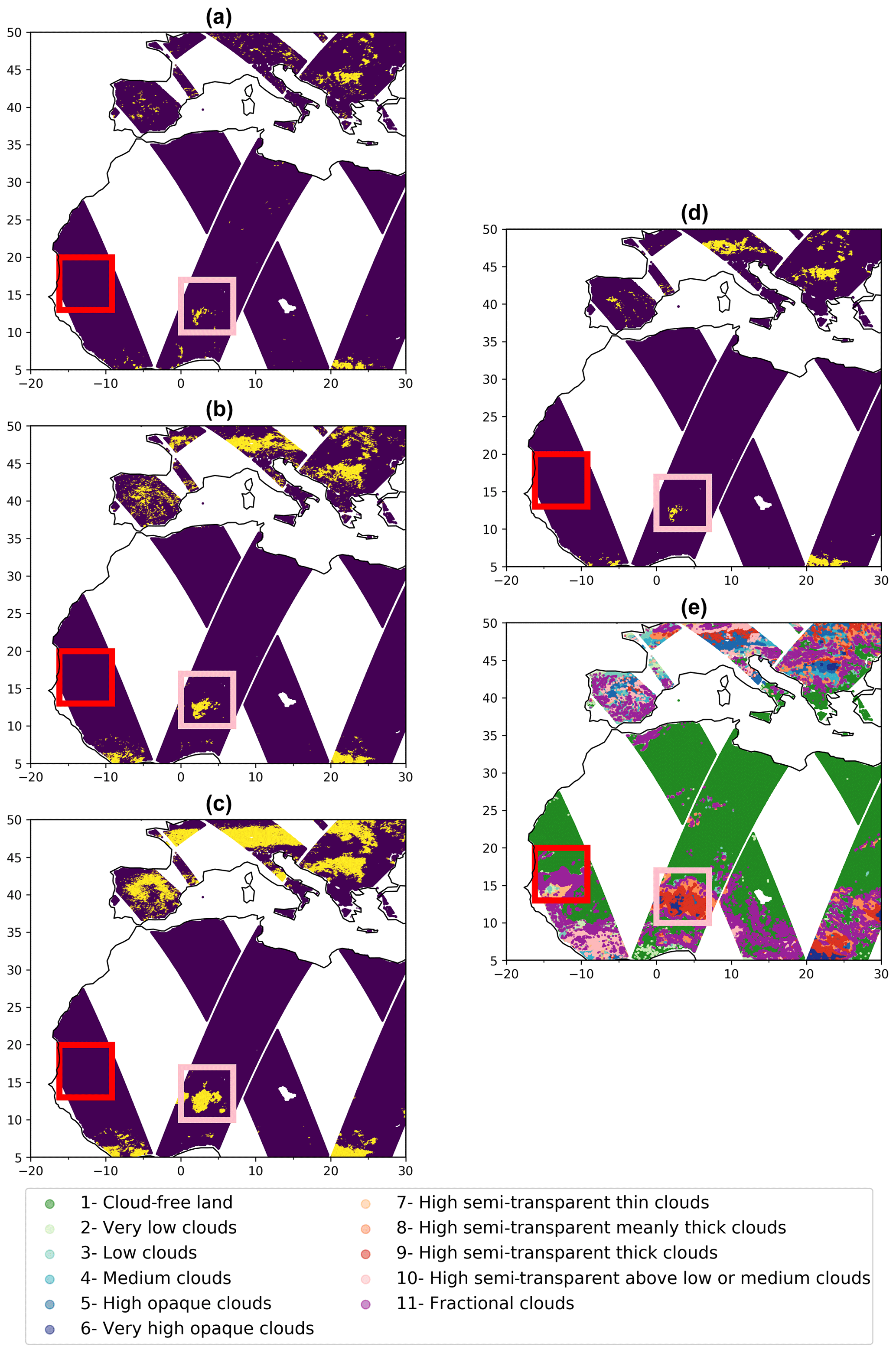
Figure 6 Maps showing for the 15 June 2015: (a) the predicted grid cells flagged by the model using channels below 40 GHz with a 0.1 threshold; (b) by the model using channels below 100 GHz with a 0.05 threshold; (c) by the model using channels below 190 GHz with a 0.01 threshold; (d) the detected precipitating cells according to Ferraro (1997); and (e) the cloudy classes from SEVIRI. The red and the pink square boxes highlight two smaller regions further discussed in Sect. 4.3.

In Fig. 6, models are applied to the data over land to create the three maps. For each map a different threshold is applied: 0.1 with the lowest channels (a), 0.05 with channels up to 100 GHz (b) and 0.01 with all channels available (c). The fourth subplot (d) is the precipitating observations according to Ferraro's 89 GHz algorithm. The fifth subplot (e) shows the SEVIRI cloud type. We can analyse the output of this map:

• The agreement between models and the increased number of flagged points with more channels is clearly visible (a, b, c).

• In some areas, the cloudy grid cells do not appear to be detected (i.e. red area). When looking at the detail of the SEVIRI cloud types (subplot e) in that area we find out they are mostly fractional/semi-transparent or low clouds, which explains the low contamination rate, according to our definition.

• In the pink area, we have a stronger detection of contaminated grid cells. Indeed the most represented cloud types are high semi-transparent thick clouds (23 %), high semi-transparent clouds above low or medium clouds (20 %), and very high opaque clouds (17 %). All these cloud types are the ones that might affect the measurement the most.

• We find that the precipitating observations are correctly found within the detected cloudy cells, but there are more cloud-contaminated observations.

This global application of our models shows the possible use of different frequency ranges to detect contaminated observations. Although adding more information by using the channels more sensitive to ice content leads to a better detection of cloud contamination, we show here that it is possible to filter out cloud-contaminated measurements even above land with a restricted number of channels. The thresholds used here are coherent for the specific application shown in this study, with a low number of misclassified clear-sky grid cells and also with the real-world occurrence of deep convective phenomena that contaminate the observations the most. Indeed, the International Satellite Cloud Climatology Project (ISCCP) data show that they have an average occurrence of 2.6 % for deep convections that is of the same magnitude as our cloud index associated with the proposed thresholds (Rossow and Schiffer, 1999).

5 Conclusions

Passive microwave observations from satellites are less sensitive to clouds than visible–infrared measurements and can provide an almost “all weather” land surface characterization. However, cloud (and possible rain) can affect the microwave observations, even at frequencies below 40 GHz. For an accurate estimation of land surface parameters, cloud-contaminated MW observations have to be detected to avoid interpreting a cloud presence as a surface change.

A methodology has been developed to detect cloud contamination on passive MW observations over land (except snow- and ice-covered areas). It is based on a NN classification, trained on collocated SEVIRI cloud types. The NN output indicates the probability of cloud contamination in the MW signal for a given MW frequency range. The cloud-contamination index is provided with values in the 0–1 range: the threshold applied to this index can be customized to fit the required application needed to flag out the contaminated observations. Although the target here is cloud detection over land surfaces, the model was also tested over the simpler case of detection over ocean. The index confidence increased with the number of channels available and performed better over the ocean as expected. In all cases, even with a reduced number of information over land, the detection of contaminated observations is performed with more than 70 % accuracy.

An example of a possible application of this cloud-contamination index was shown to eliminate grid cells unsuitable for land surface temperature estimation. The index proved useful to signal cloud contamination for this particular application and will soon be applied to the quality control of a long time record of land surface temperatures (Prigent et al., 2016). The land surface temperature estimate is essentially based on passive microwave frequencies between 18 and 40 GHz, from a succession of satellite imagers since 1978 (SMMR, SSM/I, and SSMIS). The first instrument only measured up to 36 GHz, contrarily to the last instruments. So far, the cloud and/or rain detection indices are based on thresholds related to channels around 85 GHz (Jiménez et al., 2017). This frequency is not available on board SMMR and the new methodology for the frequency range below 40 GHz will be applied to the full data set, with possible comparisons with the current method up to 100 GHz, when these channels are available. Overall the models developed in this study can be applied globally in ice- and snow-free areas and are potentially useful for numerous applications where it is of interest to identify possible cloud contaminations in observed MW radiances. In addition to the land surface temperature example, this index can be useful for selecting clear scenes for accurate MW emissivity estimation (Moncet et al., 2011) or to detect cloudy scenes for the analysis of deep convections (Prigent et al., 2011).