the Creative Commons Attribution 4.0 License.
the Creative Commons Attribution 4.0 License.
 | 09 May 2019
Characterization of a commercial lower-cost medium-precision non-dispersive infrared sensor for atmospheric CO2 monitoring in urban areas
Emmanuel Arzoumanian
Ana Bastos
Bakhram Gaynullin
Olivier Laurent
Michel Ramonet
Philippe Ciais
CO2 emission estimates from urban areas can be obtained with a network of in situ instruments measuring atmospheric CO2 combined with high-resolution (inverse) transport modelling. Because the distribution of CO2 emissions is highly heterogeneous in space and variable in time in urban areas, gradients of atmospheric CO2 (here, dry air mole fractions) need to be measured by numerous instruments placed at multiple locations around and possibly within these urban areas. This calls for the development of lower-cost medium-precision sensors to allow a deployment at required densities. Medium precision is here set to be a random error (uncertainty) on hourly measurements of ±1 ppm or less, a precision requirement based on previous studies of network design in urban areas. Here we present tests of newly developed non-dispersive infrared (NDIR) sensors manufactured by Senseair AB performed in the laboratory and at actual field stations, the latter for CO2 dry air mole fractions in the Paris area. The lower-cost medium-precision sensors are shown to be sensitive to atmospheric pressure and temperature conditions. The sensors respond linearly to CO2 when measuring calibration tanks, but the regression slope between measured and assigned CO2 differs between individual sensors and changes with time. In addition to pressure and temperature variations, humidity impacts the measurement of CO2, with all of these factors resulting in systematic errors. In the field, an empirical calibration strategy is proposed based on parallel measurements with the lower-cost medium-precision sensors and a high-precision instrument cavity ring-down instrument for 6 months. The empirical calibration method consists of using a multivariable regression approach, based on predictors of air temperature, pressure and humidity. This error model shows good performances to explain the observed drifts of the lower-cost medium-precision sensors on timescales of up to 1–2 months when trained against 1–2 weeks of high-precision instrument time series. Residual errors are contained within the ±1 ppm target, showing the feasibility of using networks of HPP3 instruments for urban CO2 networks. Provided that they could be regularly calibrated against one anchor reference high-precision instrument these sensors could thus collect the CO2 (dry air) mole fraction data required as for top-down CO2 flux estimates.
- Article
(1462 KB) - Full-text XML
-
Supplement
(560 KB) - BibTeX
- EndNote


The works published in this journal are distributed under
the Creative Commons Attribution 4.0 License. This license does not affect
the Crown copyright work, which is re-usable under the Open Government
Licence (OGL). The Creative Commons Attribution 4.0 License and the OGL are
interoperable and do not conflict with, reduce or limit each other.
© Crown copyright 2019
Urban areas cover only a small portion (< 3 %) of the land surface but account for about 70 % of fossil fuel CO2 emissions (Liu et al., 2014; Seto et al., 2014). Uncertainties of fossil fuel CO2 emissions from inventories based on statistics of fuel amounts and/or energy consumption are on the order of 5 % for OECD countries and up to 20 % in other countries (Andres et al., 2014) but they are larger in the case of cities (Bréon et al., 2015; Wu et al., 2016). Further, in many cities of the world, there are no emission inventories available. The need for more reliable information on emissions and emission trends has prompted research projects seeking to provide estimates of greenhouse gas (GHG) budget cities, power plants and industrial sites. These are often based on in situ measurements made at surface stations (Staufer et al., 2016; Lauvaux et al., 2016; Verhulst et al., 2017), aircraft campaigns around emitting locations (Mays et al., 2009; Cambaliza et al., 2014) and satellite imagery (Broquet et al., 2018; Nassar et al., 2017). Although sampling strategies and measurement accuracies differ between these approaches, the commonly used principle is to measure atmospheric CO2 dry air mole fraction gradients at stations between the upwind and downwind vicinity of an emitting area and infer the emissions that are consistent with those CO2 gradients and their uncertainties, using an atmospheric transport model. This approach is known as atmospheric CO2 inversion or as a “top-down” estimate.
Inversion studies from Paris, France, attempting to constrain CO2 emissions from measurements of CO2 dry air mole fractions at stations located around the city along the dominant wind direction have pointed out that the fast mixing by the atmosphere and the complex structure of urban CO2 emissions require high-resolution atmospheric transport models and continuous measurements of the atmosphere to select gradients induced by emission plumes (Breton et al., 2015; Wu et al., 2016) that can be captured at the scale of the model.
With the existing three stations, the CO2 emissions from the Paris megacity could be retrieved with an accuracy of ≈20 % on monthly budgets (Staufer et al., 2016). A denser network of stations would help to obtain more information on the spatial details of CO2 emissions. A network design study by Wu et al. (2016) for the retrieval of CO2 emissions per sector for the Paris megacity has shown that with 10 stations measuring CO2 with 1 ppm accuracy on hourly time steps, the error of the annual emission budget could be reduced down to a 10 % uncertainty. Wu et al. (2016) furthermore found that for a more detailed separation of emissions into different sectors, more stations were needed, on the order of 70 stations to be able to separate road transport from residential CO2 emissions. This inversion based on pseudo-data allowed the estimation of total CO2 emissions with an accuracy better than 10 % and emissions of most major source sectors (building, road energy) with an accuracy better than 20 %. Another urban network design study over the San Francisco Bay Area reached a similar conclusion, i.e. that in situ CO2 measurements from 34 stations with 1 ppm accuracy at an hourly resolution could estimate weekly CO2 emissions from the city area with less than 5 % error (Turner et al., 2016).
In the studies from Wu et al. (2016) and Turner et al. (2016), the additional number of atmospheric CO2 measurement stations rather than the individual accuracy of each measurement helped to constrain emissions, provided that CO2 observation errors have random errors of less than 1 ppm on hourly measurements, uncorrelated in time and in space between stations. Therefore, we will adopt here a 1 ppm uncertainty on hourly CO2 data as the target performance for new urban lower-cost medium-precision CO2 sensors.
Today, the continuous CO2 gas analyzers used for continental-scale observing systems like ICOS (https://www.icos-ri.eu/, last access: 30 April 2019), NOAA (https://www.esrl.noaa.gov/gmd/, last access: 30 April 2019) or ECCC's GHG network (https://www.canada.ca/en/environment-climate-change.html, last access: 30 April 2019) follow the WMO GAW guidelines and are at least 10 times more precise than our target of 1 ppm, but are also quite expensive. For urban inversion-based flux estimates for Paris, Wu et al. (2016) found that the number of instruments is more important than their individual precision. Furthermore, Turner et al. (2016) reported that weekly urban CO2 fluxes in the San Francisco Bay Area (California, USA) can be estimated at a precision of 5 % when deploying a dense network of sensors (ca. every 2 km) with an assumed mismatch error of 1 ppm. This underlines that significant expansion of urban networks is desirable and could be achieved at an acceptable cost if low-cost sensors could be produced with the specifications of 1 ppm random error (i.e. bias-free long-term repeatability).
Recently, inexpensive sensors, measuring trace gases, particulate matter and traditional meteorological variables, using various technologies and accuracy have become commercially available. Evaluation and implementation of these sensors is quite promising (Eugster and Kling, 2012; Holstius et al., 2014; Piedrahita et al., 2014; Young et al., 2014; Wang et al., 2015). With the advent of low-cost mid-IR light sources and detectors, different non-dispersive infrared (NDIR) CO2 sensors have become commercially available and were tested for their suitability for CO2 monitoring (e.g. Martin et al., 2017; Kunz et al., 2018) or for CO2 in combination with air pollutants (e.g. Shusterman et al., 2016; Zimmerman et al., 2018).
In this study, we present the development and stability tests of a low-cost sensor (HPP3, Senseair AB, Sweden) to measure the mole fraction of CO2 of ambient air (Hummelgård et al., 2015). Throughout the paper we will use {CO2} to signify the mole fraction and/or dry air mole fraction of CO2 in air. To improve performance and eventually derive dry air mole fractions, additional parameters are measured in ambient air and the sensor is integrated into a platform, which we will refer to as the instrument. Then, the instrument linearity is evaluated against a suite of CO2 reference gases with CO2 dry air mole fractions from 330 to 1000 ppm. The instrument's sensitivities to ambient air temperature, pressure and water vapour content are assessed in laboratory experiments and climate chamber tests. The calibrated low-cost medium-precision (LCMP) instruments are then compared to highly precise cavity ring-down spectroscopy (CRDS) instruments (G2401, Picarro Inc, Santa Clara, USA).
Lastly, we present the time series of ambient air CO2 measurements in the Paris region. The time series are compared to measurements by co-located cavity ring-down spectroscopy (CRDS) analyzers, and an empirical correction and calibration scheme for the HPP3-based instrument is proposed based on measured CO2 dry mole air fractions and meteorological variables. These corrections and calibrations are established during a period of 1 or 2 weeks and are used to estimate the drift of the HPP3 instrument on timescales of up to a month and a half.
2.1 HPP3 sensor
The HPP (high-performance platform) NDIR (non-dispersive infrared) CO2 sensor from Senseair AB (Delsbo, Sweden) is a commercially available lower-cost system (Hummelgård et al., 2015). The main components of this sensor are an infrared source (lamp), a sample chamber (ca. 1 m optical path length), a light filter and an infrared detector. The gas in the sample chamber causes absorption of specific wavelengths (Hummelgård et al., 2015) according to the Beer–Lambert law, and the attenuation of light at these wavelengths is measured by a detector to determine the gas mole fraction. The detector has an optical filter in front of it that eliminates all light except the wavelength that the selected gas molecules can absorb. The HPP has a factory pre-calibrated CO2 measurement range of 0 to 1000 ppm. The HPP sensor itself uses ca. 0.6 W and requires an operating voltage of 12 V direct current and has a life expectancy superior to 15 years according to the manufacturer.
Three generations of HPP sensors were built by Senseair AB (Delsbo, Sweden). In this paper we only report on the tests carried out on the latest generation (HPP3), being the most performant among the HPP sensor family. Previous HPP generations were used for more short-term airborne measurements, for example in the COCAP system (Kunz et al., 2018), and were found to have an accuracy of 1–1.2 ppm during short-term mobile campaigns. A number of technical improvements have been made for the new HPP3 generation described here:
-
A simple interface through USB connection and the development of a new software made data transfer easier, quicker and more efficient.
-
Temperature stability improved due to six independent heaters dispatched inside the unit.
-
To reduce long-term drift the sensor is equipped with new electronics and the IR sources were preconditioned prior to shipment.
-
The improved second version of HPP3 (HPP3.2) sensors was equipped with a pressure sensor (LPS331AP, ST Microelectronics, Switzerland) to allow real-time corrections; the high-resolution mode of the LPS331AP has a pressure range of 263 to 1277 hPa, and a root mean square (RMS) of 0.02 hPa can be achieved with a low power consumption (i.e. 30 µA).
-
The impact of leaks on the measurements is reduced since the third-generation sensor works in a high-pressure mode. A pump is thus needed upstream of the sensor inlet in order to create high pressure in the measurement cell.
Different sensors from two versions of HPP were tested and used in this study, that is, three sensors from a first version (HPP3.1) named S1.1, S1.2 and S1.3, and three others from the second version (HPP3.2) named S2.1, S2.2 and S2.3. For the HPP3.1 sensors, an internal pressure compensation does not exist, but the HPP3.2 series includes a pressure sensor together with a compensation algorithm, which normalizes measured CO2 dry air mole fractions according to ambient pressure (Gaynullin et al., 2016).
2.2 Portable integrated instrument
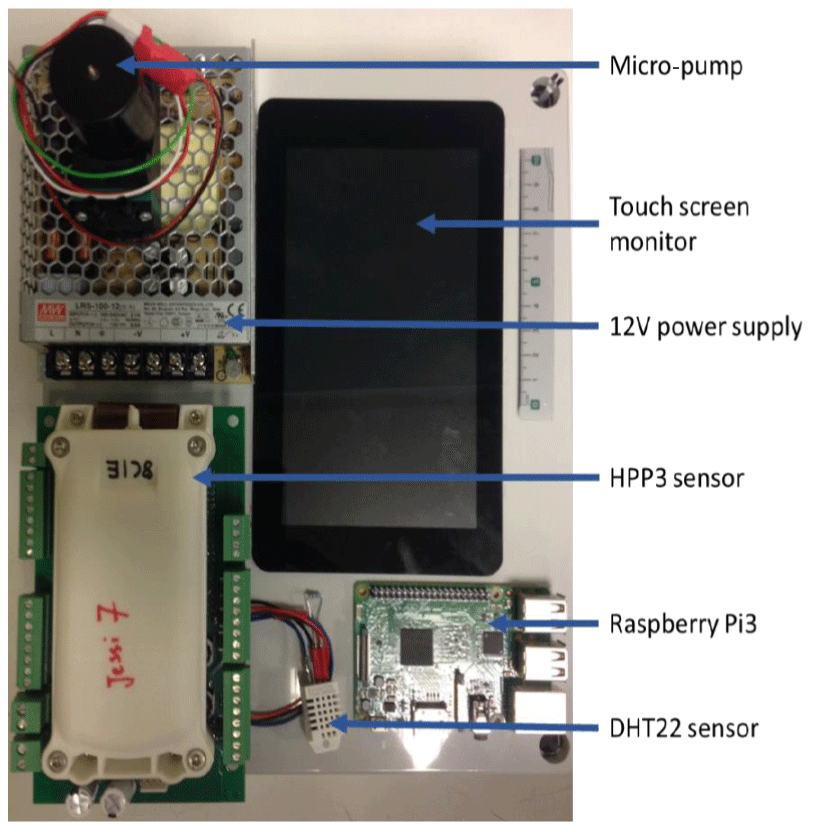
The HPP3 sensors were integrated into a custom-built portable unit, which we will refer to as the instrument. This instrument should be suitable to perform in situ CO2 measurements on ambient air. The instrument is composed of the HPP3 CO2 sensor and temperature (T) and relative humidity (RH) sensors. To be able to continuously flush the measurement cell a diaphragm micro-pump with a built-in potentiometer (Gardner Denver Thomas, USA, model 1410VD/1.5/E/BLDC/12V) was added upstream of the HPP3's optical cell. Temperature and RH were measured at the exterior of the optical cell where gas is released into the surrounding enclosure. For humidity and temperature, a DHT22 sensor kit (Adafruit, USA) was added and connected through an I2C interface. The accuracy of the sensor is ± 2 %–5 % RH and ± 0.5 ∘C. Its range is 0 % RH–100 % RH and −40 to +80 ∘C, respectively. The response time for all sensors was less than 1 min (which is the time step to which data were integrated).
A Raspberry Pi3 (RPi3) (Raspberry Pi Foundation, 2015) is used to collect the data of all sensors. The RPi3 is a small (85×56 mm2) single-board computer running Raspbian OS, an open-source GNU/Linux distribution. The HPP3 sensors were connected via USB. A 7 in. touch screen monitor is connected via an adapter board, which handles power and signal conversion. The package is powered by a switching power supply providing 12 V, but can also be run on a 12 V battery pack. An image of the components of the portable instrument package is available in Fig. 1.
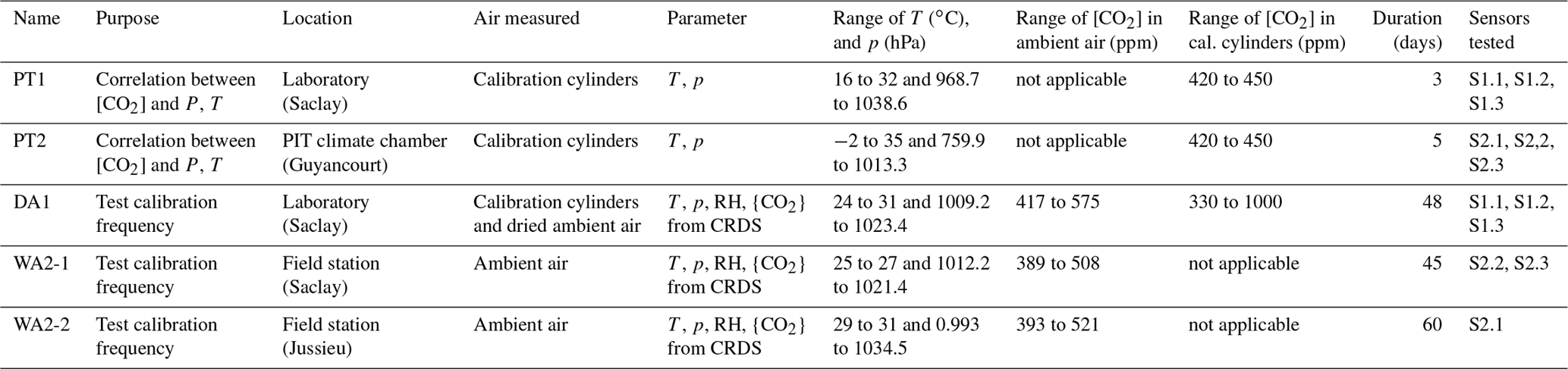
NDIR sensors are sensitive to IR light absorption by CO2 molecules in the air contained in their optical cell, but the retrieval of CO2 dry air mole fraction to the desired uncertainty of 1 ppm is made difficult by sensitivities to temperature, pressure and humidity. Therefore, these parameters should be controlled as much as possible, and their sensitivities characterized, to correct and calibrate reported {CO2}. A series of tests were carried out to characterize the HPP3.1 (S1.1, S1.2, S1.3) and HPP3.2 (S2.1, S2.2, S2.3) performances and sensitivities to {CO2}, T, p and RH. Firstly, temperature, pressure and {CO2} sensitivities were determined in laboratory experiments. Then, field measurements were conducted with an accurate CRDS instrument (Picarro, USA, G2401) measuring the same air as the HPP3 sensors. The CRDS short-term repeatability is estimated to be below 0.02 ppm and the long-term repeatability to be below 0.03 ppm (Yver-Kwok et al., 2015). Table 1 summarizes all laboratory tests and field test measurements, which are presented in this section.
3.1 Laboratory tests
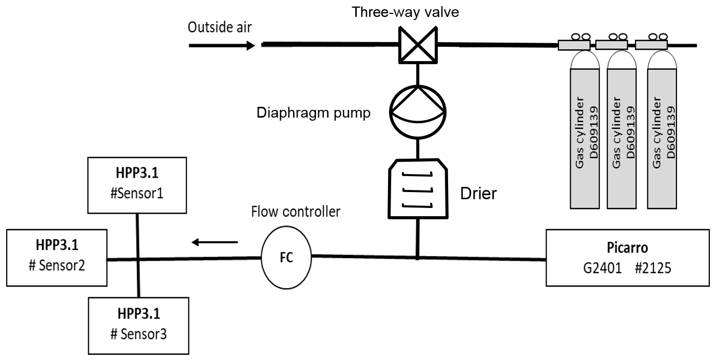
All laboratory tests used the same fundamental setup shown in Fig. 2 with only slight modifications. A diaphragm pump (KNF Lab, Germany, model N86KN.18) was used to pump air from either an ambient air line or calibration cylinders to a Nafion dryer (Perma Pure, USA, MD-070 series), to eliminate H2O traces in the gas line. A flow controller (Bronkhorst, France, El-Flow series) was used to regulate the airflow distributed with a manifold to the HPP3 instruments at 500 mL min−1 to ensure stable experimental conditions while a CRDS instrument could also be connected through a gas split to measure the same air.
3.1.1 Sensitivity to temperature and pressure variations
To assess the linearity of the response of each sensor to {CO2} for different pressure and temperature conditions, two series of temperature and pressure sensitivity tests (PT1, PT2) were realized in a closed chamber with controlled T and p for the HPP3.1 and HPP3.2 sensors. No dryer was necessary as dried air from high-pressure cylinders was used. The CRDS instrument (Picarro, G2401, serial number 2125) was not connected during these tests.
In test PT1 (Table 1), three HPP3.1 sensors were put in a simple plastic chamber and exposed to pressure changes ranging from 977.8 to 1038.6 hPa, and temperature ranges of 16 to 32 ∘C, while measuring gas from a calibration cylinder. Pressure and temperature were measured by a high-precision pressure sensor (Keller, Germany, series 33x, 0.2 hPa and 0.05 K precision).
In test PT2, to test wider ranges for pressure and temperature that might be experienced during field measurements, three HPP3.2 sensors were placed inside a dedicated temperature and pressure chamber at the Plateforme d'Intégration et de Tests (PIT) at OVSQ Guyancourt, France, where a much larger range of T and p variations could be applied. During each T and p test, four calibration cylinders with dry air CO2 dry air mole fractions from 420 to 450 ppm were measured by all the HPP3.2 sensors for a period of approximately 120 h for each cylinder. In the PIT chamber, temperature was varied from −2 to 35 ∘C with a constant rate of change of 1 ∘C h−1, keeping pressure constant at a value of 1013.25 hPa. During pressure tests the chamber pressure was varied from 1013.25 to 759.94 hPa with a decrement of 50.66 hPa, regulated with a primary pump, with temperature fixed at 15 ∘C.
3.1.2 Correction and calibration of CO2 measurements for dry and wet air
These experiments were performed to evaluate the response of HPP3 sensors to {CO2} changes in ambient air. Corrections were established to allow compensation for unintended instrument behaviour and sensitivities, while calibrations are applied to translate the instrument readings to the WMO GAW CO2 scale (here, XCO2 2007). Both steps are combined into one procedure. Two modes of operation for the HPP3 sensors have been tested, i.e. using a dried or an undried gas stream, as those are two common modes of operation in greenhouse gas measurements in different local, regional and global networks (GAW report 242).
3.1.3 Dry air experiments
Water vapour is known to interfere with CO2 measurements, in particular for NDIR sensors. It is thus important to determine the response of the sensors to {CO2} under the best possible conditions, that is, dry air. The experimental setup shown in Fig. 2 was used. In test DA1 (Table 2) different HPP3 sensors were flushed with the same dry ambient air, passed through a Nafion dryer. CRDS measurements were used to monitor and confirm that H2O was reduced to trace amounts, i.e. 0.05±0.05 % H2O. HPP3.1 sensors S1.1, S1.2 and S1.3 were tested extensively for 45 d, and HPP3.2 sensors S2.1 and S2.2 were tested for 12 d.
Additionally, for a period of 45 d during spring 2016, S1.1, S1.2 and S1.3 measurements of dry ambient air in parallel with a co-deployed CRDS instrument (Picarro, USA, G2401) were conducted at the Saclay field site (see Sect. 3.3.1) There ambient air was pumped from a sampling line fixed on the roof of the building (ca. 4 m a.g.l.) to flush the setup described in Fig. 2. Four dry air calibration cylinders (330, 375, 445 and 1000 ppm of {CO2}) were measured once every 13 h; they were sampled successively each for 30 min (Fig. 3). As the HPP3 responses can be slow and in order to remove memory effects, only the last 15 min of each measurement period was used.
3.1.4 Undried (wet) air experiments
As drying is impractical for some applications, we also measured the HPP3's sensitivities to water vapour in undried ambient air and calibration cylinders. If these sensitivities were stable over time, they could be used to correct reported {CO2} for the H2O interference. For WA2-1 and WA2-2 tests, the Nafion dryer was removed from the setup. The only modification of the experiment was the removal of the Nafion dryer.
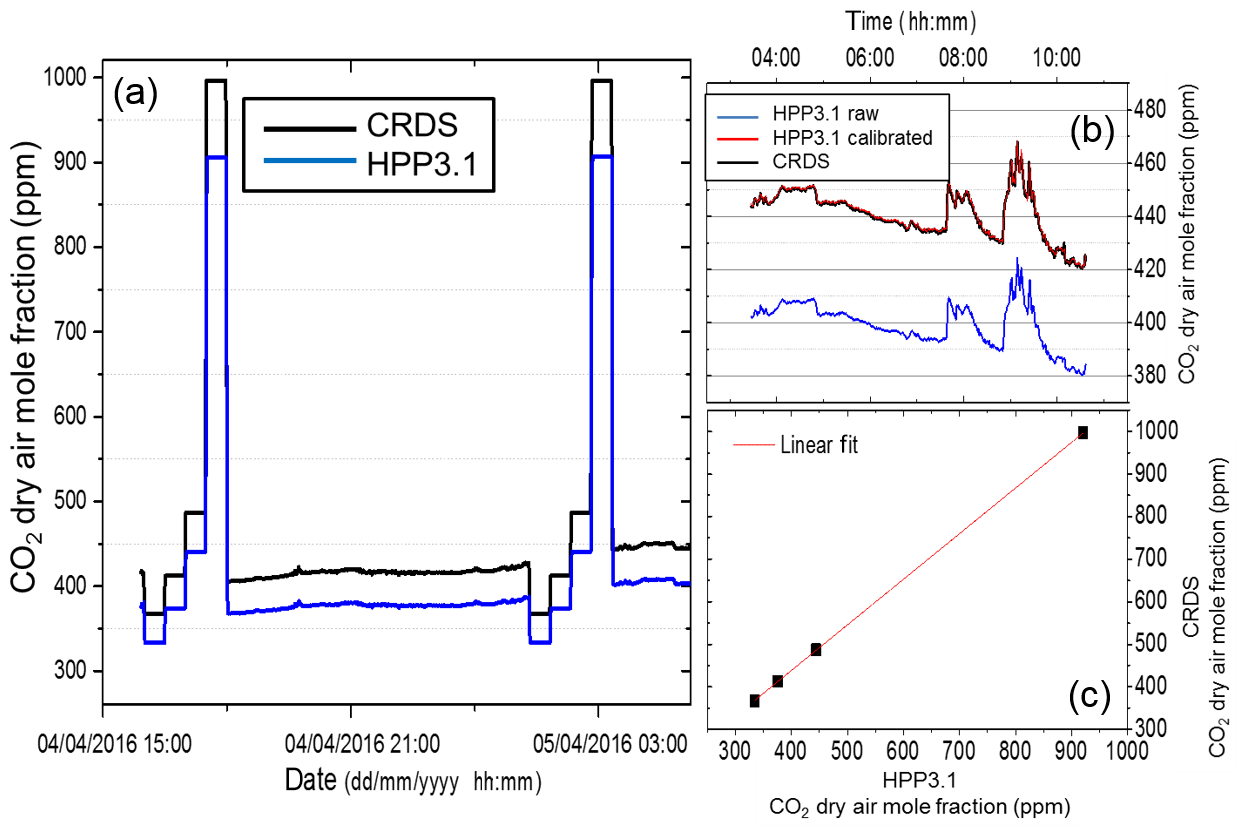
Figure 3(a) CO2 dry air mole fractions measured by S1.1 (blue) and the Picarro CRDS analyzer (black). (b) Calibrated dry air mole fractions of S1.1 (red) compared to the raw values (blue). (c) Four reference gases (assigned values are 367, 413, 487 and 997 ppm of {CO2}) are used for the calibration. No saturation effects are observed within our CO2 dry air mole fraction range.
3.2 Instrument correction and calibration procedure
In order to correct the reported {CO2} we have to define a function that allows us to correct for unintended instrument sensitivities, i.e. to p, T and H2O, as well as to correct {CO2} measurements to an official scale should they show any offset or non-linear behaviour.
3.2.1 Linearity of instrument response
For dry air measurements in test DA1, a linear calibration curve was found to be appropriate. Figure 3c shows that the response of the HPP3 instruments to CO2 dry air mole fraction is linear (R2=0.95) from 330 to 1000 ppm. No saturation effects are observed within this CO2 dry air mole fraction range since residuals are included in the ±1 ppm range. Therefore, a linear response to {CO2} is assumed further on.
3.2.2 Multivariable correction and calibration
Due to the high correlation of air temperature and water vapour content, which were both found to be linear (see Sect. 4), we suggest a multivariable regression method, which includes pressure, temperature and humidity. Indeed, if variables are corrected one at a time, an overcorrection of one of the correlated variables may occur.
Multivariable regression is a generalization of linear regression by considering more than one variable. We used a multivariable linear regression of the form
{CO2}calibrated, corrected corresponds to the measured {CO2} by the reference instrument (CRDS) calibrated on the WMO CO2 X2007 scale. C is the {CO2}HPP3 reported by the HPP3 instrument, with additional factors to capture the influence of the pressure p, the temperature T, the water mixing ratio W (as calculated from our T, p and RH measurements), the baseline drift d and a baseline offset b. All instrument-specific coefficients for the multivariable linear regression are determined using measurements of the parameters for several days.
3.3 Field tests with urban air measurements
To assess their real-world performance, we conducted additional tests for the HPP3 sensors measuring ambient air at two field sites under typical conditions for urban air monitoring. After the sensors were fully integrated into instruments as described in Sect. 2.2. Three HPP3.1 instruments (S1.1, S1.2, S1.3) and two HPP3.2 instruments (S2.2, S2.3) were installed at the Saclay field site (48.7120∘ N, 2.1462∘ E) to measure ambient air on top of the building roof. Saclay is located 20 km south of the center of Paris in a less-urbanized area. In addition, one HPP3.2 instrument (S2.1) was installed to measure air at the Jussieu field site on the Jussieu University campus in the center of Paris (48.8464∘ N, 2.3566∘ E).
3.3.1 Saclay field site tests
The sampling line, a 5 m Dekabon tube with an inner tube diameter of 0.6 cm, was fixed on the rooftop of the building at about 4 m a.g.l., which was connected to a setup that was a copy of the laboratory tests. However, up to five HPP3 instruments were connected and a pump of the same build as in the previous experiments was used to regulate the air-flow distributed with a manifold to the HPP3 instruments at 500 mL min−1 to ensure stable experimental conditions. The field site is equipped with a cooling and heating unit that was turned off most of the time so that room temperature varied between 24 and 31 ∘C. During the test of HPP3.2 for 45 d, four reference gas cylinders (330, 375, 445 and 1000 ppm of CO2) were used and each HPP3 was flushed every 12 h for 30 min per cylinder during the dry air experiment. No calibration cylinders were used during the undried air experiment since the calibration was based on the co-located high-precision measurement with the CRDS analyzer. The mean dry air mole fraction of ambient CO2 was 420 ppm and varied between 388 and 575 ppm during dry air experiments, and a mean of 409 ppm and variations between 389 and 509 ppm were found during the undried air experiments.
3.3.2 Jussieu field site tests
The measurements were conducted at the OCAPI (Observatoire de la Composition de l'Air de Paris a l'IPSL) field station. The measurements from the HPP3.2 instrument (S2.1) in Jussieu were compared with those of a co-located CRDS analyzer (Picarro, USA, G2401). Two independent sampling lines (about 5 m Dekabon tube with an inner tube of 0.6 cm) were used for the CRDS and the S2.1 instrument. The airflow into S2.1 was regulated by the micro-pump (see Sect. 2.2) and set to 500 mL min−1 using a potentiometer. At this location neither a calibration cylinder nor a drying system was deployed for S2.1, but they were calibrated using the CRDS instrument. The measurement period was 60 d and the mean ambient CO2 dry air mole fraction was 410 ppm and minute averages varied between 393 and 521 ppm. Room temperature varied between 28 and 31 ∘C during the observation period.
4.1 Sensitivity to temperature and pressure variations using dried air
4.1.1 HPP3.1 instruments tested in the simple chamber (PT1)
Linear relationships are observed between reported CO2 dry air mole fractions and p and T (R2=0.99 with p and R2=0.92 with T) in the simple chamber (see Figs. 4 and 5). Due to the limitation of experimental conditions in these simple plastic chambers, only a narrow pressure range of 977.78 to 1033.52 hPa and a temperature range of 16 to 32 ∘C could be tested for these instruments. Different slopes and intercepts are found for each instrument as reported in Table 2. This indicates that there is no single universal p and T calibration curve that could be determined for one instrument and used for others.
4.1.2 HPP3.2 instruments tested in the PIT chamber (PT2)
The PT2 test results with pressure changes from 1013.25 to 759.94 hPa with an increment of 50.66 hPa are shown in Fig. 4. Figure 4 shows the variations in CO2 dry air mole fractions due to p changes (from 0.0049 to 0.0177 ppm hPa−1). Despite the built-in pressure compensation algorithm developed for HPP3.2, reported {CO2} and p can still co-vary with a positive (S2.1 and S2.2) or a negative (S2.3) correlation, indicating that an additional correction is required when aiming to achieve the best possible results (see also Fig. S1 in the Supplement). Consequently, we applied a linear fit between Δ{CO2} (differences between the assigned dry air mole fraction in the cylinder and the dry air mole fraction reported by HPP3.2 instruments) and pressure (Fig. 6). The slope and intercept obtained are then used to determine the offset due to p variations that has to be added to {CO2} reported by the HPP3.2 instruments. The corrected {CO2} values have a root-mean-square deviation from the assigned dry air mole fraction in the calibration cylinder (428.6 ppm) of less than 0.02 ppm for all three HPP3.2 instruments (see also Fig. S2). Figure 5 shows the effect of temperature variations in the PIT chamber ranging from −2 to 35 ∘C (see Sect. 3.1) on reported CO2 dry air mole fractions of the HPP3.2 instruments. For the three HPP3.2 instruments, {CO2} is negatively correlated to T. As for the tests in the simple chamber with the HPP3.1 instruments, different linear T slopes and intercepts are observed for each HPP3.1 instrument (Fig. 5) in the PIT chamber. After correction for temperature variations, we obtain corrected {CO2} values with a root-mean-square deviation which does not exceed 0.01 ppm from the assigned value of the cylinder (444 ppm) for the three HPP3.2 instruments (see also Fig. S3).
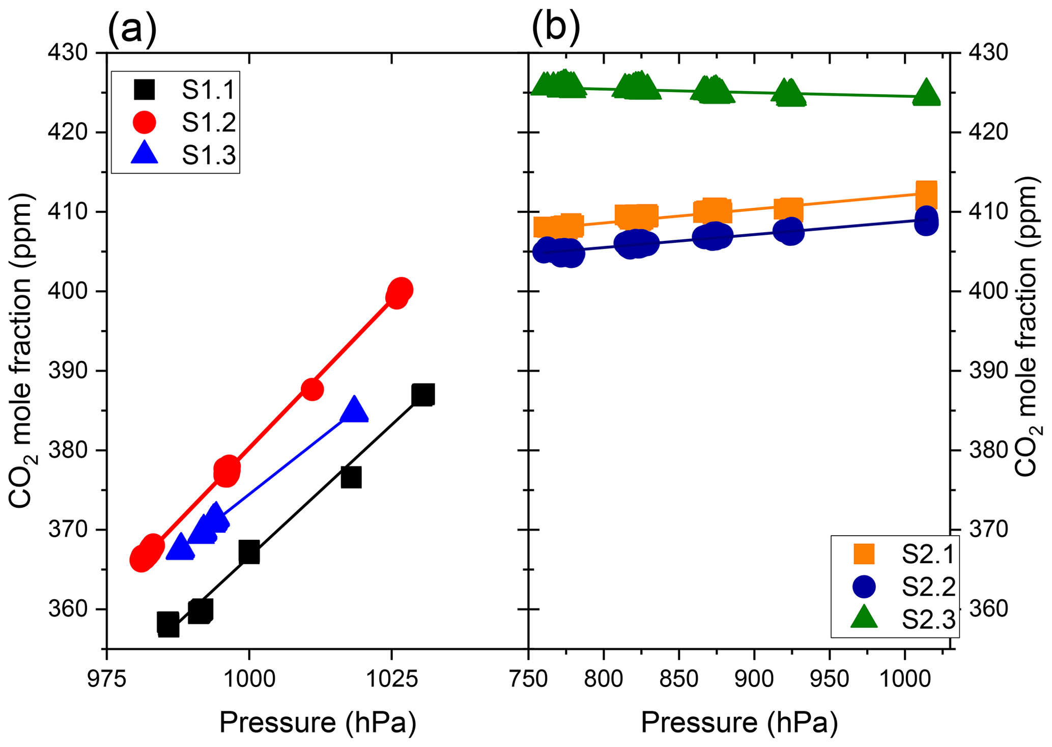
Figure 4Linear relationship experimentally found between reported {CO2} and p for S1.1, S1.2 and S1.3 (a) and for the instruments S2.1, S2.2 and S2.3 (b). Note the different p range, ranging from 972.7 to 1030 hPa for the HPP3.1 instruments in the simple plastic chamber and 759.9 to 1013.25 hPa for the HPP3.2 instruments in the PIT chamber.
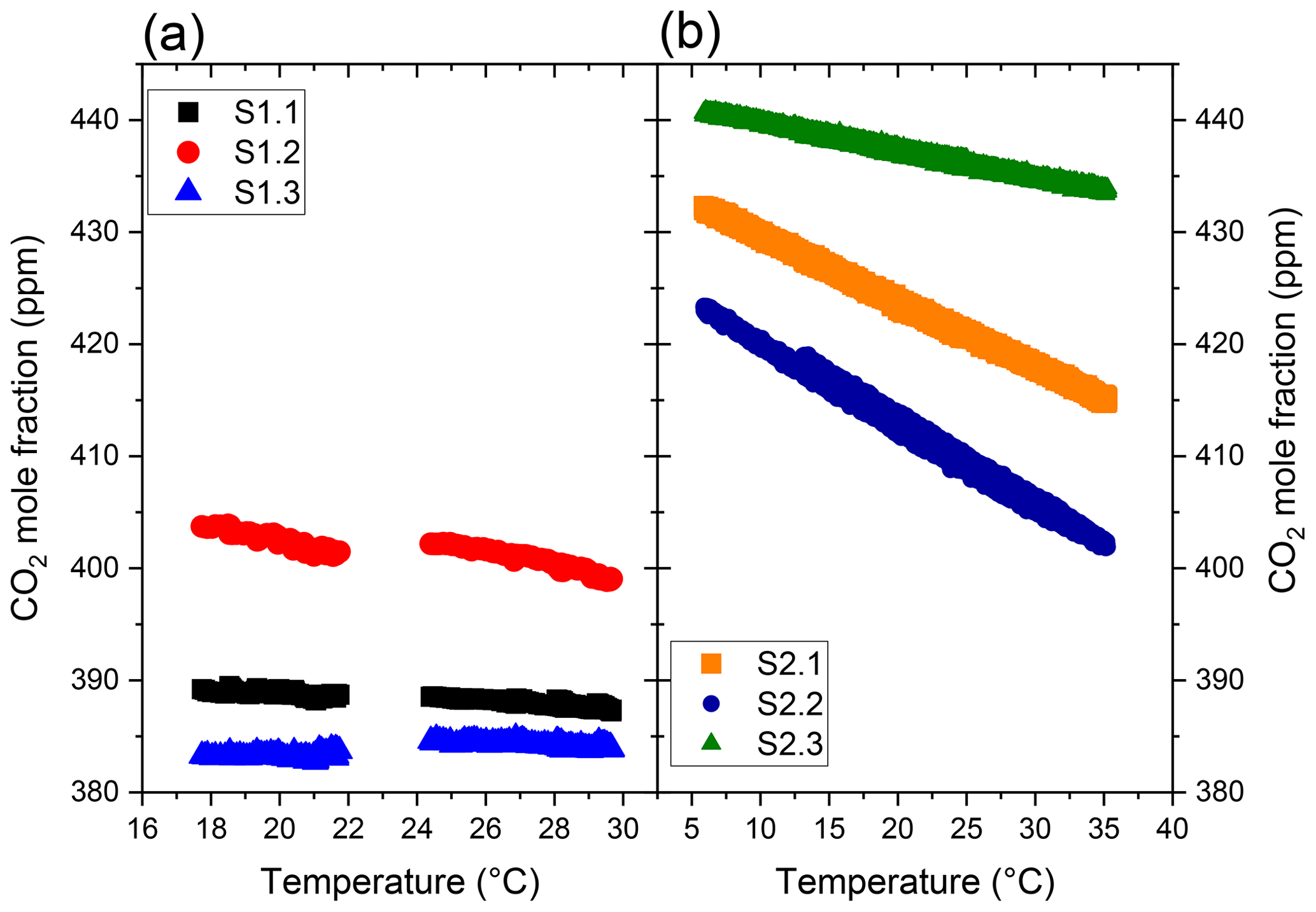
Figure 5Linear relationships between reported {CO2} for S1.1 S1.1, S1.2 and S1.3 (a) at temperature values ranging from 17 to 30 ∘C in the plastic chamber, and for S2.1, S2.2 and S2.3 at temperature values ranging from 5 to 35 ∘C in the PIT chamber (b).
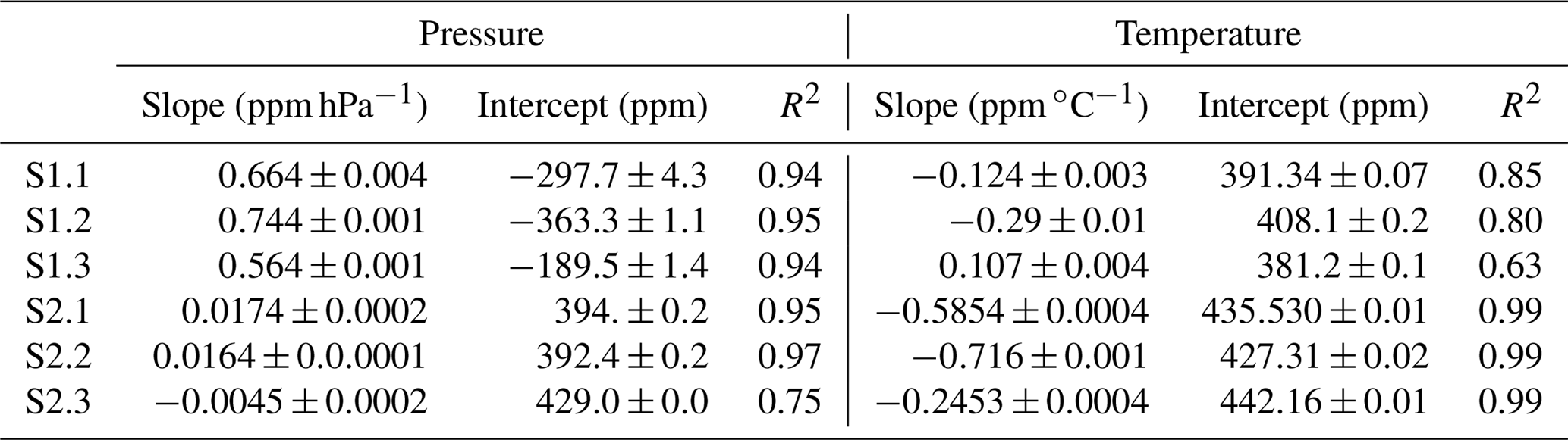
Table 2 summarizes the results of the pressure and temperature tests for all instruments. These test results show a sensor-specific response to p and T. A large difference of reported {CO2} sensitivity to pressure variations is observed between the two HPP3 versions. A sensitivity of 0.564 to 0.744 ppm hPa−1 is found for the HPP3.1 sensors, whereas this sensitivity ranges from −0.0045 up to 0.0174 ppm hPa−1 for the newer HPP3.2 sensors. The lower sensitivity among HPP3.2 prototypes is due to the pressure compensation algorithm, which is included in this model. Since the pressure compensation algorithm still does not fully correct the reported {CO2} variations due to pressure changes, we found that it is necessary to apply a correction for pressure, and this correction should be sensor specific. The {CO2} sensitivity to temperature variations is found to be in a similar range for both sensor makes. Sensitivities of −0.3 to 0.1 and −0.2 to −0.7 ppm ∘C−1 are found for the HPP3.1 and HPP3.2 instruments, respectively.
Table 2Slopes and intercept calculated for CO2 correction due to temperature and pressure. Sensors S1.1 to S1.3 are type HPP3.1, whereas sensors S2.1 to S2.3 are HPP3.2.
After applying our correction for temperature and pressure, no more correlations are observed between corrected {CO2} and pressure and temperature. Corrected CO2 mole fractions of HPP3.2 are stable and standard errors do not exceed 0.3 and 0.2 ppm for pressure and temperature corrections respectively, except for {CO2} after temperature correction for S2.2, which reaches a standard deviation (SD) of 0.5 ppm. However, we do not reach the same stability after pressure and temperature correction for HPP3.1 prototypes. Standard deviations of 0.9, 0.2 and 0.2 ppm are calculated for S1.1, S1.2 and S1.3 respectively after pressure correction, and standard deviations of 1.3, 2.6 and 1.6 ppm are determined for S1.1, S1.2 and S1.3 respectively after temperature corrections. These differences between the results of the two HPP3 versions can be partly explained by the fact that HPP3.2 prototypes had the opportunity to be tested in a sophisticated climatic chamber which respects precise temperature and pressure set points for more longer-term measurements and in which only one of the two variables is modified at a time.
4.2 Instrument calibration and stability during continuous measurements
Our instrument described in this study is intended for use in field campaign studies and longer-term monitoring. We assess its performance during continuous measurements. We also evaluate which calibration frequency is necessary to track the changes in the sensitivities to p and T found in Sect. 4.1 and if the instruments can be calibrated when using an undried gas stream. Given that the instrument response to {CO2} is also affected by atmospheric water vapour, we present the results from dried and wet ambient air measurements separately.
4.2.1 Measurements of dried ambient air (DA1)
Four calibration cylinders were used in order to calibrate the three HPP3.1 instruments (see Sect. 3.1). To assess the quality of this calibration, the mean and standard deviation (SD) of Δ{CO2} (i.e. {CO2}HPP3 minus {CO2} CRDS) of 1 min averaged data were calculated and are shown in Fig. 6. Although calibration cylinders were measured each 12 h, by ignoring some calibration data, we processed the time series to recompute calibrated {CO2} assuming a range of different time intervals between two calibrations. The results shown in Fig. 6 are for calibration intervals of 0.5, 6, 12, 19, 25, 31, 38 and 45 d. Each point in this figure corresponds to the values calculated for the instruments S1.1, S1.2 and S1.3.
We find that the 1 ppm repeatability threshold is nearly met when measuring dried air for calibration intervals of 6 d. The SD Δ{CO2} of the minute averages slowly increases with increasing calibration intervals but seems to stabilize between 3 and 4 ppm. We also see a marked difference between the performances of each sensor: S1.1 shows the best performance, followed by S1.3 and S1.2. In addition to an increased SD, we also see that the mean of Δ{CO2} increases significantly after not calibrating for 19 d. Surprisingly, one calibration each 45 d does not seem to deteriorate the mean of Δ{CO2} further. In fact, the mean Δ{CO2} seems to decrease over longer time periods.
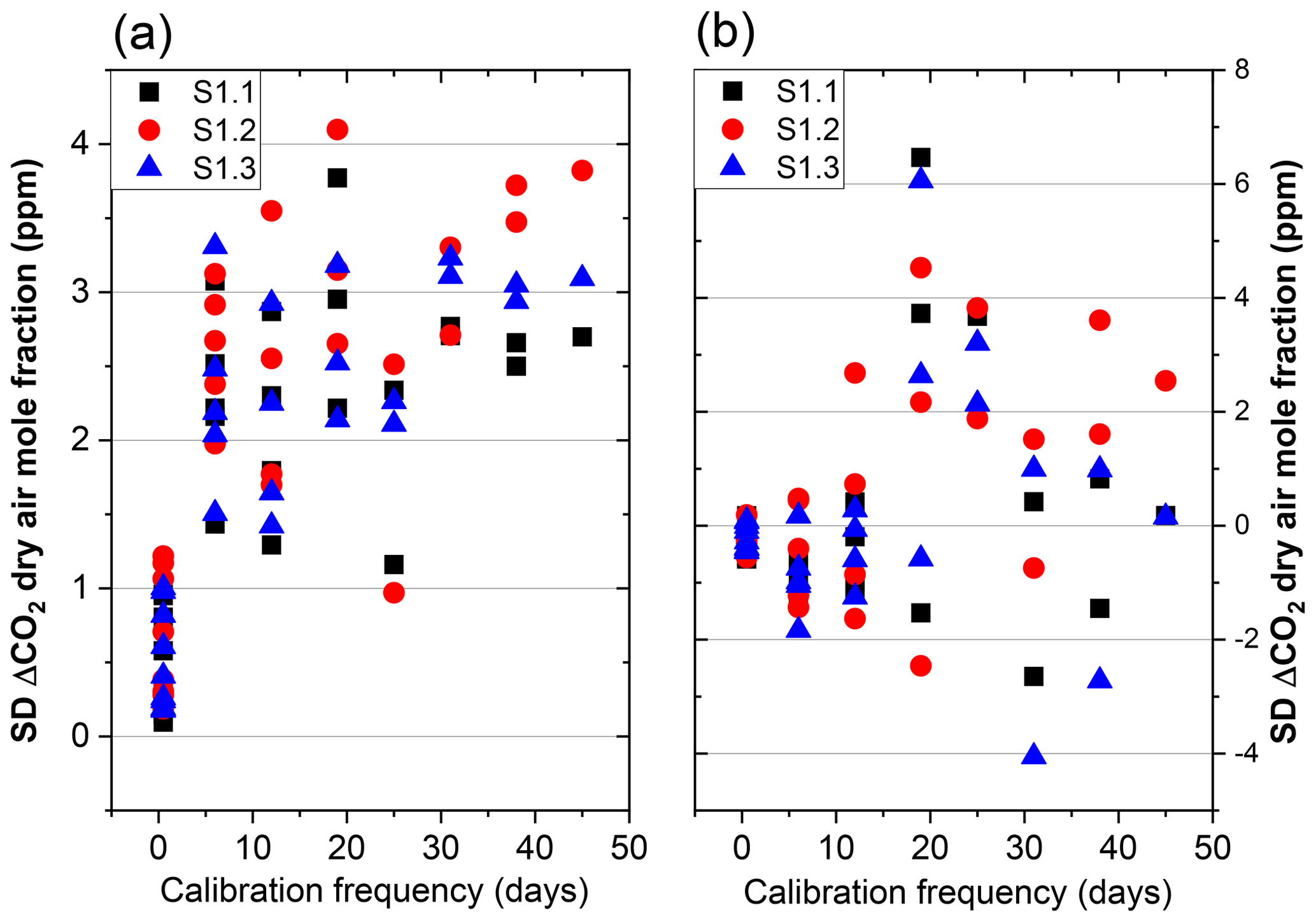
Figure 6SD (a) and mean (b) values of the 1 min average of mean Δ{CO2}, during a measurement period of 48 d depending on the calibration frequency.
4.2.2 Saclay ambient air measurements (WA2-1)
During this test (Sect. 3.3.1), {CO2} and variables affecting the instrument stability, i.e. pressure, temperature and water vapour content were measured from 20 July until 8 August. The meteorological parameters during the field campaign are given in Fig. S4. Our previous measurements already indicated that regular recalibration of the HPP3 instruments is required because of sensitivities to T, p and water vapour that are instrument specific and time dependent. We call the period during which the six calibration coefficients of Eq. (1) are calculated by using the CRDS {CO2} time series the calibration period. Attempting to determine those calibration coefficients during a short calibration period, e.g. of 1 week, leads to high mean Δ{CO2}, as can be seen in Fig. 7. A calibration period of 2 weeks leads to significantly better results. We benchmark the instrument performance for both minute averages, the instruments' typical temporal resolution, and hourly averages, as those are widely used in modelling studies and data assimilation systems.
We also compared different calibration periods of the same length. As an example, considering a 45 d experiment, we chose three different calibration periods of successive 15 d. We also tested the approach of using the first and last weeks of a 45 d period to create a non-successive two-week calibration period.
Figure 7a, b show the SD and mean Δ{CO2} values considering three calibration periods (C1, C2, C3) of 15 d each. The regression coefficients of the multivariable model of Eq. (1) for C1, C2 and C3 are calculated using the first, second and third consecutive 15 d of the experimental period. These coefficients are then used to predict corrected {CO2}HPP3 for the three cross-validation periods of 15, 30 and 45 d. Also, calibration coefficients (W1, W6) were calculated using the first and sixth weeks of the 45 d period for calibration. Unsurprisingly, using C1 coefficients gives the best results for the first 15 d used for training, and lead a higher bias for the last 15 d. Using C2 coefficients to correct the 15 d adjacent to the calibration period gives comparable results. Considering the last calibration period, C3 coefficients show a mean bias of −2.5 ppm when calibration is from the first 15 d. One reason that can explain this behaviour is the greater variability of CO2 dry air mole fraction during the last 15 d of the experiment. The interquartile range of CO2 dry air mole fraction is 10, 15 and 25 ppm respectively for the first, second and third periods. The CO2 dry air mole fraction correction is accomplished mostly by correcting T, P, H2O and the instrument offset. A small variation in sensitivities may lead to a less appropriate correction for periods of smaller variability. Another reason for this difference is the drift component of the correction in Eq. (1). The linear drift of the instrument also varies with time. One method to better correct for the slow linear drift of the instrument is to combine the first and last weeks of the experiment into a calibration period instead of using 2 consecutive weeks. When using the first week (W1) and the last week (W6) for calibration, the instrument drift is not properly corrected and a residual linear drift of 0.14 and 0.28 ppm week−1 is visible in the black (W1) and the red (W6) curves of Fig. S5 respectively. Nearly no drift (0.01 ppm week−1) is observed when considering both W1 and W6 for the training (blue curve). In Fig. 7, magenta stars show SD Δ{CO2} and mean Δ{CO2} values of the whole 45 d time series considering both W1 and W6 as calibration periods. With this coefficient determination method, mean ΔCO2 bias can be reduced to nearly 0 ppm. Finally, we should note that averaging the 1 min data to hourly averages can further improve SD Δ{CO2} values up to 28 %. As expected, mean values do not change for hourly averages.
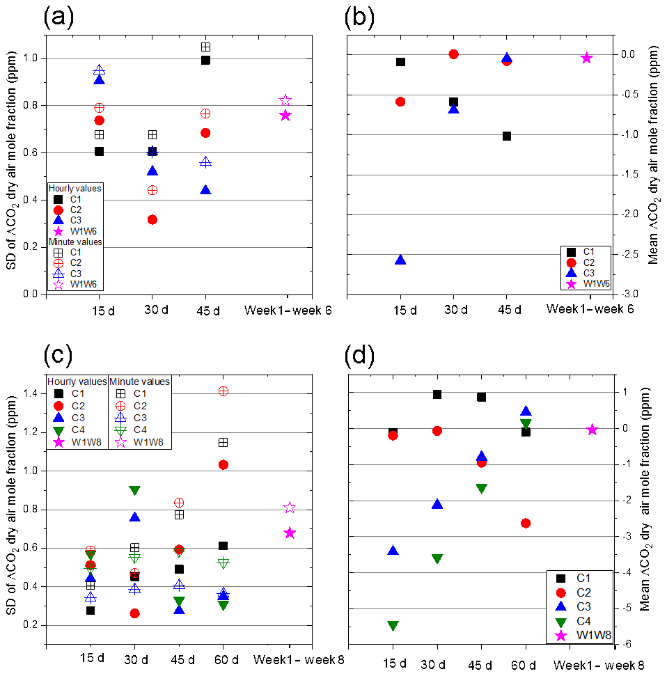
Figure 7SD Δ{CO2} (a) and mean Δ{CO2} (b) values considering three calibration periods of 15 consecutive days for calibration each, with C1, C2 and C3 corresponding to the first, second and third 15 consecutive days of measurements at the Saclay field site respectively. W1W6 corresponds to using the first and sixth weeks as the calibration period. Mean ΔCO2 calculated for the four calibration periods. SD Δ{CO2} (c) and mean Δ{CO2} (d) values considering four calibration periods of 15 consecutive days for calibration each, with C1, C2, C3 and C4 corresponding to the first, second, third and fourth 15 consecutive days of measurements at the Jussieu field site respectively. W1W6 corresponds to using the first and eighth weeks as the calibration period. Hourly and minute values are represented as full and empty symbols respectively.
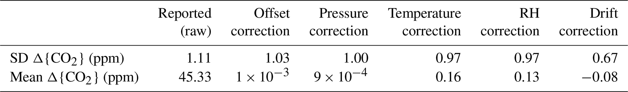
Furthermore, we can investigate which of the six term multivariable linear regressions is most important here. The offset correction terms and correction terms depending on dry air mole fraction (b and {CO2}HPP3) are the most significant corrections among all five parameters and allow the reduction of the mean ΔCO2 from 45 to 0 ppm (see Table 3 and Fig. S3). The other four parameters (pressure, temperature, water vapour and drift corrections) further reduce the difference between CRDS and HPP3.2, reducing the SD Δ{CO2} of minute averages from 1.03 to 0.67 ppm. Here, the temperature correction (d) and the water vapour correction (e) provide a correction of similar magnitude, keeping the same SD and improving mean Δ{CO2} only from 0.16 to 0.13 ppm. This is understandable since temperature and water vapour are correlated for this type of measurement.
Table 3SD and mean values of 1 min average Δ{CO2} data for each correction step. Note that corrections are cumulative from left to right.
4.2.3 Jussieu ambient air measurements (WA2-2)
To assess the further performance of the HPP3.2 instruments, additional wet ambient air measurements at the second field site in Jussieu were carried out for 60 consecutive days using instrument S2.1 alongside a CRDS instrument. Figure 7c, d show SD Δ{CO2} and mean Δ{CO2} values calculated with four calibration periods of 15 consecutive days each and one calibration considering both the first and last weeks of the experiment. Calibration coefficients for C1, C2, C3 and C4 are calculated considering calibration periods of the first, second, third and fourth 15 consecutive days of the experiment respectively. W1W8 coefficients are calculated considering week one (W1) and week eight (W8) of the experiment. The results are qualitatively very similar to the measurements at the Saclay field site, and combing the first and last weeks as calibration period also results in achieving our target of SD Δ{CO2} > 1 ppm.
We integrated HPP3.1 and HPP3.2 NDIR sensors into a portable low-cost instrument with additional sensors and internal data acquisition. The laboratory tests reveal a strong sensitivity of reported CO2 dry air mole fractions to ambient air pressure for the HPP3.1 series and a significantly decreased, yet noticeable, sensitivity to pressure, for the upgraded HPP3.2 sensors equipped with the built-in manufacturer p correction. To achieve the targeted stability (long-term repeatability) for urban observations of 1 ppm or better, instruments have to be corrected at regular intervals against data from a reference instrument (here CRDS) to account for their cross-sensitivities to (H2O mixing ratio) changes and electronic drift, unless those parameters could be controlled externally in the future. We found that commercially available p, T and RH sensors that are compatible with the chosen Raspberry Pi3 platform are sufficiently precise to use these parameters as predictors of the linear equation used to calibrate each HPP3 instrument against the reference instrument, which was calibrated to the official WMO CO2 X2007 CO2 scale.
Two common modes of operation have been successfully tested, i.e. using the HPP3 instruments for either dried or undried ambient air measurements. Our results indicate that using a dried gas stream does not improve measurement precision or stability compared to an undried gas stream provided that a multivariable regression model is used for calibration, which accounts for all cross-sensitivities including H2O mixing ratio changes.
We furthermore find that sensor-specific corrections are required and they should be considered time dependent, e.g. by including a linear drift that only becomes more apparent for longer-term observations. Different calibration windows were tested for both the Saclay field site and Jussieu field site ambient air measurements and their results were evaluated against CRDS data that were not used for calibration. Those sites exhibit the typical {CO2} levels in urban GHG monitoring networks where future low-cost medium-precision instruments could be deployed. Regular (6-weekly) recalibrations are found to be appropriate to capture sensor drifts and changes in relevant cross-sensitivities, while not increasing the burden of performing calibration too often. A dedicated set of calibration gases was not necessary if the low-cost instrument was calibrated against {CO2} from a CRDS instrument using the same air. Calibration periods of 1 week with parallel CRDS measurements before and after a 45 d deployment were sufficient for the SD Δ{CO2} data to be within 1 ppm of the CRDS measurements during that period (with near-zero bias, i.e. Δ{CO2} ≪1 ppm). This calibration approach can thus be an alternative to permanently deploying calibration gases for each individual sensor.
The field tests at the Saclay and Jussieu stations are being continued to see if the instrument performance deteriorates over its lifetime. Since the start of the test in 2015 until now, multiple HPP3.1 sensors have been in use without significant performance loss. Other research groups have also started integrating HPP sensors into their low-cost GHG monitoring strategy (e.g. Carbosense, http://www.nano-tera.ch/projects/491.php, last access: 11 March 2019).
Future improvements for the LCMP instruments will include the addition of batteries to allow their transport to the central calibration lab without power cut as well as using them in field campaigns, e.g. landfills when connected to solar panels or small wind turbines. During future tests at sites without reference instruments, small pressurized gas containers (12l, minican, Linde Gas) will be used to regularly inject target gas to track the performance during a deployment period.
The overall operational cost of the new calibration scheme using a central laboratory and rotating the LCMP systems can also only be assessed after more extensive field deployment has been performed.
The Python scripts for the data collection from the HPP3 and DHT22 for Raspberry Pi 3, and the data from the experiments described here are available from the corresponding authors upon request.
The supplement related to this article is available online at: https://doi.org/10.5194/amt-12-2665-2019-supplement.
The first authors EA and FRV conducted the measurements reported in this study and planned the work with support of PC. AB and BG supported the development of the data logging routine and processing scripts. OL and MR supported measurements by providing access to the ICOS test laboratory equipment and supplied reference gases. The initial draft of the paper was developed by EA, FRV and PC. All authors have updated, contributed and edited the paper.
Bakhram Gaynullin is an employee of Senseair AB, which manufactured the HPP prototypes. The authors declare that they have no conflict of interest.
This article is part of the special issue “The 10th International Carbon Dioxide Conference (ICDC10) and the 19th WMO/IAEA Meeting on Carbon Dioxide, other Greenhouse Gases and Related Measurement Techniques (GGMT-2017) (AMT/ACP/BG/CP/ESD inter-journal SI)”. It is a result of the 19th WMO/IAEA Meeting on Carbon Dioxide, Other Greenhouse Gases, and Related Measurement Techniques (GGMT-2017), Empa Dübendorf, Switzerland, 27–31 August 2017.
We would like to thank the anonymous reviewers and the editor whose comments have helped to significantly improve this paper. The work conducted here was partially funded through the LOCATION project of the Low Carbon City Laboratory and a SME-VOUCHER from Climate-KIC (EIT) as well as the Chaire BridGES of UVSQ, CEA, Thales Alenia Space and Veolia S.A.
This paper was edited by Martin Steinbacher and reviewed by two anonymous referees.
Andres, R. J., Boden, T. A., and Higdon, D.: A new evaluation of the uncertainty associated with CDIAC estimates of fossil fuel carbon dioxide emission, Tellus B, 66, 23616, https://doi.org/10.3402/tellusb.v66.23616, 2014.
Bréon, F. M., Broquet, G., Puygrenier, V., Chevallier, F., Xueref-Remy, I., Ramonet, M., Dieudonné, E., Lopez, M., Schmidt, M., Perrussel, O., and Ciais, P.: An attempt at estimating Paris area CO2 emissions from atmospheric concentration measurements, Atmos. Chem. Phys., 15, 1707–1724, https://doi.org/10.5194/acp-15-1707-2015, 2015.
Broquet, G., Bréon, F.-M., Renault, E., Buchwitz, M., Reuter, M., Bovensmann, H., Chevallier, F., Wu, L., and Ciais, P.: The potential of satellite spectro-imagery for monitoring CO2 emissions from large cities, Atmos. Meas. Tech., 11, 681–708, https://doi.org/10.5194/amt-11-681-2018, 2018.
Cambaliza, M. O. L., Shepson, P. B., Caulton, D. R., Stirm, B., Samarov, D., Gurney, K. R., Turnbull, J., Davis, K. J., Possolo, A., Karion, A., Sweeney, C., Moser, B., Hendricks, A., Lauvaux, T., Mays, K., Whetstone, J., Huang, J., Razlivanov, I., Miles, N. L., and Richardson, S. J.: Assessment of uncertainties of an aircraft-based mass balance approach for quantifying urban greenhouse gas emissions, Atmos. Chem. Phys., 14, 9029–9050, https://doi.org/10.5194/acp-14-9029-2014, 2014.
Eugster, W. and Kling, G. W.: Performance of a low-cost methane sensor for ambient concentration measurements in preliminary studies, Atmos. Meas. Tech., 5, 1925–1934, https://doi.org/10.5194/amt-5-1925-2012, 2012.
GAW report 242: 19th WMO/IAEA Meeting on Carbon Dioxide, Other Greenhouse Gases and Related Measurement Techniques (GGMT-2017), World Meteorological Organization, edited by: Crotwell, A. and Steinbacher, M., available at: https://library.wmo.int/doc_num.php?explnum_id=5456 (last access: 10 February 2018), 2018.
Gaynullin, B., Bryzgalov, M., Hummelgård, C., and Rödjegard, H.: A practical solution for accurate studies of NDIR gas sensor pressure dependence, Lab test bench, software and calculation algorithm, IEEE Sensors, 30 October–3 November, Orlando, FL, 1–3, https://doi.org/10.1109/ICSENS.2016.7808828, 2016.
Holstius, D. M., Pillarisetti, A., Smith, K. R., and Seto, E.: Field calibrations of a low-cost aerosol sensor at a regulatory monitoring site in California, Atmos. Meas. Tech., 7, 1121–1131, https://doi.org/10.5194/amt-7-1121-2014, 2014.
Hummelgård, C., Bryntse, I., Bryzgalov, M., Henning, J.-Å, Martin, H., Norén, M., and Rödjegård, H.: Low-Cost NDIR Based Sensor Platform for Sub-Ppm Gas Detection, Urban Climate, 14, 342–350, https://doi.org/10.1016/j.uclim.2014.09.001, 2015.
Kunz, M., Lavric, J. V., Gerbig, C., Tans, P., Neff, D., Hummelgård, C., Martin, H., Rödjegård, H., Wrenger, B., and Heimann, M.: COCAP: a carbon dioxide analyser for small unmanned aircraft systems, Atmos. Meas. Tech., 11, 1833–1849, https://doi.org/10.5194/amt-11-1833-2018, 2018.
Lauvaux, T., Miles, N. L., Deng, A., Richardson, S. J., Cambal-iza, M. O., Davis, K. J., Gaudet, B., Gurney, K. R., Huang, J.,O'Keefe, D., Song, Y., Karion, A., Oda, T., Patarasuk, R., Razli-vanov, I., Sarmiento, D., Shepson, P., Sweeney, C., Turnbull, J., and Wu, K.: High-resolution atmospheric inversion of urban CO2 emissions during the dormant season of the Indianapolis Flux Experiment (INFLUX), J. Geophys. Res.-Atmos., 121, 5213–5236, https://doi.org/10.1002/2015JD024473, 2016.
Liu, Z., He, C., Zhou, Y., and Wu, J.: How much of the world's land has been urbanized, really? A hierarchical framework for avoiding confusion, Landscape Ecol., 29, 763–771, https://doi.org/10.1007/s10980-014-0034-y, 2014.
Martin, C. R., Zeng, N., Karion, A., Dickerson, R. R., Ren, X., Turpie, B. N., and Weber, K. J.: Evaluation and environmental correction of ambient CO2 measurements from a low-cost NDIR sensor, Atmos. Meas. Tech., 10, 2383–2395, https://doi.org/10.5194/amt-10-2383-2017, 2017.
Mays, K. L., Shepson, P. B., Stirm, B. H., Karion, A., Sweeney, C., and Gurney, K. R.: Aircraft-based measurements of the carbon footprint of Indianapolis, Environ. Sci. Technol., 43, 7816–7823, https://doi.org/10.1021/es901326b, 2009.
Nassar, R., Hill, T. G., McLinden, C. A., Wunch, D., Jones, D. B. A., and Crisp, D.: Quantifying CO2 emissions from individual power plants from space, Geophys. Res. Lett., 44, 10045–10053, https://doi.org/10.1002/2017GL074702, 2017.
Piedrahita, R., Xiang, Y., Masson, N., Ortega, J., Collier, A., Jiang, Y., Li, K., Dick, R. P., Lv, Q., Hannigan, M., and Shang, L.: The next generation of low-cost personal air quality sensors for quantitative exposure monitoring, Atmos. Meas. Tech., 7, 3325–3336, https://doi.org/10.5194/amt-7-3325-2014, 2014.
Raspberry Pi Foundation: Raspberry Pi Hardware Documentation, available at: https://www.raspberrypi.org/documentation/hardware/raspberrypi/, last access: 30 April 2019.
Rella, C. W., Chen, H., Andrews, A. E., Filges, A., Gerbig, C., Hatakka, J., Karion, A., Miles, N. L., Richardson, S. J., Steinbacher, M., Sweeney, C., Wastine, B., and Zellweger, C.: High accuracy measurements of dry mole fractions of carbon dioxide and methane in humid air, Atmos. Meas. Tech., 6, 837–860, https://doi.org/10.5194/amt-6-837-2013, 2013.
Seto, K. C., Dhakal, S., Bigio, A., Blanco, H., Delgado, G. C., Dewar, D., Huang, L., Inaba, A., Kansal, A., Lwasa, S., McMahon, J. E., Müller, D. B., Murakami, J., Nagendra, H., and Ramaswami, A.: Human settlements, infrastructure and spatial planning, in: Climate Change 2014: Mitigation of Climate Change. Contribution of Working Group III to the Fifth Assessment Report of the Intergovernmental Panel on Climate Change, edited by: Edenhofer, O., Pichs-Madruga, R., Sokona, Y., Farahani, E., Kadner, S., Seyboth, K., Adler, A., Baum, I., Brunner, S., Eickemeier, P., Kriemann, B., Savolainen, J., Schlömer, S., von Stechow, C., Zwickel, T., and Minx, J. C., Cambridge, United Kingdom and New York, NY, USA, 2014.
Shusterman, A. A., Teige, V. E., Turner, A. J., Newman, C., Kim, J., and Cohen, R. C.: The BErkeley Atmospheric CO2 Observation Network: initial evaluation, Atmos. Chem. Phys., 16, 13449–13463, https://doi.org/10.5194/acp-16-13449-2016, 2016.
Staufer, J., Broquet, G., Bréon, F.-M., Puygrenier, V., Chevallier, F., Xueref-Rémy, I., Dieudonné, E., Lopez, M., Schmidt, M., Ramonet, M., Perrussel, O., Lac, C., Wu, L., and Ciais, P.: The first 1-year-long estimate of the Paris region fossil fuel CO2 emissions based on atmospheric inversion, Atmos. Chem. Phys., 16, 14703–14726, https://doi.org/10.5194/acp-16-14703-2016, 2016.
Turner, A. J., Shusterman, A. A., McDonald, B. C., Teige, V., Harley, R. A., and Cohen, R. C.: Network design for quantifying urban CO2 emissions: assessing trade-offs between precision and network density, Atmos. Chem. Phys., 16, 13465–13475, https://doi.org/10.5194/acp-16-13465-2016, 2016.
Verhulst, K. R., Karion, A., Kim, J., Salameh, P. K., Keeling, R. F., Newman, S., Miller, J., Sloop, C., Pongetti, T., Rao, P., Wong, C., Hopkins, F. M., Yadav, V., Weiss, R. F., Duren, R. M., and Miller, C. E.: Carbon dioxide and methane measurements from the Los Angeles Megacity Carbon Project – Part 1: calibration, urban enhancements, and uncertainty estimates, Atmos. Chem. Phys., 17, 8313–8341, https://doi.org/10.5194/acp-17-8313-2017, 2017.
Wang, Y., Li, J. Y., Jing, H., Zhang, Q., Jiang, J. K., and Biswas, P.: Laboratory Evaluation and Calibration of Three Low- Cost Particle Sensors for Particulate Matter Measurement, Aerosol Sci. Tech., 49, 1063–1077, https://doi.org/10.1080/02786826.2015.1100710, 2015.
Wu, L., Broquet, G., Ciais, P., Bellassen, V., Vogel, F., Chevallier, F., Xueref-Remy, I., and Wang, Y.: What would dense atmospheric observation networks bring to the quantification of city CO2 emissions?, Atmos. Chem. Phys., 16, 7743–7771, https://doi.org/10.5194/acp-16-7743-2016, 2016.
Young, D. T., Chapman, L., Muller, C. L., Cai, X. M., and Grimmond, C. S. B.: A Low-Cost Wireless Temperature Sensor: Evaluation for Use in Environmental Monitoring Applications, J. Atmos. Ocean. Tech., 31, 938–944, https://doi.org/10.1175/jtech-d-13-00217.1, 2014.
Yver Kwok, C., Laurent, O., Guemri, A., Philippon, C., Wastine, B., Rella, C. W., Vuillemin, C., Truong, F., Delmotte, M., Kazan, V., Darding, M., Lebègue, B., Kaiser, C., Xueref-Rémy, I., and Ramonet, M.: Comprehensive laboratory and field testing of cavity ring-down spectroscopy analyzers measuring H2O, CO2, CH4 and CO, Atmos. Meas. Tech., 8, 3867–3892, https://doi.org/10.5194/amt-8-3867-2015, 2015.
Zimmerman, N., Presto, A. A., Kumar, S. P. N., Gu, J., Hauryliuk, A., Robinson, E. S., Robinson, A. L., and R. Subramanian: A machine learning calibration model using random forests to improve sensor performance for lower-cost air quality monitoring, Atmos. Meas. Tech., 11, 291–313, https://doi.org/10.5194/amt-11-291-2018, 2018.