A scanning strategy optimized for signal-to-noise ratio for the Geostationary Carbon Cycle Observatory (GeoCarb) instrument

The Geostationary Carbon Cycle Observatory (GeoCarb) will make measurements of greenhouse gases over the contiguous North and South American landmasses at daily temporal resolution. The extreme flexibility of observing from geostationary orbit induces an optimization problem, as operators must choose what to observe and when. The proposed scanning strategy for the GeoCarb mission tracks the sun's path from east to west and covers the entire area of interest in five coherent regions in the order of tropical South America east, tropical South America west, temperate South America, tropical North America, and temperate North America. We express this problem in terms of a geometric set cover problem, and use an incremental optimization (IO) algorithm to create a scanning strategy that minimizes expected error as a function of the signal-to-noise ratio (SNR).

The IO algorithm used in this studied is a modified greedy algorithm that selects, incrementally at 5 min intervals, the scanning areas with the highest predicted SNR with respect to air mass factor (AF) and solar zenith angle (SZA) while also considering operational constraints to minimize overlapping scans and observations over water. As a proof of concept, two experiments are performed applying the IO algorithm offline to create an SNR-optimized strategy and compare it to the proposed strategy. The first experiment considers all landmasses with equal importance and the second experiment illustrates a temporary campaign mode that gives major urban areas greater importance weighting. Using a simple instrument model, we found that there is a significant performance increase with respect to overall predicted error when comparing the algorithm-selected scanning strategies to the proposed scanning strategy.

1 Introduction

Understanding the effects of anthropogenic carbon dioxide (CO₂) on the carbon cycle requires us to understand the spatial distribution of atmospheric CO₂ concentrations to identify natural and anthropogenic sources and sinks. In addition to a sparse in situ sampling network, ground-based remote-sensing measurements are currently obtained from the Total Column Carbon Observing Network (TCCON) and space-based measurements from the Orbiting Carbon Observatory (OCO-2) (Eldering et al., 2017a, b; Crisp et al., 2017, 2008, 2004) and Greenhouse Gases Observing Satellite (GOSAT) (Kuze et al., 2009; Yokota et al., 2009; Hammerling et al., 2012). These instruments have provided a wealth of data for understanding the global carbon cycle in recent years. However, these instruments have spatial and temporal limitations. The repeat cycles of the space-based instruments force the spatial and temporal interpolation of the atmospheric CO₂ concentrations within their respective cycles, 3 d for GOSAT (Kuze et al., 2009) and 16 d for OCO-2 (Miller et al., 2007). The sparsity of the TCCON measurement sites restricts the latitudinal range of observations. The new Geostationary Carbon Cycle Observatory (GeoCarb) (Moore et al., 2018; Polonsky et al., 2014) will provide measurements that augment the current remote sensors on the ground and in space in both temporal and spatial coverage.

Recently selected as NASA's Earth Venture Mission-2 (EVM-2), GeoCarb is set to launch into geostationary orbit in 2022 to be positioned at approximately 85^∘ $(\pm \mathrm{15}{}^{\circ })$ west longitude, with the mission of improving the understanding of the carbon cycle. Building on the work of OCO-2, GeoCarb will observe reflected sunlight daily over the Americas, and retrieve the column average dry air mole fraction of carbon dioxide (XCO₂), carbon monoxide (XCO), methane (XCH₄), and solar-induced fluorescence (SIF). (Moore et al., 2018) identify six major hypotheses about the carbon–climate connection that the GeoCarb mission aims to provide insight into: (1) the ratio of the CO₂ fossil source to biotic sink in the conterminous United States (CONUS) is $\sim \mathrm{4}:\mathrm{1}$, (2) variation in productivity controls the spatial pattern of terrestrial uptake of CO₂, (3) the Amazon forest is a significant (0.5–-1.0 PgC yr⁻¹) net terrestrial sink for CO₂, (4) tropical Amazonian ecosystems are a large (50-–100 PgC yr⁻¹) source for CH₄, (5) the CONUS methane emissions are a factor of 1.6±0.3 larger than in the EPA database, and (6) larger cities are more CO₂ emission efficient than smaller ones. These six hypotheses were used as a basis to select the ∼85^∘ W observing slot as the position with the most “potential for significant scientific advances”.

GeoCarb will view reflected sunlight from Earth through a narrow slit that projects on the Earth's surface to an area measuring about 1690 miles (2700 km) from north to south and about 3.2 miles (5.2 km) from east to west. The instrument will make measurements along the slit with a ∼9 s integration time. Instrument pointing will be accomplished by way of two scanning mirrors that shift the field of view north–south and east–west. The pointing system is extremely flexible, and observations can be made at any location and time with sufficient solar illumination. This flexibility induces an optimization problem: where should the instrument take measurements at a given time throughout the day?

Determining when and where to make daily scans with GeoCarb's observing capabilities is mathematically similar to a CO₂ ground observation network optimization problem for establishing new observation sites. Selecting the optimal location of new observing stations has been shown to be feasible by utilizing various optimization algorithms. There have been previous studies performed on the problem of optimizing CO₂ observation networks utilizing computationally expensive evolutionary algorithms (i.e., simulated annealing, Rayner et al., 1996; Gloor et al., 2000; and genetic algorithm, Nickless et al., 2018) and one utilizing a deterministic, incremental optimization (IO) algorithm (Patra and Maksyutov, 2002). All of the previous studies mentioned employed their optimization routines to minimize CO₂ measurement uncertainty as a function of signal-to-noise ratio (SNR).

Figure 1 Candidate scan blocks.

In this paper, a deterministic IO routine is utilized to find a geostationary scanning strategy that minimizes GeoCarb's expected CO₂ measurement uncertainty as a function of SNR for the satellite viewing area. Section 2 gives background information on the GeoCarb mission and the objectives for this paper. Section 3 explains the process used to create the SNR-optimizing IO algorithm and how the expected error is calculated from the simulated retrievals. In Sect. 4, a comparison is made between an algorithm-selected strategy and the baseline strategy in the case where all American landmasses between 50^∘ N and 50^∘ S are scanned with equal importance weighting. In Sect. 5, a case study is performed to exhibit a “city campaign” mode for the IO algorithm. We offer concluding statements and future research goals in Sect. 6.

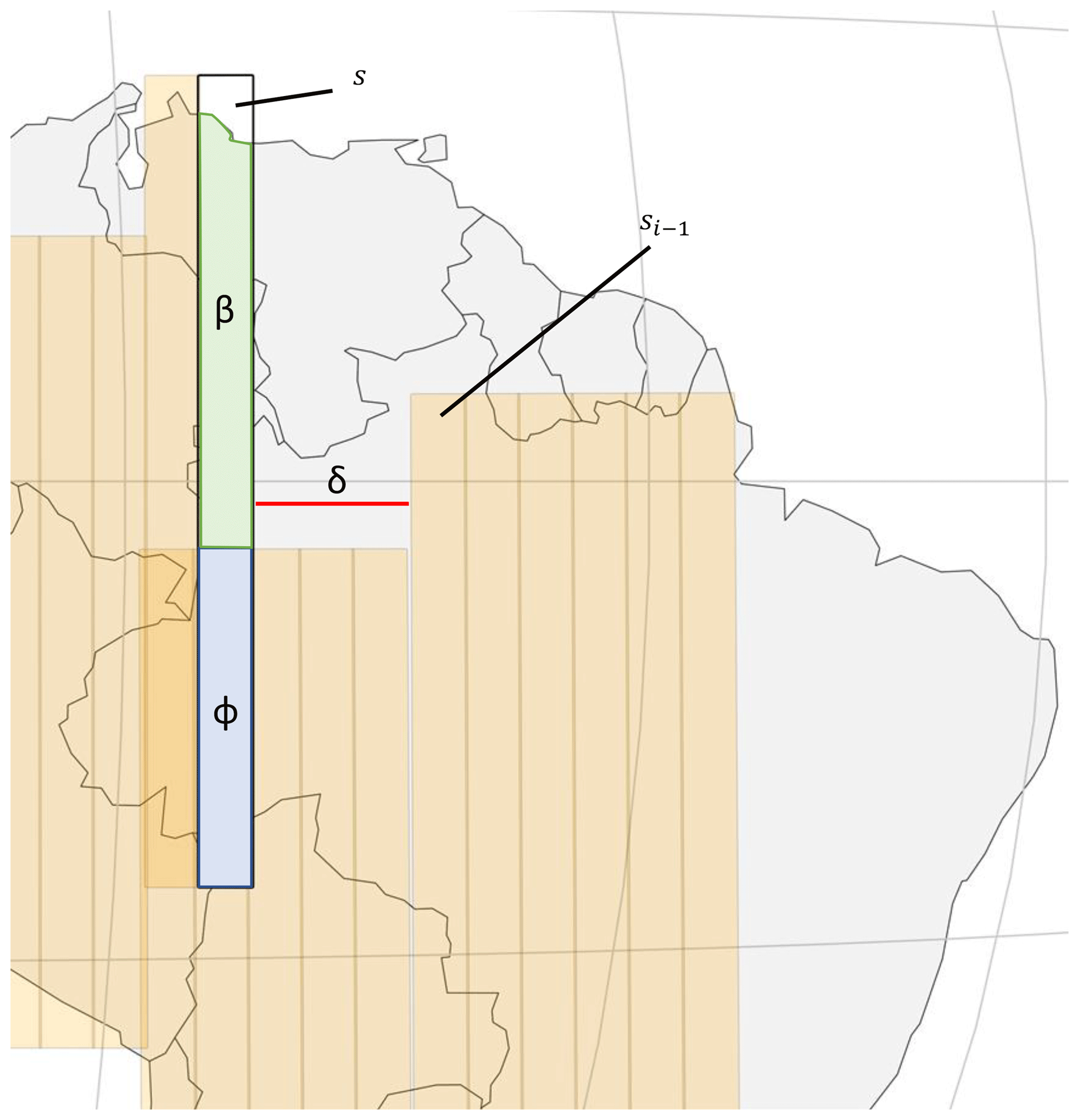
Figure 2 A diagram explaining the objective function, c(s,t), used in the IO routine. The block labeled s_i−1 is the last selected block and the block labeled s is the block for which c(s,t) is being calculated.

2 Background

GeoCarb will be hosted on a SES Government Solutions (http://www.ses-gs.com, last access: 24 May 2019) communications satellite in geostationary orbit at $\sim \mathrm{85}{}^{\circ }$ W. It will measure reflected sunlight in the O₂ band at 0.76 µm to measure total column O₂, the weak and strong CO₂ bands at 1.61 and 2.06 µm to measure XCO₂, and the CH₄ band at 2.32 µm for measuring XCH₄ and XCO. The O₂ spectral band allows for determination of mixing ratios and the measurement of SIF, as well as additional information on aerosol and cloud contamination of retrievals. The baseline mission for GeoCarb aims to produce column-averaged mixing ratios of CO₂, CH₄, and CO with accuracy per sample of 0.7 % (≈2.7 ppm), 1 % (≈18 ppb), and 10 % (≈10 ppb), respectively (Polonsky et al., 2014). Geostationary orbit offers two main advantages over low Earth orbit (LEO). First, the signal-to-noise ratio (SNR) is proportional to the square root of the dwell time for detectors limited by photon shot noise, and geostationary orbits enable longer observation times, thereby increasing SNR. Second, due to the flexibility of the scanning mirrors, areas with high and uncertain anthropogenic emissions of CO₂, CH₄, and CO may be targeted with contiguous sampling, relatively small spatial footprints, and fine temporal resolution allowing for several observations per day on continental scales.

Figure 3 Comparing air mass factors in September (a) and June (b).

Figure 4 Comparing surface albedo during the autumn equinox (a) and the summer solstice (b).

We are presented with the problem of finding an optimized scanning strategy for the GeoCarb satellite instrument. The underlying abstract mathematical problem related to optimizing the scanning pattern is the geometric set cover problem (Hetland, 2014). Given a finite set of points in space and a collection of subsets of those points, the objective is to find a minimal set of subsets whose union covers all the points in the space. The classical method for finding a solution to the geometric set cover problem is to employ a greedy algorithm. Greedy algorithms incrementally choose optimal solutions based on the available information at a given time. In the context of the geometric set cover problem, the greedy algorithm incrementally selects subsets that cover the highest number of uncovered points until all points are covered by the chosen subsets. Modifying the greedy algorithm to optimize an objective function at each iteration is a common routine for finding geometric solutions to spatial problems with no known analytical solutions.

The task of determining the locations of new observation sites so that the total number of required sites to cover an area is minimal has been solved using IO algorithms (Rayner et al., 1996; Gloor et al., 2000; Patra and Maksyutov, 2002). Finding an optimized scanning strategy for GeoCarb is identical to an observation network optimization problem. Therefore, these IO algorithms were prospective candidates for application to GeoCarb. Our goal was to find a minimal covering set that translates to a scanning strategy that is operationally efficient and minimizes global measurement error for the GeoCarb instrument.

3 Methods

Translating the idea of the geometric set cover problem to GeoCarb's application, the collection of geometric subsets is 5 min east-to-west scan blocks. The points in space to be covered are the North American and South American landmasses between 50^∘ N and 50^∘ S since this contains the regions relevant to the six science hypotheses mentioned in the introduction. Measurement errors are influenced by parameters that vary in space and time such as clouds, air mass, and solar zenith angle. Predicting cloud formation and quantifying the effects of clouds on measurement errors are active areas of research. For simplicity and computational efficiency, a cloud-free atmosphere is assumed in the simple instrument model. Surface albedo is assumed to be constant within the span of a day. Due to time dependency, solutions are in the form of ordered sets where the scan blocks are ordered by time of execution. These solutions are referred to in this paper as scanning strategies. With the simplifying assumptions making the problem computationally tractable and minimizing scan coverage over the ocean, a candidate set of 135 scan blocks is proposed in Fig. 1. This is a much larger candidate set than those of the network optimization studies that utilized evolutionary algorithms (Rayner et al., 1996; Gloor et al., 2000). Therefore, the computationally efficient IO algorithm, which is a modified greedy algorithm, was implemented to select scan blocks that minimize our objective function at each increment in time.

Figure 5 The baseline strategy (a) compared to an algorithm-selected strategy (b).

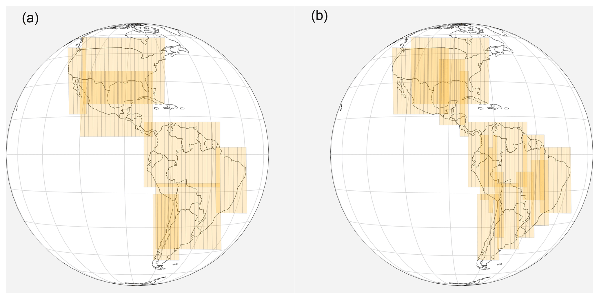
Figure 6 Violin plots show the effect of starting threshold on variance of errors: summer solstice (a) and autumn equinox (b).

Figure 7 Violin plots show the effect of starting threshold on error distribution medians: summer solstice (a) and autumn equinox (b).

3.1 Scan blocks

The scanning region is discretized in the east–west direction assuming that GeoCarb will process commands in terms of 5 min scan blocks. During the scan the instrument will step the slit from east to west within the scan block. Each slit observation is proposed to contain approximately 1000 individual soundings and is assumed to have a ∼9 s integration time. The scanning region is further discretized in the north–south direction by scan blocks separated by 5^∘ latitude increments. Potential scans that are primarily over the ocean are excluded since measurements over the ocean are not a priority for the GeoCarb mission. The scan blocks are also restricted to land between 50^∘ N and below 50^∘ S as a hard constraint due to larger sensor viewing zenith angles at the higher latitudes, though this area still includes all regions relevant to the six science hypotheses mentioned in the introduction. The resulting set of candidate scan blocks is shown in Fig. 1.

Figure 8 Global error distribution, baseline strategy (c, d), and algorithm-selected strategy (a, b).

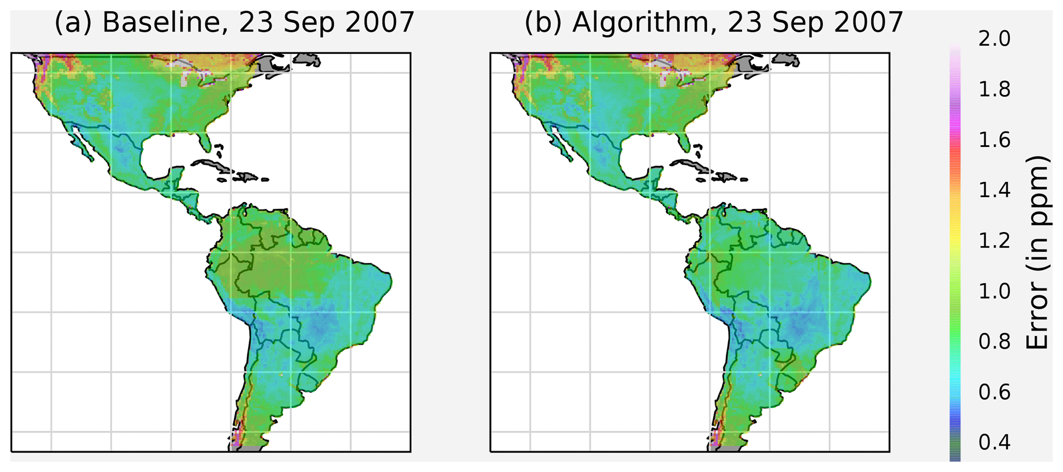
Figure 9 Comparison of the spatial distribution of XCO₂ errors of the baseline strategy (a) and the algorithm-selected strategy (b).

3.2 Science operations timeline

A goal of this study is to create a scanning strategy that views all landmasses of interest at least once within the time window of usable daylight. To determine what time of day to begin the scanning process, Macapá, Brazil, and Mexico City, Mexico, were chosen as geographic reference points to determine the beginning and ending time, respectively, of the usable daylight time frame. Macapá is located at (0, 50^∘ W) at the mouth of the Amazon River and being on the Equator gives us a consistent starting time relative to air mass factor (AF), a function of solar zenith angle (SZA) and the sensor viewing zenith angle (VZA), where AF $=\frac{\mathrm{1}}{\cos \left(\mathrm{SZA}\right)}+\frac{\mathrm{1}}{\cos \left(\mathrm{VZA}\right)}$. Located at 19.5^∘ N, 99.25^∘ W, Mexico City, Mexico, is an ideal reference point to determine when the window of usable daylight ended because it is longitudinally centered in the North American landmass while being close enough to the Equator for the calculated air mass factors to remain consistent through the winter months. The IO algorithm calculates the starting time when Macapá first exceeds a starting threshold for AF and the ending time when Mexico City drops below an ending threshold for AF to determine when the usable daylight time window is over. As a result of parameter exploration experiments described in Sect. 3.6, the suggested starting threshold is AF =2.6 for the summer solstice and AF =2.7 for the autumn equinox for minimum variance in predicted errors.

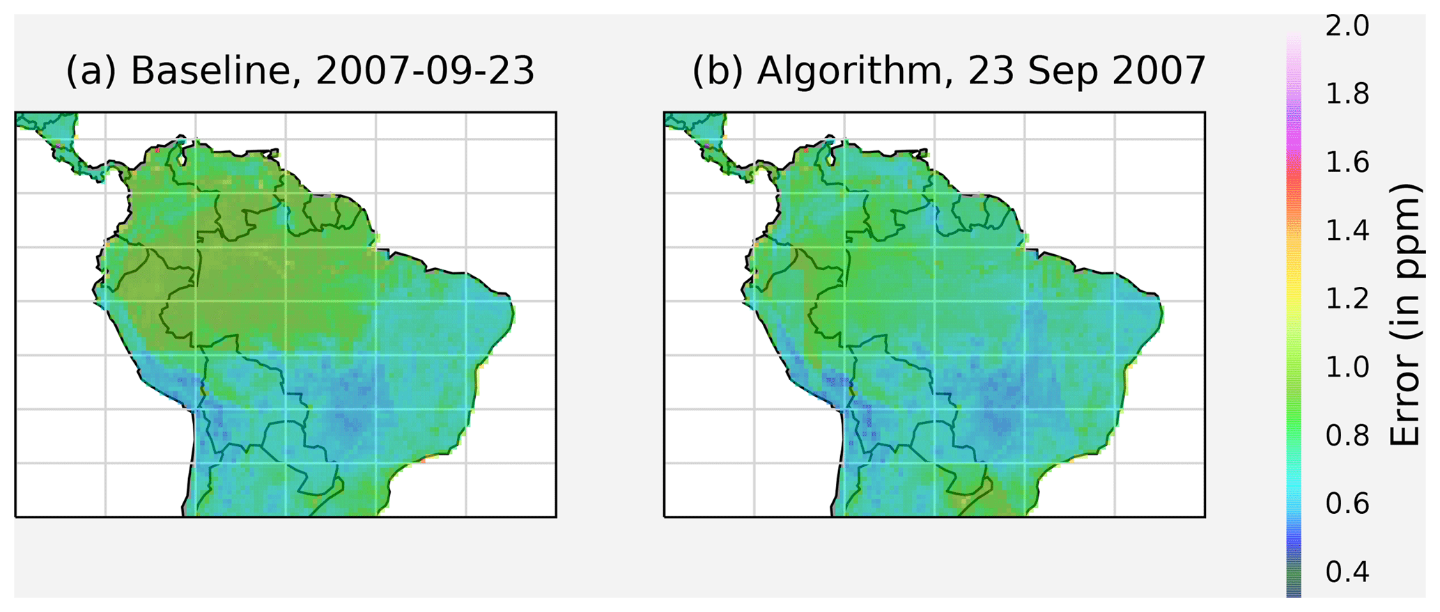
Figure 10 There is a significant improvement in predicted errors over the Amazon for the autumn equinox.

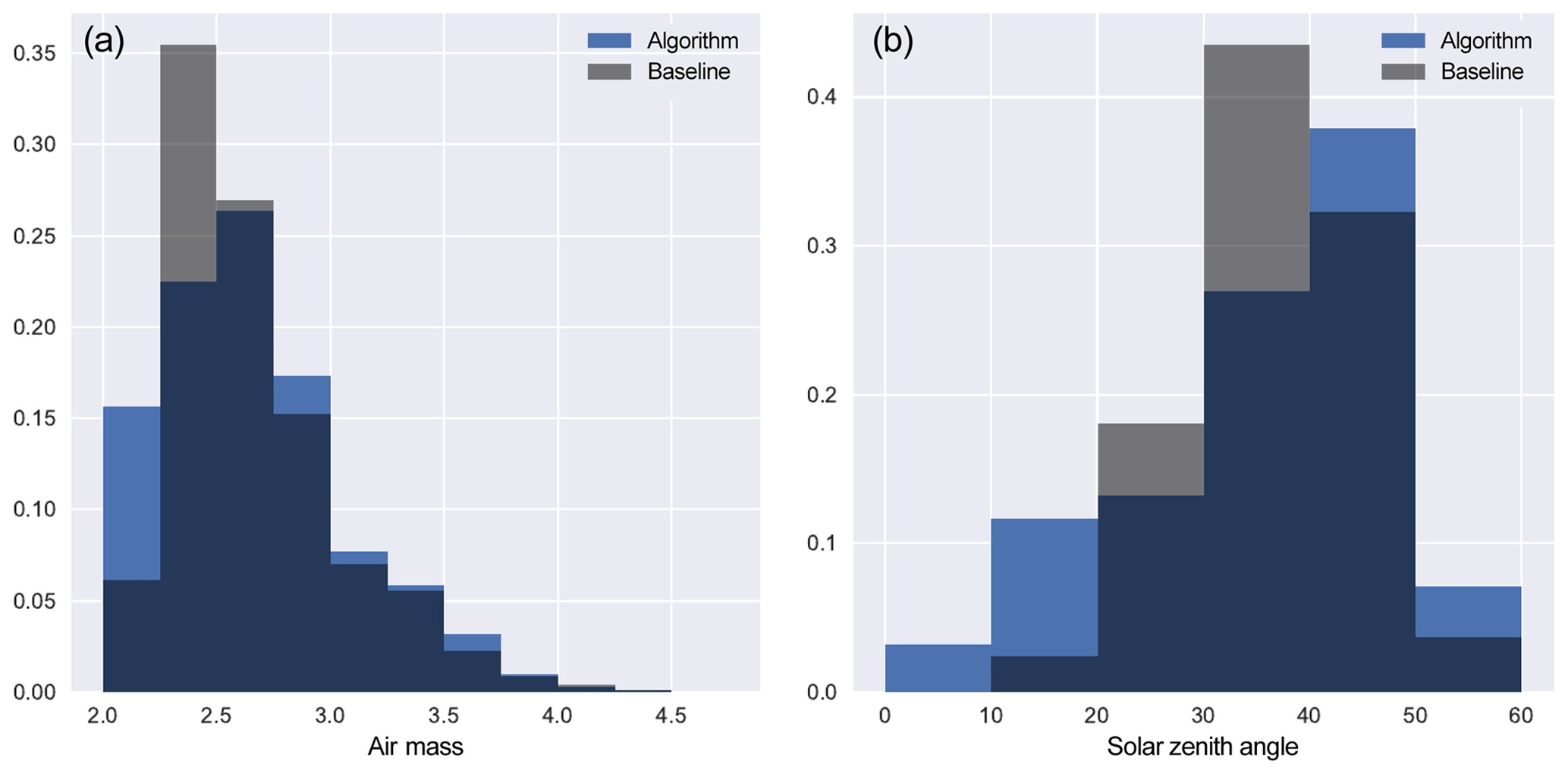
Figure 11 The histograms show that the algorithm selects more scan blocks with low AF (a) and low SZA (b) than the baseline strategy.

3.3 Uncertainty in retrieved gas concentrations

Errors in retrieved gases arise from a result of numerous different sources, including imperfect radiometric calibration, errors in differential absorption spectroscopy, variations in the instrument line shape, and others. For simplicity, we assume that the errors in retrieved gases arise from instrument noise as specified by a simple noise model arising from GeoCarb specific design parameters. The signal-to-noise ratio is then propagated through to uncertainty using a simple parameterization that was trained on retrieval results from simulated data.

The radiance observed by GeoCarb is an aggregate of insolation and atmospheric and land surface processes that absorb, reflect, and scatter photons. The impact of these processes is parameterized using a simple model, I, from Polonsky et al. (2014) that incorporates the effects of surface albedo and attenuation by aerosols over the sun–Earth–satellite path described by SZA and VZA:

$$\begin{array}{}\text{(1)}& {\displaystyle }I=F_{\mathrm{sun}}\mathit{\alpha }\cos \left(\mathrm{SZA}\right)e^{-\mathrm{AF}\mathit{\tau }}\mathrm{nW}{\left({\mathrm{cm}}^{\mathrm{2}}\mathrm{sr}{\mathrm{cm}}^{-\mathrm{1}}\right)}^{-\mathrm{1}},\end{array}$$

where F_sun is the band-specific solar irradiance, α is the band-specific surface albedo, and τ is the optical depth (OD) of atmospheric scatterers (e.g., aerosols, water). A cloud-free atmosphere is assumed for this simple model, whereas in the operational environment, clouds play a major role in retrieval quality due to poorly understood 3-D scattering effects. As can be readily verified, larger zenith angles lead to reduced signal for constant scatterer OD, as does smaller surface albedo. Note that τ is a quantity with significant spatial and temporal variability, as aerosol concentrations are modified by atmospheric dynamics, emissions, and chemistry. Typical values of τ in successful retrievals for OCO-2 are less than 0.6 for nadir soundings near the Equator and decrease as AF increases. Similarly, surface albedo varies with land cover type on small spatial scales, and throughout the year with vegetation density. The OD term was set to τ=0.3 as it was previously found to be a reasonable estimate for a “clear” sky retrieval (Crisp et al., 2004; O'Dell et al., 2012).

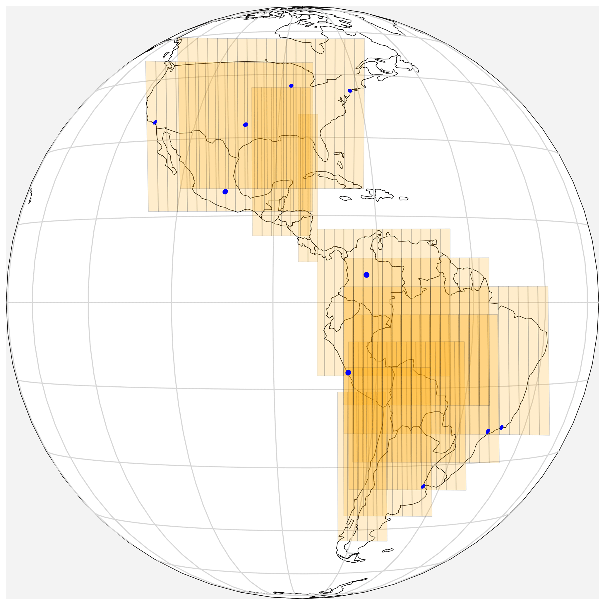
Figure 12 Scan blocks containing the 10 most populated cities are given higher weighting in city campaign mode.

Figure 13 Scaling factor for an observation point with minimum daily air mass factor, a=2.

An important indicator of observation quality is the signal-to-noise ratio (SNR). In the case of GeoCarb, the signal is modeled as I and the instrument noise equivalent spectral radiance model, N, as

$$\begin{array}{}\text{(2)}& {\displaystyle }N\left(I\right)=\sqrt{{N_{\mathrm{0}}}^{\mathrm{2}}+N_{\mathrm{1}}I}\mathrm{nW}{\left({\mathrm{cm}}^{\mathrm{2}}\mathrm{sr}{\mathrm{cm}}^{-\mathrm{1}}\right)}^{-\mathrm{1}},\end{array}$$

where N₀ and N₁ (nW(cm² sr cm⁻¹)⁻¹) are parameters that empirically capture the effects of the instrument design (e.g., telescope length, detector noise) on overall instrument noise (O'Dell et al., 2012). Constants that represent a signal-independent noise floor radiance, N₀=0.1296, and shot noise due to observed signal radiance, N₁=0.00175, specific to the weak CO₂ band (1.61 µm) are used in Eq. (2) to later calculate SNR. N₀ and N₁ are updated figures derived from the airborne trials with the Tropospheric Infrared Mapping Spectrometers (TIMS) by Lockheed Martin (Kumer et al., 2013), and later revised in Polonsky et al. (2014). The SNR is then defined as $\frac{I}{N}$.

In O'Brien et al. (2016), the authors fitted an empirical model to predict the posterior errors, σ, estimated by the L2 retrieval algorithm as a function of the measurement SNR. In their case, σ was derived from the L2 retrieval algorithm posterior covariance given by

$$\begin{array}{}\text{(3)}& {\displaystyle }\widehat{S}={\left(K^t{S}_{\mathit{ϵ}}^{-\mathrm{1}}K+S_a^{-\mathrm{1}}\right)}^{-\mathrm{1}},\end{array}$$

where S_ϵ is the covariance of the instrument noise, S_a is the covariance of the distribution about the prior state, and K is the Jacobian of the transformation from states to measurements. This uncertainty represents the impacts of the noise on the fitted spectra as well as nonlinearities in the radiative transfer model. It does not account for systematic errors that account from model deficiencies or instrument mischaracterization, which are beyond the scope of this work. O'Brien et al. (2016) found that the solid curves that best fit the posterior errors in the weak CO₂ band were of the form $\mathit{\sigma }=\frac{a}{\mathrm{1}+b{x}^c}$, where x is the SNR and $a,b,c$ are real constants. For CO₂, σ represents uncertainty in parts per million. For a SNR of x=0, the function takes its maximum value of a. Therefore, a represents the prior uncertainty. With large values of x, the constant c determines the rate of decay for σ. Setting a=14 ppm to express a conservative prior uncertainty on retrieved CO₂ and c=1, the resulting empirical model was

$$\begin{array}{}\text{(4)}& {\displaystyle }\mathit{\sigma }={\displaystyle \frac{\mathrm{14}}{\mathrm{1}+\left(\mathrm{0.0546}\right)x}}\mathrm{ppm}.\end{array}$$

The same model is used to connect SNR and uncertainty for evaluating scanning strategies later in this paper. For the purpose of our experiments, the distribution of σ is treated as the metric against which a particular scanning sequence is evaluated.

Figure 14 Compared to the baseline strategy (a), the overall performance of the algorithm-selected strategy (b) is not significantly degraded in the city campaign mode.

Figure 15 The algorithm-selected strategy (a) has approximately 2000 more usable observations than the baseline strategy (b) in the city campaign mode.

3.4 Objective function

Examining the definition of SNR, it is easy to see that SNR $\approx k\sqrt{I}$, where k is a constant. Therefore it is sufficient to focus on maximizing I. Maximizing I is equivalent to minimizing its multiplicative inverse, $\frac{\mathrm{1}}{I}$. Therefore, an objective function was defined that is approximately proportional to $\frac{\mathrm{1}}{I}$ on the parameters AF and surface albedo. In addition to minimizing SNR, two constraints were included in the objective function to prevent erratic scanning behavior. An overlap term, ϕ, was introduced to minimize repeated coverage of regions. A distance term, δ, was also included to prevent erratic scanning behavior. δ is the shortest linear distance from the boundary of the last selected scan block to a candidate scan block. The objective function, c, to be minimized is given by

$$\begin{array}{}\text{(5)}& \mathrm{c}(s,t)=\mathit{\psi }\left(\mathrm{1}+{\displaystyle \frac{\mathit{\varphi }+{\mathit{\delta }}^{\mathrm{2}}}{\mathit{\beta }}}\right),\end{array}$$

where s is the candidate scan block, t time, β area of uncovered landmass covered by the candidate scan block, ϕ area of overlapping coverage with selected blocks, ψ median of e^AFα⁻¹ over the entire area of the candidate scan block, and α the surface albedo of a point within a scan block. The terms ϕ, β, and δ are illustrated in Fig. 2 for clarity. The median of e^AFα⁻¹ is used because it is assumed that the distributions of air mass factor and surface albedo are non-Gaussian within the scan blocks due to the long viewing slit. The high variability of both parameters is described in Sect. 3.4.2.

3.4.1 Surface albedo

The MCD43C3 version 6 white-sky albedo MODIS band 6 data set (Schaaf and Wang, 2015) was utilized for obtaining surface albedo, α. The MODIS BRDF/Albedo product combines multiband, atmospherically corrected surface reflectance data from the MODIS and MISR instruments to fit a bidirectional reflectance distribution function (BRDF) in seven spectral bands at a 1 km spatial resolution on a 16 d cycle (Lucht et al., 2000). The white-sky albedo measure is a bihemispherical reflectance obtained by integrating the BRDF over all viewing and irradiance directions. These albedo measures are purely properties of the surface; therefore they are compatible with any atmospheric specification to provide true surface albedo as an input to regional and global climate models. The native data were aggregated to the 0.5^∘ spatial resolution and interpolated in time to daily resolution.

Table 1 This table shows for a sample of daily minimum AFs the distance relationship between the daily minimum AF of an observed point, a, and the scaling factor threshold, c, used in the modified objective function (Eq. 7).

3.4.2 Seasonal variation in parameters

Since AF is affected by the sun's position and albedo is affected by the density of vegetation, there are large seasonal variations in both of these variables, shown in Figs. 3 and 4. However, there is little to no variation between day-to-day comparisons of these variables. It suffices then, and gives an added advantage of being computationally efficient, to calculate separate scanning strategies for each month rather than day.

3.5 Optimization algorithms

The time dependency of the scanning strategy requires the solutions to be represented as ordered scan blocks of the discretized candidate set described in Sect. 3.1 and shown in Fig. 1. Therefore, the sum of permutations ${\sum }_{k=\mathrm{1}}^{\mathrm{135}}\frac{\mathrm{135}\mathrm{!}}{(\mathrm{135}-k)\mathrm{!}}$ gives approximately 7×10²³⁰ possible solutions. Since it is computationally intractable to evaluate all possible solutions, a greedy heuristic algorithm was employed to find a minimal covering set as a lower-bound estimate for the size of a solution set. The greedy algorithm was then modified to an incremental optimization (IO) algorithm to find a scanning strategy optimizing for SNR.

3.5.1 Greedy algorithm

Viewing the North American and South American landmasses as a uniform space to be covered without considering any additional constraints, the problem is a geometric set cover problem where the goal is to find a minimal size covering set that we will call optimal. It is well-known that there are no known analytical solutions to the set cover problem, as it is one of Karp's 21 NP-complete problems, and the optimization version is NP-hard (Karp, 1972). However, there exists a heuristic method for finding a solution called the greedy algorithm that selects the cover with the largest intersection with the uncovered space recursively until the space is covered (Hetland, 2014). The pseudo-code of the greedy routine is shown in Algorithm 1. The greedy algorithm is computationally efficient, but it is difficult to verify that the solution it finds is the optimal solution. The greedy algorithm is suitable for the purpose of finding the smallest size scanning strategy because it reduces the set of candidate blocks at each iteration by removing the selected scan blocks to ensure that there are no repeated scan blocks in a solution. Running the greedy heuristic with no objective function shows that the area of interest can be covered using 83 scan blocks. Therefore, this was taken as the lower bound of covering set size.

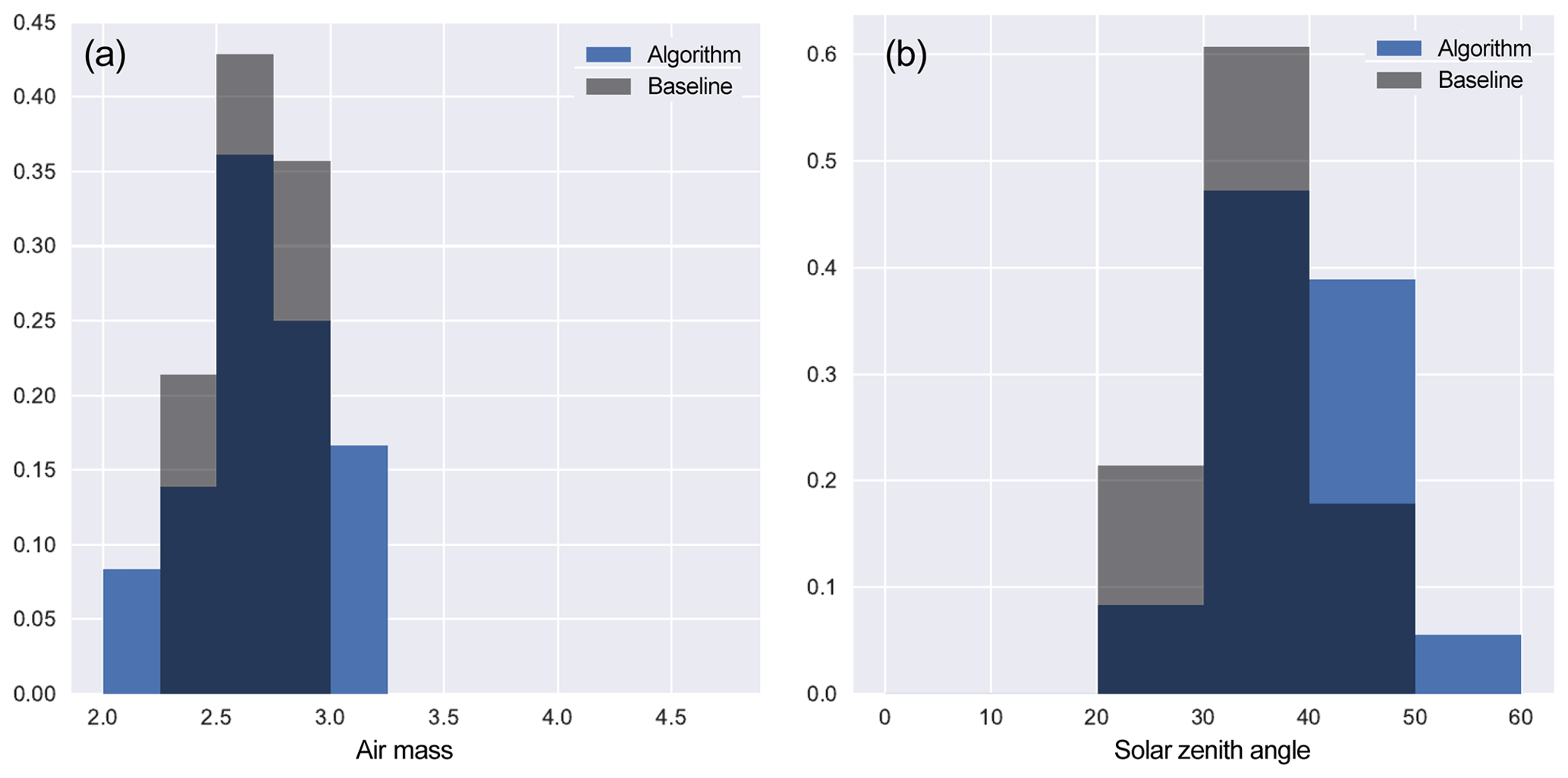
Figure 16 In the city campaign mode, the histograms show that the algorithm-selected strategy has more observations with low AF (a), but the baseline strategy's observations have lower SZA (b).

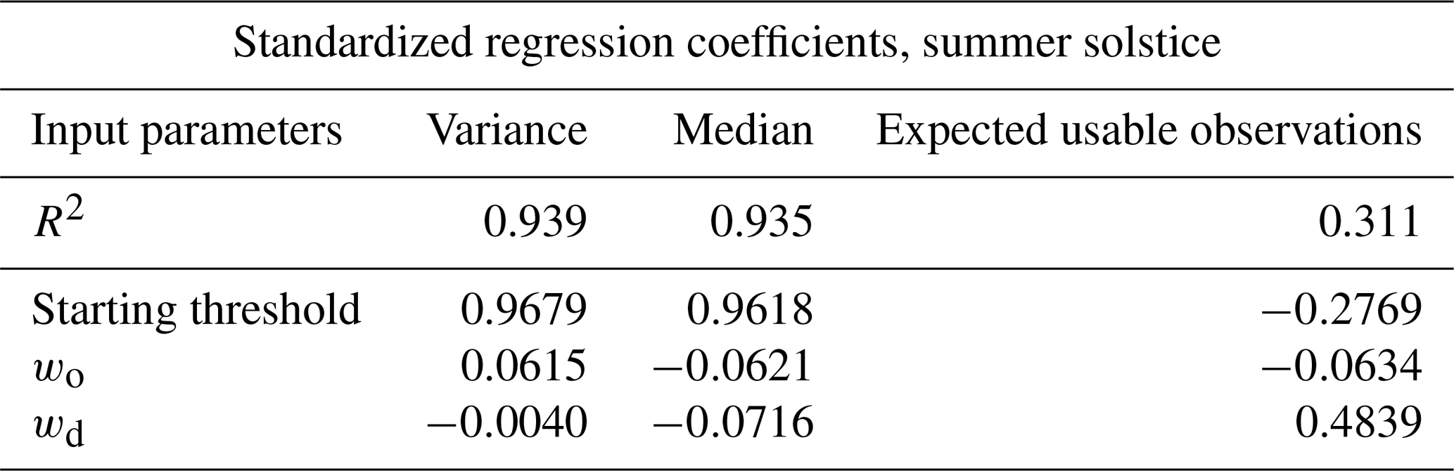
Table 2 The SRCs show that the variance and median of global error distributions are sensitive to starting AF thresholds.

3.5.2 Incremental optimization

The greedy algorithm was modified to select the scan block that minimizes the objective function at each iteration to satisfy operational constraints. Presented in Patra and Maksyutov (2002), this modification to the greedy algorithm is called an incremental optimization (IO) algorithm because its goal is to minimize the objective function at each increment of time to find the global optimum. Like the greedy algorithm, IO has the advantage of being computationally inexpensive. However, it may find local optima only and produce sub-optimal solutions depending on the nature of the problem. Usually to avoid this issue, small perturbations are introduced at each increment, such as is done in evolutionary algorithms (e.g., simulated annealing and genetic algorithm). It has been shown that IO yields results that are nearly as good as evolutionary algorithms while using a fraction of the computational power (Nickless et al., 2018).

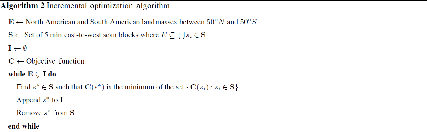
For GeoCarb's application, we were looking at the global distribution of errors, σ, and therefore were not concerned about local optima. An additional constraint was added that required the algorithm to cover South America before switching to North America to further prevent erratic scanning behavior. The pseudo-code of the IO algorithm is shown in Algorithm 2.

Table 3 The SRCs show that the median of global error distributions is sensitive to starting AF thresholds. The low R² value for variance indicates that there may be a nonlinear relationship between variance and starting AF threshold. Figure 6 shows that this is the case.

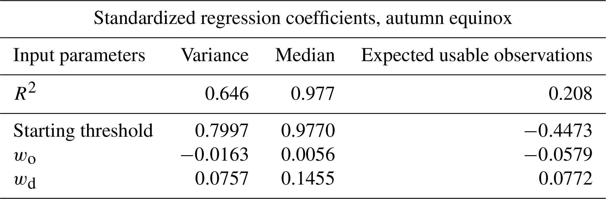
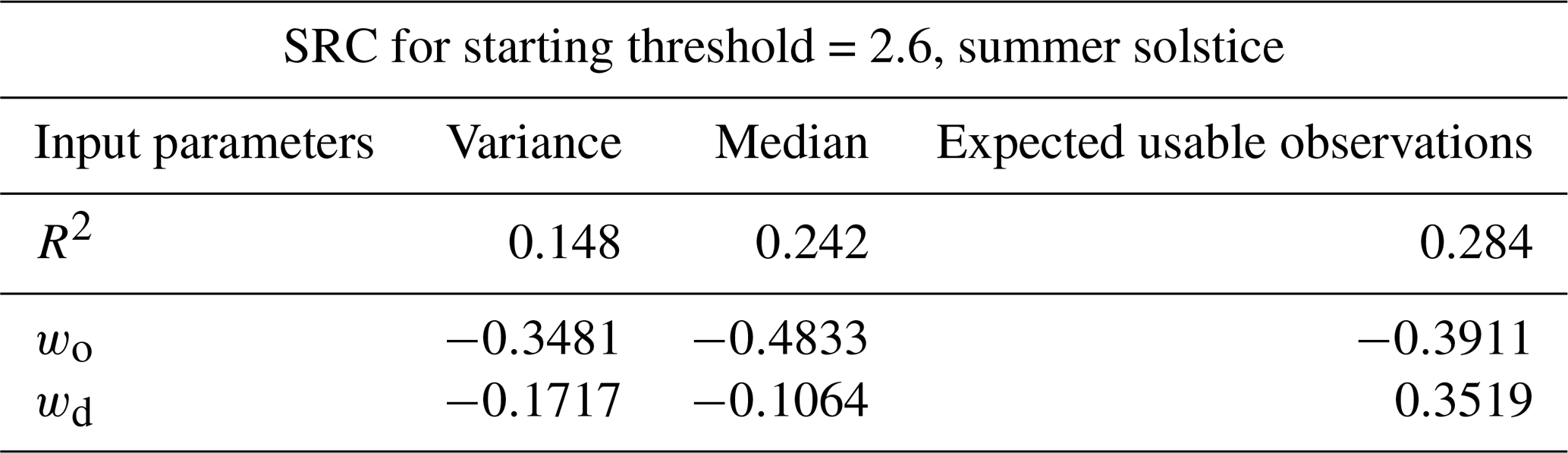
Table 4 The SRCs show that the median and variance of global error distributions are not sensitive to different weighting of the distance and overlap terms. R²<0.7 usually signifies insensitivity to independent variables.

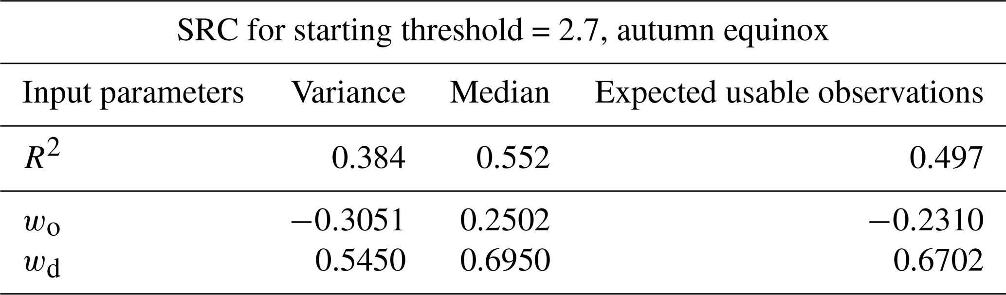
Table 5 The SRCs show that the median and variance of global error distributions are not sensitive to different weighting of the distance and overlap terms. R²<0.7 usually signifies insensitivity to independent variables.

3.6 Parameter exploration

The IO algorithm calculates a scanning start time from a specified starting AF threshold, described in Sect. 3.2, but it was unknown what overall effect the AF threshold had on the overall performance of the resulting scanning strategy. In the objective function (Eq. 5), the overlap and distance terms had equal weighting and different weightings were tested to understand their effects as well. A Monte Carlo experiment was performed to determine the distribution of sample error statistics across a range of possible starting AF thresholds and weights for overlap and distance. The effects of different weightings of the distance and overlap terms on the global distribution of errors were investigated specifically by adding (w_o,w_d) constant weight terms to Eq. (5) as new input parameters, resulting in

$$\begin{array}{}\text{(6)}& \mathrm{c}(s,t,w_{\mathrm{o}},w_{\mathrm{d}})=\mathit{\psi }\left(\mathrm{1}+{\displaystyle \frac{w_{\mathrm{o}}\mathit{\varphi }+w_{\mathrm{d}}{\mathit{\delta }}^{\mathrm{2}}}{\mathit{\beta }}}\right).\end{array}$$

Applying Eq. (6) to the algorithm gives the operator three inputs to specify, w_o, w_d, and the starting AF threshold. For both w_o and w_d, 1000 weights were randomly sampled from a uniform distribution between 0 and 10. This process was repeated for the summer solstice and autumn equinox for starting AF thresholds starting from 2.5 increasing by 0.1 to 3.5 for a total of 22 000 experiments. For these experiments, the contiguous landmasses of North and South America were scanned with equal importance. The minimum variance of predicted errors with respect to starting AF threshold occurred at 2.6 for the summer solstice and 2.7 for the autumn equinox, shown in Fig. 6. Both distributions of median and variance of errors averaged a 0.01 ppm spread over all values of w_o and w_d tested. Therefore, it was concluded that the effects of different weightings of the distance and overlap terms were negligible on the overall aggregate error, and weighting terms were excluded from the objective function. A sensitivity analysis was also performed to quantify the effects of these results and can be found in Appendix A.

3.7 Evaluating the optimized scanning strategy

For evaluating the performance of an algorithm-selected scanning strategy, the empirical distributions of error, σ (Eq. 4), were compared between the optimized strategy and a baseline scanning strategy proposed in Moore et al. (2018). An example of the two strategies is shown in Fig. 5. The baseline strategy tracks the sun's path from east to west and covers the entire area of interest in five coherent regions in the order of tropical South America east, tropical South America west, temperate South America, tropical North America, and temperate North America. The same scanning start times used by the IO algorithm are used for evaluating the performance of the baseline strategy. The times calculated by the algorithm, based on a starting AF threshold supplied by the user, were 12:30 UTC for the autumn equinox with a starting AF threshold of 2.6 and 13:15 UTC for the summer solstice with a starting AF threshold of 2.7.

In practice, a post-processing filter (PPF) is applied to retrieved satellite data and the data are marked with a quality flag to notify the end user of its overall usefulness. For this study, a threshold of 100 on the SNR is used as our PPF to determine a “usable” sounding. This threshold limits the predicted error to a maximum of ∼ 2 ppm, (Eq. 4), and is within the accuracy per sample performance requirements laid out in Polonsky et al. (2014).

4 Experiment 1 – equal importance for all landmasses

In the first experiment, all contiguous landmasses of North and South America were scanned with equal importance. Based on the parameter exploration results, simulations were performed for the summer solstice with a starting AF threshold of 2.6 and the autumn equinox with a starting AF threshold of 2.7 (Nivitanont, 2019a, b). The algorithm-selected scanning strategies consistently matched or exceeded the performance of the baseline scanning pattern, shown in Figs. 8 and 9. The region where the most significant improvement is seen is in the Amazon during the autumn equinox; refer to Fig. 10. After applying the PPF to the simulation results, it was clear that the greatest performance increase from the baseline strategy was in usable soundings. During the summer solstice, the algorithm-selected strategy yielded ∼3.79 million usable soundings versus ∼3.02 million usable soundings from the baseline strategy. During the autumn equinox, the algorithm-selected strategy yielded ∼4.31 million usable soundings versus ∼3.04 million usable soundings from the baseline.

Part of the increase in usable soundings can be attributed to the optimized strategy following the coastline better, which results in fewer scans over the ocean and more overlapping scans; refer to Fig. 5. However, the comparison of SZA and AF between the baseline and algorithm-chosen strategy shows that the algorithm also selects more scan blocks with low SZA and low AF; refer to Fig. 11. It is important to note that these figures are results from simulations performed in the cloud-free environment of the model. Realistically, there is a high probability that parts of the scanning slit will include cloudy scenes. We expect the yield of usable soundings to be significantly lower during operations, but those effects will be seen similarly in both the baseline and optimized strategies.

5 Experiment 2 – city campaign

A major advantage of having a geostationary platform is the flexibility to scan areas of high interest at times of optimal observing conditions. In this section, a “temporary campaign” mode is demonstrated where GeoCarb observes the 10 most populous cities in North and South America as areas of high interest, which are New York, Chicago, Los Angeles, Dallas–Fort Worth, Mexico City, Bogotá, São Paulo, Rio de Janeiro, Lima, and Buenos Aires. The demonstration is carried out for the autumn equinox with a starting AF threshold of 2.7. The areas of interest are given higher weighting in the algorithm through a modified version of Eq. (5). The performance of the resulting optimized strategies is compared to the baseline strategy, both globally and for the 10 cities of interest.

5.1 Modified objective function

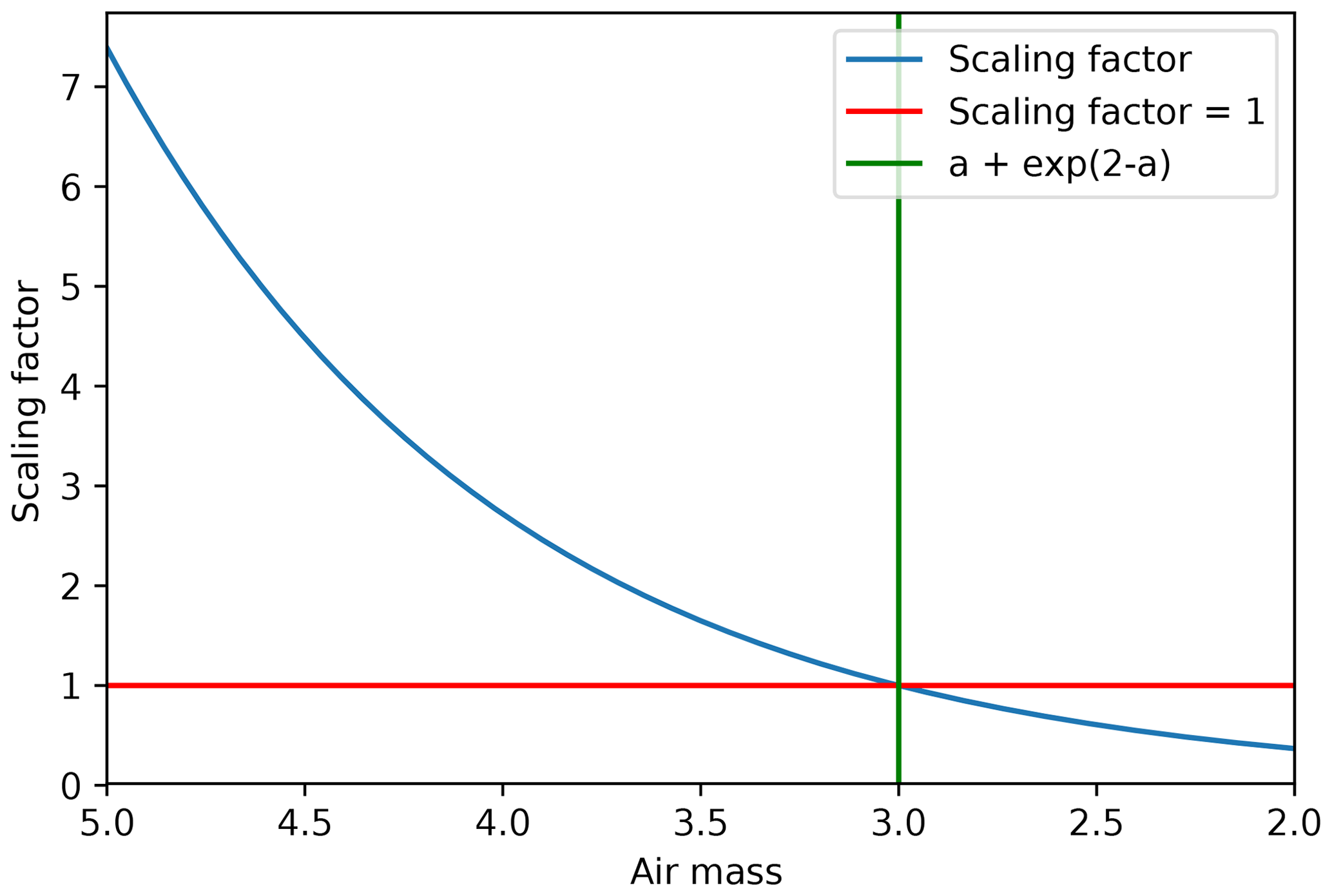
To give these areas of interest a higher weight, a time-dependent scaling factor was added to the term ψ in the objective function (Eq. 5) for scan blocks containing these cities; refer to Fig. 12. The scaling factor is defined as, e^b−c, where b is the AF of a point with respect to time and $c=a+e^{\mathrm{2}-a}$, where a is the daily minimum AF of the point. The term c acts as a threshold for the selection of the scanning block. While b is greater than c, the scaling factor penalizes the objective function by giving it a larger value, which tells the algorithm to wait on selecting the block until it is reasonably close to its minimum AF. Once b becomes less than c, the scaling factor scales down the value of the objective function to make the algorithm select the scan block as soon as possible. Figure 13 shows the scaling factor for a point with a minimum daily AF of 2. Table 1 shows the relationship between minimum daily AF and the scaling factor threshold for a sample of minimum AFs. The modified objective function is

$$\begin{array}{}\text{(7)}& c(s,t)=\stackrel{\mathrm{̃}}{\mathit{\psi }}\left(\mathrm{1}+{\displaystyle \frac{\mathit{\varphi }+{\mathit{\delta }}^{\mathrm{2}}}{\mathit{\beta }}}\right),\end{array}$$

where $\stackrel{\mathrm{̃}}{\mathit{\psi }}$ is the median of $e^{b-c}{e}^{\mathrm{AF}}{\mathit{\alpha }}^{-\mathrm{1}}$ over the entire area of a candidate scan block containing a city of interest.

5.2 Predicted errors

The addition of the scaling factor only affects the candidate scan blocks that contain a city of interest. Hence, there should be no significant degradation in the overall performance of the optimized scanning strategy. Figure 14 shows that there is still a significant increase in usable soundings, ∼3.97 million versus ∼3.03 million globally.

Looking at only observations over the 10 cities, the optimized scanning strategy shows an increase of ∼2000 usable soundings over the baseline strategy; refer to Fig. 15. Shown in Fig. 16, the baseline strategy's city observations have a higher concentration of low-SZA soundings, but the optimized strategy's city observations have a higher concentration of low-AF soundings.

6 Conclusions

We illustrate an efficient, offline technique that creates a geostationary scanning strategy that minimizes overall predicted measurement error. Applied in a simplified instrument model of GeoCarb, the IO routine gives us an optimized scanning strategy that performs better than the baseline scanning strategy relative to the global distribution of error and number of usable soundings. In Sect. 4, we showed that the incremental optimization of SNR with respect to the stationary physical processes, AF, and albedo results in an overall performance increase with the region of greatest performance increase seen in the Amazon (Fig. 9). We have also shown in Sect. 5 that the IO routine can be easily modified for a temporary campaign mode that focuses on the 10 most populated cities of North and South America. Other examples of possible scenarios for temporary campaigns are wildfires, droughts, and volcanic eruptions.

At the moment, our model does not take into account the effect of clouds on retrieval quality. It is known that clouds play a significant role in scattering effects and influences τ in the calculation of radiance (Eq. 1), but quantifying these effects is an active area of research. In a case study including clouds and aerosols in the atmosphere performed by Polonsky et al. (2014), the authors found that the number of usable soundings passing their post-processing filter (PPF) of aerosol optical depth (AOD) <0.1 was between 8.1 % and 20 % of total simulated soundings. We believe that an AOD threshold of 0.1 is too strict for the clear-sky atmosphere used in our simulations; therefore the threshold was relaxed to 0.3 to capture a conservative estimate of usable soundings as previously performed by O'Dell et al. (2012) and Rayner et al. (2014). O'Dell et al. (2012) found that 22 % of their simulated observations were classified correctly as clear when they used an AOD threshold of 0.3. Because we set τ=0.3 in our calculation of radiance (Eq. 1), our estimate is that the true number of usable soundings will be around 20 % of our simulated usable soundings in Sect. 4. Going forward, the incorporation of cloud products from CALIPSO will be investigated to better simulate operational conditions and produce more robust estimates of usable soundings.

The SNR-optimized scanning strategy outperforms the proposed strategy for the GeoCarb scientific observation plan. An empirical model that calculates predicted CO₂ retrieval uncertainty, σ, as a function of SNR was used to evaluate the performance of algorithm-selected strategies. The optimized scanning strategies consistently matched or exceeded the predicted performance of the proposed scanning strategy pattern with respect to aggregate distribution of σ. When a simple post-processing filter (PPF) of SNR >100 was applied to determine what constituted a usable sounding, the optimized strategies yielded a ∼18 % increase in usable soundings during the summer and a ∼41 % increase during the autumn over the proposed scanning strategy.

Appendix A: Sensitivity analysis

To quantify the algorithm's sensitivity to input parameters, the method of standardized regression coefficients (SRCs) was utilized (Helton et al., 2006). SRCs are the regression coefficients of a linear model fitted to the standardized dependent variable, $Y_Z=\frac{Y-\overline{Y}}{{\mathit{\sigma }}_Y}$, using standardized independent variables, $X_Z=\frac{X-\overline{X}}{{\mathit{\sigma }}_X}$. The dependent variable in this case is the predicted error and the independent variables are w_o, w_d, and the starting AF threshold. The standardization of variables allows for measuring the effect of the input parameters without their dependency on units (i.e., parts per million). The coefficient of determination, R², of the SRC model tells us how much of the variability in the sample statistics is explained by the SRC model. R² is defined as the modeled sum of squares (MSS) divided by the total sum of squares (TSS), where

$$\begin{array}{ll}{\displaystyle }\mathrm{MSS}& {\displaystyle }=\sum _{i=\mathrm{1}}^n{\left({\widehat{Y}}_i-\overline{Y}\right)}^{\mathrm{2}}\\ {\displaystyle }\mathrm{TSS}& {\displaystyle }=\sum _{i=\mathrm{1}}^n{\left(Y_i-\overline{Y}\right)}^{\mathrm{2}}\\ {\displaystyle }{R}^{\mathrm{2}}& {\displaystyle }={\displaystyle \frac{\mathrm{MSS}}{\mathrm{TSS}}},\end{array}$$

and $\widehat{Y}$ is model-predicted values, $\overline{Y}$ mean error, Y observed values, and n number of observations. The method of SRC was chosen for the sensitivity analysis by convenience of readily available simulation data from the parameter exploration experiment.

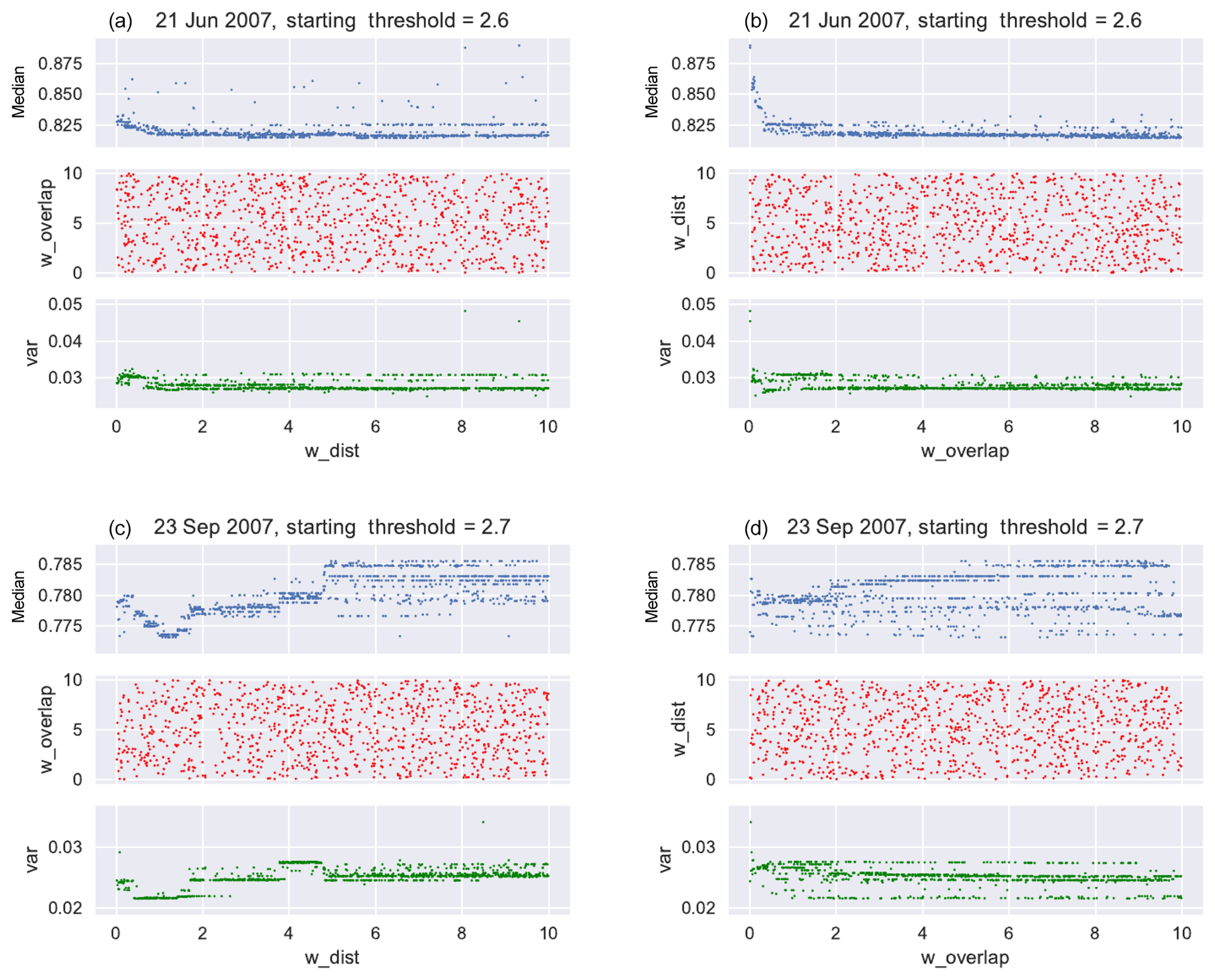
Figure A1 Scatter plots do not indicate a nonlinear relationship between weights and sample statistics. w_o and w_d are indicated as w_dist and w_overlap on the x axis.

The SRCs show that both the median and variance of the global error are found to be sensitive to starting AF thresholds as seen in Figs. 6 and 7 and Tables 2 and 3. This sensitivity was expected considering that air mass factors depend on time and play a large role in the calculation of radiance (Eq. 1). The starting AF thresholds affect the scanning strategy as a whole by shifting the scanning time frame. Because SRCs determine the effect of the input parameters in the presence of others, the SRCs fitted to a linear model of predicted error with respect to w_o and w_d were also analyzed within the Monte Carlo samples of starting AF threshold equal to 2.7 for the autumn equinox and starting AF threshold equal to 2.6 for the summer solstice.

Within the specified starting AF threshold of 2.7 for the autumn equinox, moderate effects of the weights were found on the sample global error distribution. The values in Table 4 show that the SRC model explains approximately half of the variability in median of global error distributions, R²=0.552, and the parameter with the largest effect on the variance is the distance, δ. With respect to variance of global error distributions, the SRC model explains less than half of the variability with R²=0.384. Again, the parameter with the largest effect is the distance term.

Within the specified starting AF threshold of 2.6 for the summer solstice, the effects of the weights on the sample global error distribution are small. The SRC model explains around a quarter of the variability in median of global error distributions, R²=0.242, and ∼15 % of the variability with R²=0.148, shown in Table 5. The parameter with the largest effect is the overlap term for both variance and median of error distributions.

R² values less than 0.7 signify low sensitivity to the independent variables or a nonlinear relationship between the independent and dependent variables. Visual analysis of the scatter plots of the distributions of sample statistics versus weights (Fig. A1) does not imply a nonlinear relationship between the weights and sample statistics. It is important to note as well that the non-standardized sensitivity of predicted errors with respect to w_o,w_d, results in a spread of 0.01 ppm in the overall performance of an algorithm-selected scanning strategy. We conclude that the weighting terms contribute negligible effects to the algorithm's performance.