the Creative Commons Attribution 4.0 License.
the Creative Commons Attribution 4.0 License.
 | 20 Dec 2019
In-flight calibration and monitoring of the Tropospheric Monitoring Instrument (TROPOMI) short-wave infrared (SWIR) module
Richard M. van Hees
Paul J. J. Tol
Ilse Aben
Ruud W. M. Hoogeveen
During its first year in operation the short-wave infrared (SWIR) Tropospheric Monitoring Instrument (TROPOMI) was calibrated in-flight and its performance was monitored. In this paper we present the results of the in-flight calibration and the ongoing instrument monitoring. This includes the determination of the background signals, noise performance, instrument spectral response function (ISRF) stability, and stray-light stability. From these results, the number of incurred dead and bad pixels due to cosmic-ray impacts is determined. The light-path transmission is checked by monitoring internal lamp and diffuser stabilities. Due to its high sensitivity to Earth radiation on the eclipse side, the calibration strategy for the background (i.e. dark current and offset) monitoring was adjusted. Trends over the first full year of nominal operations reveal a very stable SWIR module. The number of newly incurred dead and bad pixels is less than 0.1 % over nearly a full year since the start of operations. Assuming linear degradation of various components, the SWIR module is expected to keep performing within expected parameters for the full operational lifetime.
- Article
(24390 KB) - Full-text XML
- BibTeX
- EndNote


The Sentinel-5 Precursor mission (better known as S5P; Veefkind et al., 2012), is the first mission within the scope of the European Union Copernicus programme1 which is dedicated to mapping and monitoring the chemical composition of the Earth's atmosphere. S5P is a precursor mission for the atmospheric composition Sentinel-5 missions, which produce the same global coverage as S5P. The Sentinel-5 missions are scheduled to launch in 2022 and beyond. The Tropospheric Monitoring Instrument (TROPOMI2) is the sole instrument onboard S5P. It consists of two modules: a ultraviolet, visible and near-infrared (UVN) module (Veefkind et al., 2012) and a SWIR module3 (Hoogeveen et al., 2013). The wavelength ranges include the spectral signatures of key trace gases that strongly influence climate and air quality. The SWIR module is aimed at measuring column densities of carbon monoxide (CO) and methane (CH4). Hoogeveen et al. (2013) presented the detector performance. TROPOMI produces daily global coverage column density maps of these gases using a swath of approximately 2600 km across track. Images are taken every 1.08 s, yielding spatial pixels of approximately 7×7 km2 at nadir. Note that since 16 August 2018 the resolution of TROPOMI has be improved; images are now taken every 0.8 s, yielding spatial pixels of approximately 7×5.5 km2 at nadir. The SWIR spectral range (2305–2385 nm) is sampled at 0.1 nm, and the spectral resolution is 0.22 nm.
With a total envisioned lifetime of 7 years, the mission will provide a unique insight into the chemical composition of our atmosphere. TROPOMI will be an essential tool to investigate both naturally and anthropogenically induced chemical variations at timescales from days to years.
S5P was launched on 13 October 2017, from Plesetsk, Russia, into an ascending sun-synchronous orbit with an Equator crossing time of 13:30 mean local solar time at an altitude of approximately 824 km. After launch, the first month was dedicated to outgassing and stabilization. TROPOMI was kept warm to prevent the detector (in particular the SWIR detector) from acting as a cold trap and, thus, to avoid contamination; the S5P cooler door was opened on 7 November 2017. In the following week, the SWIR detector and spectrometer cooled down to their operational temperatures of 140 and 202 K respectively.
Between the launch and 30 April 2018, the commissioning phase, also referred to as phase E1, was carried out with the aim of completing the calibration of the instrument, checking the data processing chain, and preparing for the nominal operations phase, referred to as phase E2. Nominal operations started on orbit number 2818. During nominal operations, it is necessary to monitor the instrument calibration derived on the ground. This is carried out using measurements from the eclipse side of each orbit. TROPOMI covers the entire planet Earth each day in 14.5 orbits. For the SWIR module, monitoring is performed for the background signal, the instrumental noise, the quantification of the pixel quality, validation/monitoring of the instrumental spectral response function (ISRF), and stray-light correction. Corrections are based on so-called calibration key data (CKD). The ISRF correction algorithm, the ground-based calibration, and the ISRF CKD derivation are reported in van Hees et al. (2018). All elements of the stray-light correction, including the CKD derivation, can be found in Tol et al. (2018). The CKD for the offset, dark-current, noise, and pixel quality were derived on the ground. Signals of the sun, as seen over the two diffusers, and signals of the internal lamps are monitored to quantify any transmission changes of the various components within the SWIR module.
In this paper we will report on the results of the commissioning phase, the monitoring during the first full year of nominal operations, and provide an outlook regarding the durability and future performance of the SWIR module. The outline of the paper is as follows: Section 2 details the calibration plan; Section 3 presents the results of the commissioning phase; Section 4 describes the monitoring results and trends of the first year of TROPOMI; and conclusions are given in Sect. 5.
2.1 Calibration plan
The calibration of SWIR is done primarily using data obtained during the ground-based calibration campaign (Kleipool et al., 2018). It is a key part of the calibration plan to monitor the quality of the results obtained from these ground-based calibrations over the lifetime of TROPOMI and update procedures and/or the CKD if necessary.
There are several types of measurements available for in-flight calibration:
-
spectral radiance (i.e. backscattered and/or thermal radiation from the Earth, available for both for the day- and night-side). This includes background measurements taken in the eclipse with an open folding mirror (FMM);
-
measurements with a closed FMM, looking into the onboard calibration unit (CU);
-
spectral irradiance (i.e. radiation from the sun).
The spectral irradiance signal passes over one of two diffusers to scale the signal to measurable levels. The first diffuser is used daily to measure the signal. The second diffuser is used weekly, thus enabling the detection and/or monitoring of degradation of the first diffuser.
When the FMM is closed, the SWIR module can be illuminated by several onboard calibration sources installed specifically for in-flight monitoring of calibration parameters. This is done by rotating the central diffuser carousel. In addition to the background measurements (i.e. all sources turned off), the following onboard illumination sources are relevant4 for the SWIR module:
-
the DLED, which is a dedicated “detector LED” emitting with a known smooth spectral profile at the SWIR wavelengths;
-
the WLS, which is a “white light source”;
-
the SLS, which is a “spectral line source” comprised of five dedicated diode lasers in the SWIR spectral band.
The DLED (detector LED) is placed in front of the detector behind the immersed grating, whereas the SLS and WLS are located in the calibration unit and, thus, follow almost the complete optical path. This is an important difference to distinguish the effects of the full optical path, or of the detector alone.
The five onboard tuneable distributed feedback lasers, or SLS, are unique to the SWIR module. These lasers are able to scan small parts of the wavelength range by changing the laser temperature using a thermoelectric cooler integrated into the laser housing. The range is about 70 detector pixels (∼7 nm), Due to operational constraints, the laser scan is carried out over 0.6 nm with a fixed diffuser (see van Hees et al., 2018 for more details on the capability of the SLS diffuser to be used in either fixed or oscillating mode.). The central wavelength of each laser has been selected to be able to sample different parts of the SWIR wavelength range. The signal of the SLS passes over a dedicated diffuser. This diffuser can be employed in oscillation mode to suppress speckles observed in the laser signal or in fixed mode. Due to the limited operational lifetime and excess heat produced by the oscillating diffuser, the calibration plan is to not oscillate the diffuser during nominal operations (van Hees et al., 2018). The location and light paths into the SWIR module of the onboard illumination sources are shown in Fig. 1. The DLED is located inside the SWIR module.
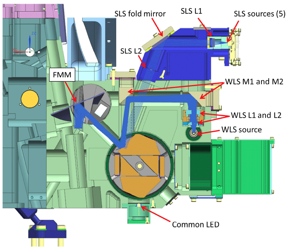
Figure 1Instrument layout indicating the location of the onboard illumination sources. The light paths of the SLS and WLS are shown using blue lines. The DLED is located within the SWIR module. The location of the CLED is shown. However, as it is not emitting any light at SWIR wavelengths, it is not used for SWIR calibration or monitoring. Figure courtesy of Airbus Defence and Space Netherlands and TNO.
Table 1 lists the parameters for which calibration parameters, the CKD, or monitoring data are derived. Measurements are taken in-flight to monitor whether the CKD can still be applied correctly during data processing. For calibration, we identify static, dynamic, and monitoring quantities. Static CKD are not dynamically updated in the processor following measurement results, whereas dynamic CKD are automatically updated. Static can be manually adjusted if warranted. Monitoring quantities are only monitored, but do not have a direct relation to CKD parameters. However, changes in these parameters will often initiate analysis regarding the applicability of the current calibration. Monitoring of all of these quantities is essential for the health monitoring of the SWIR module. Currently all CKD are static.
Table 1Calibration and monitoring data obtained in-flight.

a The Noise CKD is static. However, the in-flight noise of the detector is measured dynamically as input for the monitoring of the quality. Read noise was derived on the ground. b The quality map does not use direct measurements, but uses the dynamically measured dark current and in-flight noise. c The PRNU (pixel to pixel nonuniformity) stability is included in the comparison of the different light sources. d The ISRF is not used in the L1b data processing, but is used in the SWIR retrievals such as CO or CH4.
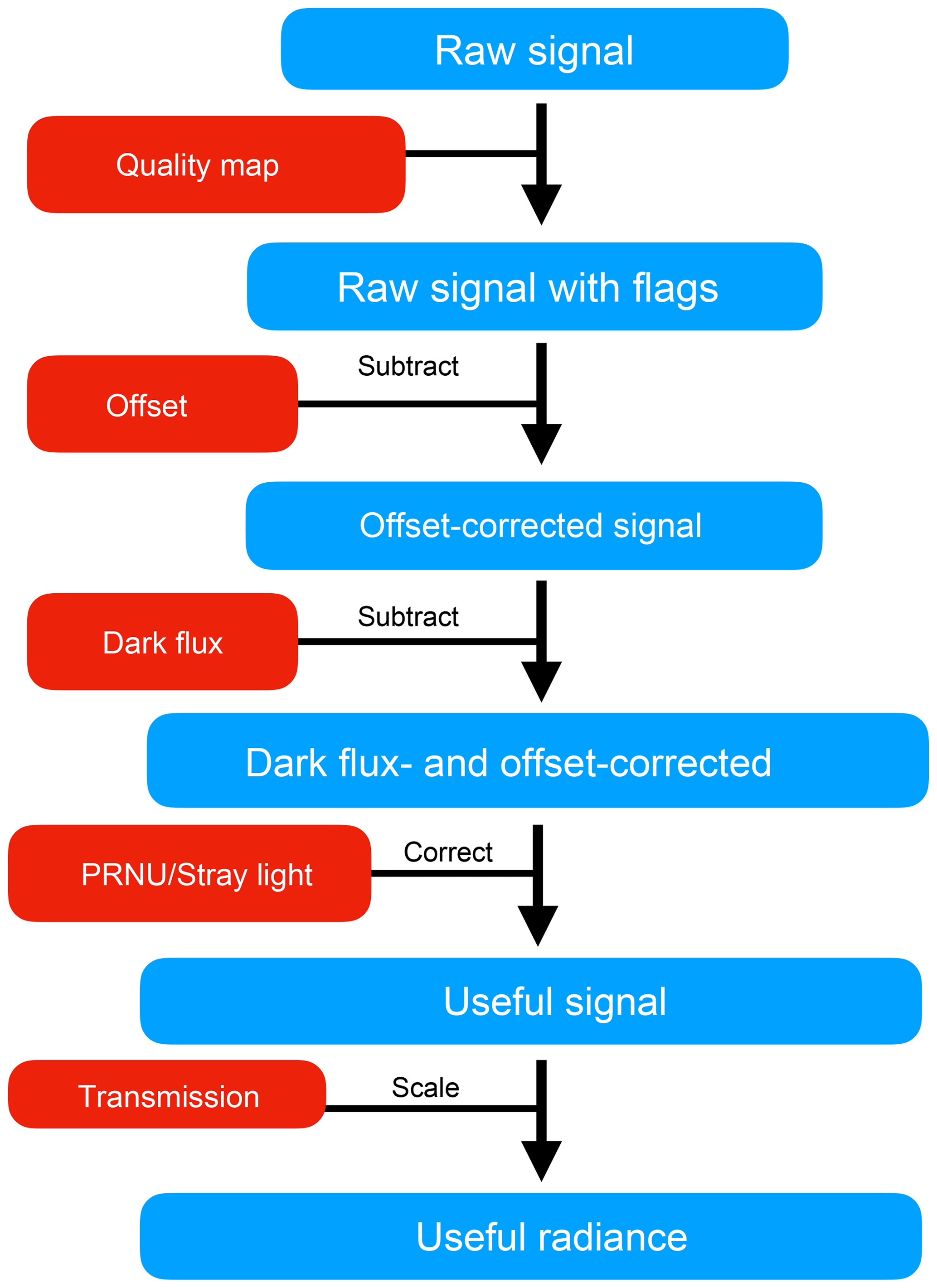
Figure 2Summary flow chart of the processing chain of a SWIR signal. This describes the processes that require monitoring in-flight. It assumes unit conversions are correctly carried out to produce useful radiance in spectral radiance units.
2.2 Processing chain
Data from TROPOMI SWIR are taken from a detector array consisting of 1000 pixels in the spectral dimension (columns) and 250 pixels in the spatial dimension (rows) of which 960 columns and 215 rows can be illuminated. Each pixel is read out individually through a CMOS read-out IC (Hoogeveen et al., 2007), but the exposure time is identical for all pixels in the detector. Exposure times during nominal operations range from 82 ms to typically 1080 ms. Shorter exposure times are used to avoid detector saturation in case of high-input light levels. For reference, to be used in the remainder of the paper, a pixel signal can be between 0 and 500 000 electrons, leading to electrical signals between 0.5 and 3.5 V, typically digitized with 12 000 binary units (BU). A raw TROPOMI-SWIR signal consists of three components: an offset, which is independent of exposure time; a dark signal, which is dependent on exposure time; and an outside signal. The outside signal can either be the Earth radiance, solar irradiance, or signal from the onboard lights; outside signal includes stray light. To accurately derive the useful signal (i.e. the outside signal), the offset and dark-current signals must be determined with high precision and subsequently subtracted from the raw signal. To calibrate the useful signal, the outside signal has to be corrected for several factors that influence the signal, such as the transmission (i.e. due degradation of components in the optical path, possibly resulting in light lost), pixel response nonuniformity (PRNU), and the influence of stray light. Stray light is defined as any outside signal that does not follow the intended path onto the detector and is thus not part of the useful signal. It may include ghosts, out of field stray light, out of (spectral) band stray light, or other forms. Stray-light correction for the SWIR module is extensively discussed in Tol et al. (2018). In-flight stray-light monitoring is discussed in Sect. 3.5.
Hoogeveen et al. (2013) mentions a few other effects that are observed in the SWIR detector. A small pixel-memory correction is applied when the exposure time is equal to the cycle time (i.e. 1080 or 800 ms). With faster detector readout, data are typically co-added, making the memory error smaller, and more difficult to correct for. Therefore, co-added data are not corrected for memory effects. Given the range of typical exposure times, nonlinearity of the detector was judged to be too small to justify a complex correction algorithm. The wavelength calibration is not specifically monitored, but follows from trace gas retrieval algorithms where small wavelength shifts are fitted within the procedure. The flow chart in Fig. 2 summarizes the full SWIR calibration process.
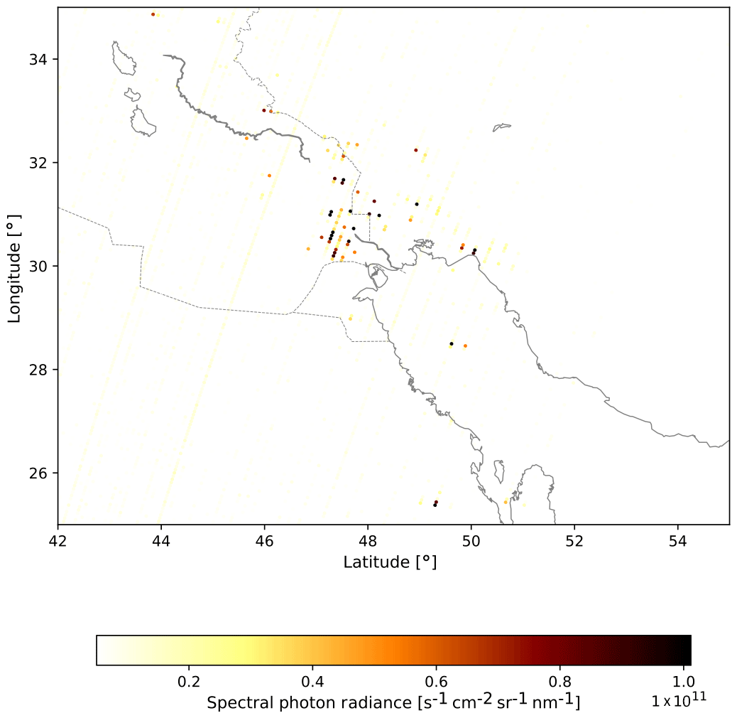
Figure 3Continuum radiance at 2314 nm on the eclipse side of the Earth around the Iraqi city of Basra. Any stripes in the figure are limitations of calibration and thermal stability at the time. Localized enhanced signals are clear indications of emission sources on Earth.
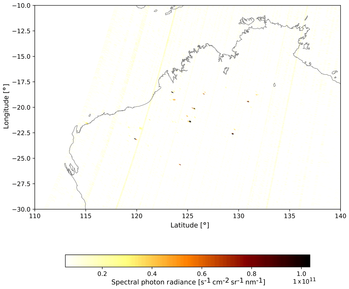
Figure 4Continuum radiance at 2314 nm on the eclipse side of the Earth for the north-western Australian outback. Any stripes in the figure are limitations of calibration and thermal stability at the time. Localized enhanced signals are clear indications of emission sources on the Earth.
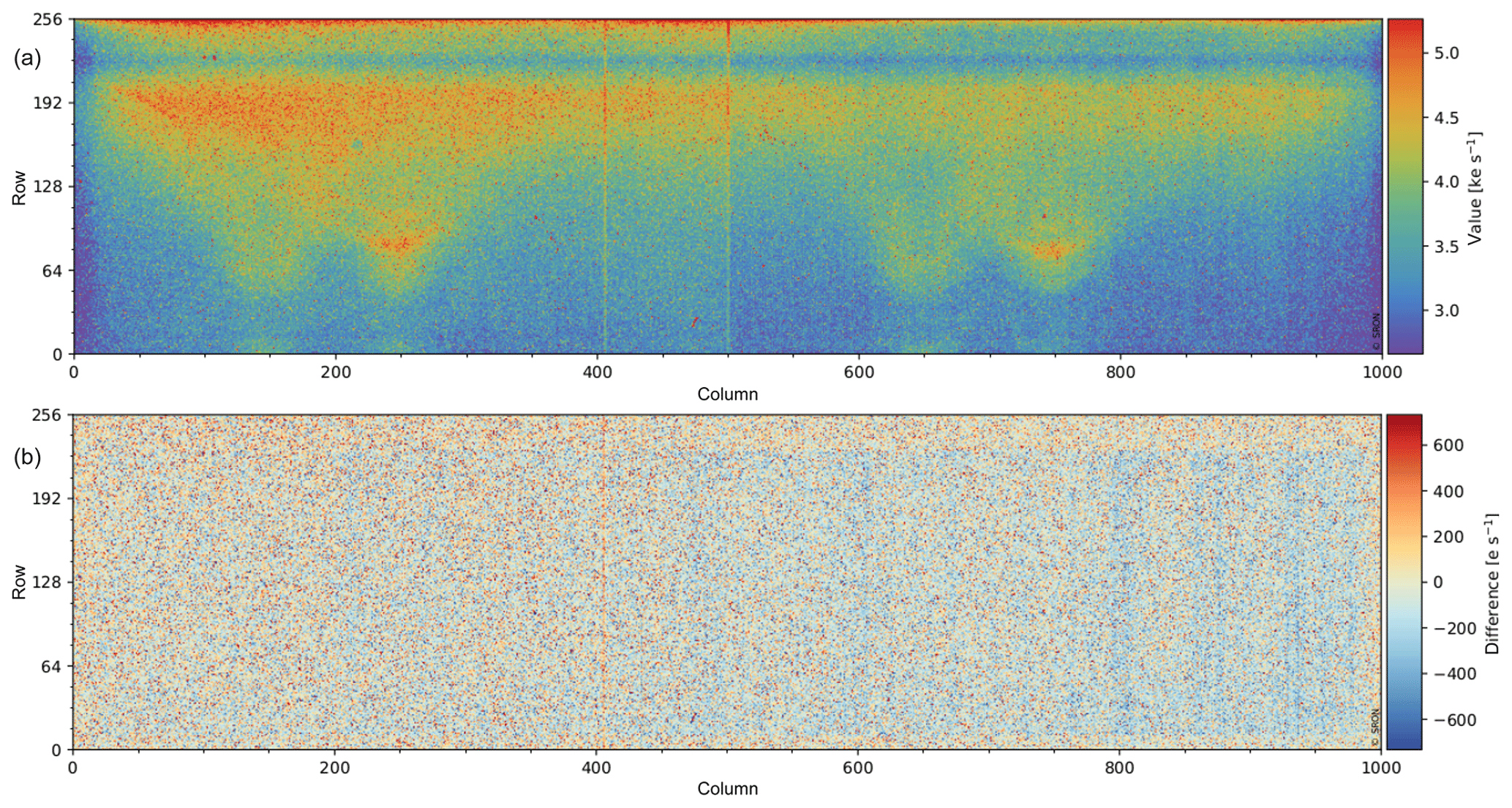
Figure 5The typical dark current obtained with the FMM open during the commissioning phase using data from orbits 990 to 1004 can be seen in panel (a). Data are plotted over the detector with the horizontal axis equivalent to the spectral direction and the vertical axis equivalent to the spatial swath. Panel (b) shows the result with the ground-based results subtracted.
3.1 Dark current and offset
3.1.1 Method
The value of the offset and dark-current corrections are determined from measurements on the eclipse side of the orbit (see Table 1). Measurements are carried out with identical instrument settings (exposure time and co-adding factor) as the radiance measurements on the solar illuminated side of the orbit. The exposure times range from 178 ms over the Equator to 538 ms over the poles. Before launch, it was assumed that the eclipse side of the Earth was dark and that the raw signal would be composed of only the offset and dark current5. A linear fit using measurements at a range of exposure times will yield the offset (signal at exposure time zero) and dark current (slope of the fit). In total, derivations are carried out every 15 orbits, using all background measurements within those 15 orbits.
3.1.2 Background with the FMM open
Figures 3 and 4 show the radiance of the SWIR continuum at 2314 nm on the eclipse side of the orbit around two regions: the northern part of the Persian Gulf and north-western Australia. Data were taken from orbits 430 and 433, measured during the “first light” campaign during November 2017. All exposure times were 216 ms.
In both Figs. 3 and 4, small regions and point sources are clearly visible with signals more than an order of magnitude higher than the background. Given the location, the sources are most likely the burning of excess natural gas at oil field installations (Basra) or natural wildfires (Australian outback). Inspection of other data yields many other emission sources over land including other bush fires and volcanic activity.
At larger spatial scales, thermal radiation of the Earth at night is detected by the SWIR module both over land and over oceans. Thermal radiation of the oceans appears brighter, presumably due to the inherently longer cooling times of water. However, even at high latitudes, radiances are clearly nonzero on the eclipse side of the orbit.
Figure 5 presents the dark current at the detector level using measurements with the FMM open. Figure 5a shows the results, whereas Fig. 5b shows the difference with the dark current derived from the ground-based calibration. Statistics of the results over the entire detector, i.e. the bi-weight median and spread6, are given in Table 2. The comparison reveals the following:
-
The overall structure of the dark current on the detector is reproduced (see Hoogeveen et al., 2013).
-
The median over the detector is somewhat lower (61 e s−1).
-
The difference in spreads is significant due to the amount of data used in obtaining the results.
-
Specific spectral features can be seen in the comparison with the ground-based calibration (Fig. 5 in the form of blue bands). The wavelengths correspond to deep absorption bands of water and methane in the atmosphere. No atmosphere was present during the ground-based reference measurements. The detector temperatures in-flight and on the ground were identical. Thus, absorption of the Earth's thermal radiation by water and methane occurs, causing this difference. These also do not extend to the top and bottom rows of the detector, which are covered.
-
Stronger differences are seen in columns 400 and 500. Column 500 is due to the edge of the analogue digital converter (ADC) areas. The difference in column 400 is unexplained.
Analysis of a range of measurements over 3 months also revealed differences with the ground-based calibration results which vary in time by approximately 20 e s−1. No trend was seen, but local changes in e.g. Earth's temperature field or weather can influence the results. These are partially mitigated by taking a bi-weight median over all available data, but this method cannot completely remove these effects.
The amount of dark current detected differs from the measured value reported in Hoogeveen et al. (2013). They present a median in the central area of 0.7 fA, equivalent to 4400 e s−1. This is likely attributed to the different thermal conditions of the set-up, as a significant part of the dark current is caused by the thermal emission of the spectrometer, which was absent in Hoogeveen et al. (2013).
The nonuniformity of the Earth's thermal radiation also introduces another significant bias. As most calibration measurements are taken near the warmer Equator, the measurements are not representative of the complete orbit that includes the polar regions.
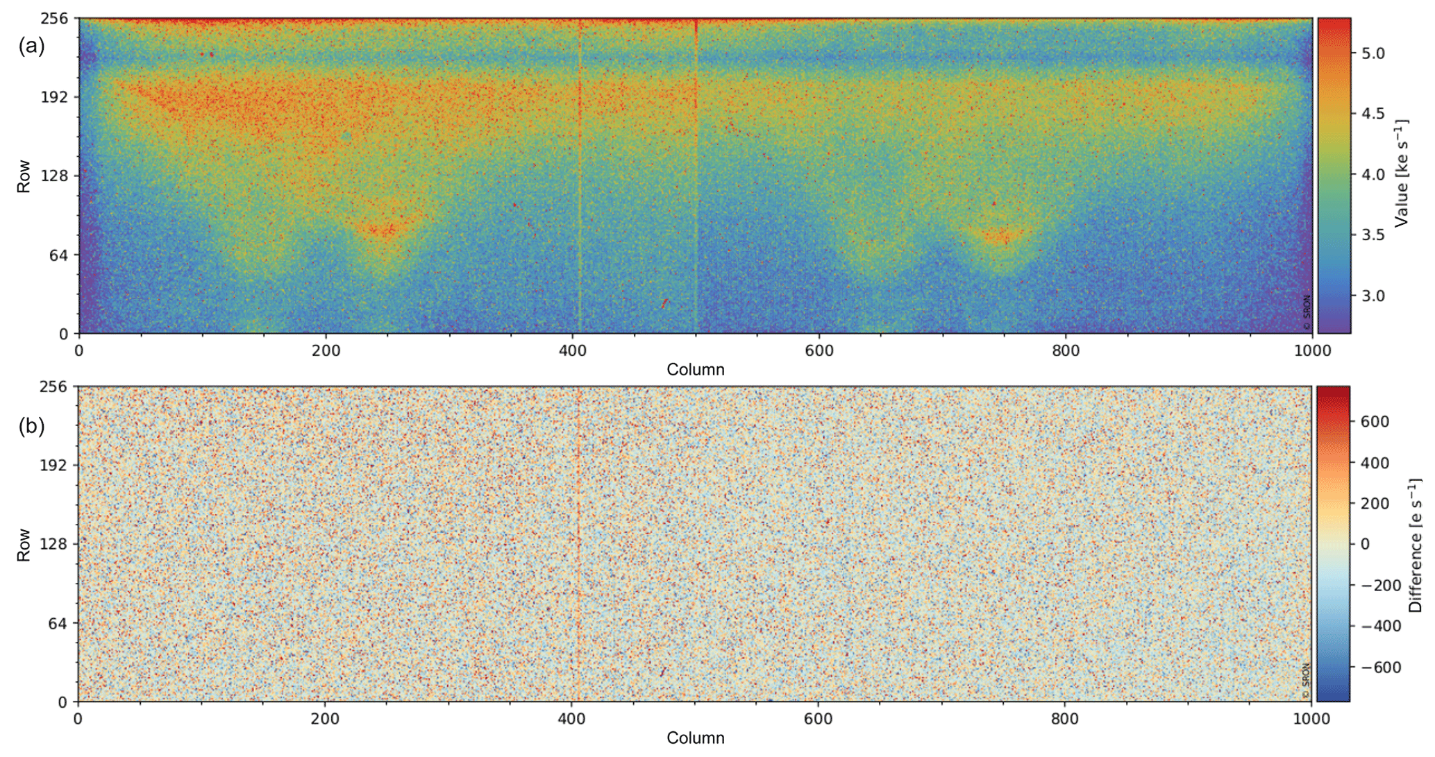
Figure 6The typical dark current obtained with the FMM closed at the start of the nominal operations phase using data from orbits 2818 to 2833 can be seen in panel (a). Data are plotted over the detector with the horizontal axis equivalent to the spectral direction and the vertical axis equivalent to the spatial swath. A comparisons to the dark current derived during the ground-based calibration is shown in panel (b).
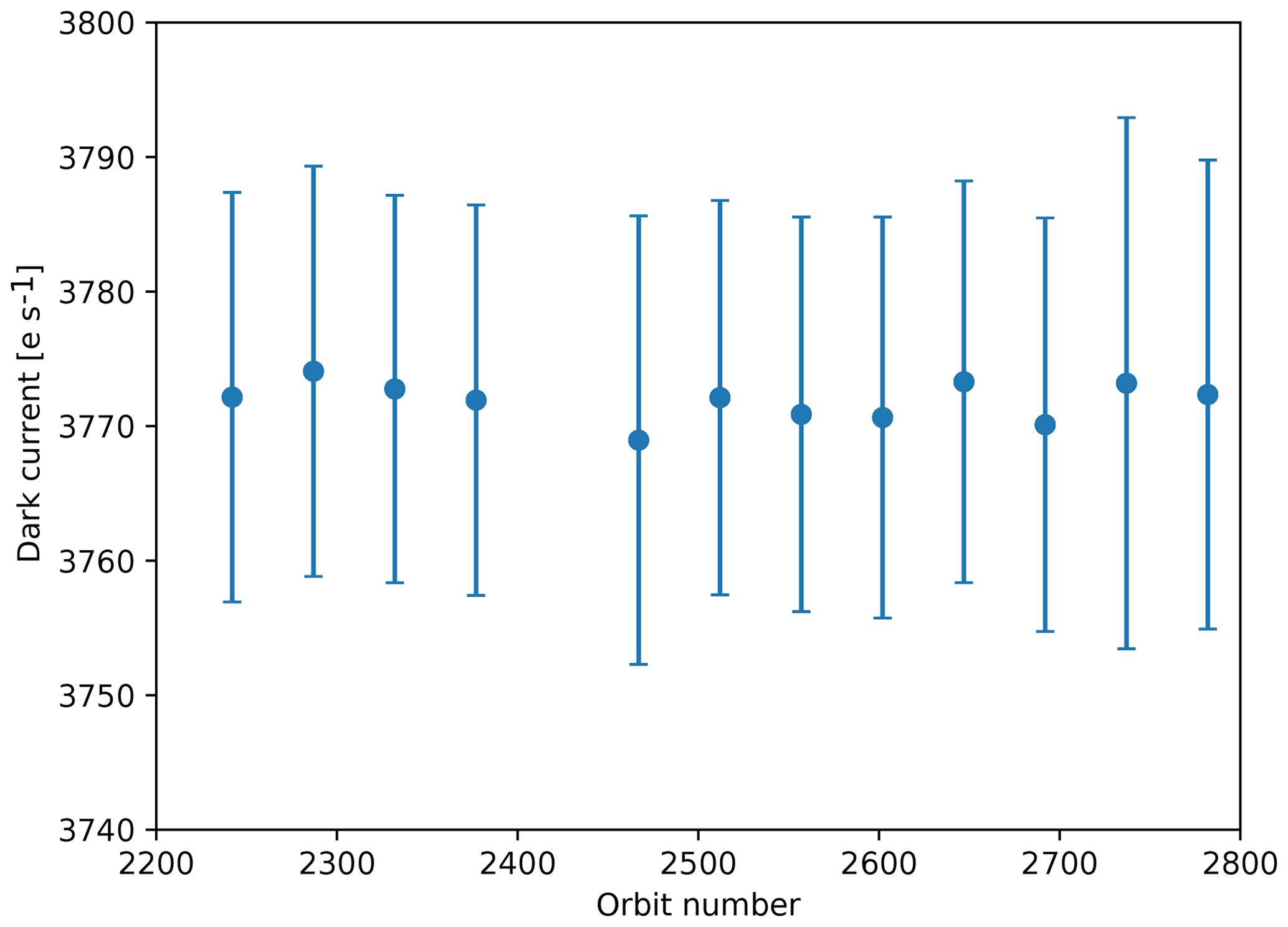
Figure 7The median dark current and its uncertainty obtained with the FMM closed at the start of the nominal operations phase between orbits 2200 to 2800 (the end of the commissioning phase) as a function of time. The length of time shown is about 6 weeks. Note that due to the structure seen in the dark current, the spread (not shown) is much larger.
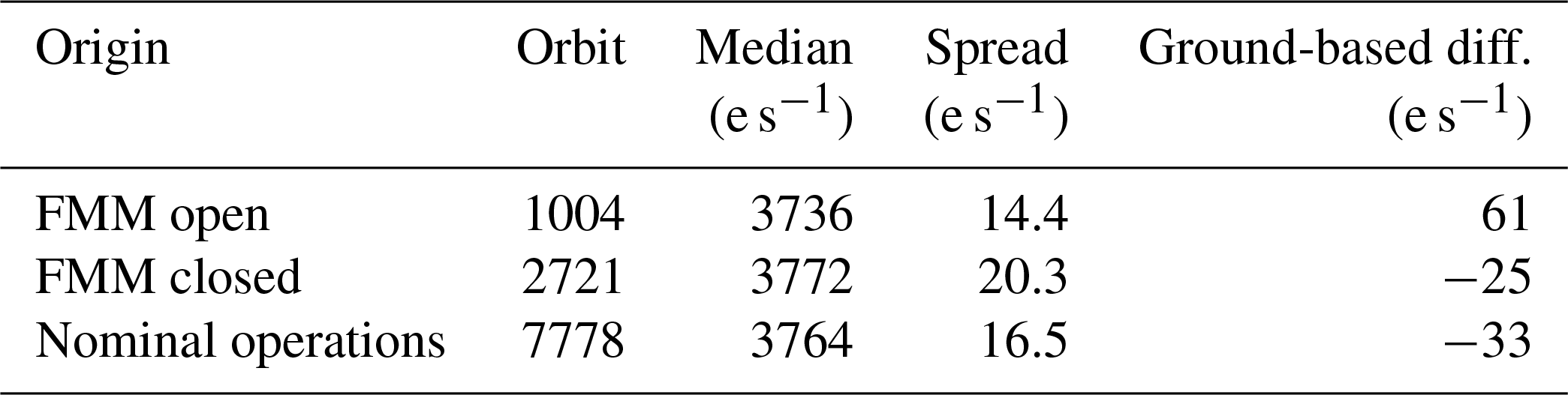
Table 2The median and spread of the various dark currents (nominal operations are with the FMM closed) and comparison with the median of the ground-based calibration. The difference is defined as the ground-based value minus the measurement. The ground-based results are based on many more measurements. As such, the uncertainties calculated from the spread are not comparable.
3.1.3 Dark current with the FMM closed
Given the issues described in Sect. 3.1.2, background measurements were also performed with the FMM closed.
Figure 6 shows the derived dark current with the FMM closed, and its comparison with the ground-based result. The detector median is given in Table 2. With the FMM closed, dark current does not differ significantly from the ground-based results.
Averaged over the entire detector, the dark current is ∼25 e s−1 lower than the ground-based measurements. This is likely due to different thermal conditions. Another difference to the ground-based results is found in the spread (i.e. the uncertainty of the fit). This is caused due to the number of input points for each fit. Both the number of different exposure times and the number of measurements available for each exposure time were higher during the ground-based calibration. However, the detected systematic differences between measurements on the ground and in-flight with the FMM open, such as the absorption bands or latitude-dependent signal are clearly absent when the FMM is closed.
The dark current with the FMM closed was also tracked in time over the last 2 months of the commissioning phase. Derivations were carried out at intervals of 15 orbits with the requirement that at least 40 % of all orbits contained background measurements. Figure 7 reveals that the dark current with the FMM closed is very stable with variations of 2–3 e s−1 from derivation to derivation. The uncertainty can vary depending on the total number and total length of the measurements included each interval.
3.1.4 Orbital dark
During nominal operations, measurements are typically taken at northern latitudes of the eclipse side of the orbit. As such, any variation within a single orbit cannot be monitored or calibrated. This may lead to a systematic error if there are thermal variations within a single orbit. Therefore, accurate calibration of the dark current includes a calibration of thermal variations as a function of the orbital phase7, using background measurements over a several orbits with the FMM closed. The observed signal with the FMM closed as a function of the orbital phase was inspected at exposure times of 100, 500, and 1000 ms. The data show no dependency of the dark current over the orbit. Therefore, no orbital variation of the dark-current correction is applied in the data processor. Two increases in the signal were detected, both during overpasses of the South Atlantic Anomaly (SAA) region. Within the SAA, the van Allen radiation belt dips much closer to the surface of the planet, significantly increasing the amount of cosmic radiation that hits the detector and leading to a small increase in the average background signal. All measurements in the SAA are flagged as less reliable.
3.1.5 Conclusions on the FMM setting
In conclusion, background measurements with the FMM closed produce more accurate and more stable dark currents than measurements with the FMM open. Surface features, such as fires and the land–sea difference, are removed from background measurements if the FMM is closed. In addition, the accidental introduction of spectral features due to methane and water absorption in the thermal radiation is also removed. When the data collected in the SAA are excluded from the analysis, no orbital dependency of the dark signal is necessary. Nominal operations were adapted to include this recommendation. The dark current is also shown to have similar values to those measured during the ground-based calibration as well as the values reported in the detector characterization (Hoogeveen et al., 2013).
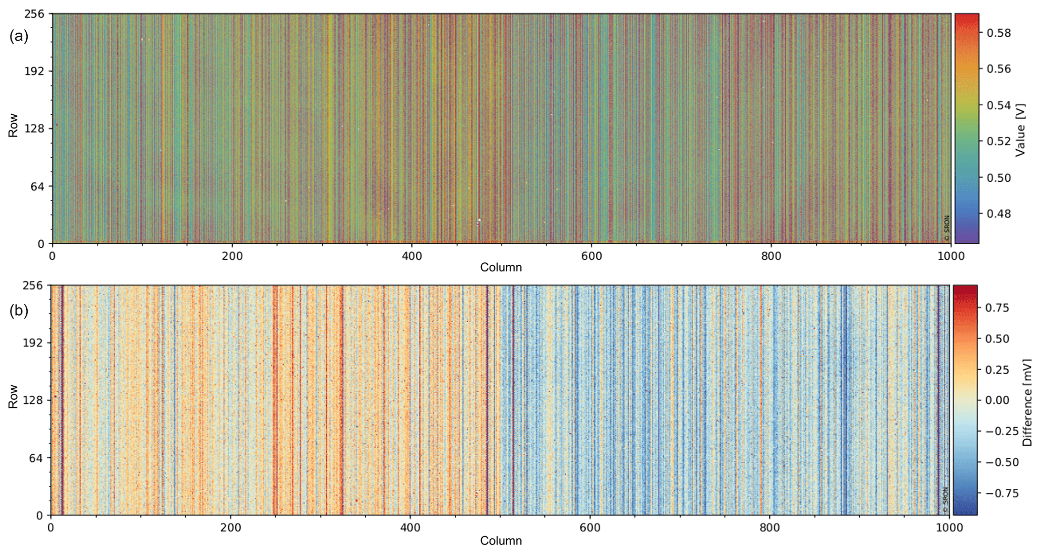
Figure 8The offset obtained with the FMM closed during the E1 phase using data from orbits 2707 to 2721 can be seen in panel (a). Data are plotted over the detector with the horizontal axis equivalent to the spectral direction and the vertical axis equivalent to the spatial swath. A comparison to the offset derived during the ground-based calibration is shown panel (b).
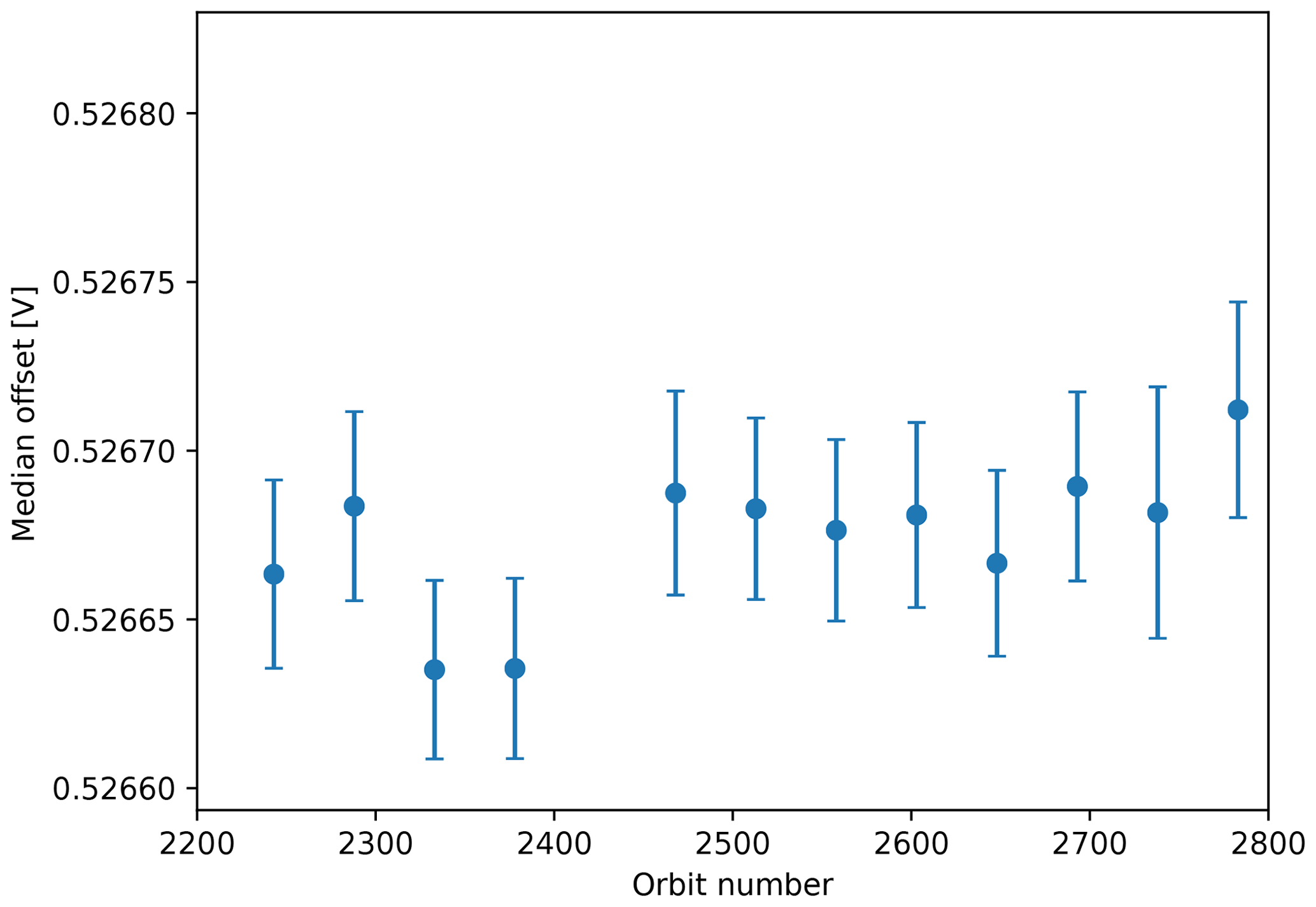
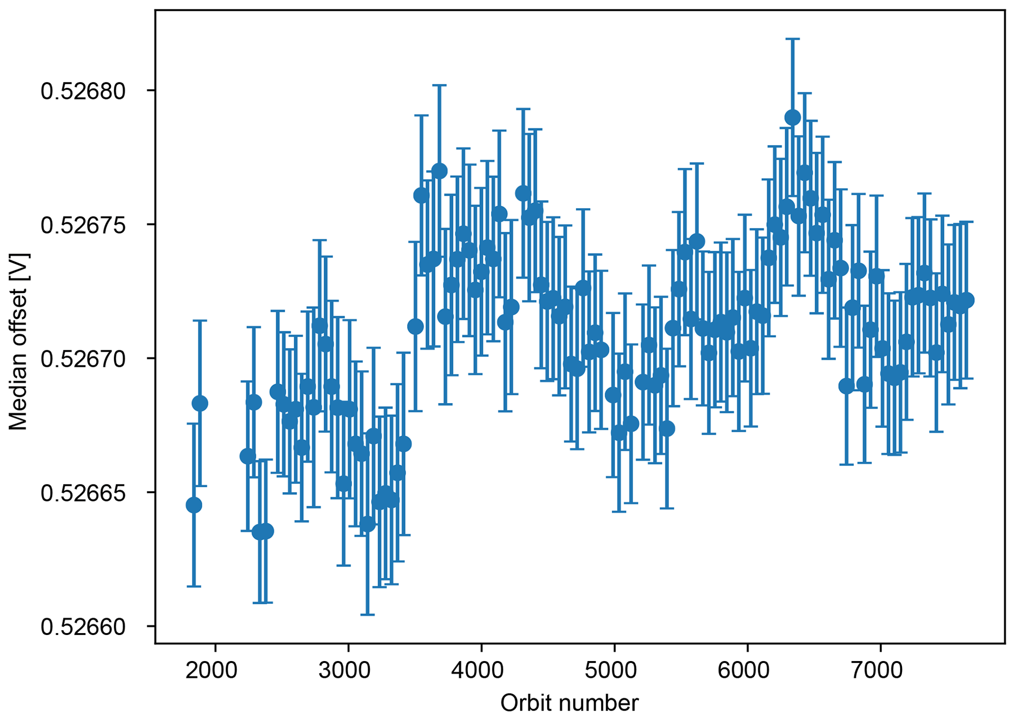
Figure 9The median offset and its uncertainty obtained with the FMM closed during the E1 phase between orbits 2200 to 2800 as a function of time.
3.1.6 Offset
As the offset is derived using the same set of measurements as the dark current, the offset of the SWIR detector shows similar dependencies to the dark current. All conclusions for the dark current also apply to the offset. Figures 8 and 9 show the offset with the FMM closed and its dependency on time as a reference. Note that a small systematic difference appears between the two analogue digital converters (ADC), each covering a half of the detector, which is not well understood, but is currently attributed to different thermal conditions. This difference is within the limits of the defined requirements.
3.2 In-flight noise
The noise on all signals read is composed of three components: (i) shot noises of the external signal, thermal background, and dark current; (ii) Johnson noise; and (iii) read noise. These combine to form the total noise. Read noise is independent of exposure time, whereas the other noise components depend on the exposure time. Read noise was calibrated during the ground-based calibration campaign by measuring the noise versus the exposure time and extrapolating back to zero exposure time. The other noise components are grouped as in-flight noise. It is necessary to measure the in-flight noise of each pixel without any external signal or its shot noise as input for the detector pixel quality monitoring. Detector pixels with overly high noise levels (either read noise or in-flight noise) are not used for the retrieval of CO or CH4.
Early in the E1 phase, in-flight noise calibration measurements were executed with the FMM open, similar to the dark current and offset. However, similar effects were seen for the noise as discussed in Sect. 3.1, with signals from point sources and nonuniform earthshine influencing the noise derivations. Therefore, calibration measurements to determine noise levels are also executed with the FMM closed during nominal operations.
Figure 10 shows the in-flight noise with the FMM closed, taken 6 months after launch. Noise can be derived either by taking the standard deviation over all frames within a measurement, with the median subtracted, or the spread of all frames. For a symmetric Gaussian distribution of the data points, both methods yield an identical result. But for a skewed distribution with outliers, the standard deviation method tends to result in a higher noise than the bi-weight median. In Fig. 10, both are plotted. For the SWIR module, most outliers are produced by cosmic-ray impacts that manifest themselves as dots and small tracks in Fig. 10.
Figure 11 shows the comparison between the read-noise CKD as measured on the ground and that measured in-flight. Figures are shown using derivations with a standard deviation and a bi-weight spread, highlighting the impact of cosmic rays.

Figure 10The noise of the SWIR detector measured during orbit 2707 to 2722 for an exposure time of 538.3 ms with the FMM closed, showing the noise calculated as a mean (a), median (b), and the difference between the two (c).
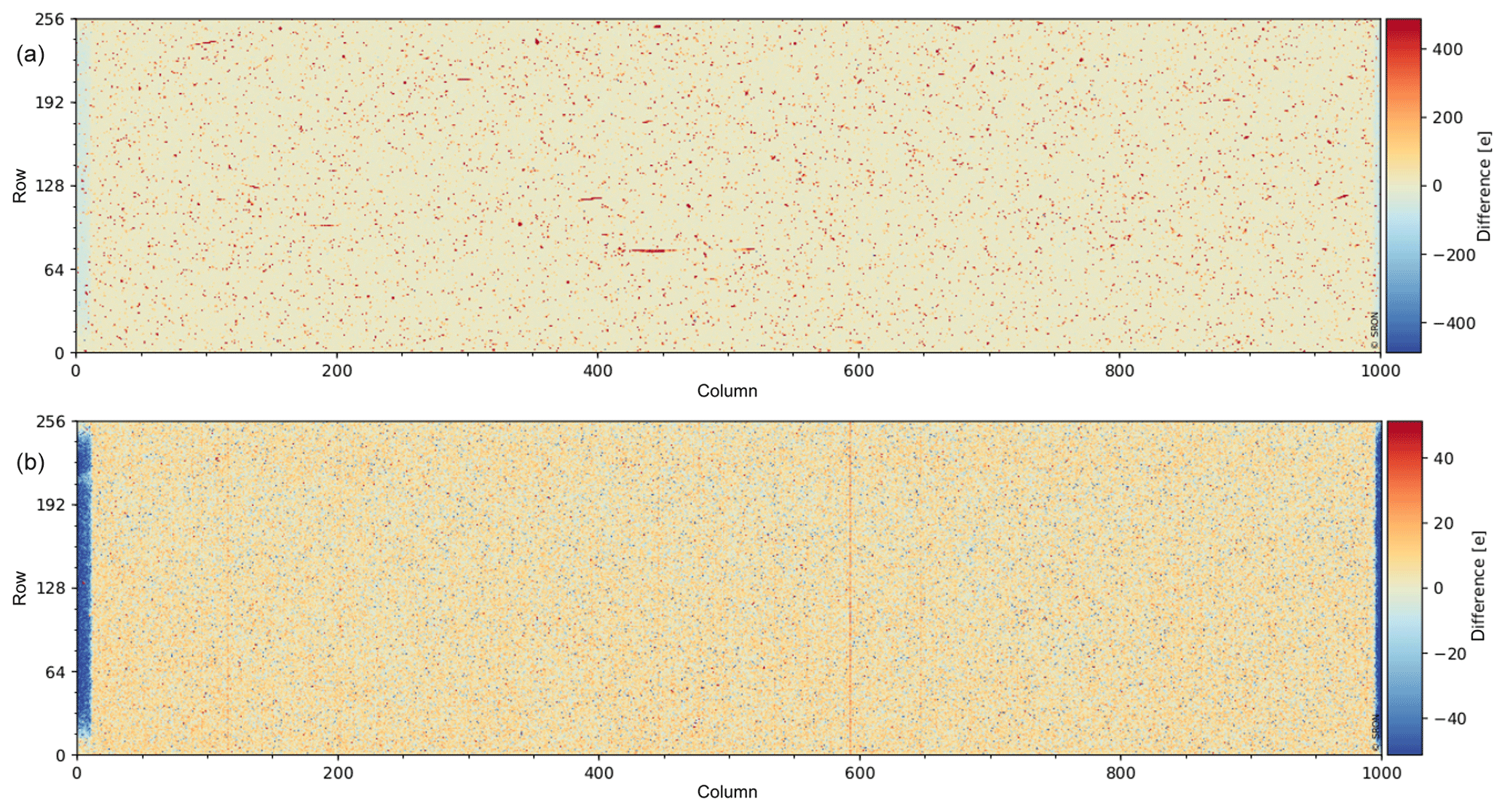
Figure 11Comparison between the noise measured in-flight during orbit 2707 to 2722 and that measured on the ground. Panel (a) shows the difference between derivations using a root mean square while panel (b) shows that using a bi-weight spread. Note that the similarity of the difference between ground-based and in-flight noise measurements and the difference between the two methods, as shown in Fig. 10c.
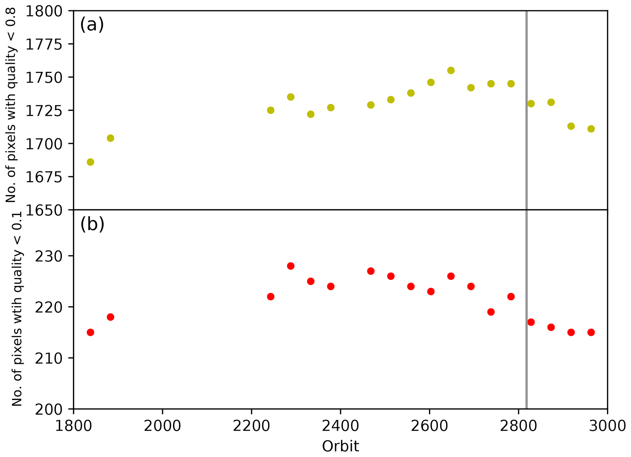
Figure 12Number of dead (b, red dots) and bad (a, yellow dots) pixels. The pixel quality is expressed as a number between 0 and 1. The dotted line is a linear fit through the data.
3.3 Detector pixel quality
The quality map of the SWIR detector details how many detector pixels are of sufficient quality to be included in retrieval algorithms. In the definition of “sufficient quality”, a pixel should
-
have a linear response to light as a function of exposure time,
-
not show excessive noise, and
-
not produce excessive dark current.
Excessive was defined as a spread that was more than three times higher than the median over the array. However, this definition will be reviewed in-flight. Using a weighted function (for which the weighting was determined using ground-based calibration measurements), each pixel is graded with a number between 0 (completely dead or unusable pixel) and 1 (perfectly working) using measurements of the noise and dark current. A detector pixel is considered to be bad if this value is lower than 0.8. A “dead” category is tracked by considering detector pixel with values below 0.18. If required, manual flagging is also possible within the processor (i.e. setting this quality to 0.0). Some pixels were known to be non-functional even before launch. For simplicity, the definition of non-functional includes pixels outside of the effective area that are not illuminated, but are technically functional. These were manually set to 0.0. Note that pixels are excluded from any trend plots such as Fig. 12. It is expected that other pixels may become unusable over time (e.g. no signal or too noisy) due to cosmic-ray impacts or hardware degradation.
Figure 12 shows the number of flagged pixels at the end of the commissioning period. Only data from orbit 1800 and later were analysed as data were collected using a consistent procedure with the FMM closed. An open FMM heavily influenced the dark and noise, and thus the quality. This quality map is derived using a bi-weight median noise, given the limitations discussed above. Table 3 lists the number of pixels identified both on the ground, during the commissioning phase, and at the start of nominal operations. Note that the quality is derived using all available data once per 15 orbits. Interestingly, the number of “bad” and “dead” pixels decreased after launch. This likely has several causes. First, the thermal environment during the ground-based calibration and the in-flight measurements (taken 1800 orbits after launch, which equates to over 4 months) is known to have been different. Second, the instrument settings of many of the ground-based calibration measurements were (subtly) different from those used in-flight. Third, the detector underwent an annealing as it was launched warm. Last but not least, the algorithm used to derive the offset and dark current was improved between the ground-based calibration and the end of E1.
Table 3Number of detector pixels labelled as “bad” (quality <0.8) or “dead” (quality < 0.1). Note that this does not cover the total 250 000 detector pixels. The area used for retrieval, and adopted above, equals approximately 210 000 pixels.

3.4 Transmission
The stability of the transmission of the optical components is checked by comparing the signal of various onboard calibration sources and the solar irradiance measured with the onboard diffusers. Although monitoring of the transmission of the full optical train for radiance measurements is the main goal, it can only be approximated with the methods applied. Changes seen in the signal of the calibration sources and/or solar irradiance signals can originate from degradation of the sources, diffusers, and/or any other optical elements in the optical path, including the video chain. Both the calibration sources and diffuser are expected to degrade over the operational lifetime. After cross-calibration, any changes in the transmission should be carefully monitored and investigated. In this section we will compare the output of the onboard calibration sources and compare it to the results obtained on the ground.

Figure 13DLED response of orbits 907 (a) and 2707 (b) relative to the in-flight reference of orbit 2515. Note that the change between orbits 2515 to 2707 is negligible.
3.4.1 DLED
The DLED is intended to monitor the stability of the detector. In-flight, monitoring of the detector signal caused by the DLED illumination is carried out by comparing the DLED response to a reference measurement taken late in the commissioning period. The reference measurement has, in turn, been calibrated to the ground-based reference.
Figure 13 shows the measurement of orbit 907 (December 2017) and 2707 (April 2018) compared with the reference measurement, which was set to the measurement from orbit 2515. The DLED responses, as seen in Fig. 13, already show that the DLED has degraded between orbits 907 and 2707 relative to the reference orbit of 2515. However, typical degradation can be seen at a level of 0.1 %. Features in the measurement of orbit 907 appeared after launch and then vanished, which is not well understood. It is hypothesized this is behaviour is either influenced by an etalon effect of a layer on the protective glass for the detector or a lens in the optical path of the DLED signal. The degradation is further discussed in Sect. 4.5.
3.4.2 WLS
A tungsten halogen lamp is mounted inside the calibration unit and acts as a white light source (WLS). Its output follows the complete light path within the module (see Fig. 1). The WLS settings have been optimized to yield sufficient signal in the UV and UVIS wavelengths. This results in a relatively strong output in the SWIR wavelength band. To avoid saturation, only measurements with a short exposure time (5 ms) are used for SWIR. The drawback is that due to small nonlinearity effects, the uncertainties of the pixel and/or full array cannot reliably be determined. A reference for the WLS was derived at the end of phase E1 during orbit 2513. Given the much less stringent stability limits of the WLS system, no differences were found in the resulting SWIR signals. Changes and/or the slight degradation seen in the SWIR signals of DLED fall within the measurement errors of an WLS measurement. This indicates that the optics of the SWIR module is stable over time.
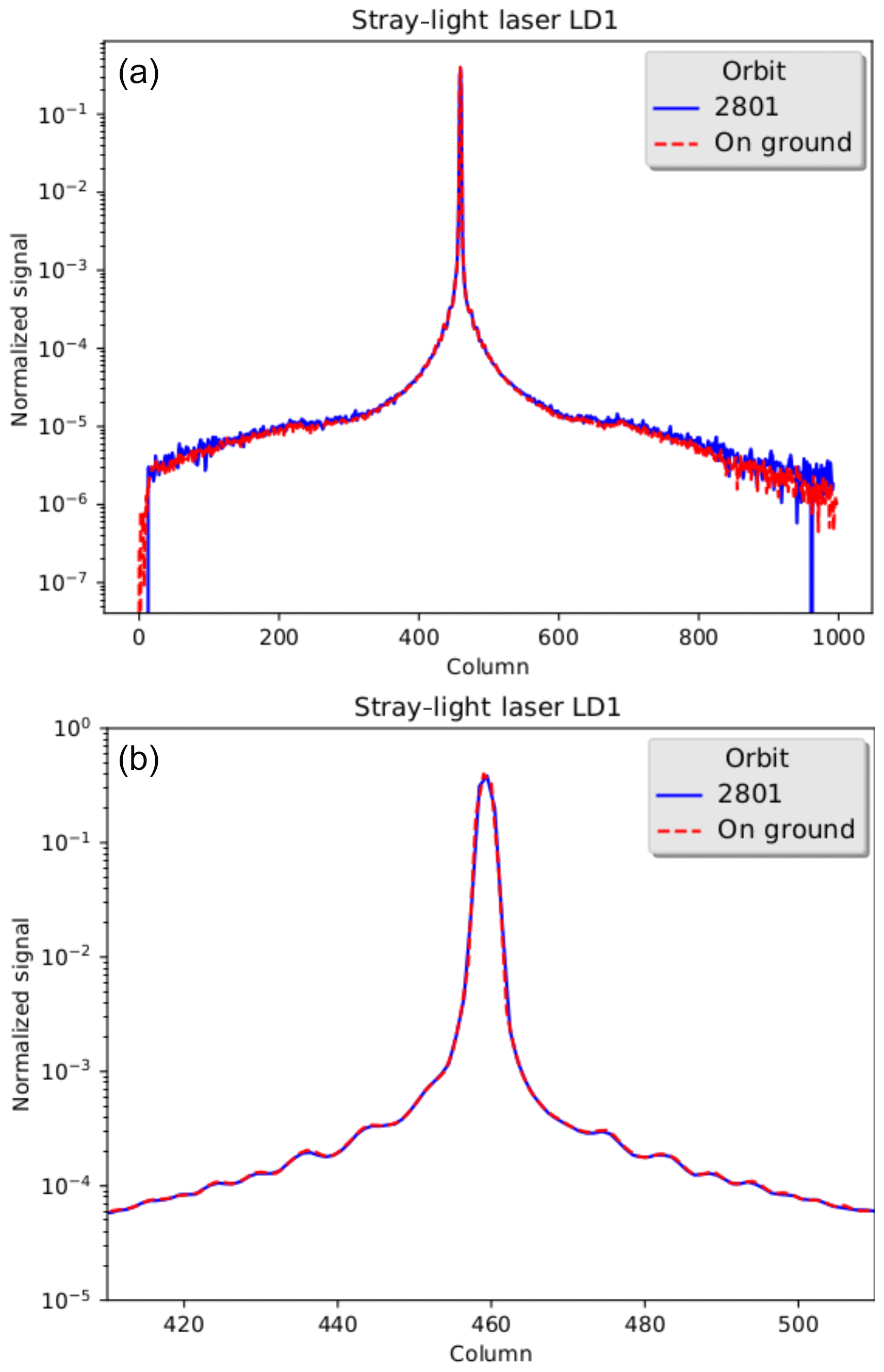
Figure 14Comparison of in-flight measurements using SLS-1 during a single orbit with an identical measurement obtained during ground-based calibration. Panel (a) shows the full image, and panel (b) shows a zoomed in section near the wavelength of SLS-1.
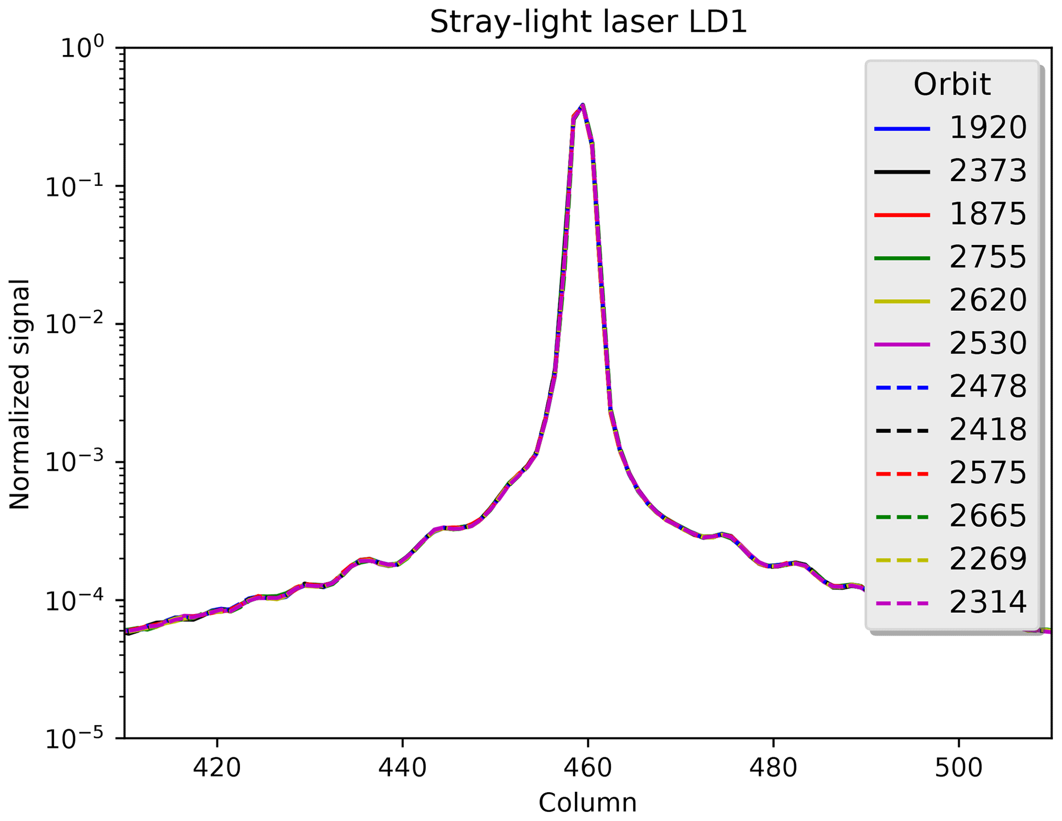
Table 4Percentage of light detected on the SWIR detector outside of the central 15 pixels of a response to diode laser SLS-1 during the E1 phase.

3.5 Stray light
The methodology to determine the stray-light calibration key data, including the ground-based measurements used, is described in detail in Tol et al. (2018). In-flight there is no capability to directly quantify the amount of stray light within the SWIR module as a response to a point source illuminating any location of the SWIR detector. However, there is the possibility to monitor the stability of the stray-light CKD over time by comparing the signal response of one of the onboard diode lasers that illuminates a spectral band with the equivalent ground-based measurement. Before launch, SLS-1 was selected for regular calibration measurements as its wavelength is located near the centre of the SWIR band. The effectiveness of the stray-light CKD is checked by comparing the known signal response of SLS-1. Monitoring is carried out by merging a short (98 ms) and long (1998 ms) exposure. Frame merging is discussed in Tol et al. (2018), Sect. 3. This method produces a frame with an unsaturated line centre while still retaining good signal-to-noise outer wings.
Figure 14 shows the spectral axis with medians taken over the swath for the ground-based and in-flight measurements for SLS-1. Stray light is normalized over the total signal. Both the full dynamic range and a zoom around the laser wavelength are shown. This reveals no changes before or after launch in the distribution of the stray light near the laser peak.
Figure 15 shows all measurements taken with SLS1 during the E1 phase, overlaid onto each other. This reveals that the amount and shape of stray light has remained stable over the course of the first few months after launch. This is confirmed by the tracking of the amount of stray light (seen in Table 4). The amount of stray light is defined as all light seen outside the 15 spectral pixels centred on the laser peak. Note that this is not a direct quantification of the stray light, but suffices as a monitoring quantity for the amount of stray light.

Figure 16Comparison between the ISRF measurements taken during the ground-based calibration campaign and the E1 phase. Panel (a) shows the normalized pixel response in-flight (red) and on the ground (blue). The residuals are plotted in green. Panel (b) shows a zoomed in section of the residuals.
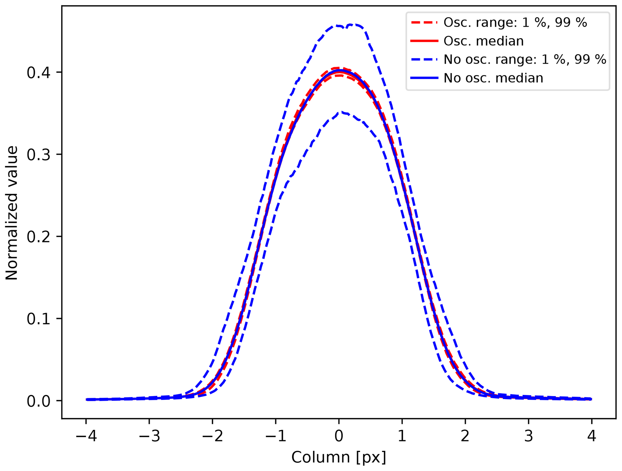
Figure 17Comparison between the ISRF measurements taken with and without an oscillating diffuser. The measurements with an oscillating diffuser are plotted in red and the measurements without an oscillating diffuser are plotted in blue.
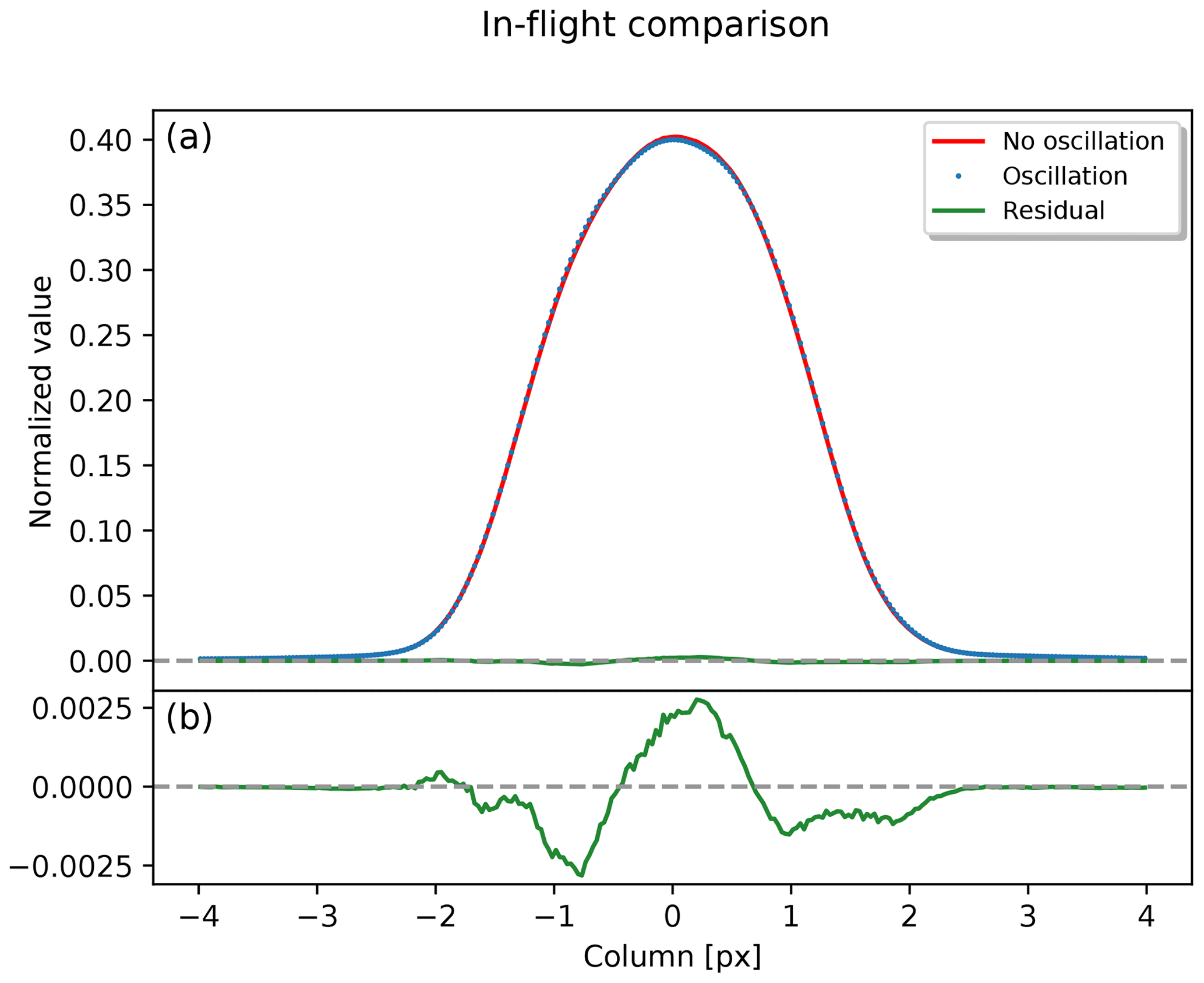
Figure 18Comparison between the ISRF measurements taken with and without an oscillating diffuser. In-flight measurements during nominal operations are carried out without an oscillating diffuser. Panel (a) shows the normalized pixel response in-flight (red) and on the ground (blue). The residuals are plotted in green. Panel (b) shows a zoomed in section of the residuals.
3.6 ISRF
The instrument spectral response function (ISRF) of each pixel is required as input data for the gas-retrieval algorithms. The complete method for deriving the ISRF CKD is described in van Hees et al. (2018). The CKD was derived using ground-based calibration measurements with an external tunable laser that had the capability to illuminate limited parts of the swath. A method was proposed in van Hees et al. (2018) to monitor the ISRF using the onboard diode lasers. Each diode laser illuminates a different area on the SWIR detector (and thus probes different parts of the ISRF spectral parameter range). A local “monitoring” ISRF is derived from these measurements. As the diode laser illuminates the full spatial swath and the five lasers only sample very small ranges of the full spectral axis, the diode lasers cannot be used to derive ISRF CKD. Their use is to detect and monitor long-term changes in the ISRF, if any. During the E1 phase, the results from van Hees et al. (2018) were verified to determine any possible changes between ground-based calibration and phase E1 performance. At the same time, a checkout was performed of the diode laser settings for use during nominal operations (E2). In this paper results from the diode laser SLS-1, which is the main reference during nominal operations, are presented, but all conclusions also apply to results obtained for the other four diode lasers.
Figure 16 shows the difference between measurements using diode laser SLS-1 carried out on the ground and in-flight. These were undertaken using identical settings. In this figure, the normalized pixel response is compared by taking a median over the illuminated swath (220 rows) and normalizing over the total energy. The difference observed between in-flight and ground-based measurements is less than 0.2 %, indicating no change in the instrument between the ground-based calibration and phase E1. The measurements were carried out with an oscillating diffuser.

During nominal operations, diode laser measurements are carried out using a fixed diffuser instead of an oscillating diffuser. The oscillation is needed to randomize the speckles of the monochromatic laser. However, as the diffuser motion is a life-limited item producing too much excess heat, it cannot be used during regular E2 monitoring. The resulting speckle pattern can be partially randomized by taking the median signal over all 220 rows illuminated. Figure 17 shows a comparison between in-flight measurements with identical settings except the (lack of) oscillation of the diffuser. In this plot the percentile range between 1 % and 99 % is shown for all ISRF solutions in the spatial direction. It is clear that the range of solutions is much larger without an oscillating diffuser. However, the median ISRF solutions of both sets of measurements are very similar. Figure 18 shows this difference. From this figure it can be confirmed that the measured profile without an oscillating diffuser, although less accurate than the actual ISRF, is of sufficient quality to monitor the stability of the ISRF calibration in-flight. The figures in this section reaffirm that no changes larger than 0.2 % are seen.
The performance of the SWIR module has been closely monitored since launch. At the end of phase E1, references were taken for the various monitoring parameters. In this section, the trends with respect to the reference are determined and are averaged over the full detector (i.e. either a mean or median of the properties over the detector or the total amount of pixels flagged over the detector). Interested readers are referred to the monitoring website of the SWIR module 9 for more information.
4.1 Background
Figures 19 and 20 show the detector median for the dark current and offset from 20 February 2018 to 30 April 2019. Both are extremely stable. Even on a per-pixel basis, variations are very small, on scales of a few electrons (or electrons per second in the case of dark current). Larger-scale variations seen during the monitoring have been exclusively caused by irregularities in the thermal controls, stemming from orbit manoeuvers (see http://www.sron.nl/tropomi-swir-monitoring/, last access: 17 December 2019, for case studies). An example is the gap around orbit 3500, caused by an anomalous fault in the spacecraft, which caused the entire instrument to heat up. Data during such manoeuvers are omitted from the data shown in Figs. 19 and 20.
4.2 Noise
Figure 21 shows the median noise of the SWIR detector as a function of time from 20 February 2018 for a year. There is some variation, but most is much smaller than the typical spread of the in-flight noise seen over the detector.
4.3 Detector pixel quality and radiation impacts
Radiation impacts will gradually degrade the detector by causing pixels to become too noisy for retrieval or damage them to such a degree that they stop functioning. Most of these impacts occur in the South Atlantic Anomaly.
Figure 22 shows the number of detector pixels flagged as bad or dead within the illuminated area from March 2018 to April 2019. Over this period, approximately 200 detector pixels had their quality value drop to below 0.8 and approximately 30 pixels dropped to below to below 0.1. A linear fit through all orbits gives a loss of 42 detector pixels per 1000 orbits in the category bad and 6 detector pixels per 1000 orbits in the category dead. When compared with the total amount of total pixels in the illuminated area (210 000 pixels), current estimates show that less than an additional 0.6 % will be bad or dead at the end of the envisioned 7-year lifetime of TROPOMI. It is good to note that this assumes detector pixels are lost at the – currently observed – linear rate of 0.1 % yr−1 However, if detector pixels are lost due to cumulative cosmic-ray impacts, the rate will likely become nonlinear at later stages during the instrument's lifetime. More in-depth analysis (i.e. using data from longer operational timescales) of the effects of cosmic-ray impacts is warranted and planned for future work.
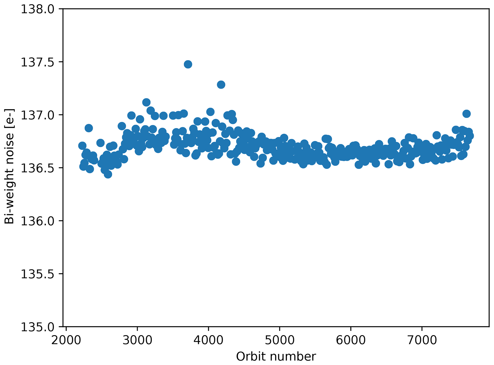
Figure 21Median noise as a function of time. Large instabilities have been removed from this trend. Note that the median noise is insensitive to cosmic-ray impacts.

Figure 22Number of bad (quality <0.8, a, yellow dots) and dead (quality <0.1, b, red dots) detector pixels since March 2018. A linear fit is shown using a black dashed line for each type. These have slopes of 42 and 6 detector pixels per 1000 orbits for bad and dead detector pixels respectively.
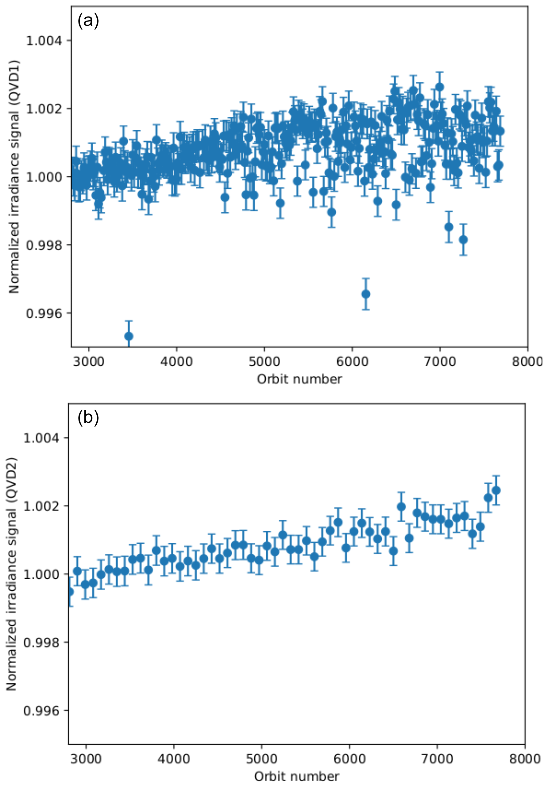
Figure 23Median normalized solar irradiance signal as a function of time. Panel (a) is the daily solar irradiance measurements, performed using the main diffuser QVD1. Panel (b) is the weekly solar irradiance measurement, performed using the backup diffuser QVD2.
4.4 Diffusers
Figure 23 shows the normalized response of the daily (which uses the main diffuser) or weekly (which uses the backup diffuser) solar irradiance measurements. Note that the diffusers are used for all four channels (UVN and SWIR) simultaneously. The diffusers do not appear to degrade at the SWIR wavelengths. However, a long-term variance can be seen in both diffusers, with both diffusers apparently becoming more effective. This is hypothesized to be due to either an uncalibrated factor in the relative irradiance or a change in reflectivity of the diffuser. The latter can be attributed to the diffuser degradation seen at short wavelengths (Quintus Kleipool, private communication, 2019) in one, but not the other. Last but not least, actual solar variance due to the solar minimum in 2018 may explain small differences. Further study in the form of very long-term monitoring is required to understand the observed slopes. As it is small, it has no observable effect on L2 products.

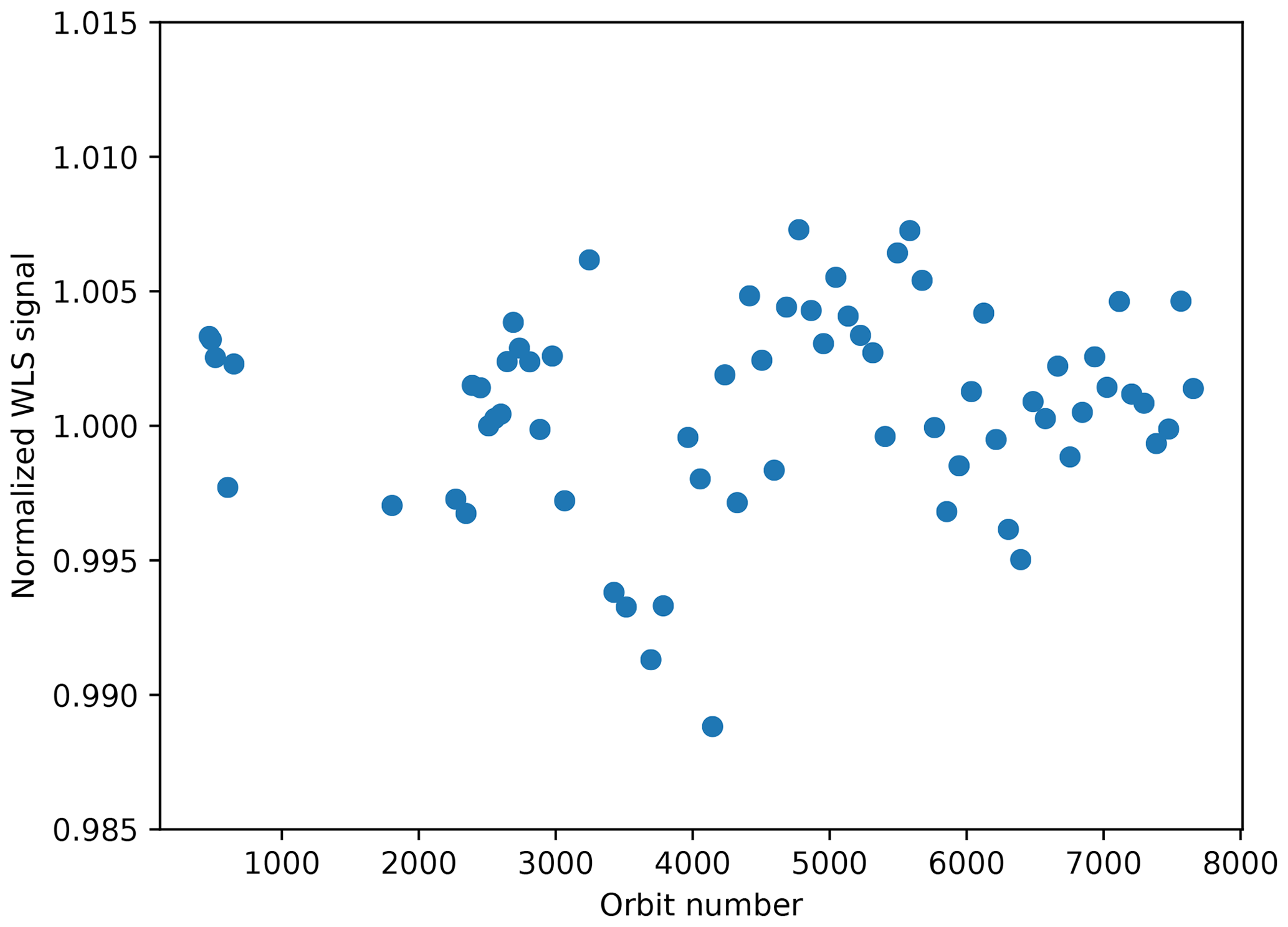
4.5 Stability of onboard calibration sources
Figures 24 and 25 show the normalized response of the DLED and WLS detector signals during nominal operations. The DLED signal is degrading at a rate of approximately 0.8 % yr−1. The voltage fed to the DLED has been completely constant over the mission so far. Given the increase of the solar irradiance signals, as seen in Fig. 23, it is thus concluded that the DLED itself is degrading and not the detector responsivity. However, more monitoring is required to confirm this hypothesis. Note that the outlier near orbit 3500 can be attributed to a spacecraft anomaly during which the entire instrument heated up.
The WLS signal appears not to degrade. Note, however, that the accuracy of the WLS measurements is limited. The output of the WLS varies within roughly 1 % (+0.5 %, −0.5 %), compared with the reference measurement. In addition, the spread of the values around the median of each measurement also varies from measurement to measurement. However, degradation at levels seen for the DLED can be ruled out. Thus, it confirms a DLED degradation.
If we assume that the DLED degrades linearly, and given the envisioned 7-year lifetime of TROPOMI, the DLED is expected to lose 6 % of its power output compared with the start of nominal operations.
4.6 ISRF
The stability of the ISRF is checked every month for each of the five diode lasers. Figure 26 shows the normalized pixel response in orbit 5396 compared with orbit 1667. Both measurements use identical settings. The difference is of the same order of magnitude as seen in the comparison with the ground-based measurements, reported earlier in Sect. 3.6. Monthly comparison reveal residuals of 0.2 % at most. These residuals vary from measurement to measurement due to the speckles on the diffuser.
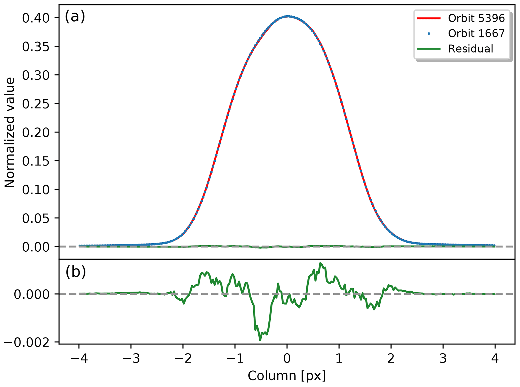
Figure 26Comparison between the ISRF measurements taken during the E1 phase and during nominal operations, both without an oscillating diffuser. Panel (a) shows the normalized pixel response in orbits 5396 (red) and 1667 (blue). The differences are plotted in green. Panel (b) shows a zoomed in section of the residuals.
4.7 Stray light
Stray-light monitoring is carried out once a month using the diode laser SLS-1. Figure 27 reaffirms the conclusions and trend seen during the E1 phase. Stray light is found to be very stable, with the amount of total stray light seen as a response to a line source being approximately 2.9 %.

From the results as presented in Sect. 3 of this paper, it can be concluded that the SWIR module did not change significantly between the ground-based calibration campaign and its first operations in space. This holds for all aspects: offset, dark current, detector noise, transmission, stray light, and ISRF. The results of the first year of nominal operations, as presented in Sect. 4 of this paper, show that the SWIR module is very stable indeed with respect to all aspects of the monitoring programme. During the few orbit manoeuvers that were needed to avoid collisions or to maintain formation flying with Suomi NPP, the orientation of the satellite was lost resulting in non-nominal temperatures on board. Recovery to nominal temperatures was found to take hours for the SWIR detector and up to days for the SWIR spectrometer. During this time, small deviations from the regular CKD may occur. Only if calibration measurements are scheduled can these be quantified. Data will be flagged in the data processer. The number of pixels that have been lost so far is negligible (about 200 over a full year have been found to be bad, and about 30 have been found to be dead), and given the current rate, less than 0.6 % of the total number of pixels will be lost over the envisioned operational time of 7 years, assuming a linear rate (which may not be true in case of accumulated radiation damage). With the condition of the TROPOMI-SWIR module as it is now, a very stable operational period is predicted with little to no changes foreseen for the processer and with respect to the calibration key data regarding SWIR products, yielding good quality Earth radiances to be used for accurate trace gas retrieval.
The results shown in this paper were derived using the calibration data obtained from calibration measurements on the ground and in-flight from Sentinel-5P. All data can be found in graphical form via links describing the calibration and validation activities: https://sentinel.esa.int/web/sentinel/technical-guides/sentinel-5p/calibration. Specific data are available upon request.
The authors declare that they have no conflict of interest.
The bulk of the work was carried out by TAvK, RMvH, and PJJT. RMvH was responsible for much of the analysis code, which was reviewed by PJJT and TAvK. The analysis was equally shared by the abovementioned authors. IA interacted with other TROPOMI specialist teams. RWMH supervised the team up until the end of the E1 phase.
This article is part of the special issue “TROPOMI on Sentinel-5 Precursor: first year in operation (AMT/ACPT inter-journal SI)”. It is not associated with a conference.
This paper contains Copernicus Sentinel data.
This research is funded by the TROPOMI national programme from the Netherlands Space Office (NSO).
This paper was edited by Ben Veihelmann and reviewed by four anonymous referees.
Beers, T. C., Flynn, K., and Gebhardt, K.: Measures of location and scale for velocities in clusters of galaxies – A robust approach, Astrophys. J., 100, 32–46, https://doi.org/10.1086/115487, 1990. a
Hoogeveen, R., Jongma, R., Tol, P., Gloudemans, A., Aben, I., Vries, J., Visser, H., Boslooper, E., Dobber, M., and Levelt, P.: Breadboarding activities of the TROPOMI-SWIR module – art. no. 67441T, Carbon, 6744, https://doi.org/10.1117/12.737892, 2007. a
Hoogeveen, R. W. M., Voors, R., Robbins, M. S., Tol, P. J. J., and Ivanov, I. T.: Characterization results of the TROPOMI Short Wave InfraRed detector, Proc. SPIE, 8889, https://doi.org/10.1117/12.2028759, 2013. a, b, c, d, e, f, g
Kleipool, Q., Ludewig, A., Babić, L., Bartstra, R., Braak, R., Dierssen, W., Dewitte, P.-J., Kenter, P., Landzaat, R., Leloux, J., Loots, E., Meijering, P., van der Plas, E., Rozemeijer, N., Schepers, D., Schiavini, D., Smeets, J., Vacanti, G., Vonk, F., and Veefkind, P.: Pre-launch calibration results of the TROPOMI payload on-board the Sentinel-5 Precursor satellite, Atmos. Meas. Tech., 11, 6439–6479, https://doi.org/10.5194/amt-11-6439-2018, 2018. a, b
Tol, P. J. J., van Kempen, T. A., van Hees, R. M., Krijger, M., Cadot, S., Snel, R., Persijn, S. T., Aben, I., and Hoogeveen, R. W. M.: Characterization and correction of stray light in TROPOMI-SWIR, Atmos. Meas. Tech., 11, 4493–4507, https://doi.org/10.5194/amt-11-4493-2018, 2018. a, b, c, d
van Hees, R. M., Tol, P. J. J., Cadot, S., Krijger, M., Persijn, S. T., van Kempen, T. A., Snel, R., Aben, I., and Hoogeveen, Ruud W. M.: Determination of the TROPOMI-SWIR instrument spectral response function, Atmos. Meas. Tech., 11, 3917–3933, https://doi.org/10.5194/amt-11-3917-2018, 2018. a, b, c, d, e, f
Veefkind, J. P., Aben, I., McMullan, K., Förster, H., de Vries, J., Otter, G., Claas, J., Eskes, H. J., de Haan, J. F., Kleipool, Q., van Weele, M., Hasekamp, O., Hoogeveen, R., Landgraf, J., Snel, R., Tol, P., Ingmann, P., Voors, R., Kruizinga, B., Vink, R., Visser, H., and Levelt, P. F.: TROPOMI on the ESA Sentinel-5 Precursor: A GMES mission for global observations of the atmospheric composition for climate, air quality and ozone layer applications, Remote Sens. Environ., 120, 70–83, https://doi.org/10.1016/j.rse.2011.09.027, 2012. a, b
see http://www.copernicus.eu (last access: 17 December 2019)
TROPOMI is a collaboration between Airbus Defence and Space Netherlands, KNMI (Koninklijk Nederlands Meteorologisch Instituut), SRON (Netherlands Institute for Space Research), and TNO (Nederlandse Organisatie voor Toegepast Natuurwetenschappelijk Onderzoek), on behalf of NSO (Netherlands Space Office) and ESA (European Space Agency). Airbus Defence and Space Netherlands is the main contractor for the design, building, and testing of the instrument. KNMI and SRON are the principal investigator institutes for the instrument. TROPOMI is funded by the following ministries of the Dutch government: the Ministry of Economic Affairs; the Ministry of Education, Culture and Science; and the Ministry of Infrastructure and the Environment.
The SWIR spectrometer was developed by SSTL (Surrey Satellite Technology Ltd.) under an Airbus–Dutch Space contract, with contributions from SRON and Sofradir.
Note that a CLED is within the light path of the SWIR detector (Kleipool et al., 2018). However, the emission properties of the CLED show that it does not emit any light at SWIR wavelengths and is thus not relevant for SWIR calibration.
Note in this paper, we define the dark current as the combination of the true dark current (i.e. the current produced by the detector at its operational temperature) and the signal from the thermal background of the surrounding instrument components.
Throughout this paper, the bi-weight median and bi-weight spread are used. For simplicity the terms median and spread are used throughout. The bi-weight median is a statistical parameter described in Beers et al. (1990).
Orbital phase is a number between 0 and 1 defining the point after orbital midnight at which the spacecraft is located within a single orbit.
Note that the dead category includes, but is not limited to, pixels with no response (i.e. a value of 0.0). “Dead” pixels with a nonzero quality grading can improve to a higher grading such as “bad” and are thus not truly dead. However, for simplicity, we have limited ourselves to these three categories.
http://www.sron.nl/tropomi-swir-monitoring/ (last access: 17 December 2019)
- Abstract
- Introduction
- In-flight calibration and monitoring plan
- In-flight calibration during the commissioning phase
- Monitoring results during nominal operations
- Conclusions
- Data availability
- Competing interests
- Author contributions
- Special issue statement
- Acknowledgements
- Financial support
- Review statement
- References