the Creative Commons Attribution 4.0 License.
the Creative Commons Attribution 4.0 License.
 | 06 Mar 2020
Increasing the spatial resolution of cloud property retrievals from Meteosat SEVIRI by use of its high-resolution visible channel: evaluation of candidate approaches with MODIS observations
Hartwig Deneke
This study presents and evaluates several candidate approaches for downscaling observations from the Spinning Enhanced Visible and Infrared Imager (SEVIRI) in order to increase the horizontal resolution of subsequent cloud optical thickness (τ) and effective droplet radius (reff) retrievals from the native spatial resolution of the narrowband channels to . These methods make use of SEVIRI's coincident broadband high-resolution visible (HRV) channel. For four example cloud fields, the reliability of each downscaling algorithm is evaluated by means of collocated 1 km×1 km MODIS radiances, which are reprojected to the horizontal grid of the HRV channel and serve as reference for the evaluation. By using these radiances, smoothed with the modulation transfer function of the native SEVIRI channels, as retrieval input, the accuracy at the SEVIRI standard resolution can be evaluated and an objective comparison of the accuracy of the different downscaling algorithms can be made. For the example scenes considered in this study, it is shown that neglecting high-frequency variations below the SEVIRI standard resolution results in significant random absolute deviations of the retrieved τ and reff of up to ≈14 and ≈6 µm, respectively, as well as biases. By error propagation, this also negatively impacts the reliability of the subsequent calculation of liquid water path (WL) and cloud droplet number concentration (ND), which exhibit deviations of up to and , respectively. For τ, these deviations can be almost completely mitigated by the use of the HRV channel as a physical constraint and by applying most of the presented downscaling schemes. Uncertainties in retrieved reff at the native SEVIRI resolution are smaller, and the improvements from downscaling the observations are less obvious than for τ. Nonetheless, the right choice of downscaling scheme yields noticeable improvements in the retrieved reff. Furthermore, the improved reliability in retrieved cloud products results in significantly reduced uncertainties in derived WL and ND. In particular, one downscaling approach provides clear improvements for all cloud products compared to those obtained from SEVIRI's standard resolution and is recommended for future downscaling endeavors. This work advances efforts to mitigate impacts of scale mismatches among channels of multiresolution instruments on cloud retrievals.
- Article
(9222 KB) - Full-text XML
- Companion paper
- BibTeX
- EndNote


In studies of the role of clouds in the climate system, the bispectral solar reflective method described by Twomey and Seton (1980), Nakajima and King (1990), and Nakajima et al. (1991) is widely used to infer cloud optical and physical properties from satellite-based sensors. Based on observations of solar reflectance (r) from a channel pair at wavelengths with conservative scattering (usually around 0.6 or 0.8 µm) and significant absorption by cloud droplets (common channels are 1.6, 2.2, and 3.7 µm), respectively, this method simultaneously estimates the cloud optical depth (τ) and effective droplet radius (reff) of a sampled cloudy pixel. This method however relies on a number of assumptions which are often violated in nature: clouds are considered to be horizontally homogeneous and to have a prescribed vertical structure, which is generally assumed to be vertically homogeneous or to show a linear increase of liquid water content as predicted by adiabatic theory (see the discussions in Brenguier et al., 2000, and Miller et al., 2016). Moreover, the observed cloud top reflectance field is usually described by one-dimensional (1-D) plane-parallel radiative transfer, which neglects horizontal photon transport between neighboring atmospheric columns.
Use of the independent pixel approximation (IPA; see Cahalan et al., 1994a, b) produces uncertainties in the retrieved cloud variables that are dependent upon the horizontal resolution of the observing sensor. For sensors with a high spatial resolution, the observations resolve the actual cloud heterogeneity, which are unaccounted for in the IPA approach. This usually results in an overestimation of both τ and reff, as reported in Barker and Liu (1995), Chambers et al. (1997), and Marshak et al. (2006). Conversely, for observations with a low spatial resolution, the actual cloud heterogeneity cannot be resolved. Moreover, the chances of clear-sky contamination within a cloudy pixel increase with increasing spatial resolution. As a result, an underestimation (overestimation) of retrieved τ (reff) is usually observed (Marshak et al., 2006; Zhang and Platnick, 2011; Zhang et al., 2012; Werner et al., 2018b). These uncertainties are propagated to the liquid water content (WL) and the droplet number concentration (ND), which can be estimated from retrieved τ and reff. Estimates of ND are especially susceptible to uncertainties in reff, which impacts the reliability of aerosol–cloud-interaction studies (Grosvenor et al., 2018). The analysis in Varnai and Marshak (2001) suggests that a horizontal scale of around 1–2 km minimizes the combined uncertainty from unresolved and resolved cloud heterogeneity. While strategies to mitigate the effects of unresolved cloud variability have been recently reported in Zhang et al. (2016) and Werner et al. (2018a), these techniques become less successful with lower-resolution sensors like those operated on geostationary satellites.
Remote sensing from geostationary platforms such as the Meteosat Spinning Enhanced Visible and Infrared Imager (SEVIRI) offers unique capabilities for cloud studies not available from polar-orbiting satellites. These advantages include more frequent temporal sampling of individual regions and the ability to capture the temporal evolution (Bley et al., 2016; Senf and Deneke, 2017) and diurnal cycle of cloud parameters (Stengel et al., 2014; Bley et al., 2016; Martins et al., 2016; Seethala et al., 2018). However, SEVIRI pixels are characterized by a lower spatial resolution of its narrow-band channels compared to other operational remote sensing instrumentation, like the Moderate Resolution Imaging Spectroradiometer (MODIS, Platnick et al., 2003) or the Visible Infrared Imaging Radiometer Suite (VIIRS, Lee et al., 2006). Given the increase in retrieval uncertainty due to the IPA constraints, there is a desire to increase the resolution for geostationary cloud observations.
The aim of this paper is to critically evaluate several candidate approaches for downscaling of the SEVIRI narrow-band reflectances for operational usage and to identify the most promising of these schemes, exploiting the fact that information on small-scale variability is available from its broadband high-resolution visible (HRV) channel. The study by Deneke and Roebeling (2010) presented a statistical downscaling approach of the SEVIRI channels in the visible to near-infrared (VNIR) spectral wavelength range. This method makes use of the fact that SEVIRI's high-resolution channel can be modeled by a linear combination of the 0.6 and 0.8 µm channels with good accuracy (Cros et al., 2006). This study advances these efforts in three ways: (i) it explores other possible downscaling approaches, which might improve upon the statistical downscaling scheme; (ii) it introduces techniques to accurately capture information on the small-scale reflectance variability in the 1.6 µm channel, which predominantly arises from variations in effective droplet radius; and (iii) it studies the impact of the various downscaling techniques on the subsequently retrieved cloud properties.
A critical requirement, formulated at the start of this work, is to maintain a target accuracy for the retrieved effective radius based on the lower-resolution observations, while hoping for further improvements. This goal was set because the error in effective radius will propagate into other cloud products such as vertically integrated liquid or ice water path or the cloud droplet number concentration, thereby potentially corrupting any gains in accuracy obtained from the improved spatial resolution. However, without an independent reference data set, it is impossible to determine whether this target can be met. Thus, higher-resolution reflectance observations from Terra MODIS are remapped to SEVIRI’s HRV and standard-resolution grids here as basis for a thorough evaluation of the accuracy of the retrieved cloud parameters. This allows us to objectively benchmark the accuracy of candidate approaches by comparison of results from a true ≈1 km resolution reflectance data set and processed with an identical retrieval scheme. Note that even the retrieved cloud products from a hypothetically perfect downscaling technique would still be impacted by the effects of resolved and unresolved cloud variability. Therefore, the results of this study will not help to mitigate the uncertainties associated with the retrieval schemes of similar ≈1 km sensors (e.g., clear-sky contamination, plane-parallel albedo bias, three-dimensional radiative effects).
The results of this study are relevant for many other passive satellite sensors, which, like the SEVIRI instrument, feature multiple resolutions for the conservative and absorbing channels. Similar configurations exists for the MODIS instrument (250 m horizontal resolution versus 500 m for the 0.6 and 2.1 µm channels, respectively), VIIRS (375 m versus 750 m), and GOES-R (500 m versus 1 km).
The structure of the paper is as follows: Sect. 2 describes both the SEVIRI and MODIS instruments used as basis for this study, as well as the covered observational domain. A brief overview of the SEVIRI cloud property retrieval algorithm is given in Sect. 3, followed by a description of the different candidate approaches for the downscaling of the narrow-band SEVIRI channel observations in Sect. 4. An example of lower- and higher-resolution cloud property retrievals is presented in Sect. 5. A statistical evaluation of the different downscaling approaches based on remapped MODIS observations follows in Sect. 6 for a limited number of example cloud fields. Finally, a comparison between a full downscaling scheme and a VNIR-only approach (similar to Deneke and Roebeling, 2010) is given in Sect. 7. The paper presents the main conclusions and an outlook in Sect. 8.
This section gives an overview of both the SEVIRI and MODIS instruments in Sect. 2.1 and 2.2. Here, the respective spectral channels of interest for this study are listed. Subsequently, the observational domain is described in Sect. 2.3.
2.1 SEVIRI
The current version of European geostationary satellites is the Meteosat Second Generation, which has provided operational data since 2004 (Schmetz et al., 2002). The SEVIRI imager is installed aboard the Meteosat-8 to Meteosat-11 platforms, which are positioned above longitudes of 9.5∘ E and 0.0∘, respectively. One SEVIRI instrument samples the full disk of the Earth from 0.0∘ longitude with a temporal resolution of 15 min. However, a backup satellite positioned at 9.6∘ E also scans a northern subregion with a temporal resolution of 5 min (the so-called Rapid Scan Service). These samples – in our case from Meteosat-9 – provide the observational SEVIRI data set for the following analysis.
This study mainly considers observations from SEVIRI's solar reflectance channels 1–3, as well as from the spectrally broader HRV band. These channels cover the VNIR and shortwave-infrared (SWIR) spectral wavelength ranges. The two VNIR reflectances (r06 and r08) are sampled in bands 1 and 2, respectively, and are centered around wavelengths λ=0.635 and λ=0.810 µm. SWIR reflectances (r16) are provided by channel 3 observations, which are centered around λ=1.640 µm. The horizontal resolution of the channel 1–3 samples is 3 km×3 km at the subsatellite point and increases with higher sensor zenith angles. Conversely, the broadband reflectances rHV are sampled at SEVIRI's HRV channel at a horizontal scale of 1 km×1 km at the subsatellite point. These observations cover the spectral range of 0.4–1.1 µm.
As context for the present study, the reader is reminded that the spatial resolution of geostationary satellites is significantly reduced at higher latitudes due to the oblique viewing geometry. For Germany and Central Europe as considered in this paper, the pixel size is effectively increased by a factor of 2 in the north–south direction as a result. In addition, the distinction between sampling and optical resolution needs to be acknowledged. While the former determines the distance between recorded samples, the latter is given by the effective area of the optical system, which is larger by a factor of 1.6 than the sampling resolution for SEVIRI (Schmetz et al., 2002). The spatial response of optical systems is commonly characterized by their modulation transfer function, which describes the response of the optical system in the frequency domain.
Further information about the spectral width of each SEVIRI channel, as well as the respective spatial response and modulation transfer functions, can be found in Deneke and Roebeling (2010).
2.2 Terra MODIS
The 36-band scanning spectroradiometer MODIS, which was launched aboard NASA’s Earth Observing System satellites Terra and Aqua, has a viewing swath width of 2330 km, yielding global coverage every 2 d. MODIS collects data in the spectral region between 0.415 and 14.235 µm, covering the VNIR to thermal-infrared spectral wavelength range. In general, the spatial resolution at nadir of a MODIS pixel is 1000 m for most channels, although the pixel dimensions increase towards the edges of a MODIS granule. Only observations from the Terra satellite launched in 1999 are used here, due to broken detectors of the 1.64 µm channel of the MODIS instrument on the Aqua satellite. Information on MODIS and its cloud product algorithms is given in Ardanuy et al. (1992), Barnes et al. (1998), and Platnick et al. (2003). The current version of the level 1b radiance and level 2 cloud products used is data collection 6.1 (C6.1).
2.3 Domain
In this study, data from a subregion of the full SEVIRI disk has been selected. This region, which is located within the European subregion described in Deneke and Roebeling (2010), is illustrated by the red borders in Fig. 1. It is centered around Germany due to its intended domain of application (thus, from here on it is referred to as the Germany domain) and comprises the latitude and longitude ranges of ≈44.30–57.77∘ and –21.65∘, respectively. This domain includes 240×400 lower-resolution pixels (i.e., the native SEVIRI resolution of channels 1–3) and is far away from the edges of the full SEVIRI disk, ensuring that the observed viewing zenith angles are .
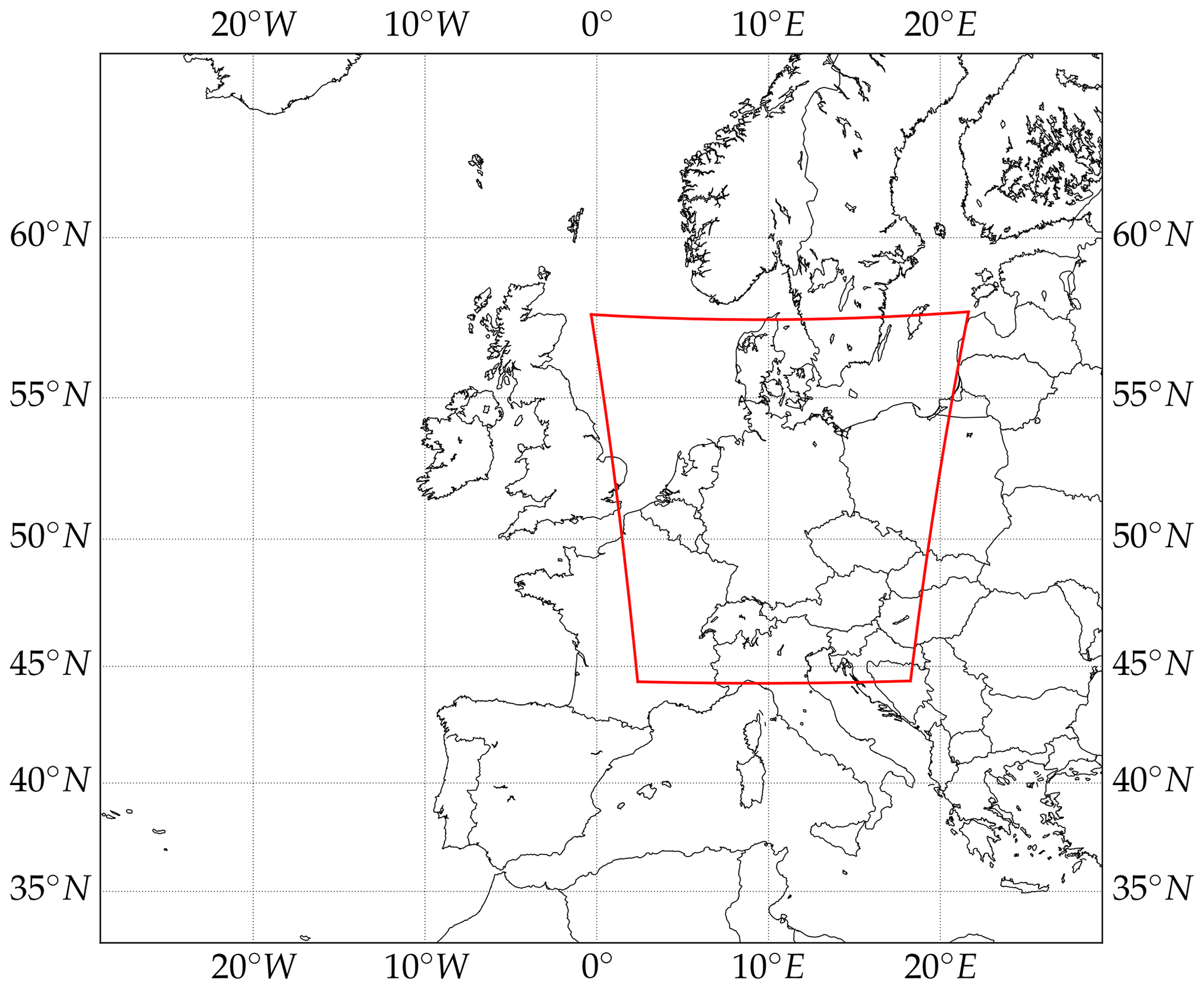
Figure 1Map of the European SEVIRI domain, as defined in Deneke and Roebeling (2010). The red borders indicate the Germany domain, which is the focus of this study.
Due to the increased sensor zenith angles the spatial resolution of each SEVIRI pixel is degraded. The average pixel size is 6.20 km×3.22 km and 2.06 km×1.07 km for channels 1–3 and the HRV channel, respectively. To avoid confusion, we will use the designations LRES (abbreviation for lower resolution) and HRES (abbreviation for higher resolution) scales to refer to the 3 km×3 km and 1 km×1 km pixel resolutions from here on.
A relatively small domain was chosen, because the number of pixels to be processed will expand by a factor of 3×3, increasing the computational costs of the subsequent cloud property retrievals by roughly 1 order of magnitude. Except for some regional dependencies introduced by changes in the prevalence of specific cloud types, we expect results of our study to also be valid for other domains.
Retrieved cloud variables in this study are provided by the Cloud Physical Properties retrieval algorithm (CPP; Roebeling et al., 2006), which is developed and maintained at the Royal Netherlands Meteorological Institute (KNMI). It is used as basis for the CLAAS-1 and CLAAS-2 climate data records (Stengel et al., 2014; Benas et al., 2017) distributed by the Satellite Application Facility on Climate Monitoring (Schulz et al., 2009). Using a lookup table (LUT) of reflectances simulated by the Doubling–Adding KNMI (DAK: , ) radiative transfer model, observed and simulated reflectances at 0.6 and 1.6 µm are iteratively matched to yield estimates of τ and reff. The CPP retrieval uses the cloud mask and cloud top height products obtained from the software package developed and distributed by the satellite application facility of Support to Nowcasting and Very Short Range Forecasting (NWCSAF), version 2016, as input (Le Gléau, 2016). The former product identifies cloudy pixels for the retrieval, while the information on the height of the cloud is used to account for the effects of gas absorption in the SEVIRI channels.
This section describes the necessary steps to convert the reflectances r06, r08, and r16, available at SEVIRI's native LRES, to reliable estimates of higher-resolution reflectances , , and , together with matching cloud properties, at the HRES scale of the HRV channel. This downscaling process utilizes the high-resolution rHV observations.
As a first step, all reflectances are interpolated to the HRV grid using trigonometric interpolation, implemented based on the discrete Fourier transform and multiplication with the modulation transfer function (see Deneke and Roebeling, 2010, for details). While this step increases the spatial sampling resolution, it does not add any additional high-frequency variability. In fact, after interpolation, the reflectance values of the central pixel of each 3×3 pixel block equal those of the corresponding standard-resolution pixel reflectances. However, the pixels apart from the central one contain information about the large-scale reflectance variability and can be considered as a baseline high-resolution approach. This approach already improves the agreement with true higher-resolution retrievals, as will be shown later in this study.
Three conceptually different downscaling techniques to improve upon this baseline method are described: (i) a statistical downscaling approach based on globally determined covariances between the SEVIRI reflectances in Sect. 4.1; (ii) a local method based on assumptions about the ratio of reflectances at different scales in Sect. 4.2; and (iii) a technique combining globally determined covariances between the VNIR reflectances and the shape of the SEVIRI LUT, while assuming a constant reff within a standard SEVIRI pixel in order to constrain the SWIR reflectance in Sect. 4.3. As variations of this last technique, two additional approaches are considered to improve upon the constant reff constraint in Sect. 4.4. As will be shown, each of these approaches has advantages and disadvantages, and the impact on the cloud property retrievals will be evaluated in Sect. 6 for a number of example scenes by means of collocated MODIS observations.
As is discussed in Sect. 4.1–4.4, the derived reflectances and , as well as , include an estimate of the spectrally dependent, high-frequency variability of an image and are based on the actually observed rHV. These reflectances are different from those obtained by trigonometric interpolation of the respective channel observations at the native scale to the horizontal resolution of the HRV channel (i.e., the baseline approach), which are denoted by , , and . While these latter variables also have a higher horizontal resolution of the HRV channel, they only capture the low-frequency variability resolved by SEVIRI channels 1–3.
4.1 Statistical downscaling
The statistical downscaling algorithm for the two SEVIRI VNIR reflectances was first reported in Deneke and Roebeling (2010) and assumes a least-squares linear model that links r06 and r08 to the reflectances in the HRV channel (see Cros et al., 2006) in the form
Here, the HRV channel observations are first smoothed with the modulation transfer function of the lower-resolution channels, which yields reflectances at the same HRES horizontal resolution, adjusted to the low-frequency variability at the spatial scale of the channel 1–3 observations. Subsampling the central pixel of each pixel block subsequently yields at the same LRES horizontal resolution as r06 and r08 (here, the subsampling of the field is denoted by 〈〉). The variables a and b are fit coefficients that are determined empirically by a least-squares linear fit. In order to derive a statistically significant and stable linear model, the coefficients a and b are calculated hourly between 08:00 and 16:00 UTC within 16 d intervals. Results for the time step 08:00 UTC are derived from 5 min SEVIRI rapid-scan data between 08:00 and 08:25 UTC, while the 16:00 UTC time step is comprised of SEVIRI observations between 15:30 and 16:00 UTC. For all time steps in between, data are from all samples after minute 25 of the prior hour up to minute 25 of the current hour (e.g., fit coefficients for time step 09:00 UTC are calculated from SEVIRI observations between 08:30 and 09:25 UTC).
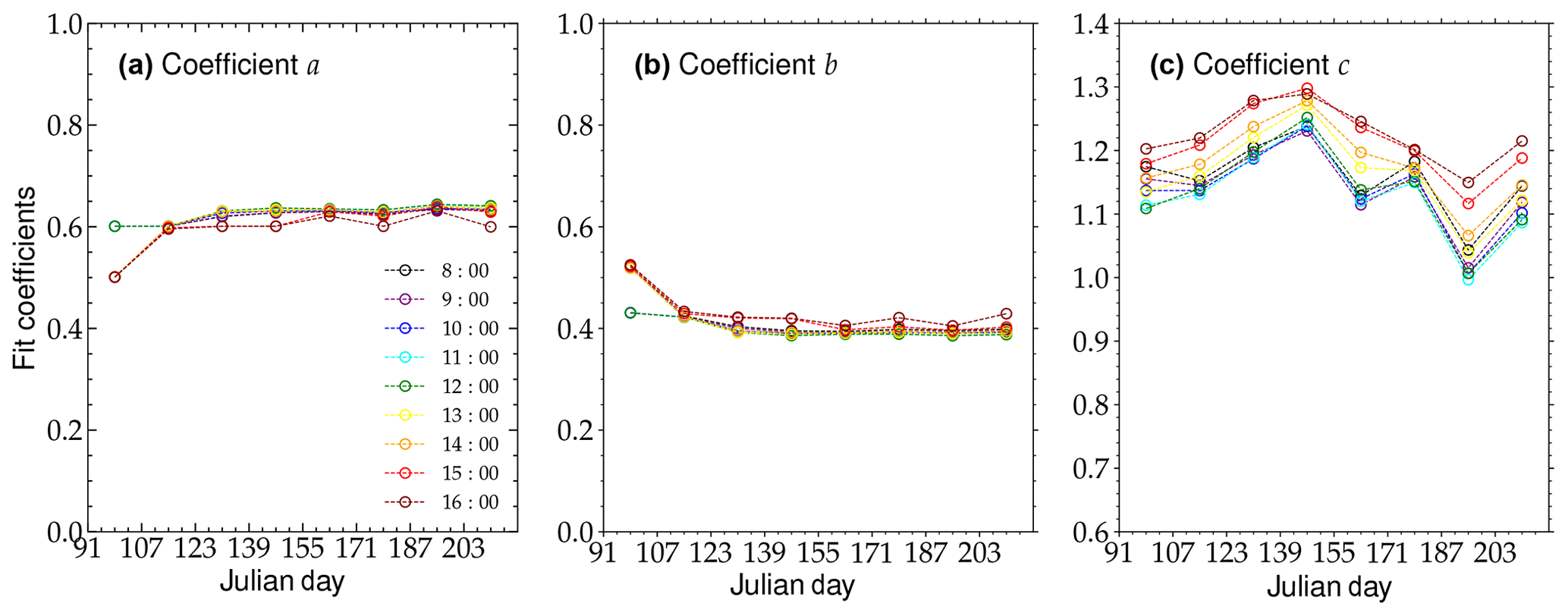
Figure 2(a) Fit coefficients a, which are used to derive higher-resolution SEVIRI reflectances by means of statistical downscaling, as a function of Julian day. Coefficients are derived hourly and in 16 d intervals for the Germany domain between 1 April and 31 July 2013. Colors illustrate different UTC times. (b) Same as (a) but for fit coefficients b. (c) Same as (a) but for fit coefficients c.
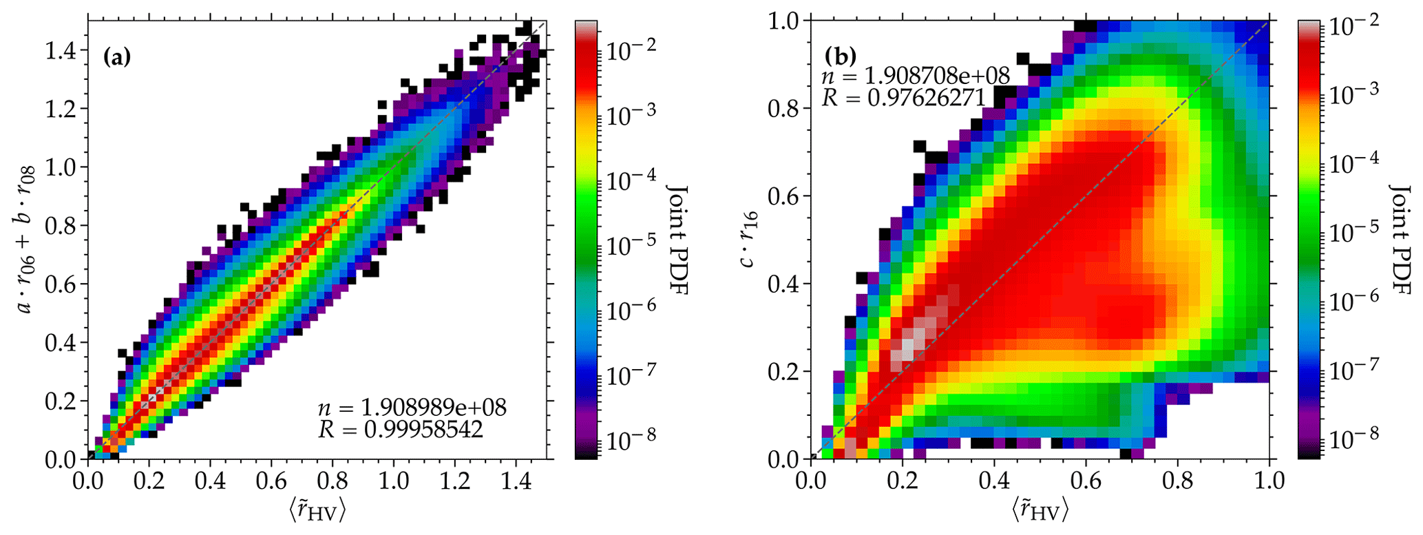
Figure 3(a) Joint probability density function (PDF) of smoothed SEVIRI HRV reflectances () and those obtained from a linear model of observed SEVIRI channel 1 (r06) and channel 2 (r08) reflectances, specifically (see Sect. 4.1). Data are from all 5 min SEVIRI observations of the Germany domain during June 2013. Only cloudy pixels are considered. The number of samples (n) and correlation coefficient (R) are given. (b) Same as (a) but for a linear model for SEVIRI SWIR reflectances, specifically c⋅r16.
Values of hourly derived fit coefficients for the Germany domain between 1 April and 31 July 2013 are shown in Fig. 2a and b for a and b, respectively. Here, circles represent the respective fit coefficient for each 16 d interval, which is indicated by the first Julian day in the time period. Colors highlight the different UTC time steps. It is obvious that both coefficients a and b are very stable and show no noticeable variation from hour to hour, as well as from one 16 d interval to another. Considering all hourly data and each 16 d interval, the median fit coefficients are 0.63 (for a) and 0.40 (for b), with low interquartile ranges (IQR) of 0.03. The only exceptions are the fit coefficients derived for the first time period of 1–17 April 2013, especially for the morning and afternoon hours of 08:00–09:00 and 13:00–16:00 UTC. Here, a and b deviate significantly from the other results, with values of ≈0.50 and ≈0.52, respectively, likely due to an abundance of observations with large solar zenith angles of in the eastern part of the domain.
The high-frequency reflectance variations for the SEVIRI HRV channel (δrHV) are calculated as the difference between the observed rHV and , which only resolve the low-frequency variability:
Following the linear model in Eq. (1), the high-frequency variations of the channel 1 and 2 reflectances (δr06 and δr08) are linked to δrHV via
The optimal slopes S06 and S08, which minimize the least-squares deviations, can be derived from bivariate statistics:
Here, cor(r06,r08) is the linear correlation coefficient between the channel 1 and 2 reflectances, while var(r06) and var(r08) are the spatial variances of the respective samples. Note that the sampling resolution of all reflectances is the LRES scale (i.e., ).
As a result, the high-resolution reflectances and , which include the high-frequency variations, can be derived from the interpolated reflectances as
Note that only is used for the retrieval.
Similar steps can be applied for the calculation of . Again, a simple linear model is assumed to connect r16 to the lower-resolution at the spatial scales of the channel 1–3 observations:
The symbol c is used to denote the respective fit coefficient, which needs to be determined empirically. Similar to the coefficients a and b from the linear model for the VNIR reflectances, c is calculated hourly between 08:00 and 16:00 UTC within 16 d intervals. It has to be noted, however, that in contrast to the VNIR reflectances this fit does not have a clear physical motivation, as there is no spectral overlap with the HRV channel.
The temporal behavior of the fit coefficient c for the Germany domain for the time period between 1 April and 31 July 2013 is shown in Fig. 2c. In contrast to the coefficients a and b, there is a noticeable trend in the data, both diurnally and during the transition from 1 April to 31 July. For each 16 d interval the variability in the hourly derived c values ranges between IQR=0.05 and 0.15, while the median 16 d value varies between 1.04 and 1.25. Overall, the median c is 1.16, with an IQR of 0.08 (i.e., almost 3 times larger than the one for the coefficients a and b). The observed trends and larger IQR in the c data set shown in Fig. 2c illustrate that the linear model in Eq. (6) is not ideal and is expected to introduce significant uncertainties in the calculation of . This behavior is expected, as the relationship between VNIR and SWIR reflectance can usually not be described by a linear function (see discussions in Werner et al., 2018a, b, as well as the LUT examples in Fig. 4 later in this study). For a constant reff there is a linear increase in r16 with increasing r06, as the cloud optical thickness increases. However, the slope of this linear relationship increases with decreasing reff. For τ>10 the relationship between r16 and r06 is characterized by a prominent curvature, while for τ≫10 the r16 values become independent of r06. Therefore, the fit coefficients c depend on the distribution of cloud optical and microphysical parameters, which varies widely with cloud type, meteorological conditions, and different dynamic processes.
Values of can be derived similarly to Eqs. (3–5) for the channel 1 and 2 observations:
Note that the use of linear models and bivariate statistics means that the downscaling algorithm described in this section is an example of statistical downscaling techniques, which are common in climate science applications (e.g., Benestad, 2011). While for the VNIR channels the spectral overlap with the HRV channel and the spectrally flat properties of clouds provide a sound physical justification for this technique, this is not the case for the SWIR channel.
The reliability of the linear model in Eq. (1) depends upon the correlation between channel 1 and 2 reflectances (i.e., cor(r06,r08)), as well as the stability of the fit coefficients a and b. The analysis in Deneke and Roebeling (2010) concludes that the explained variance in the estimates of and is close to 1, corresponding to low residual variances, which indicates that the linear model is robust. Moreover, the two fit coefficients are found to exhibit very low variability, as shown in Fig. 2a–b.
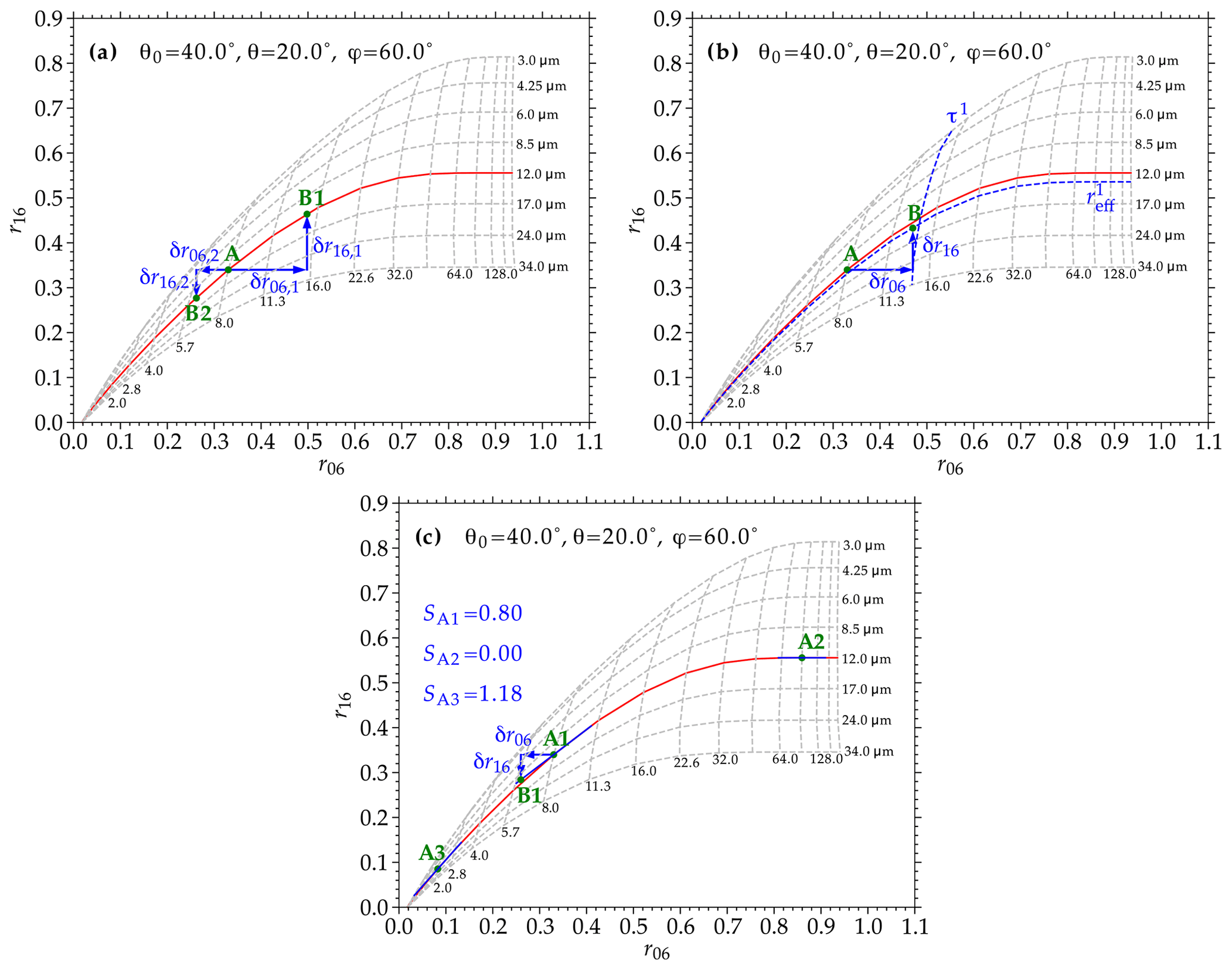
Figure 4(a) Example SEVIRI lookup table for liquid-phase clouds, illustrating the lookup table approach (introduced in Sect. 4.3) for an observation highlighted by the reflectance pair indicated by point A. For two different high-frequency variations of the channel 1 reflectance (δr06,1 and δr06,2) the derived high-frequency variations of the channel 3 reflectance (δr16,1 and δr16,2) are shown. See text for more description. (b) Same as (a) but illustrating the adjusted lookup table approach (introduced in Sect. 4.4) with the adiabatic adjustment for a single δr06 example. (c) Same as (b) but with the LUT slope adjustment.
To verify the reliability of the linear model with a large SEVIRI data set, a joint PDF of the actually observed and the results from Eq. (1) is shown in Fig. 3a; data are from all SEVIRI observations within the Germany domain during June 2013. In case of an ideal linear model, as well as a perfect correlation between the two reflectances, Eq. (1) would replicate the observations. Conversely, deviations from these assumptions will yield different results from the sampled SEVIRI reflectances. It is clear that the linear model can reliably reproduce , as most of the observations lie on the 1:1 line, and Pearson's product-moment correlation coefficient (R) is R=0.999. While some larger deviations exist, such occurrences are significantly less likely (i.e., the joint probability density is several orders of magnitude lower than the most-frequent occurrences along the 1:1 line). Regarding r16, the assumption of a linear model is evidently flawed, because the relationship between VNIR and SWIR reflectances depends on the optical and microphysical cloud properties. As a result, a single linear slope, which describes the whole relationship between the two reflectances for all distributions of cloud properties, will introduce significant uncertainties. This is illustrated in Fig. 3b, where the joint PDF of and the results from the linear model in Eq. (6) are shown. The comparison between the two data sets reveals a much larger spread around the 1:1 line and a lower correlation coefficient. Overall, the relationship resembles the shape of a LUT, displayed in the form of the well-known diagram introduced by Nakajima and King (1990), where changes in reff result in a spread in the observed SWIR reflectances (see, e.g., Werner et al., 2016).
To test the impact of changes in a and b on the derived and , two experiments are conducted: (i) the fit coefficients are derived only from cloudy pixels and are compared to the higher-resolution results from a and b, which are derived for all pixels; and (ii) the Germany domain is divided into 100 km×100 km subscenes, and the fit coefficients are derived more locally within each subscene instead of globally from the full domain. Subsequently, statistics from the difference between the two data sets are calculated. Data are from 14 June 2013 at 14:05 UTC. For experiment (i), the 1st, 50th, and 99th percentiles of the relative difference in (defined as the difference between the reflectances from only cloudy data and the full data set, normalized by the full data set) are −0.08, −0.02, and 0.03 %, while for the analysis yields −0.04, 0.02, and 0.19 %. Similarly, experiment (ii) yields relative differences of −0.08, 0.03, and 0.36 % and −0.17, 0.00, and 0.19 % for and , respectively. These deviations are negligible compared to the measurement uncertainty, and naturally the correlation coefficients between the different data sets are R≈1.00. This confirms the robustness of the linear model described in Eq. (1). For the derivation of from Eq. (6), a slightly increased sensitivity to the fit coefficient c is observed. Here, experiment (i) yields percentiles of the relative difference of −0.16, 0.08, and 0.86 %, whereas experiment (ii) results in −0.39, −0.01, and 0.40 %. While slightly higher deviations are observed compared to the linear model for the VNIR reflectances, the uncertainty in induced by the variability in c is still significantly lower than the measurement uncertainty.
4.2 Constant reflectance ratio approach
Compared to the downscaling approach in Sect. 4.1, where fit coefficients for a linear model are derived over a large temporal and spatial domain, this second method uses local relationships (i.e., on the pixel level) between the SEVIRI reflectances. The constant reflectance ratio approach was introduced by Werner et al. (2018b) and is based on the assumption that the inhomogeneity index of the HRV reflectance (Hσ,HV, defined as the ratio of standard deviation σHV to the average, pixel-level reflectance ) equals that for the channel 1 reflectance (Hσ,06). This implies a spectrally consistent subpixel reflectance variability. The relationship can be written as
where the index indicates any one of the nine available HRES subpixels within a lower-resolution SEVIRI pixel (i.e., at the LRES scale of channels 1–3). This relationship can be further simplified, assuming that this relationship is also true for individual pixels:
The relationship in Eq. (9) suggests that the ratio of channel 1 and HRV reflectances (i.e., narrowband and broadband VNIR reflectances) remains constant for different scales. Thus, this approach is called the constant reflectance ratio approach.
Finally, we can mitigate some of the scale effects by substituting the lower-resolution variables with the higher-resolution reflectances that resolve the low-frequency variability (i.e., and ) and solve for :
Similarly, higher-resolution SWIR reflectances can be derived from
As before, the relationship implies that the ratio of VNIR and SWIR reflectances remains constant for different scales. This assumption has been shown to be reasonable, at least for optically thin (i.e., τ≤10) liquid water clouds over the ocean (Werner et al., 2018b).
4.3 Lookup table approach
A third method to derive high-resolution cloud property retrievals for SEVIRI utilizes an iterative approach to determine δr06 and δr16 independently, based on the shape of the LUT, while constraining the observed reff to that of the baseline approach (i.e., simple trigonometric interpolation, which yields reflectances and that only resolve the large-scale variability). While the previous approaches can be implemented as a preprocessor outside the actual retrieval, this method requires access to the LUT and has thus been implemented through modifications of the CPP retrieval algorithm.
Again, a simple linear relationship between δrHV, δr06 and δr08 based on Eq. (2) is assumed:
where the fit coefficients a and b are determined from the same techniques as described in Sect. 4.1. The variation δrHV of the HRV channel is obtained from the observations following Eq. (2), while δr08 is calculated as the difference between r08 from high- and low-resolution optical thickness τ based on the functional relation ℱ of the reflectances and cloud properties stored in the LUT (which motivates the name of this method). Therefore, δr06 can be derived from
Note that the addition of δr08 in the calculation of δr06 helps to account for the noticeable increase in surface albedo of vegetation-like surfaces at λ>700 nm (i.e., the vegetational step). This should improve the estimation of δr06 for thin clouds (i.e., τ<10) and cloud-edge pixels. For the SWIR reflectance, instead of relying on the imperfect linear model in Eq. (6) or assumptions about the inhomogeneity index Hσ,16, the adjustment δr16 is determined iteratively to conserve the coarse-resolution, pixel-level (i.e., LRES scale of channels 1–3) value of the effective droplet radius. To reduce some of the associated uncertainties, the effective droplet radius based on the reflectances from triangular interpolation can be used instead of the LRES result. If and are the cloud properties based on trigonometric interpolation, and and are the higher-resolution retrievals, which are derived from an inversion of the functional relationship (ℱ) between the high-resolution reflectances and following
then δr16 can be determined as
This implies that a positive or negative δr06 is connected to a positive or negative δr16 using the LUT to adjust the SWIR subpixel reflectance variations in such a way as to be representative of the respective standard-resolution . As a result, we do not expect any improvement for the reff retrieval during the transition to smaller scales. Instead, we try to find a physically reasonable constraint for δr16 to achieve a reliable retrieval of the higher-resolution , while retaining the accuracy of the standard-resolution retrieval of .
The LUT approach is illustrated in Fig. 4a, where an example SEVIRI liquid-phase LUT for a specific solar zenith angle (), sensor zenith angle (), and relative azimuth angle () is shown. Vertical dashed lines and values below the grid denote fixed , while the horizontal dashed lines and values to the right of the grid denote fixed in units of micrometers. The green dot highlighted by the capital letter A represents an example SEVIRI reflectance pair of approximately and , which maps to and (i.e., the retrieval result for the high-resolution reflectances from trigonometric interpolation). The red line highlights the isoline. The two horizontal blue arrows indicate a positive (δr06,1) and negative (δr06,2) adjustment to based on Eq. (13). Without an adjustment to , these newly derived higher-resolution values map to significantly larger and lower effective droplet radii of about and , respectively. The adjustments δr16,1 and δr16,2 simply assure that the prior effective radius retrieval is preserved (i.e., ). Due to the curvature of the isolines of fixed given by the LUT, small deviations of the coarse-resolution average from can still occur.
Note that the LUT approach requires a prior cloud phase retrieval (either from the lower-resolution or interpolated reflectances) to determine the correct LUT for either liquid water or ice.
4.4 Adjusted lookup table approach
In order to improve the estimation of δr16 in the LUT approach, two modifications to the previous assumption are introduced in this section. The first one aims to provide a more realistic estimate of compared to the coarser LRES result, which subsequently is used to determine δr16. The value of is derived from adiabatic theory, which provides a physically sound relationship between the derived high-resolution cloud variables:
Based on observations, the study by Szczodrak et al. (2001) confirmed the value of a≈0.2 predicted by theory for marine stratocumulus, so this is the value also adopted here. This approach is illustrated in Fig. 4b, where the retrieval based on the interpolated reflectances at point A is indicated by the red reff isoline. During the first iteration step δr06 is derived from Eq. (13) and δr16=0, which maps to in the LUT (the exponent 1 indicates the first iteration step). This value is highlighted by the vertical blue line. Based on Eq. (16) the corresponding adiabatic is calculated (highlighted by the horizontal blue line). This value determines the adjustment δr16. Note that the resulting reflectances at point B do not exactly map to after the first iteration. As a result, multiple iterations are necessary to derive the final cloud properties. It has however been relatively simple to merge this iteration into the iterative retrieval loop of the CPP retrieval.
A second approach to improve upon the LUT approach again utilizes the shape of the LUT to derive a local slope from the simulated LUT reflectances. The value of S is calculated at the position denoted by and . In the iterative CPP retrieval, this requires that both low- and high-resolution cloud properties are estimated during each iteration until convergence of both properties is achieved. This approach is illustrated in Fig. 4c. Again, the initial retrieval based on the interpolated reflectances at point A1 is indicated by the red isoline. The slope SA1 at this position in the LUT is highlighted by the solid blue line. Based on the derived slope and δr06 from Eq. (13) the corresponding δr16 can be calculated for each iteration step. Two additional examples for initial starting points (A2 and A3) and the respective slopes (SA2 and SA3) are also shown. These examples indicate the change in slope for different parts of the LUT. For small , the slope SA3 become steeper, which leads to a larger adjustment δr16. Meanwhile, for large (for this specific viewing geometry and LUT) the and isolines are nearly orthogonal and both the respective slope SA2 and δr16 are close to 0.
Both approaches introduced in this section have advantages and disadvantages but promise to improve on the standard LUT approach. While physically sound, adiabatic assumptions might not always be appropriate, especially for highly convective clouds or in the presence of drizzle. Meanwhile, large δr06 adjustments might map to a point in the LUT where the derived local slopes at the position of and might not be representative anymore.
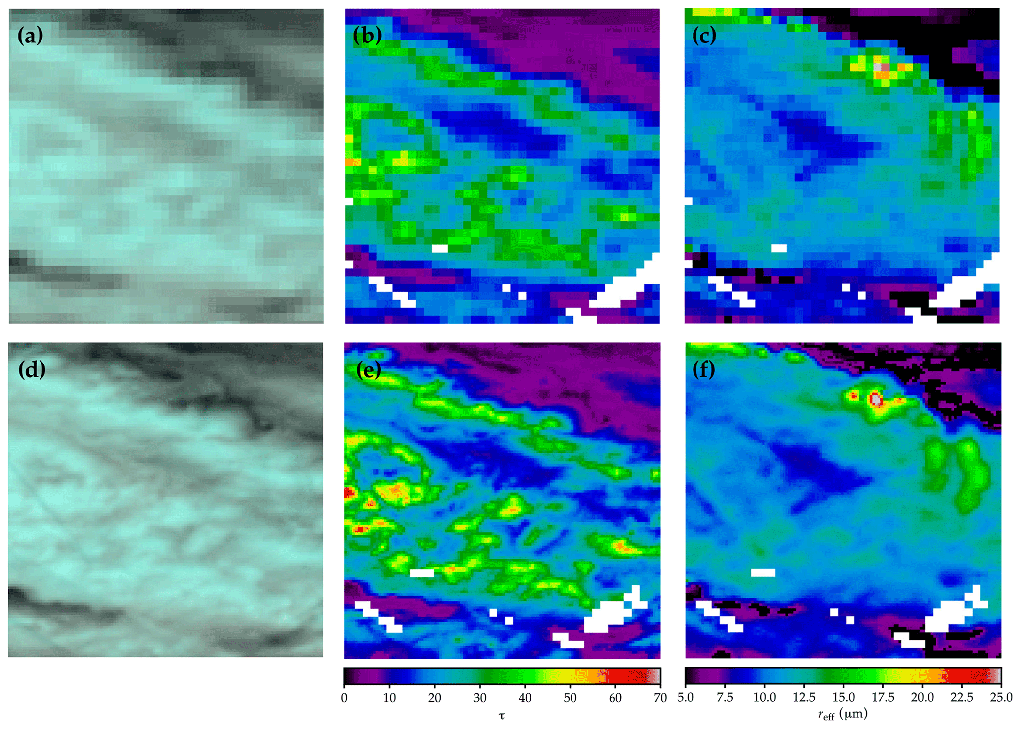
Figure 5(a) RGB composite image of SEVIRI channel 3, 2, and 1 reflectances at the instrument's native horizontal resolution of 3 km×3 km. Data are from a subregion within the Germany domain on 9 June 2013 at 10:55 UTC. (b) Similar to (a) but illustrating a map of the cloud optical thickness (τ). White colors indicate pixel with either a failed cloud property retrieval, a nonliquid cloud phase, or noncloud designation by the cloud masking algorithm. (c) Same as (b) but for the effective droplet radius (reff). (d)–(f) Same as (a)–(c) but at a horizontal resolution of 1 km×1 km. The reflectances and retrievals have been derived from the adjusted lookup table approach as described in Sect. 4.4, using the LUT slope adjustment.
An example of a standard SEVIRI red, green, and blue (RGB) composite and the respective cloud property retrievals, utilizing the native r06 and r16, are shown in Fig. 5a–c. In comparison, the retrieval results using the downscaled and from the adjusted lookup table approach, using the LUT slope adjustment, are presented in Fig. 5d–f for the same cloud field. The example is a subscene of SEVIRI observations of an altocumulus field, which was acquired on 9 June 2013 at 10:55 UTC over ocean within the Germany domain. The three illustrated parameters are an RGB composite image of SEVIRI channel 3, 2, and 1 reflectances in panels a and c; the cloud optical thickness τ and in panels b and e; and the effective droplet radius reff and in panels c and f. For the cloud variables only liquid-phase pixels are shown. An increase in contrast and resolved cloud structures is visible in the higher-resolution RGB composite. Regarding the retrieved cloud properties, the fields of lower-resolution τ and reff are a lot smoother, and the results exhibit a lower dynamical range than their higher-resolution counterparts. One obvious example is the bright cloudy part along 54.6∘ N, where τ>45 are observed. Moreover, the region of low reff in the northeastern corner of the scene exhibits more nuanced values in the higher-resolution data set.
This section presents an evaluation of the different downscaling techniques, which are introduced in Sect. 4, by means of MODIS observations. MODIS provides reflectances at a horizontal resolution of . These observations are remapped to the higher-resolution grid of the SEVIRI rHV-band samples, thus simulating a hypothetical SEVIRI-like geostationary instrument, where all channels are provided at the HRES scale. This provides the means to derive reference retrievals of τ and reff. Note that even though these reference retrievals are performed at a higher resolution the “” notation is omitted, because these cloud products are derived from actual observations and are not the estimates obtained from the various downscaling techniques.
Remapping MODIS reflectances to SEVIRI's LRES grid (i.e., the native resolution of channels 1–3) subsequently provides the means to apply the various downscaling schemes, as well as the simple triangular interpolation approach, in order to compare the retrieved cloud products (i.e., and , as well as and ) to the reference results. Naturally, the ideal downscaling approach would yield results that closely resemble the MODIS-provided HRES observations. Furthermore, the ideal downscaling approach would also represent an improvement upon the simple interpolation technique. The reader is reminded that the latter data are still available at a higher resolution than the native LRES grid of the SEVIRI r06, r08, and r16 channels but no longer contain any information about the high-frequency reflectance variability. As the simplest approach to derive higher-resolution cloud products, these results are called the baseline results.
In addition, a comparison can be made to those cloud variables, which would be obtained from reflectances at SEVIRI's native spatial resolution by setting each 3×3 HRES pixel block to the LRES value.

Figure 6(a) RGB composite image of remapped MODIS channel 6, 2, and 1 reflectances at the horizontal resolution of SEVIRI's HRV channel at a horizontal scale of 1 km×1 km at the subsatellite point. Data are from example scene 1 sampled on 1 June 2013 at 10:05 UTC. (b)–(d) Same as (a) but for example scenes 2 to 4, sampled on 9, 6, and 5 June 2013 at 10:55, 11:20, and 10:25 UTC, respectively.
Figure 6 shows RGB composites of the four example scenes, which comprise the data set for the evaluation of the different downscaling techniques. The scenes are increasingly more heterogeneous, starting with a rather homogeneous altocumulus field in Fig. 6a, two more heterogeneous broken altocumulus examples in Fig. 6b–c, and finally a broken cumulus field in Fig. 6d.
Table 1Description for the different retrieval experiments, which are characterized by different assumptions for the downscaling of SEVIRI reflectances from the native horizontal resolution of ≈3 km to the MODIS-like ≈1 km scale.
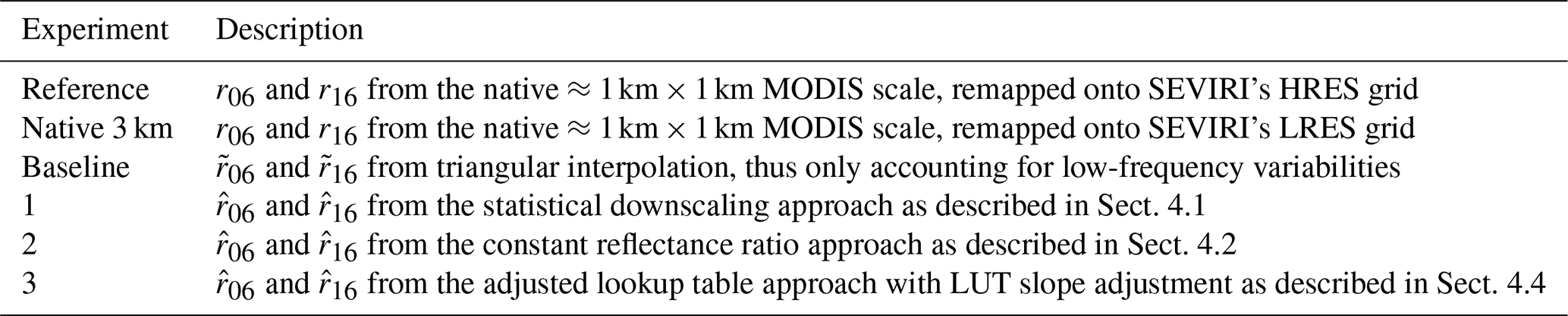
Meanwhile, Table 1 summarizes the different retrieval experiments that form the comparison in this section. For the sake of completeness, the reference data (i.e., the results from the MODIS reflectances, which are remapped to SEVIRI's HRES grid) are also included. Retrievals based on remapped MODIS data to SEVIRI's native 3 km scale are reproduced to each of the 3×3 subpixels to match the horizontal resolution of the reference results. Meanwhile, the cloud products derived from triangular interpolation of the remapped LRES–MODIS samples are referred to as the baseline data set, as this is the easiest approach and any reliable downscaling technique needs to add an improvement on those results. Experiment 1 denotes the statistical downscaling approach from Sect. 4.1, while retrievals based on the constant reflectance ratio approach and the adjusted LUT approach with LUT slope adjustment are indicated as experiments 2 and 3, respectively. Note that we also performed analysis for the standard LUT approach, as well as the adjusted LUT approach with adiabatic adjustment. However, we will only briefly summarize the results of these downscaling schemes where necessary.
First, the collocation and remapping procedure for the native MODIS reflectances is briefly described. A comparison between the retrieved cloud products from the LRES resolution–reflectances and those from triangular interpolation, as well as the different downscaling procedures, and the reference results follows in Sect. 6.2. These retrievals can be used to derive estimates of the liquid water content (WL, , and ) and the droplet number concentration (ND, , and ), which are evaluated in Sect. 6.3.
6.1 Reprojection of MODIS swath radiances to the SEVIRI grid
To obtain a reliable higher-resolution reference data set, MODIS level 1b swath observations (MOD021km) have been projected to the grid of SEVIRI's rHV samples, which corresponds to the geostationary satellite projection at the HRES scale. Initially, the native HRV grid is oversampled by a factor of 3 in each dimension (i.e., the target grid has a ≈333 m resolution), and nearest-neighbor interpolation is used for the projection. This oversampled field is subsequently smoothed with the modulation transfer function of the HRV channel as given by EUMETSAT (2006), to remove high-frequency variability not resolved by the sensor and, in particular, the artifacts introduced by the nearest-neighbor interpolation technique. Finally, this field is downsampled, such that only each central pixel of a 3×3 block (each pixel with a horizontal resolution of 333 m) is retained to represent the HRES value.
To perform the subsequent downscaling experiments, a second set of level 1b radiances are generated, where the spatial variability is reduced to match that of the LRES channels of Meteosat SEVIRI. This step again involves the smoothing of the respective reflectance field with the channel-specific modulation transfer function of the lower-resolution SEVIRI channels (EUMETSAT, 2006). This data set represents hypothetical SEVIRI-like observations at the native LRES.
In addition, a band-pass filter has been constructed from the difference between the modulation transfer functions of the HRV and the 0.6 and 0.8 µm channels (weighted by the coefficients of a linear model; see Deneke and Roebeling, 2010). This filter is used to extract the high-frequency signal of the HRV channel.
It should be noted that retrievals based upon these radiances will be different than those based upon the original MODIS C6 radiances or from an absolutely accurate representation of the (hypothetical) truly observed, high-resolution SEVIRI samples. For one, it uses the linear model of Cros et al. (2006) and Deneke and Roebeling (2010) as a proxy for the HRV channel, thereby excluding a potentially significant source of uncertainty. Moreover, MODIS acquires these reflectances under different viewing geometries (note that the true viewing angles are used in the CPP retrieval, so within the limits of plane-parallel radiative transfer, this effect is accounted for), and the spectral characteristics of the MODIS and SEVIRI channels are not entirely comparable. However, the goal of this study is to provide a consistent reference data set for a comparison of different retrieval data sets, which are derived from a single retrieval algorithm core. The actual absolute values of the retrieved cloud products are not important here.
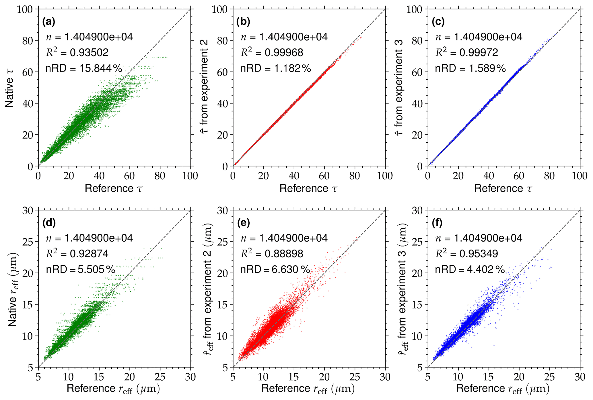
Figure 7(a) Retrieved cloud optical thickness (τ) at SEVIRI's native LRES as a function of the reference results (τ derived from the remapped MODIS reflectances at the HRES scale of ≈1 km). Data are from example scene 2, sampled on 9 June 2013 at 10:55 UTC. The dashed gray line represents the 1:1 line. The number of samples (n), explained variance (R2), and normalized root-mean-square deviation (nRD; defined as the RD between the two data sets, normalized by the average reference τ) are given. (b)–(c) Same as (a) but for the comparison between τ and the downscaling results () from experiments 2 (constant reflectance ratio approach) and 3 (adjusted lookup table approach with LUT slope adjustment), respectively. (d)–(f) Same as (a)–(c) but for the effective droplet radius (reff and ).
6.2 Results for τ and reff
Figure 7a shows a comparison of τ at the native LRES (replicated onto each subpixel) and the reference τ at the HRES scale for the example cloud field in scene 2, which is shown as an RGB composite image in Fig. 6b. A total of over 13 000 cloudy pixels (liquid phase) are located in this scene. While for small reference τ<20 there is a reasonable agreement between the two data sets, there is increased scatter around the 1:1 line (indicated by the dashed gray line) for larger values of cloud optical thickness. For reference τ>40, a substantial underestimation of the LRES τ is observed, which yields a sizable contribution to the nRD of 15.8 %. Figure 7b–c show similar scatter plots of τ and from both experiment 2 (constant reflectance ratio approach) and 3 (adjusted LUT approach with LUT slope adjustment), respectively. It is obvious that the results from these two downscaling techniques improve the agreement with the reference retrievals significantly. The explained variance (R2, which equals the square of Pearson's product-moment correlation coefficient R) between the data sets is increased, and the nRD is strongly reduced to values of 1.182 % (experiment 2) and 1.589 % (experiment 3).
A similar comparison between the reference reff at the HRES scale and reff at native LRES, as well as from the same downscaling experiments, is presented in Fig. 7d–f. Here, the native-resolution results show a much better agreement with the reference retrievals, and, compared to the cloud optical thickness, the nRD=5.505 % is much lower. While experiment 2 exhibits a good agreement between reference τ and , the comparison of retrieved to the reference results is less favorable. Both the reduced explained variance (R2=0.889 versus R2=0.929) and the increased scatter around the 1:1 line (nRD =6.630 %) indicate that the results from experiment 2 are less reliable than the ones performed at the native LRES. Thus, the elaborate downscaling procedure actually reduces the accuracy of the retrieval. In contrast, the retrieved values from experiment 3 improve upon the native-resolution results, with slightly better values of R2=0.953 and nRD =4.402 %.
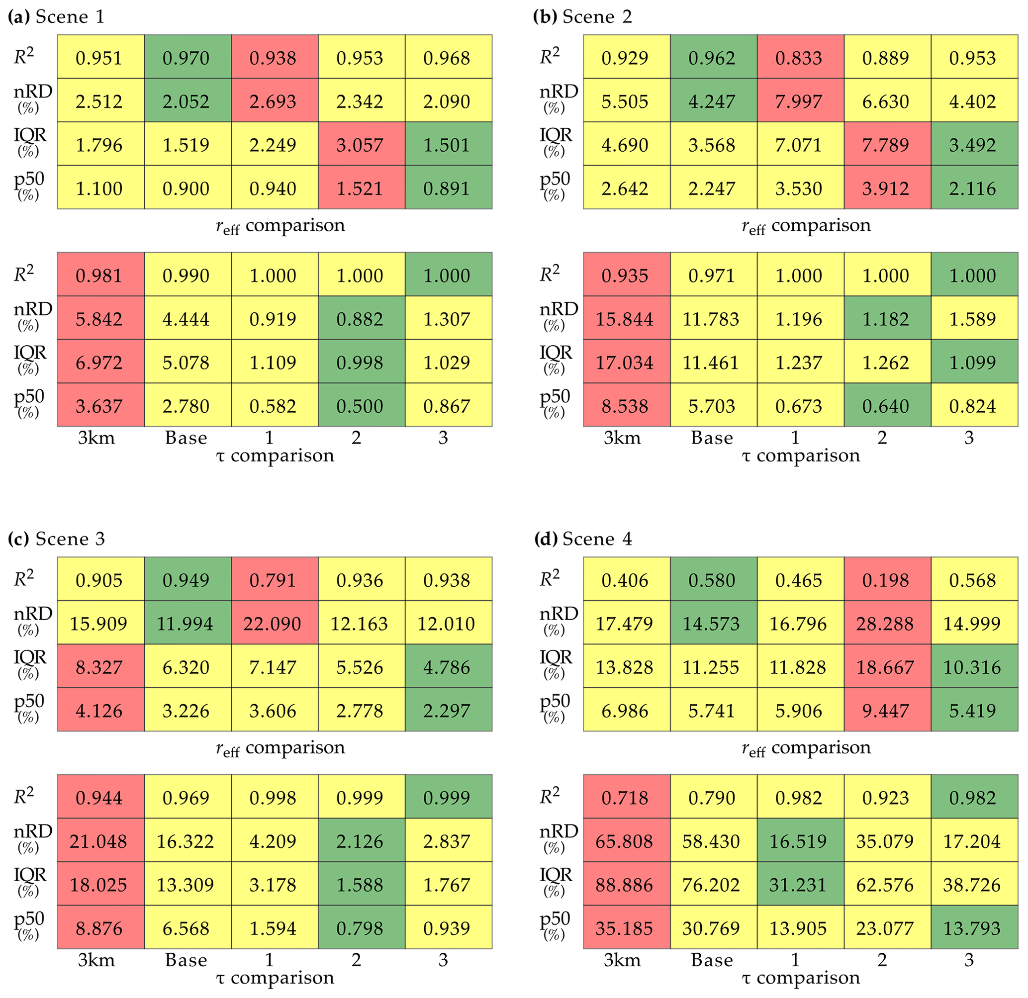
Figure 8(a) Comparison of retrieved cloud optical thickness (τ, c, d) and effective droplet radius (reff, a, b) from the native LRES (at a scale of ≈3 km) and baseline retrievals (i.e., only accounting for low-resolution reflectance variability), as well as the downscaling experiments 1 (statistical downscaling approach), 2 (constant reflectance ratio approach), and 3 (adjusted lookup table approach with LUT slope adjustment), and the reference retrieval results. Parameters to quantify the comparisons are the median of the relative difference to the reference (p50), relative interquartile range (IQR; 75th–25th percentile of the relative difference to the reference), normalized root-mean-square deviation (nRD; defined as the RD between the two data sets, normalized by the average reference retrieval), and the explained variance (R2). Green colors indicate the experiment that compares best to the reference results, i.e., highest R2 and lowest p50, IQR, and nRD. Red colors indicate the experiment with the worst agreement with the reference retrievals, while yellow colors indicate all experiments in between. Data are from example scene 1 sampled on 1 June 2013 at 10:05 UTC. (b)–(d) Same as (a) but for example scene 2 to 4, respectively.
Statistics of the comparison between the reference and native LRES, baseline, and experimental retrievals are presented in Fig. 8a–d for example scenes 1–4, respectively. The parameters which are used to quantify the individual comparisons are the median of the relative difference (abbreviated with p50) to indicate the average deviation from the reference results, the interquartile range (IQR; defined as the relative difference between the 75th and 25th percentile of the deviation to the reference retrievals) to indicate the spread between the different data sets, the nRD as a second measure of the spread of data points, and the explained variance R2 between the different retrievals and the reference. Values with a green and red background highlight the respective experiment with the best and worst comparison for the specific parameter. Yellow backgrounds, meanwhile, indicate all other experiments in between the two extreme results. The first noteworthy observation concerns the native and baseline retrievals of τ, which universally exhibit the largest median deviations and spread to the reference results, as well as the lowest R2. Still, the difference between native and baseline results indicates that the trigonometric interpolation to the HRES grid has significantly improved the comparison.
In contrast, each retrieval of that accounts for small-scale reflectance variability yields significant improvements, regardless of the approach. This is especially obvious in the parameters that characterize the spread in the deviations, i.e., IQR and nRD, which are between 2–9 and 2–10 smaller for the various experiments and example scenes, respectively. Experiments 2 and 3 seem to achieve the best agreement with the reference retrievals.
Regarding the effective droplet radius, the agreement between the native LRES and (i) baseline retrievals and (ii) the reference results is significantly better. It is worth pointing out that, similar to the optical thickness comparison, the retrieval based on interpolating reflectances to the HRES grid performs better than the native-resolution reff retrieval for all scenes. The most reliable downscaling approach seems to be experiment 3, which performs noticeably better than experiments 1 (note the increased nRD and reduced R2 for scene 3) and 2 (increased spread and overall issues for the heterogeneous cloud field in scene 4). This indicates that the linear model in Eq. (6) or assumptions about a constant ratio of VNIR and SWIR reflectances are not adequate to estimate higher-resolution , at least not for certain cloud conditions. In the case of experiment 2 this is understandable, because the technique was developed for partially cloudy pixels (Werner et al., 2018b). These observations are characterized by a low cloud optical thickness, where the relationship between VNIR and SWIR reflectance can reliably be considered to be linear (see example LUTs in Fig. 4).
There is a notably better performance of experiment 3, the adjusted LUT approach with LUT slope adjustment, compared to the standard LUT approach highlighted in Sect. 4.3. Of particular note is the retrieval based on the standard LUT scheme, which compares significantly worse to the reference results (R2 of 0.890, 0.648, 0.751, and 0.581 for cloud scenes 1–4, respectively). This is somewhat surprising, because the specified goal of the standard LUT approach is to maintain the accuracy of the baseline retrieval, which has not been fully reached. We believe that this might be caused by the sensitivity of the cloud property retrieval to small reflectance perturbations, in particular for broken clouds. It is also an indication that assuming constant subpixel reff values within each LRES pixel is not sufficient. We plan to investigate this effect further in future studies. However, the second adjusted LUT approach, which determines SWIR reflectance adjustments based on adiabatic theory, performs even worse (R2 of 0.846, 0.579, 0.741, and 0.519 for cloud scenes 1–4, respectively). This suggests that the observed cloud fields do not follow adiabatic theory and the method is not adequate to estimate higher-resolution .
6.3 Results for WL and ND
Retrievals of τ and reff (regardless of the resolution they are derived at) provide the means to infer other commonly used cloud variables. The WL, which describes the amount of liquid water in a remotely sensed cloud column, can be derived as the product of retrieved cloud products (Brenguier et al., 2000; Miller et al., 2016):
Here, ρL is the bulk density of liquid water. Assuming adiabatic clouds, where the vertical structure of effective droplet radius follows the adiabatic growth model, introduces an extra factor of 5∕6 and the coefficient 2∕3 changes to . Meanwhile, ND describes the number of liquid cloud droplets in a cubic centimeter of cloudy air. Calculating ND from remote sensing products requires a number of assumptions, e.g., about the vertical cloud structure and shape of the droplet number size distribution, which are summarized and discussed in Brenguier et al. (2000), Schüller et al. (2005), Bennartz (2007), and Grosvenor et al. (2018). A simplified form of the resulting equation for ND is
with (see Quaas et al., 2006). Note that Eqs. (17)–(18) can yield both baseline and downscaled results (i.e., and , as well as and ) when they are derived from the respective cloud optical thicknesses and effective droplet radii.
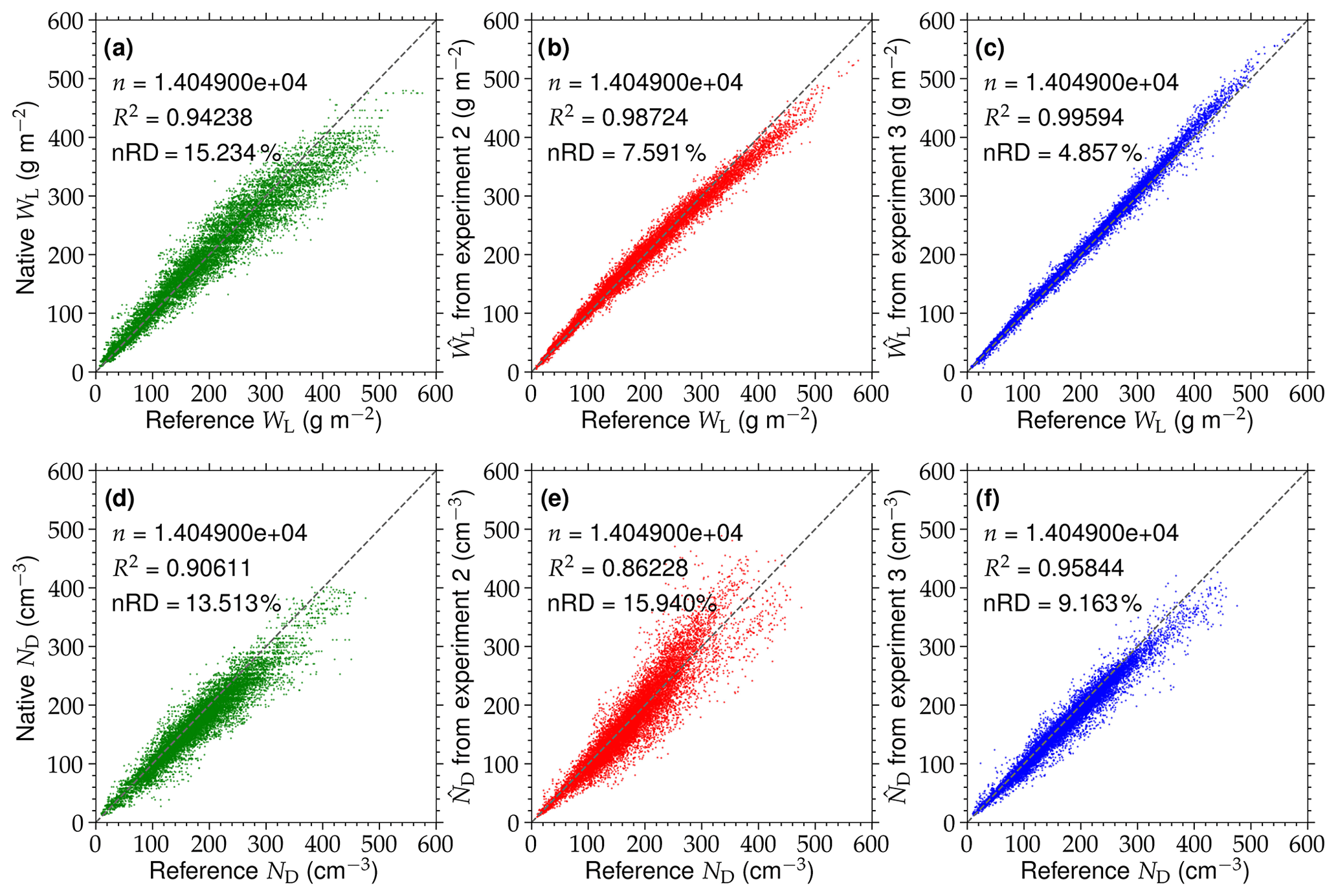
Figure 9(a) Retrieved liquid water path (WL) at SEVIRI's native LRES as a function of the reference results (WL derived from the remapped MODIS reflectances at the HRES scale of ≈1 km). Data are from example scene 2, sampled on 9 June 2013 at 10:55 UTC. The dashed gray line represents the 1:1 line. The number of samples (n), explained variance (R2), and normalized root-mean-square deviation (nRD; defined as the RD between the two data sets, normalized by the average reference WL) are given. (b)–(c) Same as (a) but for the comparison between reference WL and the downscaling results () from experiments 2 (constant reflectance ratio approach) and 3 (adjusted lookup table approach with LUT slope adjustment), respectively. (d)–(f) Same as (a)–(c) but for the droplet number concentration (ND and ).
Similar to the comparison in Sect. 6.2, scatterplots of the reference WL, the native LRES WL, and the results from the downscaling experiments 2 and 3 () are shown in Fig. 9a–c, respectively. As before, data are provided by example scene 2 sampled on 9 June 2013 at 10:55 UTC. Compared to the native LRES results, a noticeable improvement in the correlation and nRD is achieved by utilizing the two downscaling experiments. Not only are retrieved values closer to the 1:1 line, but the significant underestimation of the LRES WL values for larger reference results is mitigated. Especially for experiment 3, the spread is less than one-third of the value of the LRES results (4.857 % versus 15.234 %). Regarding the comparison between reference and native ND, as well as , downscaling experiment 2 yields less favorable results. There is a slight decrease (increase) in R2 (nRD). This is caused by the large IQR and nRD of the deviations in the retrieved , shown in Fig. 7e, which are amplified due to the associated power of 2.5 in Eq. (18). However, the derived values from experiment 3 show a significantly better agreement with the reference ND.

Figure 10(a) Comparison of derived liquid water path (WL, c, d) and droplet number concentration (ND, a, b) from the native LRES (at a scale of ≈3 km) and baseline retrievals, as well as the downscaling experiments 1 (statistical downscaling approach), 2 (constant reflectance ratio approach), and 3 (adjusted lookup table approach with LUT slope adjustment), and the respective reference results. Parameters to quantify the comparisons are the median of the relative difference to the reference (p50), relative interquartile range (IQR; 75th–25th percentile of the relative difference to the reference), normalized root-mean-square deviation (nRD; defined as the RD between the two data sets, normalized by the average reference retrieval), and the explained variance (R2). Green colors indicate the experiment that compares best to the reference results, i.e., highest R2 and lowest p50, IQR, and nRD. Red colors indicate the experiment with the worst agreement with the reference retrievals, while yellow colors indicate all experiments in between. Data are from example scene 1 sampled on 1 June 2013 at 10:05 UTC. (b)–(d) Same as (a) but for example scenes 2 to 4, respectively.
Values of p50, IQR, nRD, and R2 for the WL and ND comparison from the four example scenes are illustrated in Fig. 10a–d. Due to the large deviations between the native τ and the reference retrievals, WL values for the LRES results almost universally show the largest deviations to the reference values and thus the largest IQR and nRD, as well as the lowest explained variance. The exception is the heterogeneous cloud field in the fourth example scene, where the large deviations between from experiment 2 and the reference retrievals yield the worst comparison for the respective . The estimates based on the adjusted lookup table approach using the LUT slope adjustment (i.e., experiment 3) almost universally exhibit the best agreement with the reference results of WL.
Overall, 27 of the 32 comparisons (four cloud scenes, two cloud variables, and four statistical measures) exhibit the best performance for experiment 3. For the example scenes considered in this analysis, it is obvious that the adjusted lookup table approach with LUT slope adjustment is preferable to the other downscaling techniques and yields more reliable high-resolution cloud variables than the standard LRES results.
As before, we also tested the standard LUT approach highlighted in Sect. 4.3, as well as the second adjusted LUT approach, which determines SWIR reflectance adjustments based on adiabatic theory. Due to the poor performance of the retrieval, the results based on adiabatic assumptions show a similarly poor agreement with the reference results. Meanwhile, the cloud variables based on the standard LUT approach never show the best or worst performance but are almost universally worse than the adjusted lookup table approach with LUT slope adjustment. This again illustrates that assumptions of adiabatic clouds and constant subpixel reff values within each LRES pixel are not suitable for the cloud scenes analyzed in this study.
Apart from the constant reflectance ratio approach, the downscaling of r06 for each of the techniques presented in Sect. 4 uses the well-established relationship between r06, r08, and the averaged (see Fig. 3 and the discussion in Deneke and Roebeling, 2010). In contrast, downscaling of r16 is based on different assumptions about the microphysical structure and cloud heterogeneity, which induces a level of uncertainty in the subsequent cloud property retrievals. To test whether assumptions about r16 actually improve the retrieval of and , this section presents retrievals that include the results from the adjusted lookup table approach with LUT slope adjustment (i.e., experiment 3) for but do not include the respective downscaling schemes for . Instead, the SWIR reflectance for each sample is provided by the value derived from trigonometric interpolation.
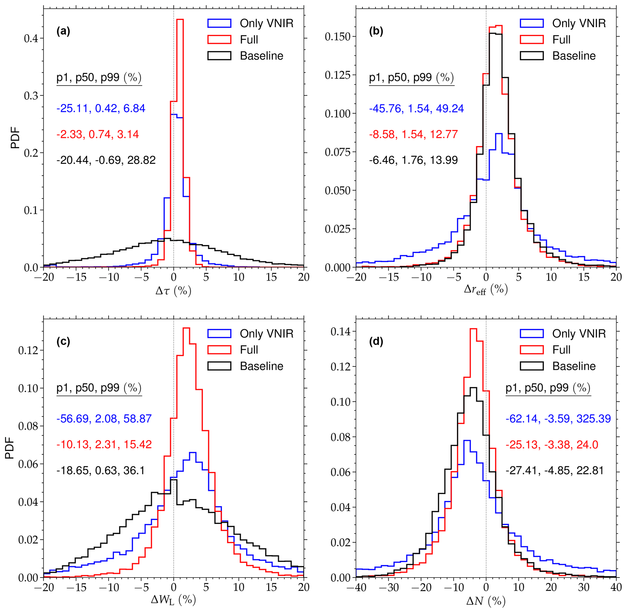
Figure 11(a) PDFs of the relative differences (Δτ) between the retrieved cloud optical thickness (τ) from the baseline test (black), as well as a VNIR-only and full downscaling approach for experiment 3 (shown in blue and red color, respectively), and the reference results (i.e., the original 1 km retrievals). Data are from example scene 2 sampled on 9 June 2013 at 10:55 UTC, which is shown in Fig. 6b. The 1st, 50th, and 99th percentiles of Δτ for each experiment are given. (b) Same as (a) but for Δreff, which is the relative difference for the retrieved effective droplet radius (reff). (c) Same as (a) but for ΔWL, which is the relative difference for the derived liquid water path (WL). (d) Same as (a) but for ΔND, which is the relative difference for the derived droplet number concentration (ND).
Figure 11a shows PDFs of the relative difference (Δτ) between from the baseline test (black), as well as retrieved from the partial downscaling approach of only (blue) and the full downscaling approach (red), and the reference results (i.e., distributions of the difference between the data sets, normalized by the reference τ). Data are from example scene 2, shown in Fig. 6b, sampled on 9 June 2013 at 10:55 UTC. The largest differences to the reference retrievals are observed for the baseline results, which only account for the large-scale reflectance variability of the cloud scene. Here, relative differences cover the range of (these values indicate the 1st and 99th percentile of Δτ, respectively). The distributions for the full downscaling experiment 3 are noticeably thinner, and these observed ranges are reduced significantly to . The differences Δτ for the VNIR-only approach look closer to the one from the full downscaling experiment. However, the maximum of the distribution around Δτ≈0 is lower and the 1st percentile is actually higher than that from the baseline retrievals. Clearly, the downscaling of both VNIR and SWIR reflectances is preferable for the retrieval of . For the effective droplet radius, the experiment comparison looks significantly different. Both relative differences Δreff based on the baseline and full downscaling experiment results exhibit a similar behavior, and the full downscaling approach only yields small improvements on the retrievals from trigonometric interpolation. Conversely, Δreff from partial downscaling yields a noticeably larger spread and the retrievals become less reliable.
Regarding ΔWL and ΔND, the results using the complete downscaling approach yield the narrowest distributions, with significantly smaller minimum and maximum deviations (up to a factor of 5.6) compared to the VNIR-only technique. Compared to the baseline results the reliability of derived liquid water path is also improved, even though just the VNIR reflectance is downscaled.
Table 2Comparison of the cloud property retrieval results from downscaling experiments 1–3, which only account for the VNIR part, and the full downscaling experiments, which include adjustments to both VNIR and SWIR reflectances. The comparison shows the 1st, 50th, and 99th percentiles of the relative differences Δτ (for the cloud optical thickness τ) and Δreff (for the effective droplet radius reff), which illustrate the deviation of the different retrieval approaches from the reference results, normalized by the reference retrievals. Data are from the four example scenes shown in Fig. 6.
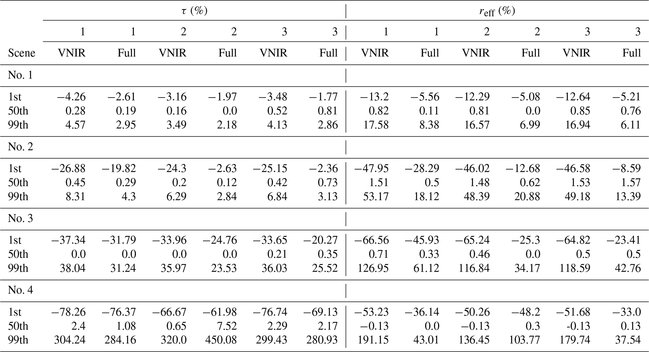
A summary of the performance of the partial and full downscaling approach for experiments 1–3 for all four example cloud scenes is given in Table 2. Here, the 1st, 50th, and 99th percentiles of the relative differences between and and the reference retrievals are listed. An almost universal reduction in the biases is observed when both VNIR and SWIR reflectances are downscaled. These results provide strong evidence that simultaneous downscaling of the SWIR reflectances is essential for providing reliable higher-resolution retrievals of and , as well as the subsequently calculated and . This confirms the findings in Werner et al. (2018b), who illustrated that SWIR reflectances differ significantly between the pixel level and subpixel scale and that reliable cloud property retrievals should avoid scale mismatches between the reflectances from the VNIR and SWIR channels.
This result is likely also relevant for retrieving cloud properties at the highest-possible resolution from other multiresolution sensors such as MODIS, VIIRS, and GOES-R: here, VNIR reflectances are generally available at the highest spatial resolution, while SWIR reflectances have a 2–4-times-lower sampling resolution. Based on the previous results, smooth interpolation of the SWIR reflectances to the VNIR resolution cannot be recommended. Instead, downscaling approaches such as those presented in Sect. 4 should be adopted to avoid a scale mismatch in the spatial variability captured by the VNIR and SWIR channels or, equivalently, a degraded accuracy of the reff retrieval.
In this work, several candidate approaches to downscale SEVIRI channel 1–3 reflectances are evaluated, which increases their spatial resolution from the native horizontal resolution (3 km×3 km at the subsatellite point) to the 3-times-higher spatial resolution of the narrowband HRV channel observations. The goal is to identify a reliable downscaling approach to provide the means to resolve higher-resolution, subpixel reflectance and cloud property variations, which are only resolved by reflectances from SEVIRI's coincident HRV channel. The higher-resolution reflectances are subsequently used to retrieve cloud optical thickness () and effective droplet radius (). These subsequently provide the means to derive estimates of the liquid water path () and droplet number concentration ().
Three different methods are presented and evaluated: (i) a statistical downscaling approach using globally determined fit coefficients based on bivariate statistics; (ii) a local approach that assumes a constant heterogeneity index for different scales (i.e., the constant reflectance ratio approach); and (iii) an iterative approach utilizing both global statistics and the shape of the SEVIRI LUT (which consists of simulated SEVIRI reflectances for different viewing geometries and combinations of cloud properties), while assuming a constant subpixel (i.e., the LUT approach). For the latter technique, two modifications (by assuming adiabatic cloud conditions or by deriving local slopes within the LUT) are introduced, which avoid the constraint of a fixed . The different downscaling approaches are evaluated using MODIS observations of four example cloud fields at a horizontal resolution of (i.e., comparable to SEVIRI's HRV channel), which are remapped onto the higher-resolution SEVIRI grid, followed by smoothing with the modulation transfer functions of SEVIRI.This approach has the benefit of providing a reference data set to which the results from the different downscaling techniques can be objectively compared.
The retrievals based on native-resolution reflectances (at a scale of ≈3 km) are characterized by significant deviations from the reference retrievals, especially for and . Here, random absolute deviations as large as ≈14 and ≈89 g m−2 are observed, respectively (determined from the 1st or 99th percentiles of the absolute deviations between native and reference results for each cloud scene). For and deviations of up to ≈6 µm and exist, respectively.
Simply applying trigonometric interpolation of the reflectance to the higher-resolution grid of the HRV channel (i.e., the baseline approach) provides a significantly improved agreement with the reference data set for τ and reff (i.e., the actual higher-resolution retrievals) compared to SEVIRI's native lower-resolution results. This improvement can be attributed to the use of higher-resolution reflectances, which resolve the large-scale variability of the scene. It is shown that either downscaling approach, which applies estimates of the unresolved small-scale variability to the reflectance field, yields reliable retrievals of at the horizontal resolution of the SEVIRI HRV channel. These results compare noticeably better with the reference retrievals than the ones from the baseline approach. The improved performance is illustrated by a lower median absolute bias and spread (factor of 2–10), as well as a higher observed correlation between the data sets. The reliability of utilizing the LUT approach with an adjustment based on the calculation of isoline slopes in the SEVIRI LUT is comparable to the baseline results and improves upon the retrievals at the native LRES. The performance of the other downscaling approaches depends on the observed cloud scene. For more heterogeneous cloud fields the performance of the statistical downscaling approach and the constant reflectance ratio approach decreases noticeably. The former technique relies on large-scale statistical relationships between the reflectances, which might vary with the size of the observed region, prevalence of different cloud types, and viewing geometry. The latter technique, meanwhile, was developed for optically thin clouds, where the relationship between VNIR and SWIR reflectance can be approximated by a linear function (Werner et al., 2018b). Conversely, for more homogeneous altocumulus fields the LUT approach with adiabatic adjustment seems inadequate and yields the worst comparison to the reference effective radius. The study by Miller et al. (2016), following similar studies, illustrated that drizzle and cloud top entrainment yield vertical cloud profiles closer to homogeneous assumptions and away from the adiabatic cloud model. Similar processes might affect the retrieval for the presented cloud scenes in this study.
Due to the fact that these variables are derived from retrieved and , a similar behavior is observed for the derived and . Again, the adjusted LUT approach in combination with the use of local slopes exhibits the best agreement with the reference results for 27 out of the 32 comparisons (i.e., four example scenes, two cloud variables, and four evaluation parameters). Based on these results, this method seems to be favorable compared to the other downscaling approaches. The results are preferable to those obtained from the standard-resolution SEVIRI narrowband reflectances and pave the way for future higher-resolution cloud products by the MSG-SEVIRI imager. Especially for and , these improvements are significant, as even the baseline results show deviations from the reference data set of up to ≈11 and for the observed example scenes.
Most of the presented downscaling techniques utilize a well-established relationship between the observed reflectance from SEVIRI channels 1 and 2, as well as the one from the broadband HRV channel. To test the validity of the different assumptions for the downscaling of the SWIR band reflectance, the reliability of VNIR-only downscaling approaches is compared to the corresponding full downscaling procedure. For the former, the higher-resolution SWIR observations are provided by the baseline technique. An almost universally improved reliability of the retrieved cloud products is observed when both VNIR and SWIR reflectances are downscaled. This illustrates that, in order to achieve reliable higher-resolution retrievals, all channels need to capture small-scale cloud heterogeneities at the same scale. These results confirm the findings of Werner et al. (2018b), who compared SWIR reflectances at different spatial scales and demonstrated the need for effective downscaling approaches to match the spatial scale of the VNIR reflectance. This also has implications for other multiresolution sensors, such as MODIS, VIIRS, and GOES-R ABI. To avoid a scale mismatch of resolved variability in the VNIR and SWIR channels, the higher-resolution observations can either be degraded to match the lower-resolution samples (which yields overall lower-resolution cloud property retrievals) or downscaling techniques can be applied to one or both channel reflectances, which yields matching scales and higher-resolution estimates of cloud properties. It is important to note that downscaling might result in increased retrieval uncertainties if the spatial resolution is below the radiative smoothing scale (≈200–400 m; see Davis et al., 1997).
Naturally, these results require more evaluation with a larger data set to validate the reliability of the approach under different observational geometries and cloud situations. If a similarly good agreement with a set of reference retrievals is found for a broad range of different test scenes, a significant step towards higher-resolution SEVIRI cloud observations is achieved. If our results are confirmed, such retrievals would represent a noticeable improvement upon SEVIRI's current standard-resolution retrievals. Meanwhile, more elaborate downscaling schemes could potentially improve upon the methods presented here. As an example, one possible improvement on the adjusted lookup table approach with adiabatic adjustment would be an explicit fit of the relationship in Eq. (16) from the native, lower-resolution variables. This might also reveal valuable insights into the validity of the adiabatic assumption commonly adopted in remote sensing (Merk et al., 2016). In addition, a comprehensive evaluation of the benefits of the higher-resolution SEVIRI cloud products for the subsequent estimation of solar surface irradiance is planned. In particular, a comparison of satellite retrievals based on Greuell et al. (2013) with observations of a dense network of pyranometers following the approach of Deneke et al. (2009) and Madhavan et al. (2017) is planned, which will enable detailed studies of the effects of spatial and temporal resolution of satellite observations.
This work clearly demonstrated that the adjusted LUT approach with LUT slope adjustment yields reliable higher-resolution cloud products. A follow-up study by Deneke et al. (2020) will provide a comprehensive description of the overall retrieval scheme for obtaining cloud properties and solar radiative fluxes from the Meteosat SEVIRI instrument at the spatial resolution of its HRV channel, which will be established based on the findings of this study. That companion paper also includes a statistical comparisons between the operational MODIS C6.1 and SEVIRI results, as well as the new high-resolution SEVIRI products. Moreover, some interesting use cases are demonstrated in that study, which can benefit from an increase in the spatial resolution of the derived SEVIRI cloud parameters. The companion paper also presents an important extension of this approach to the retrieval of solar surface irradiance, based on the schemes presented in Deneke et al. (2008) and Greuell et al. (2013). Satellite products with high temporal and spatial resolution are of particular interest for forecasting the production of solar power.
The MODIS and MSG radiance data used as input to the CPP retrieval, the Python code used for their generation, the retrieval output, and Python routines to generate the data analysis in the paper are publicly available through the ZENODO data repository https://doi.org/10.5281/zenodo.3632525 (Werner and Deneke, 2020). The retrieval output for other scenes is available from the authors on request. The CPP software is copyrighted by EUMETSAT and is not publicly available.
Both authors have shaped the concept of this study and in particular refined the considered downscaling approaches through extensive discussions. HD implemented the processing of the high-resolution processing scheme including the different downscaling approaches. FW carried out the analysis of the output and wrote the initial draft of the manuscript, which was subsequently refined by both authors.
The authors declare that they have no conflict of interest.
This study was carried out within the frame of the German collaborative project MetPVNet funded by the German Ministry of Commerce, grant number 0350009E. The use of MODIS data obtained from the Level-1 and Atmosphere Archive and Distribution System (LAADS) Distributed Active Archive Center (DAAC) and the use of SEVIRI data distributed by EUMETSAT and obtained from the TROPOS satellite archive are gratefully acknowledged. The lead author, Frank Werner, is now employed by the Jet Propulsion Laboratory, California Institute of Technology. This work was done as a private venture and not in the author's capacity as an employee of the Jet Propulsion Laboratory, California Institute of Technology. The authors thank Anja Hünerbein, Fabian Senf, Marion Schroedter-Homscheidt, and Michael J. Schwartz for comments on earlier drafts of this paper, which helped to improve the submitted version.
This research has been supported by the German Ministry of Commerce (grant no. 0350009E).
This paper was edited by Sebastian Schmidt and reviewed by two anonymous referees.
Ardanuy, P. A., Han, D., and Salomonson, V. V.: The Moderate Resolution Imaging Spectrometer (MODIS), IEEE T. Geosci. Remote, 30, 2–27, 1992. a
Barker, H. and Liu, D.: Inferring optical depth of broken clouds from Landsat data, J. Climate, 8, 2620–2630, 1995. a
Barnes, W. L., Pagano, T. S., and Salomonson, V. V.: Prelaunch characteristics of the 'Moderate Resolution Imaging Spectroradiometer' (MODIS) on EOS–AM1, IEEE T. Geosci. Remote, 36, 1088–1100, 1998. a
Benas, N., Finkensieper, S., Stengel, M., van Zadelhoff, G.-J., Hanschmann, T., Hollmann, R., and Meirink, J. F.: The MSG-SEVIRI-based cloud property data record CLAAS-2, Earth Syst. Sci. Data, 9, 415–434, https://doi.org/10.5194/essd-9-415-2017, 2017. a
Benestad, R. E.: Empirical-statistical downscaling in climate modeling, Eos Trans., 85, 417–422, https://doi.org/10.1029/2004EO420002, 2011. a
Bennartz, R.: Global assessment of marine boundary layer cloud droplet number concentration from satellite, J. Geophys. Res.-Atmos., 112, D02201, https://doi.org/10.1029/2006JD007547, 2007. a
Bley, S., Deneke, H., and Senf, F.: Meteosat-Based Characterization of the Spatiotemporal Evolution of Warm Convective Cloud Fields over Central Europe, J. Appl. Meteorol. Clim., 55, 2181–2195, https://doi.org/10.1175/JAMC-D-15-0335.1, 2016. a, b
Brenguier, J.-L., Pawlowska, H., Schüller, L., Preusker, R., Fischer, J., and Fouquart, Y.: Radiative properties of boundary layer clouds: Droplet effective radius versus number concentration, J. Atmos. Sci., 57, 803–821, 2000. a, b, c
Cahalan, R., Ridgway, W., Wiscombe, W., and Bell, T.: The albedo of fractal stratocumulus clouds, J. Atmos. Sci., 51, 2434–2455, 1994a. a
Cahalan, R., Ridgway, W., Wiscombe, W., Gollmer, S., and Harshvardhan: Independent pixel and Monte Carlo estimates of stratocumulus albedo, J. Atmos. Sci., 51, 3776–3790, 1994b. a
Chambers, L., Wielicki, B., and Evans, K.: Accuracy of the independent pixel approximation for satellite estimates of oceanic boundary layer cloud optical depth, J. Geophys. Res., 102, 1779–1794, 1997. a
Cros, S., Albuisson, M., and Wald, L.: Simulating Meteosat–7 broadband radiances using two visible channels of Meteosat–8, Sol. Energy, 80, 361–367, 2006. a, b, c
Davis, A., Marshak, A., Cahalan, R., and Wiscombe, W.: The Landsat scale break in stratocumulus as a three–dimensional radiative transfer effect: Implications for cloud remote sensing, J. Atmos. Sci., 54, 241–260, 1997. a
Deneke, H. M. and Roebeling, R. A.: Downscaling of METEOSAT SEVIRI 0.6 and 0.8 µm channel radiances utilizing the high-resolution visible channel, Atmos. Chem. Phys., 10, 9761–9772, https://doi.org/10.5194/acp-10-9761-2010, 2010. a, b, c, d, e, f, g, h, i, j, k
Deneke, H., Roebeling, R., and Feijt, A.: Estimating surface solar irradiance from METEOSAT SEVIRI derived cloud properties, Remote Sens. Environ., 112, 3131–3141, 2008. a
Deneke, H., Knap, W., and Simmer, S.: Multiresolution Analysis of the Temporal Variance and Correlation of Transmittance and Reflectance of an Atmospheric Column, J. Geophys. Res., 114, D17206, https://doi.org/10.1029/2008JD011680, 2009. a
Deneke, H., Barrientos, C., Bley, S., Hünerbein, A., Lenk, S., Macke, A., Meirink, J.-F., Schroedter-Homscheidt, M., Senf, F., Wang, P., Werner, F., and Witthuhn, J.: Increasing the Spatial Resolution of Cloud Property Retrievals from Meteosat SEVIRI by Use of its High-Resolution Visible Channel: Implementation and Examples, Atmos. Meas. Tech. Discuss., in preparation, 2020. a
EUMETSAT: SEVIRI Modulation Transfer Function (MTF) characterisations for MSG-1, MSG-2 and MSG-3, Tech. rep., EUMETSAT, Darmstadt, Germany, available at: https://navigator.eumetsat.int/start (last access: 27 February 2020), 2006. a, b
Greuell, W., Meirink, J. F., and Wang, P.: Retrieval and validation of global, direct, and diffuse irradiance derived from SEVIRI satellite observations, J. Geophys. Res.-Atmos., 118, 2340–2361, 2013. a, b
Grosvenor, D. P., Sourdeval, O., Zuidema, P., Ackerman, A., Alexandrov, M. D., Bennartz, R., Boers, R., Cairns, B., Chiu, J. C., Christensen, M., Deneke, H., Diamond, M., Feingold, G., Fridlind, A., Hünerbein, A., Knist, C., Kollias, P., Marshak, A., McCoy, D., Merk, D., Painemal, D., Rausch, J., Rosenfeld, D., Russchenberg, H., Seifert, P., Sinclair, K., Stier, P., van Diedenhoven, B., Wendisch, M., Werner, F., Wood, R., Zhang, Z., and Quaas, J.: Remote Sensing of Droplet Number Concentration in Warm Clouds: A Review of the Current State of Knowledge and Perspectives, Rev. Geophys., 56, 409–453, https://doi.org/10.1029/2017RG000593, 2018. a, b
Lee, T. E., Miller, S. D., Turk, F. J., Schueler, C., Julian, R., Deyo, S., Dills, P., and Wang, S.: The NPOESS VIIRS Day/Night Visible Sensor, B. Am. Meteorol. Soc, 87, 191–199, https://doi.org/10.1175/BAMS-87-2-191, 2006. a
Le Gléau, H.: Algorithm Theoretical Basis Document for the Cloud Product Processors of the NWC/GEO, Tech. rep., Météo France, 2016. a
Madhavan, B. L., Deneke, H., Witthuhn, J., and Macke, A.: Multiresolution analysis of the spatiotemporal variability in global radiation observed by a dense network of 99 pyranometers, Atmos. Chem. Phys., 17, 3317–3338, https://doi.org/10.5194/acp-17-3317-2017, 2017. a
Marshak, A., Platnick, S., Varnai, T., Wen, G. Y., and Cahalan, R. F.: Impact of three-dimensional radiative effects on satellite retrievals of cloud droplet sizes, J. Geophys. Res., 111, D09207, https://doi.org/10.1029/2005JD006686, 2006. a, b
Martins, J. P. A., Cardoso, R. M., Soares, P. M. M., Trigo, I. F., Belo-Pereira, M., Moreira, N., and Tomé, R.: The summer diurnal cycle of coastal cloudiness over west Iberia using Meteosat/SEVIRI and a WRF regional climate model simulation, Int. J. Climatol., 36, 1755–1772, https://doi.org/10.1002/joc.4457, 2016. a
Merk, D., Deneke, H., Pospichal, B., and Seifert, P.: Investigation of the adiabatic assumption for estimating cloud micro- and macrophysical properties from satellite and ground observations, Atmos. Chem. Phys., 16, 933–952, https://doi.org/10.5194/acp-16-933-2016, 2016. a
Miller, D. J., Zhang, Z., Ackerman, A. S., Platnick, S., and Baum, B. A.: The impact of cloud vertical profile on liquid water path retrieval based on the bispectral method: A theoretical study based on large-eddy simulations of shallow marine boundary layer clouds, J. Geophys. Res., 121, 4122–4141, https://doi.org/10.1002/2015JD024322, 2016. a, b, c
Nakajima, T. and King, M.: Determination of the optical thickness and effective particle radius of clouds from reflected solar radiation measurements. Part I: Theory, J. Atmos. Sci., 47, 1878–1893, 1990. a, b
Nakajima, T., King, M., Spinhirne, J., and Radke, L.: Determination of the optical thickness and effective particle radius of clouds from reflected solar radiation measurements. Part II: Marine stratocumulus observations, J. Atmos. Sci., 48, 728–750, 1991. a
Platnick, S., King, M., Ackerman, S., Menzel, W., Baum, B., Riedi, J., and Frey, R.: The MODIS cloud products: Algorithms and examples from TERRA, IEEE T. Geosci. Remote, 41, 459–473, 2003. a, b
Quaas, J., Boucher, O., and Lohmann, U.: Constraining the total aerosol indirect effect in the LMDZ and ECHAM4 GCMs using MODIS satellite data, Atmos. Chem. Phys., 6, 947–955, https://doi.org/10.5194/acp-6-947-2006, 2006. a
Roebeling, R., Feijt, A., and Stammes, P.: Cloud property retrievals for climate monitoring: Implications of differences between Spinning Enhanced Visible and Infrared Imager (SEVIRI) on METEOSAT-8 and Advanced Very High Resolution Radiometer (AVHRR) on NOAA-17, J. Geophys. Res., 111, D20210, https://doi.org/10.1029/2005JD006990, 2006. a
Schmetz, J., Pili, P., Tjemkes, S., Just, D., Kerkmann, J., Rota, S., and Ratier, A.: An introduction to Meteosat Second Generation (MSG), B. Am. Meteorol. Soc., 83, 977–992, 2002. a, b
Schüller, L., Bennartz, R., Fischer, J., and Brenguier, J.-L.: An Algorithm for the Retrieval of Droplet Number Concentration and Geometrical Thickness of Stratiform Marine Boundary Layer Clouds Applied to MODIS Radiometric Observations, J. Appl. Meteorol., 44, 28–38, https://doi.org/10.1175/JAM-2185.1, 2005. a
Schulz, J., Albert, P., Behr, H.-D., Caprion, D., Deneke, H., Dewitte, S., Dürr, B., Fuchs, P., Gratzki, A., Hechler, P., Hollmann, R., Johnston, S., Karlsson, K.-G., Manninen, T., Müller, R., Reuter, M., Riihelä, A., Roebeling, R., Selbach, N., Tetzlaff, A., Thomas, W., Werscheck, M., Wolters, E., and Zelenka, A.: Operational climate monitoring from space: the EUMETSAT Satellite Application Facility on Climate Monitoring (CM-SAF), Atmos. Chem. Phys., 9, 1687–1709, https://doi.org/10.5194/acp-9-1687-2009, 2009. a
Seethala, C., Meirink, J. F., Horváth, Á., Bennartz, R., and Roebeling, R.: Evaluating the diurnal cycle of South Atlantic stratocumulus clouds as observed by MSG SEVIRI, Atmos. Chem. Phys., 18, 13283–13304, https://doi.org/10.5194/acp-18-13283-2018, 2018. a
Senf, F. and Deneke, H.: Satellite–based characterization of convective growth and glaciation and its relationship to precipitation formation over central Europe, J. Appl. Meteorol. Clim., 56, 1827–1845, 2017. a
Stammes, P.: Spectral radiance modelling in the UV-visible range, in: IRS 2000: Current Problems in Atmospheric Radiation, edited by: Smith, W. L. and Timofeyev, Y. M., A. Deepak, Hampton, VA, 2001, 385–388, 2001. a
Stengel, M., Kniffka, A., Meirink, J. F., Lockhoff, M., Tan, J., and Hollmann, R.: CLAAS: the CM SAF cloud property data set using SEVIRI, Atmos. Chem. Phys., 14, 4297–4311, https://doi.org/10.5194/acp-14-4297-2014, 2014. a, b
Szczodrak, M., Austin, P., and Krummel, P.: Variability of optical depth and effective radius in marine stratocumulus clouds, J. Atmos. Sci., 58, 2912–2926, 2001. a
Twomey, S. and Seton, K. J.: Inferences of gross microphysical properties of clouds from spectral reflectance measurements, J. Atmos. Sci., 37, 1065–1069, 1980. a
Varnai, T. and Marshak, A.: Statistical analysis of the uncertainties in cloud optical depth retrievals caused by three-dimensional radiative effects, J. Atmos. Sci., 58, 1540–1548, 2001. a
Werner, F. and Deneke, H.: Supplementary Information to: Increasing the spatial resolution of cloud property retrievals from Meteosat SEVIRI by use of its high–resolution visible channel: Evaluation of candidate approaches with MODIS observations [Data set], Zenodo, https://doi.org/10.5281/zenodo.3632525, 2020. a
Werner, F., Wind, G., Zhang, Z., Platnick, S., Di Girolamo, L., Zhao, G., Amarasinghe, N., and Meyer, K.: Marine boundary layer cloud property retrievals from high-resolution ASTER observations: case studies and comparison with Terra MODIS, Atmos. Meas. Tech., 9, 5869–5894, https://doi.org/10.5194/amt-9-5869-2016, 2016. a
Werner, F., Zhang, Z., Wind, G., Miller, D. J., and Platnick, S.: Quantifying the impacts of subpixel reflectance variability on cloud optical thickness and effective radius retrievals based on high–resolution ASTER observations, J. Geophys. Res.-Atmos., 123, 1–20, https://doi.org/10.1002/2017JD027916, 2018a. a, b
Werner, F., Zhang, Z., Wind, G., Miller, D. J., Platnick, S., and Di Girolamo, L.: Improving cloud optical property retrievals for partly cloudy pixels using coincident higher-resolution single band measurements: A feasibility study using ASTER observations, J. Geophys. Res.-Atmos., 123, 12,253–12,276, https://doi.org/10.1029/2018JD028902, 2018b. a, b, c, d, e, f, g, h
Zhang, Z. and Platnick, S.: An assessment of differences between cloud effective particle radius retrievals for marine water clouds from three MODIS spectral bands, J. Geophys Res., 116, D20215, https://doi.org/10.1029/2011JD016216, 2011. a
Zhang, Z., Ackerman, A. S., Feingold, G., Platnick, S., Pincus, R., and Xue, H.: Effects of cloud horizontal inhomogeneity and drizzle on remote sensing of cloud droplet effective radius: Case studies based on large-eddy simulations, J. Geophys. Res., 117, D19208, https://doi.org/10.1029/2012JD017655, 2012. a
Zhang, Z., Werner, F., Cho, H.-M., Wind, G., Platnick, S., Ackerman, A. S., Di Girolamo, L., Marshak, A., and Meyer, K.: A framework based on 2-D Taylor expansion for quantifying the impacts of subpixel reflectance variance and covariance on cloud optical thickness and effective radius retrievals based on the bispectral method, J. Geophys. Res.-Atmos., 121, 7007–7025, https://doi.org/10.1002/2016JD024837, 2016. a
- Abstract
- Introduction
- Data
- SEVIRI cloud property retrieval algorithm
- Candidate methods for downscaling SEVIRI reflectances
- Example retrievals
- Evaluation of downscaling techniques with MODIS data
- Full downscaling versus VNIR only
- Conclusions
- Code and data availability
- Author contributions
- Competing interests
- Acknowledgements
- Financial support
- Review statement
- References