the Creative Commons Attribution 4.0 License.
the Creative Commons Attribution 4.0 License.
 | 09 Mar 2020
Validation of MAX-DOAS retrievals of aerosol extinction, SO2, and NO2 through comparison with lidar, sun photometer, active DOAS, and aircraft measurements in the Athabasca oil sands region
Zoë Y. W. Davis
Udo Frieß
Kevin B. Strawbridge
Monika Aggarwaal
Sabour Baray
Elijah G. Schnitzler
Akshay Lobo
Vitali E. Fioletov
Ihab Abboud
Chris A. McLinden
Jim Whiteway
Megan D. Willis
Alex K. Y. Lee
Jeff Brook
Jason Olfert
Jason O'Brien
Ralf Staebler
Hans D. Osthoff
Cristian Mihele
Robert McLaren
Vertical profiles of aerosols, NO2, and SO2 were retrieved from Multi-Axis Differential Optical Absorption Spectroscopy (MAX-DOAS) measurements at a field site in northern Alberta, Canada, during August and September 2013. The site is approximately 16 km north of two mining operations that are major sources of industrial pollution in the Athabasca oil sands region. Pollution conditions during the study ranged from atmospheric background conditions to heavily polluted with elevated plumes, according to the meteorology. This study aimed to evaluate the performance of the aerosol and trace gas retrievals through comparison with data from a suite of other instruments. Comparisons of aerosol optical depths (AODs) from MAX-DOAS aerosol retrievals, lidar vertical profiles of aerosol extinction, and the AERONET sun photometer indicate good performance by the MAX-DOAS retrievals. These comparisons and modelling of the lidar S ratio highlight the need for accurate knowledge of the temporal variation in the S ratio when comparing MAX-DOAS and lidar data. Comparisons of MAX-DOAS NO2 and SO2 retrievals to Pandora spectral sun photometer vertical column densities (VCDs) and active DOAS mixing ratios indicate good performance of the retrievals, except when vertical profiles of pollutants within the boundary layer varied rapidly, temporally, and spatially. Near-surface retrievals tended to overestimate active DOAS mixing ratios. The MAX-DOAS observed elevated pollution plumes not observed by the active DOAS, highlighting one of the instrument's main advantages. Aircraft measurements of SO2 were used to validate retrieved vertical profiles of SO2. Advantages of the MAX-DOAS instrument include increasing sensitivity towards the surface and the ability to simultaneously retrieve vertical profiles of aerosols and trace gases without requiring additional parameters, such as the S ratio. This complex dataset provided a rare opportunity to evaluate the performance of the MAX-DOAS retrievals under varying atmospheric conditions.
- Article
(18119 KB) - Full-text XML
-
Supplement
(3114 KB) - BibTeX
- EndNote


The Athabasca oil sands operations in Alberta contain significant sources of industrial atmospheric pollutants, such as sulfur dioxide (SO2) and nitrogen dioxide (NO2) (ECCC, 2018b, c). Oil extraction and upgrading activities such as surface mining, acid gas flaring, and transporting materials in heavy hauler trucks emit aerosols and trace gas pollutants (Liggio et al., 2016). Pollutant emissions from the industrial smokestacks result in uplifted profiles with the potential to be transported farther downwind compared to emissions released at the surface, particularly for stacks with high-volume flow rates and temperatures that can rise high in the atmosphere (Zhang et al., 2018). While the Athabasca oil sands region (AOSR) experiences moderate annual average concentrations of SO2 relative to all Canadian in situ stations, the short-term concentrations can be significantly higher than in most Canadian cities (Government of Canada, 2018). The AOSR contains some of the few monitoring sites in Canada that experience peak 1 h average concentrations of SO2 of greater than 70 ppb (Government of Canada, 2018), which is the new 2020 Canadian Ambient Air Quality Standard for SO2 (Canadian Council of Ministers of the Environment, 2014). SO2 concentrations of up to 131 ppb were also observed by aircraft measurements downwind of an AOSR industrial facility in 2013, approximately midway between the Syncrude Mildred Lake Plant and Fort McKay (Baray et al., 2018). High concentrations of SO2 over short durations are a health concern because negative pulmonary and respiratory effects of inhalation can occur after exposure periods as short as 10 min (Health Canada, 2016; WHO, 2006). Exposure to NO2 at high concentrations over the short term is also associated with significant health impacts (WHO, 2006), and NOx (NO+NO2) is a precursor to tropospheric ozone (O3), acid rain, and fine particulate matter (Seinfeld and Pandis, 2006).
Emissions of NOx and SO2 lead to the formation of nitrate and sulfate aerosols, which constitute a significant fraction of the PM2.5 air mass in urban and industrially impacted regions (Pui et al., 2014). The highest peak and annual average PM2.5 concentrations in Canada in 2016 were observed at two monitoring stations within Fort McMurray with annual averages of over 18 µg m−3 compared to 8 µg m−3 in an industrial area of Toronto, Ontario (Government of Canada, 2018). Exposure to PM2.5 leads to adverse effects on respiratory and cardiovascular systems (WHO, 2006).
In the troposphere, nearly all SO2 is oxidized to H2SO4 aerosol through reactions in the gas and aqueous phases. The hydroxyl (OH) radical initiates the oxidation route of SO2 in the gas phase, forming HOSO2 (Holloway and Wayne, 2010). Sulfuric acid (H2SO4) is formed through further oxidation of HOSO2 and condenses onto already present aerosols or can nucleate with water vapour (H2O) and gaseous ammonia (NH3), forming sulfate aerosol (Kulmala et al., 2004). Aqueous-phase reactions form sulfate aerosol efficiently, with H2O2 and O3 acting as oxidants (Seinfeld and Pandis, 2006). Wet deposition dominates the removal of sulfate aerosol. Therefore, elevated levels of SO2 and NO2 observed over the AOSR region are an environmental concern since atmospheric depositions of sulfur oxides (SOx) and nitrogen oxides (NOx) can lead to freshwater and soil acidification (Psenner, 1994; Zhao et al., 2009). Deposition of nitrogen compound can harm sensitive ecosystems through eutrophication (excessive nutrient richness) of water bodies (Fenn et al., 2015).
High concentrations of SO2 and other pollutants over the AOSR have prompted measurements using aircraft studies (Baray et al., 2018; Gordon et al., 2015; Liggio et al., 2016, 2019; Simpson et al., 2010), in situ measurements (Amiri et al., 2018; Hsu, 2013; Tokarek et al., 2018), sun photometers (Fioletov et al., 2016), and satellites (McLinden et al., 2012, 2014, 2016). Long-term monitoring through satellite measurements is an attractive choice due to the large scale of the operations. However, surface concentrations are difficult to determine accurately from satellite measurements (Fioletov et al., 2016), and data acquisition is limited to the satellite overpass times. Satellite retrievals in the AOSR region are also complicated by multiple factors: landscapes are complex, emissions can change relatively rapidly, and the winds within the higher boundary layer can quickly disperse pollution emissions. Rapid industrial expansion can also require updating retrieval algorithms (McLinden et al., 2014). Apparent peak concentrations are reduced, and small-scale variability cannot be resolved, due to spatial averaging within the footprint of a pixel that can be large relative to the scale of point source plumes.
SO2, NO2 and aerosol levels in the total column and near-surface can be simultaneously monitored using the Multi-Axis Differential Optical Absorption Spectroscopy (MAX-DOAS) technique (Hönninger et al., 2004). The elevated levels of SO2 observed in the AOSR increase the ease of MAX-DOAS measurements compared to within most Canadian cities, where SO2 levels are significantly lower. Differential Optical Absorption Spectroscopy (DOAS) is a remote sensing technique that quantifies tropospheric trace gases using light spectra and the unique spectral absorption cross sections of trace gases. Since its introduction by Platt et al. (1979) DOAS has been used to quantify trace gases in the troposphere, including NO2, SO2, OH, BrO, NO3, NH3, ClO, and others. The technique has the advantage of allowing the simultaneous quantification of multiple trace gases (Platt et al., 2008). The MAX-DOAS method measures scattered sunlight spectra at multiple viewing directions and/or elevation angles to allow sensitive quantification of tropospheric pollutants. Spectra measured at elevation angles close to horizon-pointing have a higher sensitivity to ground-level pollutants since the light paths are longer near the surface (Hönninger et al., 2004). Ground-based MAX-DOAS measurements determine tropospheric vertical column densities (VCDs) of trace gases, quantifying total boundary layer pollution loading. VCDs have the advantage of being independent of boundary layer height and are spatially averaged (horizontally) on the order of a few kilometres along the light path.
Ground-based MAX-DOAS data combined with radiative transfer modelling allows retrieval of vertical profiles of aerosol extinction and trace gases (Frieß et al., 2006; Hönninger et al., 2004; Hönninger and Platt, 2002; Irie et al., 2008; Wagner et al., 2004). The MAX-DOAS technique has been used to retrieve vertical profiles of aerosol extinction (Clémer et al., 2010; Frieß et al., 2011; Irie et al., 2008, 2015; Li et al., 2010; Zieger et al., 2011), BrO (Frieß et al., 2011; Hönninger and Platt, 2002), HCHO (Heckel et al., 2005; Wagner et al., 2011), SO2 (Tan et al., 2018), and NO2 (Tan et al., 2018; Wagner et al., 2011).
There are few comparisons of vertical profiles of aerosol extinction from MAX-DOAS to vertical profiles from other instruments in the literature. MAX-DOAS aerosol extinction profiles have been compared to smoothed extinction profiles from a sun photometer (Frieß et al., 2011) and aircraft aerosol profiles (Wagner et al., 2011). Near-surface MAX-DOAS retrievals of aerosol extinction have been compared with in situ measurements of aerosols (Zieger et al., 2011). There are also relatively few published comparisons of MAX-DOAS aerosol optical depths (AODs) with lidar AODs (Irie et al., 2008, 2015). Relatively few studies have focused on MAX-DOAS measurements of anthropogenic SO2 (Irie et al., 2011; Jin et al., 2016; Wang et al., 2014, 2017; Wu et al., 2018, 2013). Most studies that present MAX-DOAS vertical profile retrievals compare them to trace gas VCDs or near-surface measurements from in situ or LP-DOAS instruments. Tan et al. (2018) and Wang et al. (2017) compared MAX-DOAS SO2 VCDs to satellite VCDs of trace gases. Tan et al. (2018) and Wagner et al. (2011) compared MAX-DOAS retrievals of vertical profiles of NO2 to satellite VCDs and near-surface NO2 mixing ratios from LP-DOAS, respectively.
In this study, a MAX-DOAS instrument was deployed during a comprehensive air quality campaign conducted during August and September 2013. Pollution conditions ranged from background to heavily polluted with a well-mixed boundary layer to distinctly elevated pollution plumes. Vertical profiles of aerosols, NO2, and SO2 in the troposphere were retrieved using optimal estimation inverse modelling from the MAX-DOAS measurements. These retrievals allowed characterization of the vertical structure of the boundary layer. The retrieval used a two-step approach: (1) aerosol extinction profiles are retrieved from measured MAX-DOAS O4 differential slant column densities (dSCDs) and (2) the aerosol extinction profiles are used as forward model parameters for retrieval of trace gas profiles from measured trace gas dSCDs.
Our study adds to the current literature by comparing MAX-DOAS aerosol and trace gas retrievals with data from numerous other instruments deployed during the campaign. The aerosol retrievals were compared to aerosol extinction data from a co-located lidar instrument and a nearby sun photometer. Validation of the aerosol retrievals is essential because these profiles are used as model parameters for the trace gas retrievals. MAX-DOAS NO2 and SO2 retrievals were compared to mixing ratios from a co-located active DOAS instrument and tropospheric VCDs of trace gas from a Pandora sun photometer. In situ measurements of SO2 from an aircraft allowed comparison of MAX-DOAS vertical profiles of SO2. Evaluation of the retrievals was aided by co-located, near-surface measurements of particle size distribution and composition and nearby high-resolution measurements of vertical profiles of wind speed and direction.
The objectives of our study were to (1) determine the factors required to validate MAX-DOAS aerosol retrievals through comparison with lidar and sun photometer data, (2) evaluate the performance of the aerosol and trace gas retrievals through comparison to other datasets, (3) identify conditions that limit the use of the MAX-DOAS technique, and (4) identify conditions under which the MAX-DOAS method was advantageous over other instruments.
This complex dataset from comprehensive measurements in the vicinity of oil sand operations provided a unique opportunity to test the performance of the MAX-DOAS aerosol and trace gas retrievals.
2.1 Field sites
The MAX-DOAS instrument was operated at an elevation of ∼10 m above the surface from 14 August to 9 September 2013 at the Fort McKay South field site (57.149∘ N, 111.642∘ W) north of Fort McMurray, Alberta, concurrent with an Environment and Climate Change Canada (ECCC) intensive measurement campaign (Figs. 1 and S1 in the Supplement). A second site was located 4 km north of Fort McKay South (Oski-Ôtin; 57.184∘ N, 111.640∘ W) in the Fort MacKay community. Two major sources of aerosols, NO2, SO2, and other pollutants are located south of Fort McKay South: the Syncrude Mildred Lake Plant and the Suncor Millennium Plant, 12 km to the south and 20 km to the south–south-east, respectively (Fig. 1). The 2013 NPRI-reported emissions of SO2 and NOx from these facilities were 63 and 14 kilotons (kt) and 14 and 8 kt, respectively (ECCC, 2018a). Relatively small sources of pollutants are located north of Fort McKay South: Shell Jackpine and Muskeg River Mines, CNRL Horizon, and Imperial Oil Kearl Mine (Fig. 1). Tables S1 and S2 in the Supplement show the 2013 NPRI emissions of SO2 and NOx from these five facilities. A recent study suggests that total industrial emissions of NOx were underestimated in the NPRI report, particularly for ground sources (Zhang et al., 2018). Since there are NOx sources that are not included in the NPRI emissions data, the 2010 vehicular emissions associated with each facility and 2012–2013 annual stack and area source emissions from Zhang et al. (2018) are also included in Tables S1 and S2.
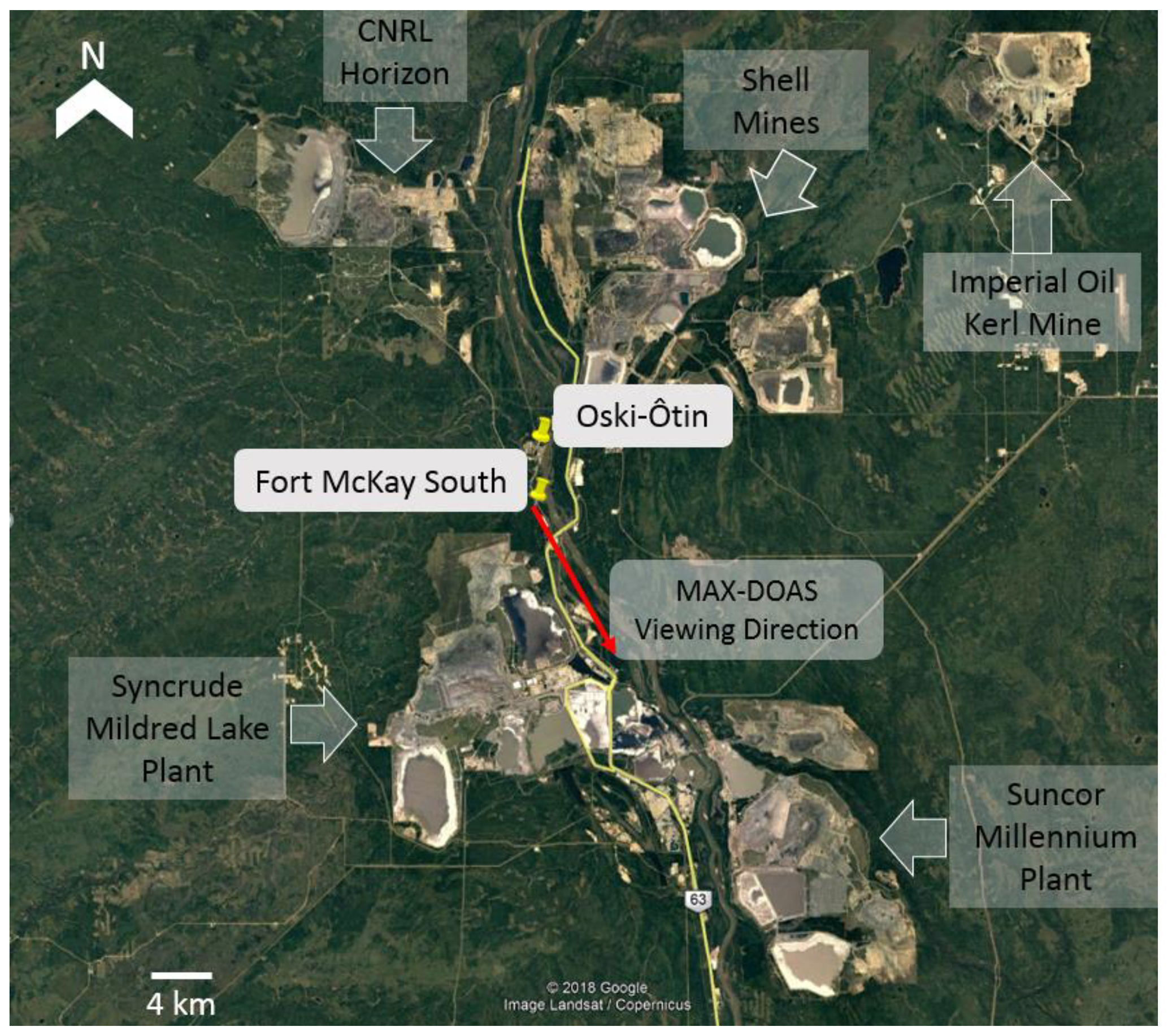
Figure 1Location of field sites Fort McKay South and Oski-Ôtin and major industry sources.
2.2 Instrumentation
The mini-MAX-DOAS instrument from Hoffmann Messtechnik GmbH measured scattered sunlight with a viewing azimuth angle of 155∘ south–south-east (SSE) at sequential viewing elevation angles 2, 4, 8, 15, 30 and 90∘ (zenith) above the horizon. The instrument consisted of a sealed metal box containing entrance optics, a UV fibre-coupled spectrograph, and all electronics. The instrument field of view was approximately 0.6∘. Incident light was focused on a cylindrical quartz lens (focal length =40 mm) into a quartz fibre that transmitted the light into the OceanOptics USB2000 spectrograph. The spectrograph detector was a Sony ILX511 linear silicon charge-coupled device (CCD) array (2048 pixels, pixel size 14 µm×200 µm, signal-to-noise ratio at full signal 250:1). The spectrograph had a spectral range of 290–433 nm, a 50 µm wide entrance slit, and a spectral resolution of ∼0.6 nm full width at half maximum (FWHM). The spectrograph was cooled by a Peltier stage to maintain the selected temperature (5∘C). Spectrometer data were transferred to a laptop computer via USB cable. The instrument was controlled using the software package DOASIS, which allowed automated measurements by JScript programs. The instrument was mounted on an elevated scaffold approximately 10 m above ground level (a.g.l.), at approximately the height of the surrounding forest canopy. Each recorded measurement spectrum was an average of 2000 measured spectra with an exposure time that varied between 50 and 200 ms, depending on the ambient light levels.
MAX-DOAS aerosol and trace gas retrieved data were inter-compared with data from various other instruments deployed during the campaign. Table 1 provides information on these instruments and papers that describe their operation.
Table 1Description and locations of the study instruments.

n/a: not applicable.
An active DOAS instrument located at the same site was used to retrieve mixing ratios of NO2 and SO2 at 3.5 m a.g.l. The active DOAS light path was pointed in a south–south-east direction, approximately parallel to the MAX-DOAS viewing azimuth angle (Fig. 1). Measurements of trace gases with the active DOAS system have been described previously (McLaren et al., 2010, 2012; Wojtal et al., 2011), although details have been changed in the current study. DOAS measurements were made using a modified DOAS 2000 Instrument (TEI Inc.) utilizing a 150 W high-pressure Xe arc lamp and a coaxial Cassegrain telescope. The outgoing beam traversed the atmosphere for 1.15 km (pathlength =2.3 km) at an average height of 3.5 m a.g.l., where it impacted a retroreflector array composed of 30 (5.08 cm diameter) hollow corner cubes mounted on a raiseable tower. The beam traversed through an exploration line cut (5–10 m wide by 2 km long) in a mature coniferous forest. Return light was collected with a 2 m×600 µm UV-transparent fibre-optic cable and spectrometer (Ocean Optics USB2000, Grating no. 10, λ=288–492 nm, 1800 lines mm−1, 2048 element CCD, 25 µm slit, UV2 upgrade, L2 lens). Integration times of 30–40 ms and 4000 averages gave ≈2 min resolution with detection limits (3σ) of 120 and 170 ppt for NO2 and SO2, respectively. Xenon lamp, Hg calibration, offset, and dark noise spectra were collected for spectral fitting with DOASIS software. A small diffuser was installed in the entrance of the fibre to lower atmospheric turbulence noise (Stutz and Platt, 1993) in addition to using an optical fibre bending mode mixer.
A Pandora spectral sun photometer at Oski-Ôtin measured in direct sun and zenith sun viewing modes to retrieve total atmospheric column VCDs of SO2 and NO2 with precisions (1σ) of 4.6×10¹⁵ and 0.3×10¹⁵ molecules cm−2, respectively (Fioletov et al., 2016). Tropospheric VCDs of NO2 were determined from the Pandora total column VCDs by subtracting stratospheric VCDs modelled using the PRATMO stratospheric photochemical box model (McLinden, 2000). PRATMO was used as described in Adams et al. (2016), except monthly mean OSIRIS ozone profiles (Degenstein et al., 2009) and MODIS surface reflectivities (McLinden et al., 2014) were employed. The Pandora SO2 VCDs presented are assumed to be representative of tropospheric SO2 VCDs since stratospheric SO2 was assumed to be negligible. Pandora trace gas and MAX-DOAS data were both available for inter-comparison for 4 d during the study. SO2 and NO2 mixing ratios were also measured from the air on board a Convair 580 research aircraft (Baray et al., 2018) using Thermo Scientific 43iTLE and 42i-TL analyzers, respectively, between 12 August and 7 September 2013, including a spiral ascent near Fort McKay South (3 September).
AODs at 380 and 340 nm were obtained from Level 2.0 AERONET data, measured by a second sun photometer at Oski-Ôtin. Aerosol extinction profiles at 532 nm from 0.1 to 12 km a.g.l. were retrieved using a ground-based, zenith-pointing lidar operated at Fort McKay South (Strawbridge, 2013). In this study, the lidar profiles from 0.1 to 4 km were considered in order to match the vertical observation extent of the MAX-DOAS. The lidar has the advantage over sun photometer instruments because it can determine the vertical profile of optical extinction rather than just a column-averaged value but has higher uncertainty when the S ratio is variable (Strawbridge, 2013). Aerosol extinction profiles are retrieved from the measurements of the laser return signal using a chosen S ratio value. The S ratio is the ratio of the volume extinction coefficient to the backscatter coefficient and dictates the signal strength of the received return of the lidar's pulsed laser source (Strawbridge, 2013). Lidar S ratios are known to be variable but are often estimated given the type of particles expected in an environment (Irie et al., 2015). The S ratio depends on the shape, size distribution, and chemical composition of the aerosol particles, as well as the relative humidity (Weitkamp, 2005). A constant lidar ratio (“S ratio”) of 25 was used for the lidar retrievals unless otherwise specified. S ratios were modelled using Mie scattering theory and measurements of surface-level particle composition and size distribution at Fort McKay South for various times during 23 August to determine temporal variability in the S ratio. Source code for the Mie scattering calculations can be found in Aggarwal et al. (2018).
Ground-level particle composition was measured using an Aerodyne high-resolution soot particle aerosol mass spectrometer (SP-AMS) (Lee et al., 2019). Particle size distributions were measured using Scanning Mobility Particle Sizer (SMPS) (“dry” line mode) and Aerodynamic Particle Sizer (APS) instruments (see supplementary information in Tokarek et al., 2018, for more details). Particle diameters measured by the SMPS and by the APS were 0.014–0.74 and 0.5–19.81 µm, respectively. Data from these instruments were combined to determine particle size distributions from 0.014 to 19.81 µm, assuming the particles were unit density. Use of “dry” line mode SMPS increased uncertainties in the size distributions because ambient aerosols have more volume than dry aerosols. However, even in the highest relative humidity range, the ambient aerosol had only 30 % more volume compared to the dry aerosol which, assuming spherical particles, only results in a maximum increase in particle diameter of 9 %. The resulting error is expected to be much smaller than other errors such as converting mobility and aerodynamic diameters to optical diameters.
A radio acoustic meteorological profiler (windRASS, model MFAS, Scintec, Germany) at Oski-Ôtin measured temperature, wind speed, and wind direction at 10 m intervals from 40 m to up to a maximum altitude of 800 m (Gordon et al., 2018).
2.3 MAX-DOAS data analysis
2.3.1 MAX-DOAS fitting
Trace gas differential slant column densities (dSCDs) were obtained using the DOAS technique (Platt et al., 2008) with DOASIS software (Institute of Environmental Physics, Heidelberg, Germany). All spectra were corrected for dark current and electronic offset and wavelength that were calibrated using a measurement of a Hg lamp. Table 2 shows the wavelength windows and fit components used to retrieve dSCDs of NO2, SO2, and O4. Cross sections were obtained from the MPI-Mainz UV/VIS Spectral Atlas of Gaseous Molecules of Atmospheric Interest (Keller-Rudek et al., 2013). Examples of spectral retrievals of the gases are shown in Fig. S2. Each non-zenith measured spectrum was fit against the closest zenith spectrum in time, also known as the Fraunhofer reference spectrum (FRS). The statistical error of the O4 dSCDs was molecules cm−2. The O4 error for off-axis measurements relative to the FRS are <6 % for angles below 30∘ and <10 % for the 30∘ measurements. The statistical fit errors of the SO2 and NO2 dSCDs were 0.4–1.2×10¹⁶ and 0.4–1.6×10¹⁵ molecules cm−2, respectively. Uncertainties in the absorption cross sections result in systematic errors in the retrieved dSCDs. The reported uncertainty in the SO2 and NO2 absorption cross sections used is approximately 3 % (Bogumil et al., 2003). The absolute value of the O4 cross section and its dependence on temperature is uncertain. Some studies suggest that the absolute value of the cross section may be overestimated by up to 25 %, requiring the use of a scaling factor (Clémer et al., 2010; Wagner et al., 2002, 2009, 2019). However, Frieß et al. (2011) found that the best results for measured O4 dSCDs and the vertical profiles of aerosol extinction retrieved from them were achieved without a scaling factor. Irie et al. (2015) found that a scaling factor of 1.25 resulted in an overestimation of near-surface aerosol extinction coefficients (AECs) but also reduced residuals at high viewing elevation angles. Wagner et al. (2019) found that measured and radiative transfer modelled O4 absorptions showed good agreement on one study day but poor agreement on the second. A scaling factor was not used for the O4 fitting in this study because of the lack of consensus on the need for a scaling factor within the DOAS community and the good agreement between the MAX-DOAS and smoothed lidar AODs for the 23 August data (see Sect. 3.1.2).
The SO2 fitting range was determined based on an experiment using an SO2 calibration cell from Resonance Ltd. with a slant column density (SCD) of 2.2×10¹⁷ (±10 %) molecules cm−2 placed inside the MAX-DOAS telescope. Scattered solar light spectra were recorded around solar noon at multiple viewing elevation angles above the horizon, followed by a 90∘ measurement without the cell (the FRS). For each of the measured spectra, dSCDs of SO2 were fit in DOASIS by varying the fitting windows in ∼0.3 nm increments with a range of lower and upper limits of 303–318 and 309–340 nm, respectively. The fit components are the same as in Table 2. See Sect. S2 in the Supplement for details. The NO2 and O4 fitting ranges were from McLaren et al. (2010) and Frieß et al. (2011), respectively.
2.3.2 Retrieval of vertical profiles from MAX-DOAS dSCDs using optimal estimation
Aerosol and trace gas profiles were retrieved using a two-step approach: (1) aerosol extinction profiles were retrieved from measured MAX-DOAS O4 dSCDs, and (2) aerosol extinction profiles were used as forward model parameters for retrieval of NO2 and SO2 profiles from dSCDs of NO2 and SO2, respectively. Vertical profiles were determined from dSCDs using retrieval algorithms based on the Rodgers (2000) optimal estimation technique (Frieß et al., 2011, 2016, 2019). Generally, the desired state of the atmosphere (x) can be estimated from remote sensing measurements (y) using a forward model F:
where ε is the measurement error and b is the vector of model parameters that are assumed to be known and not determined by the modelling, such as aerosol microphysical properties. In this study, the SCIATRAN radiative transfer model was used as the forward model (Rozanov et al., 2005).
The optimal estimation method determined the most probable atmospheric state, , based on a set of measurements, y, and an a priori state vector, xa. The xa was the best guess of the vertical profile to be retrieved. The was the aerosol extinctions or the trace gas mixing ratios at a series of altitude intervals for the aerosol retrieval and trace gas retrievals, respectively. The y was the O4 dSCDs and the trace gas dSCDs measured at different angles, for the aerosol and trace gas retrievals, respectively. The agreements between measured and modelled dSCDs based on linear regressions for the retrievals are shown in Sect. S8.1 in Tables S10 and S11, as well as typical degrees of free of signal for the aerosol and trace gas retrievals. Note that in our retrievals, y was the dSCDs measured at sequential elevation angles during 20 min periods before 17:00 local time (LT) and during 30 min periods after 17:00 LT. The wavelengths for the optimal estimation retrievals of O4, NO2, and SO2 were 360.8, 422.5, and 318.0 nm, respectively.
The optimal estimation solution is the maximum a posteriori (MAP) solution, which selects the most probable state from the set of possible states described by maximizing the probability of x occurring given the observations y (Rodgers, 2000). The MAP solution is found by minimizing the cost function (χ2):
where Sa and SE are the error covariance matrices associated with the a priori and measurement vectors, respectively (Rodgers, 2000). The retrieval yields important quantities that allow the characterization of the retrieval. These include the weighting function, , which quantifies the sensitivity of the measurement towards the atmospheric state, and the averaging kernel matrix, , which quantifies the vertical resolution of the retrieval. A describes the sensitivity of the retrieved profile to changes in the true atmospheric profile. Rows of A are averaging kernels for each altitude interval in the retrieved profile. The full width half maximum (FWHM) of each kernel gives an estimate of the retrieval's vertical resolution at height z. Each averaging kernel ideally peaks at a magnitude of 1.0 at the height of the kernel. However, the peak value of a kernel is generally less than 1.0 due to finite vertical resolution and may peak at a slightly different height, resulting in the smoothing of the true atmospheric profile into the retrieved profile.
Aerosol extinction retrievals
Retrieval of aerosol extinction profiles was non-linear since the aerosol extinction affects the radiative transfer in the forward model. The input for the aerosol retrieval was the measurement vector of the O4 dSCDs at different elevation angles and an a priori state vector that decreased exponentially with altitude with a scale height of 0.6 km and a surface magnitude of 0.1 km−1. A single a priori profile choice is preferable for a set of consecutive measurements where information content is potentially limited since the a priori will always have some impact on the retrieved profile (Rodgers, 2000). Otherwise, diurnal and day-to-day trends in the retrieved profiles due to real atmospheric changes could be indistinguishable from changes due to a variable a priori profile. Sensitivity studies of the a priori choice were conducted by varying one a priori parameter while keeping the remainder of settings the same: Gaussian shape, Boltzmann shape, scale height of 0.3 km, or scale height of 1.2 km. The results of the sensitivity studies are shown in Sect. S8.2.
Our aerosol retrieval used an iterative algorithm based on the Levenberg–Marquart method (Levenberg, 1944; Marquardt, 1963). For aerosol retrievals, the weighting function K is calculated using the a priori xa and the measurement vector y. The K of each retrieval depended on the state vector and changed depending on the determined aerosol extinction profile. The height resolution of the aerosol extinction vertical profile grid was 100 m with a maximum height of 4 km. A detailed description of the aerosol retrieval algorithm can be found in Frieß et al. (2006).
Trace gas retrievals
The retrievals of NO2 and SO2 vertical profiles were linear because these weak absorbers do not significantly impact the radiative transfer. The inputs for the NO2 and SO2 retrievals were the measurement vectors of the NO2 and SO2 dSCDs at different elevation angles, respectively, and an a priori state vector that decreased exponentially (scale height is 0.6 km and surface magnitude is 30 and 10 ppb for SO2 and NO2, respectively). Sensitivity studies of the a priori choice were conducted by varying one a priori parameter while keeping the remainder of settings the same: Gaussian shape, Boltzmann shape, scale height of 0.3 km, or scale height of 1.2 km. The results of the sensitivity studies are shown in Sect. S8.2.
In this linear case, the forward model is independent of the atmospheric state x, and the weighting function matrix represents the forward model.
In our retrieval, the box air mass factors (AMFs) that are components of K were modelled using the radiative transfer model in SCIATRAN (Deutschmann et al., 2011; Frieß et al., 2010; Rozanov et al., 2005). The aerosol profiles retrieved in step 1 were used to recalculate the box AMFs for each trace gas retrieval since the extinction profiles varied. The height resolution of the trace gas vertical profile grid was 100 m with a maximum height of 4 km a.g.l.
Determination of retrieval errors
The retrieval covariance matrix quantifies the error of the state vector and is the sum of the independent sources of error: smoothing error Ss, representing the retrieval's limited vertical resolution, and the retrieval noise SM, representing the uncertainty due to errors in the measurement (). The error covariance matrix produced by the retrieval does not include model parameter errors or forward model errors (Frieß et al., 2006). The error covariance matrix is calculated following Eq. (4):
SE and Sa are the measurement and a priori covariance matrices, respectively. In our retrievals, Sa was determined by setting the relative error of the a priori to 100 % and the extra-diagonal terms were set to zero. The SE was the diagonal matrix of errors of the retrieved dSCDs as determined by the DOASIS retrievals.
2.3.3 Conversion of other instruments' data for comparison to MAX-DOAS data
Lidar and AERONET extinction data were converted to the MAX-DOAS aerosol retrieval wavelength of 361 nm following Eq. (5):
Equation (5) accounts for the dependence of aerosol extinction on wavelength based on the Angstrom exponent, ∝. AERONET 300–500 and 340–440 nm Angstrom exponents were used to convert the 532 nm lidar aerosol extinctions and the 380 and 340 nm AERONET AODs, respectively. The two resulting AERONET AODs at 361 nm were then averaged. The Angstrom exponent was assumed to be constant with altitude and representative of both field sites. The similarity in trends in AODs and trace gas VCDs between the two sites can indicate when the Angstrom exponent determined from Oski-Ôtin was valid for both sites.
Due to the limited vertical resolution of the MAX-DOAS measurements, MAX-DOAS vertical profiles of aerosol extinction and AODs can only be directly compared to lidar profiles and AODs after smoothing the 361 nm lidar profiles using the MAX-DOAS averaging kernel matrix, A (Rodgers and Connor, 2003). The lidar AODs referred to in the paper below and shown in plots are the smoothed AODs determined by vertically integrating the smoothed lidar vertical profiles of extinction at 361 nm unless otherwise stated.
The lidar profiles were averaged into the same altitude and temporal intervals as the MAX-DOAS retrievals and then smoothed using the respective matrix A following Eq. (6):
where xs is the smoothed lidar profile, xa is the MAX-DOAS retrieval a priori profile, and xL is averaged lidar profile. xs represents the (noise-free) vertical profile that the MAX-DOAS retrieval would produce if xL was the true atmospheric profile given the variable sensitivity of the MAX-DOAS retrieval with altitude. The deviation of xs from xL at each altitude depends on xa and the sensitivity of the MAX-DOAS to the atmosphere at that altitude. MAX-DOAS sensitivity to the true atmospheric state decreases with increasing altitude (Frieß et al., 2006) with typical height resolutions of ∼200 m at lower altitudes, increasing to ∼700 m at higher altitudes. Therefore, the smoothing is generally expected to smooth the true profiles towards lower altitudes. Also, even if the two instruments viewed the same air mass, the retrieved and smoothed profiles are expected to differ at least slightly due to two factors. The first factor is the retrieval noise Gε, which is unknown since the true measurement error ε is unknown. G is the gain matrix, which describes the retrieval's sensitivity to the measurements. The true smoothed profiles would be described using the following Eq. (7):
The second factor is that lidar vertical profiles are observed straight up, are measured only above 100 m a.g.l., and are the least sensitive close to the surface. The 0–100 m a.g.l. extinction in the lidar profiles was assumed to be equal to the average extinction measured between 100 and 200 m a.g.l. but the vertical profiles may have been variable below 150 m a.g.l. Uncertainty in the lidar vertical profiles is greatest in the lowest 150 m a.g.l., introducing uncertainty into the smoothed lidar profiles.
Error bars on the MAX-DOAS AODs, VCDs, and mixing ratios shown in figures were obtained from the optimal estimation retrieval. Error bars on the lidar and AERONET AODs are the standard error of the temporally averaged values since these instruments have a finer time resolution than the MAX-DOAS retrievals. Error bars on the active DOAS mixing ratios are the root-sum-square errors of the standard error of the averaged values and the average error reported by the respective DOASIS retrievals. Error bars on the Pandora VCDs are root-sum-square errors of the standard error of the average values and the reported instrumental precision. Deming fit linear regressions were performed using the Monte Carlo method, which included the errors on the x and y data, with the “linfitxy” function in MATLAB (Browaeys, 2017). The 23 August and 3 September AERONET and Pandora data were also correlated with MAX-DOAS and lidar data by subtracting 30 min from the Oski-Ôtin data to account for the time of air mass transport between the Fort McKay South and Oski-Ôtin given the wind speeds.
This paper discusses results from largely cloud-free days when industrial plumes were observed (23 August and 3, 4, 6, and 7 September) and 1 d with clean conditions (5 September). The 9 d are not discussed due to the presence of clouds most of the day.
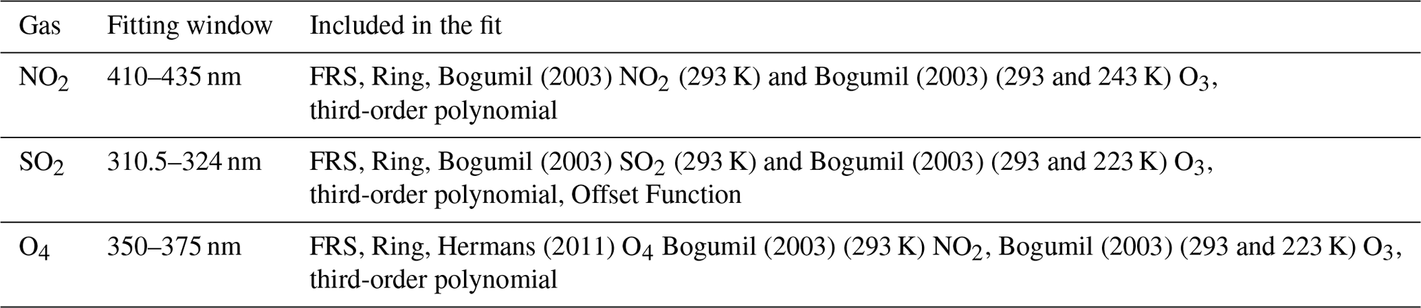
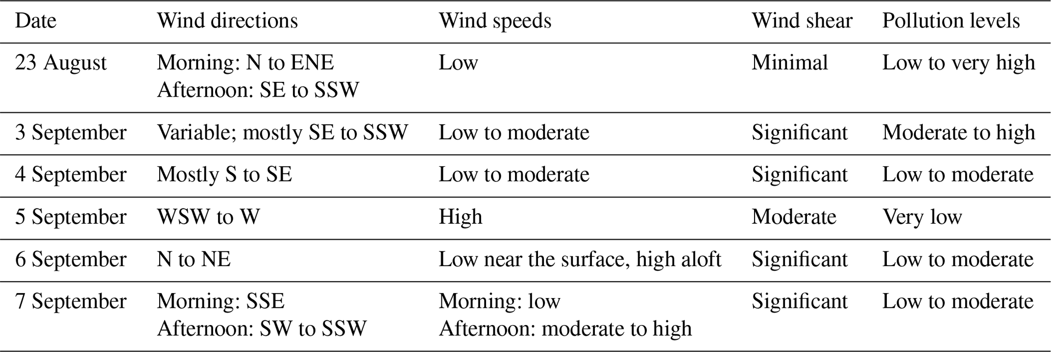
Vertical profiles of wind speed and wind direction measured by the windRASS are shown in Figs. 2 and 3, respectively. A summary of wind conditions and pollution levels for each day is shown in Table 3.
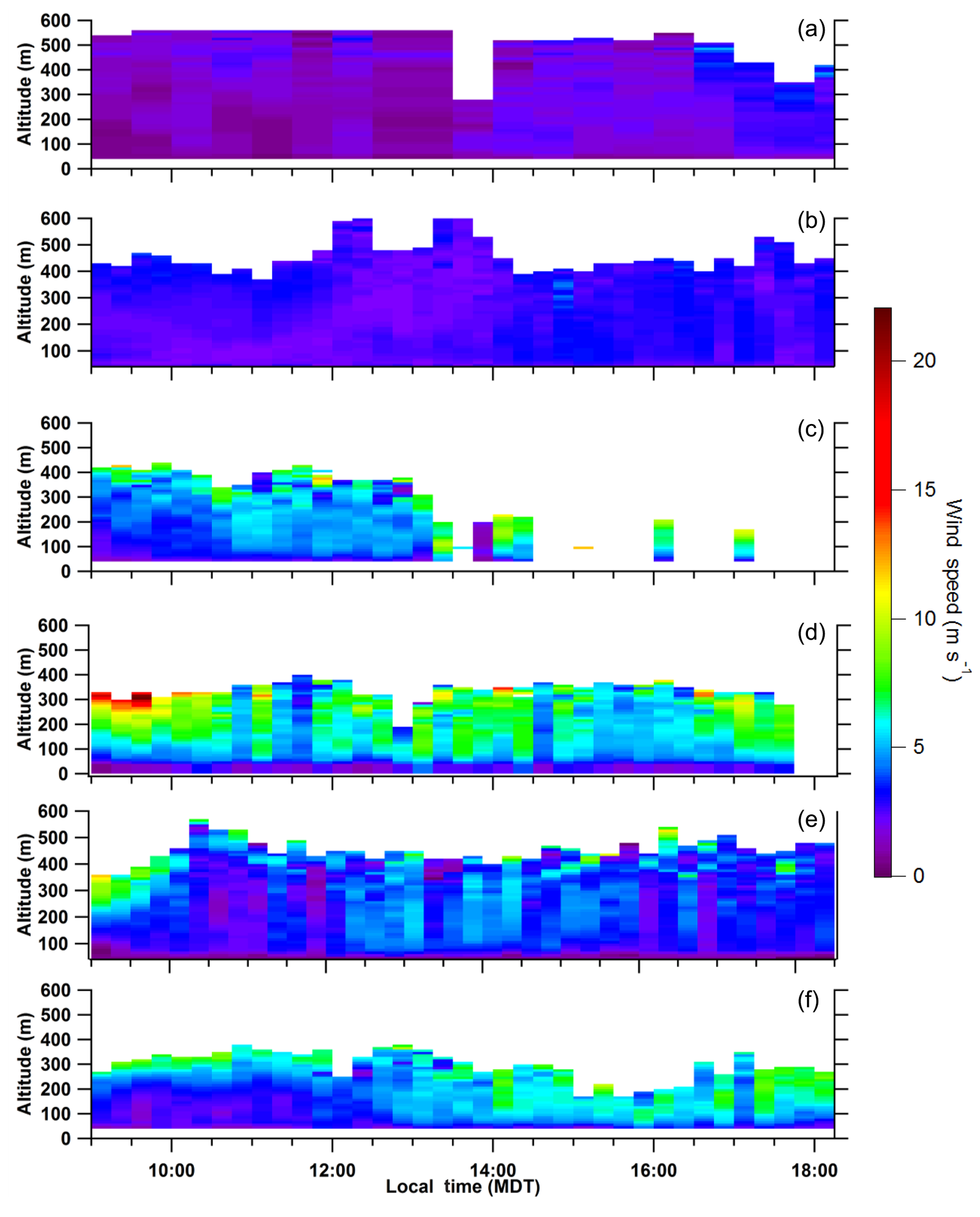
Figure 2Vertical profiles of wind speed: 23 August (a), 3 September (b), 4 September (c), 5 September (d), 6 September (e), and 7 September (f).
Figure 3Vertical profiles of wind direction: 23 August (a), 3 September (b), 4 September (c), 5 September (d), 6 September (e), and 7 September (f).
Table 3Daytime wind and pollution conditions during the study days.
The 23 August plume exhibited the greatest enhancements in aerosol and trace gas pollution during the study. Wind directions in the morning were northerly to east–north-easterly and south-easterly to south–south-westerly in the afternoon. Winds were of relatively low speed with minimal wind shear. The pollution enhancement periods were associated with southerly (S) winds, suggesting that air masses rich in industrial emissions originated from the Syncrude and Suncor mining areas south of the sites (Fig. 1). The pollution enhancements impacted both sites (AMS 13 and Oski-Ôtin).
The 3 September plume exhibited moderate pollution levels. Pollution data are only presented from 11:00 LT onwards due to the presence of clouds before this time. Wind directions varied from south-easterly to south–south-westerly with occasional south-westerly to north-westerly winds. Significant wind shear was observed in the vertical profiles of wind. The pollution enhancements impacted both sites.
The 4 September plume exhibited moderate pollution levels. Wind directions were frequently southerly to south-easterly with intermittent periods of south-westerly and north-westerly winds. Significant wind shear was observed: wind directions tended to rotate clockwise from south–south-easterly near the surface to north-easterly as altitude increased. The limited afternoon wind data suggest north-westerly winds. Wind speeds were low to moderate, tending to increase with altitude. The pollution enhancements impacted both sites.
The 5 September plume exhibited the cleanest conditions and greatest wind speeds during the study. Winds were west–south-westerly to westerly. Both sites were impacted by air masses that passed over boreal forests.
The 6 September plume exhibited low to moderate pollution enhancements in the morning with low-pollution conditions in the afternoon. Winds were northerly to north-easterly but varied over time and with altitude. Wind speeds tended to be low at the surface but moderate to large at higher altitudes; significant wind shear was present. Fort McKay South was impacted by emissions from facilities north of the sites: Shell Jackpine and Muskeg River Mines, CNRL Horizon, and Imperial Oil.
The 7 September plume exhibited moderate to low pollution. Wind directions were south–south-east during the morning and south-west to south–south-west during the afternoon. Significant wind shear was observed in the lowest 400 m a.g.l. between 09:00 and 11:00 LT and during the afternoon around 16:00 LT. Different air masses may have impacted the two sites.
3.1 Inter-comparisons of MAX-DOAS aerosol retrievals with lidar and AERONET data
The AODs from the MAX-DOAS, lidar, and AERONET sun photometer instruments exhibited similar temporal trends on 23 August and 3, 4, 5, and 7 September (Figs. 4–9a). Note that the measured and optimal estimation modelled O4 dSCDs showed good agreement for all these days with linear regression slopes of 0.99 and R2=0.91–0.98 (Table S10). The MAX-DOAS AODs were statistically different from the lidar and AERONET AODs for approximately half the data, even when the two sites experienced the same air masses. This result is expected based on three factors: (1) the different vertical extents of the atmosphere observed by the instruments, (2) temporal variability in the lidar S ratio, and (3) the limited sensitivity of the MAX-DOAS measurements at higher altitudes. These factors will be discussed below to evaluate the performance of the MAX-DOAS AOD retrievals under various atmospheric conditions.

Figure 4The 23 August AODs from MAX-DOAS, lidar (S ratio 14:30 LT), and AERONET (30 min) (a); AODs from MAX-DOAS, lidar (S ratio =25 sr), and AERONET (b); MAX-DOAS and Pandora SO2 VCDs (c); MAX-DOAS and Pandora NO2 VCDs (d); MAX-DOAS 0–100 m and active DOAS SO2 mixing ratios (e); MAX-DOAS 0–100 m and active DOAS NO2 mixing ratios (f); MAX-DOAS VCDs and active DOAS mixing ratios of SO2 (g); and MAX-DOAS VCDs and active DOAS mixing ratios of NO2 (h). MAX-DOAS error bars were obtained from the optimal estimation retrieval. Error bars on the lidar and AERONET AODs are the standard error of the temporally averaged values. Error bars on the Pandora VCDs and active DOAS mixing ratios are root-sum-square errors of the standard error from temporal averaging and instrumental precision and the DOASIS retrieval error, respectively. See Sect. 2.3.3 for details.
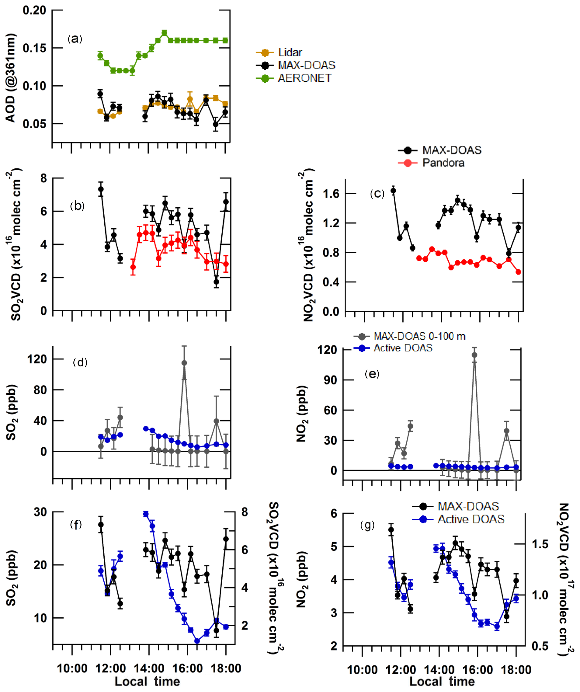
Figure 5The 3 September AODs from MAX-DOAS, lidar, and AERONET (a); MAX-DOAS and Pandora SO2 VCDs (b); MAX-DOAS and Pandora NO2 VCDs (c); MAX-DOAS 0–100 m and active DOAS SO2 mixing ratios (d); MAX-DOAS 0–100 m and active DOAS NO2 mixing ratios (e); MAX-DOAS VCDs and active DOAS mixing ratios of SO2 (f); and MAX-DOAS VCDs and active DOAS mixing ratios of NO2 (g). MAX-DOAS error bars were obtained from the optimal estimation retrieval. Error bars on the lidar and AERONET AODs are the standard error of the temporally averaged values. Error bars on the Pandora VCDs and active DOAS mixing ratios are root-sum-square errors of the standard error from averaging and instrumental precision and the DOASIS retrieval error, respectively. See Sect. 2.3.3 for details.
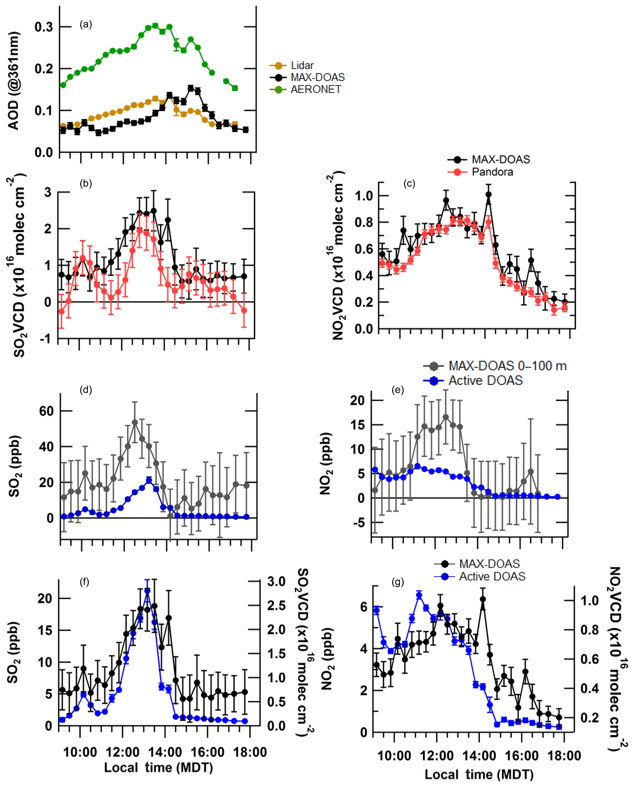
Figure 6The 4 September AODs from MAX-DOAS, lidar, and AERONET (a); MAX-DOAS and Pandora SO2 VCDs (b); MAX-DOAS and Pandora NO2 VCDs (c); MAX-DOAS 0–100 m and active DOAS SO2 mixing ratios (d); MAX-DOAS 0–100 m and active DOAS NO2 mixing ratios (e); MAX-DOAS VCDs and active DOAS mixing ratios of SO2 (f); and MAX-DOAS VCDs and active DOAS mixing ratios of NO2 (g). MAX-DOAS error bars were obtained from the optimal estimation retrieval. Error bars on the lidar and AERONET AODs are the standard error of the temporally averaged values. Error bars on the Pandora VCDs and active DOAS mixing ratios are root-sum-square errors of the standard error from averaging and instrumental precision and the DOASIS retrieval error, respectively. See Sect. 2.3.3 for details.
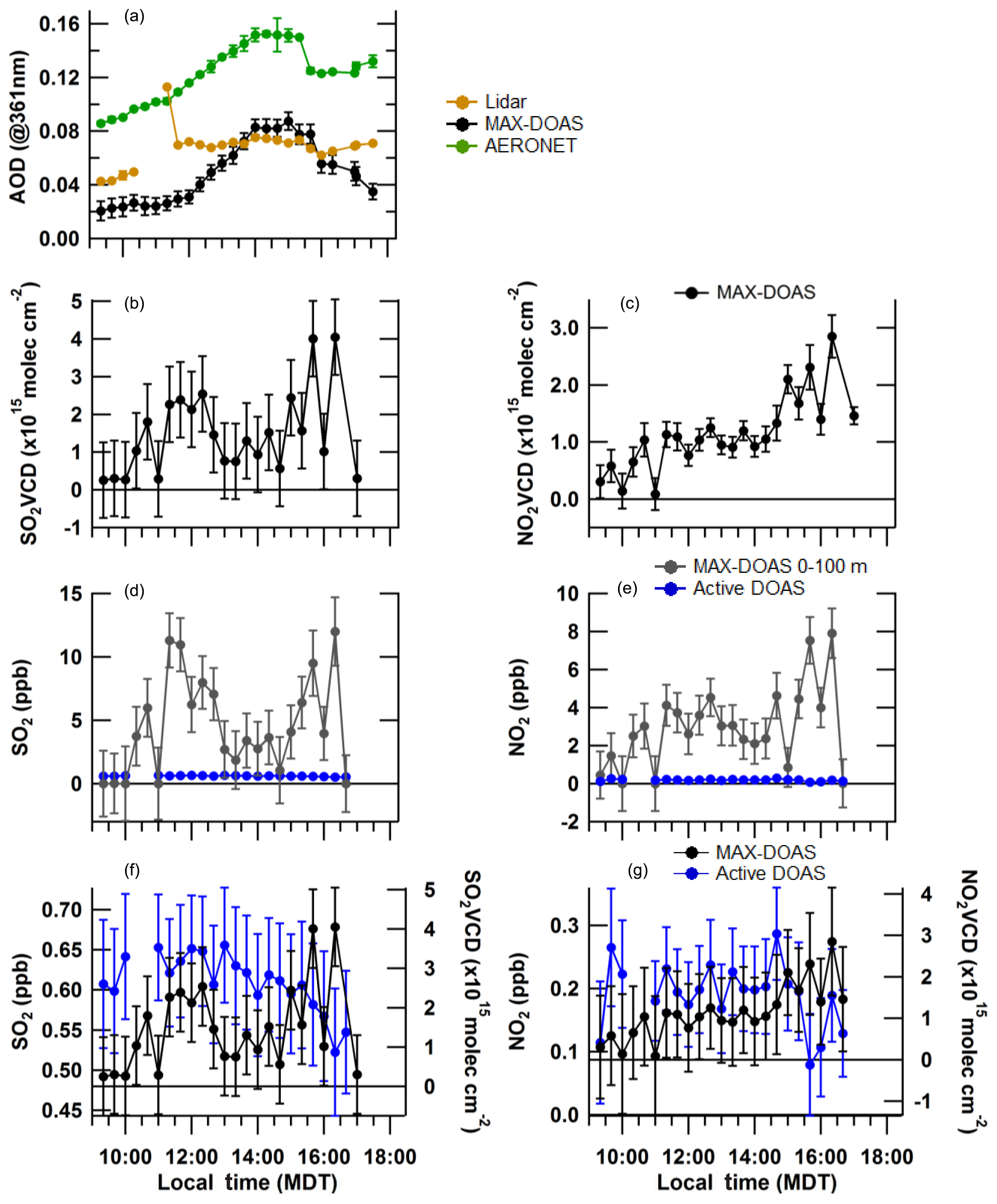
Figure 7The 5 September AODs from MAX-DOAS, lidar, and AERONET (a); MAX-DOAS SO2 VCDs (b); MAX-DOAS NO2 VCDs (c); MAX-DOAS 0–100 m and active DOAS SO2 mixing ratios (d); MAX-DOAS 0–100 m and active DOAS NO2 mixing ratios (e); MAX-DOAS VCDs and active DOAS mixing ratios of SO2 (f); and MAX-DOAS VCDs and active DOAS mixing ratios of NO2 (g). MAX-DOAS error bars were obtained from the optimal estimation retrieval. Error bars on the lidar and AERONET AODs are the standard error of the temporally averaged values. Error bars on the active DOAS mixing ratios are root-sum-square errors of the standard error from averaging and the DOASIS retrieval error. See Sect. 2.3.3 for details.
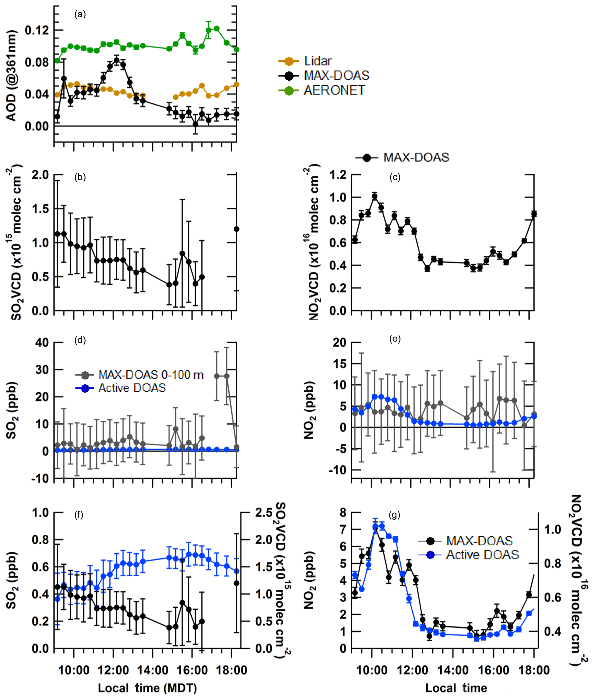
Figure 8The 6 September AODs from MAX-DOAS, lidar, and AERONET (a); MAX-DOAS SO2 VCDs (b); MAX-DOAS NO2 VCDs (c); MAX-DOAS 0–100 m and active DOAS SO2 mixing ratios (d); MAX-DOAS 0–100 m and active DOAS NO2 mixing ratios (e); MAX-DOAS VCDs and active DOAS mixing ratios of SO2 (f); and MAX-DOAS VCDs and active DOAS mixing ratios of NO2 (g). MAX-DOAS error bars were obtained from the optimal estimation retrieval. Error bars on the lidar and AERONET AODs are the standard error of the temporally averaged values. Error bars on the active DOAS mixing ratios are root-sum-square errors of the standard error from averaging and the DOASIS retrieval error. See Sect. 2.3.3 for details.
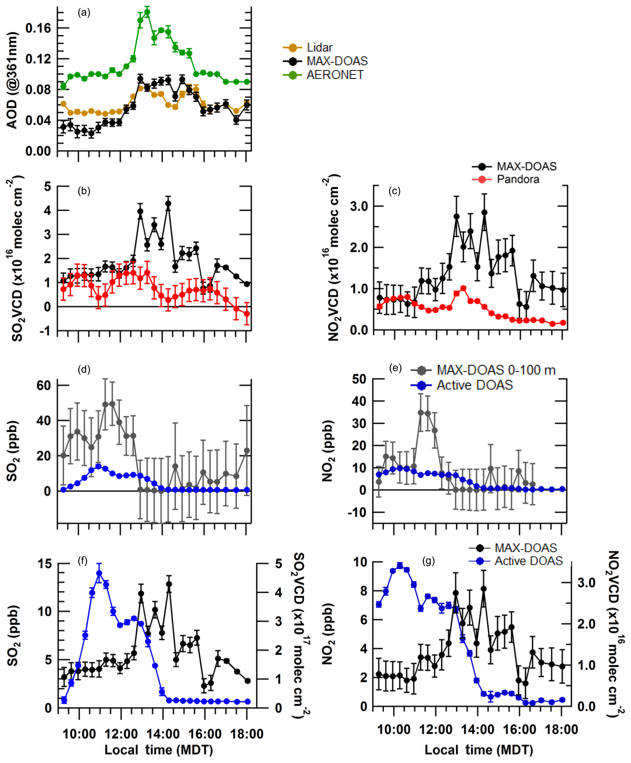
Figure 9The 7 September AODs from MAX-DOAS, lidar, and AERONET (a); MAX-DOAS and Pandora SO2 VCDs (b); MAX-DOAS and Pandora NO2 VCDs (c); MAX-DOAS 0–100 m and active DOAS SO2 mixing ratios (d); MAX-DOAS 0–100 m and active DOAS NO2 mixing ratios (e); MAX-DOAS VCDs and active DOAS mixing ratios of SO2 (f); and MAX-DOAS VCDs and active DOAS mixing ratios of NO2 (g). MAX-DOAS error bars were obtained from the optimal estimation retrieval. Error bars on the lidar and AERONET AODs are the standard error of the temporally averaged values. Error bars on the Pandora VCDs and active DOAS mixing ratios are root-sum-square errors of the standard error from averaging and instrumental precision and the DOASIS retrieval error, respectively. See Sect. 2.3.3 for details.
3.1.1 Impact of instrumental vertical sensitivity on AOD
AERONET AODs were generally significantly greater than MAX-DOAS and lidar AODs, except during the greatest pollution events (Figs. 4–9a). During the low-pollution day of 5 September, AERONET AODs reached a maximum of 0.15±0.00 while maximum MAX-DOAS AODs were 0.08±0.01 (Fig. 4b). On 5 September the MAX-DOAS and AERONET AODs had a slope of linear correlation of 1.04±0.08 (R2=0.77) but had a linear intercept of km−1. This negative intercept can be attributed to aerosol loading above the boundary layer that was observed by the sun photometer but not by the MAX-DOAS. This result is expected because the AERONET sun photometer observed aerosol extinction throughout the entire column (tropospheric and stratospheric) while the MAX-DOAS and smoothed lidar profiles observed up to 4 km. Further, the MAX-DOAS retrieved and smoothed lidar profiles likely only represented aerosol extinction below 2 km because of the exponentially decreasing a priori profiles used and the decreasing sensitivity of the MAX-DOAS retrieval with increasing altitude (see Sect. S8 for explanation of the a priori shape and scale height choice). The MAX-DOAS and smoothed lidar AODs are, therefore, expected to be significantly smaller than the AERONET AODs when the aerosol extinction in the boundary layer was “clean” and contributed a small fraction to the total tropospheric extinction (e.g., Fig. 10; 23 August, 09:10 LT). MAX-DOAS AODs were also significantly smaller than AERONET AODs even under moderately polluted conditions when the magnitudes of the aerosol extinction remained enhanced compared to background above the boundary layer. For example, on 4 September the extinctions between the boundary layer top and 4 km could be relatively large, about one-third of the near-surface extinctions (Figs. 10, 15a and S9a), leading to much smaller MAX-DOAS AODs than AERONET AODs (Fig. 6a). Note that increasing the scale height of the 4 September a priori profile from 0.6 to 1.2 km only slightly increased the MAX-DOAS AODs with a linear regression slope of 1.14±1.13 and intercept km−1 (Table S21 and Figs. S17, S24). The AODs from both a priori profiles were ∼50 % of the AERONET AOD values, an expected result since a significant contribution to the total AOD was expected to be present >3 km (Table S21, Fig. S9a). Aerosol loading can be non-trivial in the free troposphere since fine-mode particles can remain in the atmosphere for days (Zhong and Zaveri, 2017). Dust and smoke aerosol types are transported most efficiently to the free troposphere from the boundary layer compared to other types. Once in the free troposphere, aerosols have much longer residence compared to within the boundary layer. Therefore, enhanced loading of dust and smoke aerosols present in the free troposphere in the AOSR may be due to local sources since dust and smoke are emitted by the industrial activities and biomass burning but also could be transported long distances (e.g., originating from fires in British Columbia). Forest fire smoke has been observed above the boundary layer by airborne lidar measurements in AOSR (see Figs. 12 and 13 and discussion of elevated forest fire plumes in Aggarwal et al., 2018). Therefore, the aerosol extinction above the boundary layer in the AOSR could contribute to a significant fraction of the total atmospheric AOD on certain days depending on the emission and transport of aerosols. Globally, Bourgeois et al. (2018) found that the monthly averaged fractional contribution of the free troposphere extinction to the total AOD obtained from satellite observations was greater in northern mid-latitudes (25 %) compared to southern mid-latitudes (13 %), attributed to the larger number of emission sources and convection activity. While monthly average contribution was 25 %, the contribution likely varies significantly on a day-to-day basis, particularly in a region such as the AOSR that has numerous emission sources, both locally and upwind. The lidar measurements indicate that the contribution of the AOD above 2 km can vary significantly, as indicated by a comparison of aerosol extinction vertical profiles from 4 September and 23 August (Fig. S9). These results indicate that the ratio of the MAX-DOAS AODs to AERONET AODs depends on the location of the aerosol extinction within the tropospheric profile. The use of simple linear regressions to evaluate the performance of MAX-DOAS AOD retrievals using sun photometer AODs may be appropriate only when the aerosol extinction in the boundary layer dominates the total tropospheric AOD.
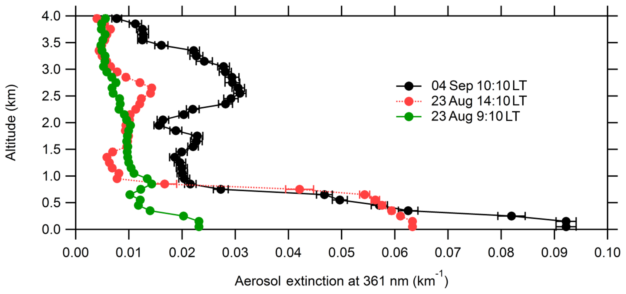
Figure 10Examples of lidar vertical profiles of aerosol extinction (averaged into MAX-DOAS retrieval height intervals and times) on 23 August and 4 September.
3.1.2 Impact of S ratio variability on lidar AODs
MAX-DOAS AODs significantly exceeded the smoothed lidar AODs during the most polluted periods (Fig. 4b). This result is unexpected, given that the instruments' AODs should ideally be equal when the instruments observed the same air masses. However, the deviation can be explained by variation in the lidar S ratio. The S ratio of 25 sr (steradian) appears accurate during relatively clean periods (e.g., 5 September, 23 August morning), but an underestimation under the industrially polluted conditions of the afternoon of 23 August (Figs. 4b and 12). Modelled S ratios for 23 August were 21–28 sr during the low-pollution morning and 36–44 sr during the peak pollution enhancement at ∼ 16:50 LT (Table 4). The morning S ratios were calculated using the refractive indices of toluene or kaolinite based on the dominance of organic particles and dust in the region during background atmospheric conditions (Fig. 11a). The afternoon S ratios were modelled using the refractive index of sulfate particles based on the significant enhancement in sulfate particle loading (Fig. 11a). Increased loading of sulfate particles tends to increase the S ratio. Note that the 16:50 LT S ratios were greater than the morning S ratios for all refractive indices because the particle size distribution of the industrial plume (fine-mode dominated) increased the S ratio. The modelled variability in the S ratio is supported by lidar measurements in the AOSR in 2018 that allowed determination of temporal and vertical variability in the S ratio (Strawbridge et al., 2018). Measured S ratios ranged from 20 to 60 sr within the boundary layer at Oski-Ôtin in 2018 (Fig. S6).
Table 4Modelled lidar S ratios (sr) for selected periods on 23 August using refractive indices (RIs) of different particles.
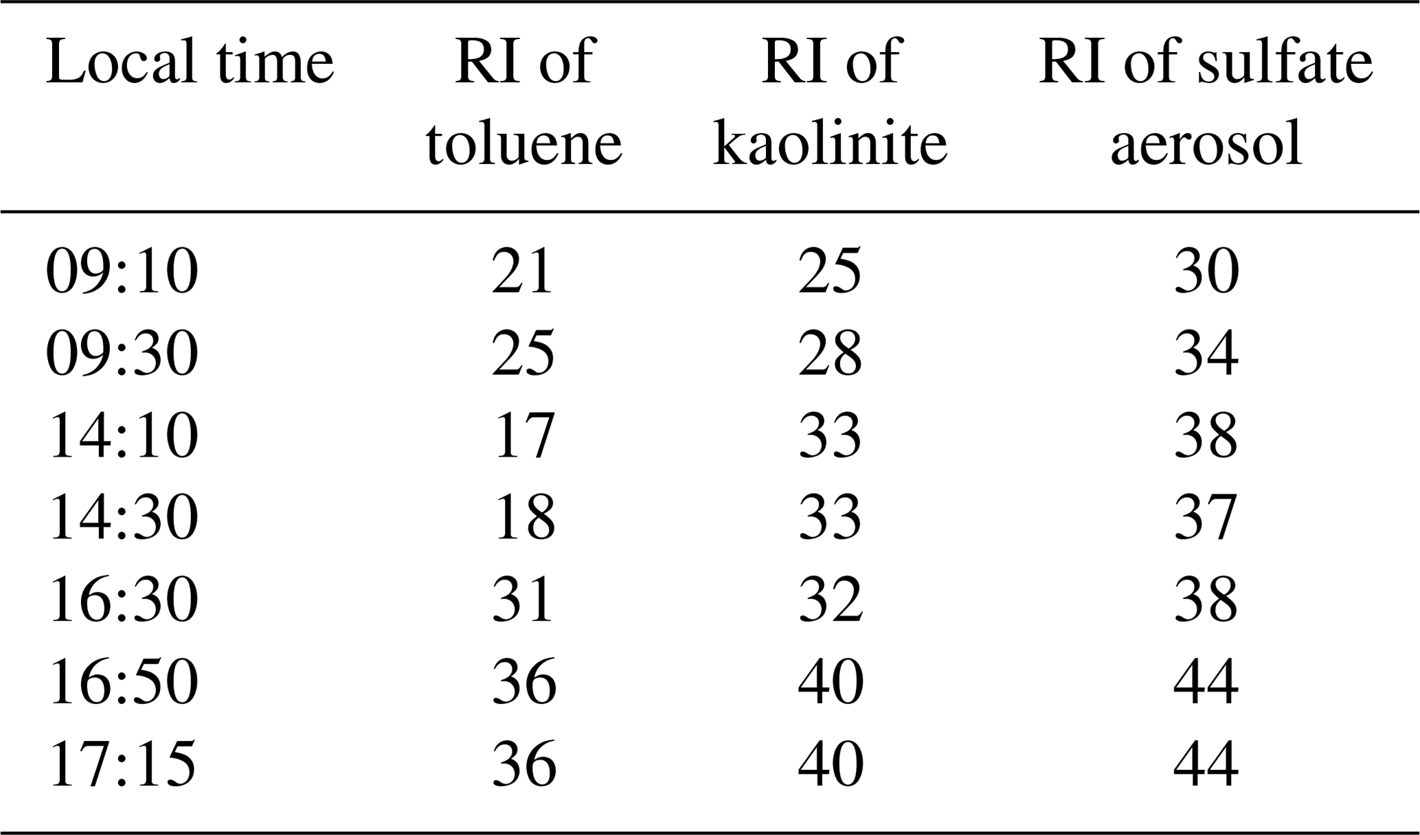
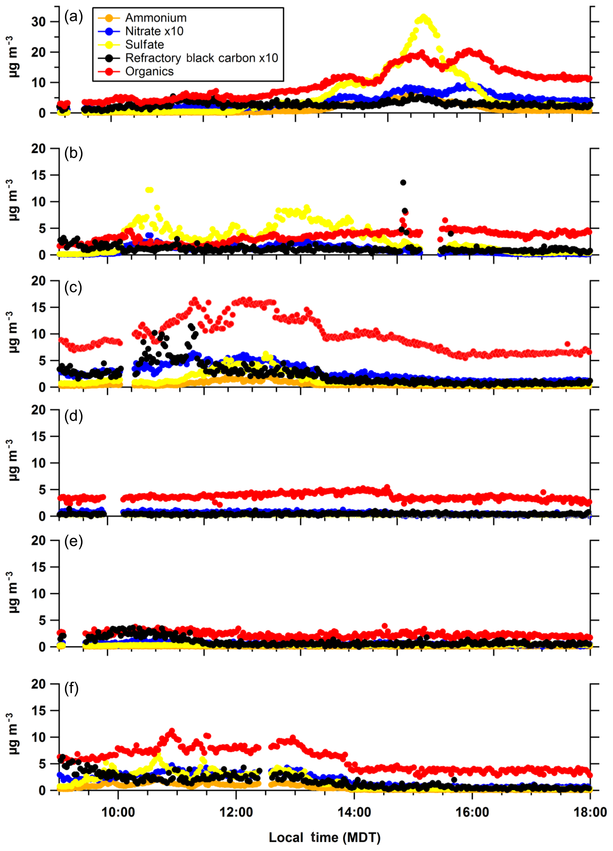
Figure 11Near-surface particle compositions on 23 August (a), 3 September (b), 4 September (c), 5 September (d), 6 September (e), and 7 September (f). Note the different y axis scale for 23 August and that nitrate and refractory black carbon are shown multiplied by 10.
Based on these results, lidar vertical profiles of aerosol extinction were retrieved using an S ratio of 44 sr for the extinction below the free troposphere after 14:30 LT on 23 August. As shown in Fig. 4a, the updated lidar AODs are in more reasonable agreement with the MAX-DOAS and AERONET AODs compared to the original lidar AODs shown in Fig. 4b. The linear regression of the MAX-DOAS and updated lidar AODs has a slope of 1.15±0.02 with an intercept of (R2=0.97) instead of the 2.18±0.03 found for the original lidar AODs (R2=0.97) (Table S3). Modelling S ratios using particle data measured at the near-surface appears to be valid during 23 August because the vertical profile was relatively well mixed. A well-mixed boundary layer was indicated by the similarity in temporal trends between the active DOAS mixing ratios and MAX-DOAS VCDs and between the AODs and the surface particle loading (Figs. 4g, h and 11a). However, if the distribution of particles in space is inhomogeneous, this method cannot be used to determine the S ratio of the total boundary layer.
Results from 3 and 6 September illustrate that near-surface measurements of particle properties can be invalid for modelling the total column S ratio due to complex vertical profiles of particles. Despite near-surface enhancements in sulfate particles (Fig. 11) and SO2 mixing ratios observed by active DOAS (Fig. 5f), the MAX-DOAS and lidar AODs were very similar after 11:30–17:00 LT on 3 September (Fig. 5a). The MAX-DOAS and Pandora SO2 VCDs were moderate compared to the enhancements on 23 August, suggesting that the sulfate enhancements were confined mainly near the surface after 11:30 LT. Due to wind shear, the near-surface air (<200 m a.g.l.) was often impacted by industrial pollution from the south, while the air at higher altitudes was impacted by less polluted regions (north-westerly and northerly winds), particularly around 14:00 LT (Fig. 3b). Thus, the S ratio of 25 sr was representative of the total boundary layer after 11:30 LT despite sulfate enhancements at the surface, leading to similar magnitudes of MAX-DOAS and lidar AODs. S ratios modelled using the near-surface measurements of particles during the afternoon of 3 September would have overestimated the S ratio within the total boundary layer.
Similarly, near-surface measurements of particles would not represent the total boundary layer on 6 September due to an elevated industrial plume. The MAX-DOAS NO2 VCDs remained enhanced while the active DOAS mixing ratios rapidly decreased from ∼7 to ∼1 ppb (Fig. 8g). The MAX-DOAS AODs approached the AERONET AODs around noon (Fig. 8a), maximizing around the time that the lidar observed elevated vertical profiles of aerosol extinction. These results suggest that elevated plumes from the industrial facilities to the north of Fort McKay South (Fig. 1) increased the S ratios at higher altitudes. S ratios modelled using the surface data during this time, therefore, would have underestimated the average S ratio within the boundary layer.
These results suggest that the MAX-DOAS retrievals of AODs performed well when the vertical extent of instrumental viewing and S ratio variability are considered.
3.1.3 Comparison of MAX-DOAS vertical profiles of aerosol extinction with averaged and smoothed lidar vertical profiles
MAX-DOAS vertical profiles of aerosol extinction are compared to averaged and smoothed lidar vertical profiles in Figs. 12 to 18.
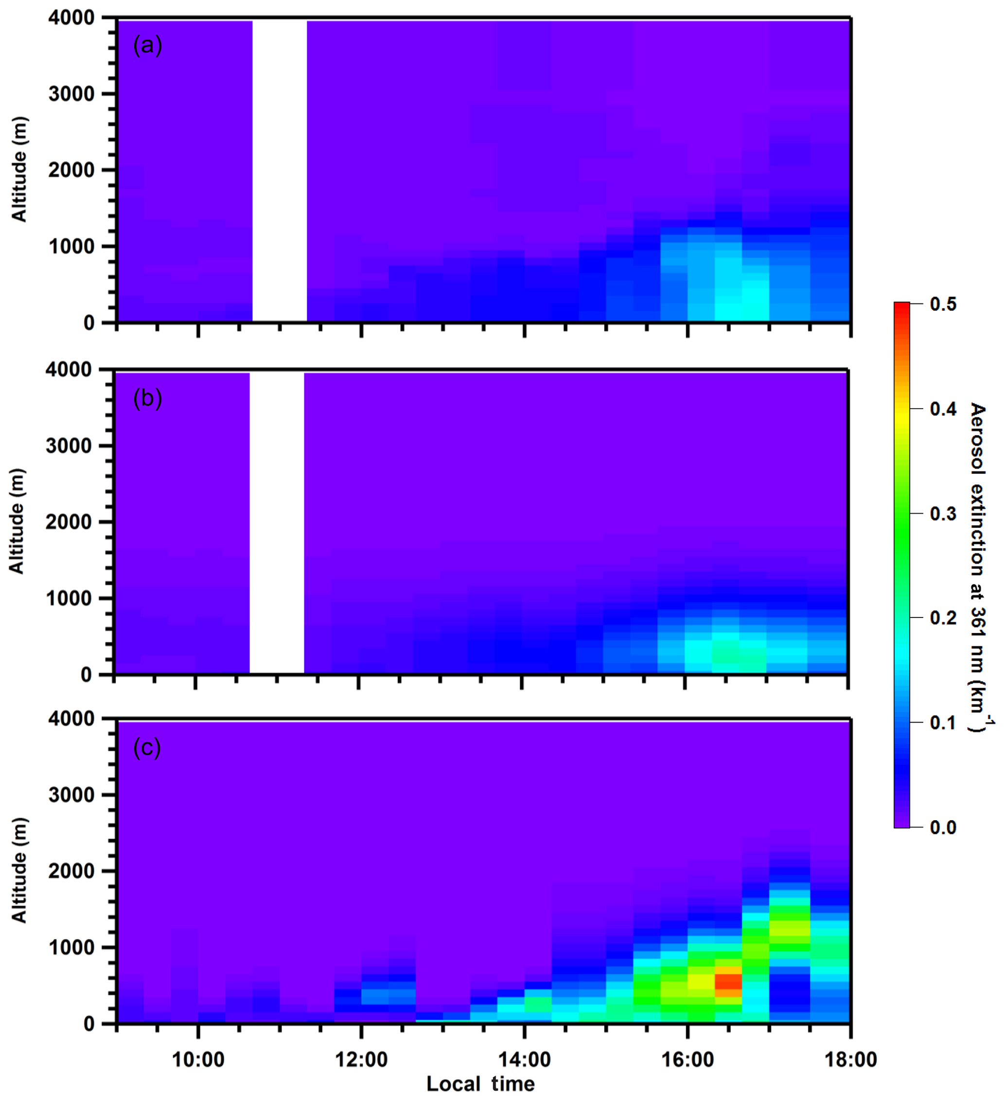
Figure 12The 23 August vertical profiles of aerosol extinction (361 nm) from S ratio of 25 sr: averaged lidar (a), smoothed lidar (b), and MAX-DOAS retrieved measurements (c).
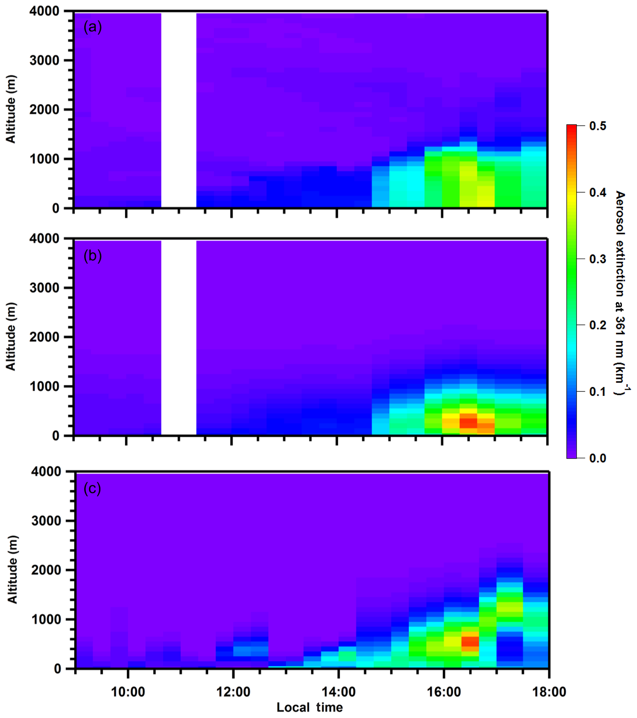
Figure 13The 23 August vertical profiles of aerosol extinction (361 nm) from S ratio of 44 sr within the plume > 14:30 LT: averaged lidar (a), smoothed lidar (b), and MAX-DOAS retrieved measurements (c).
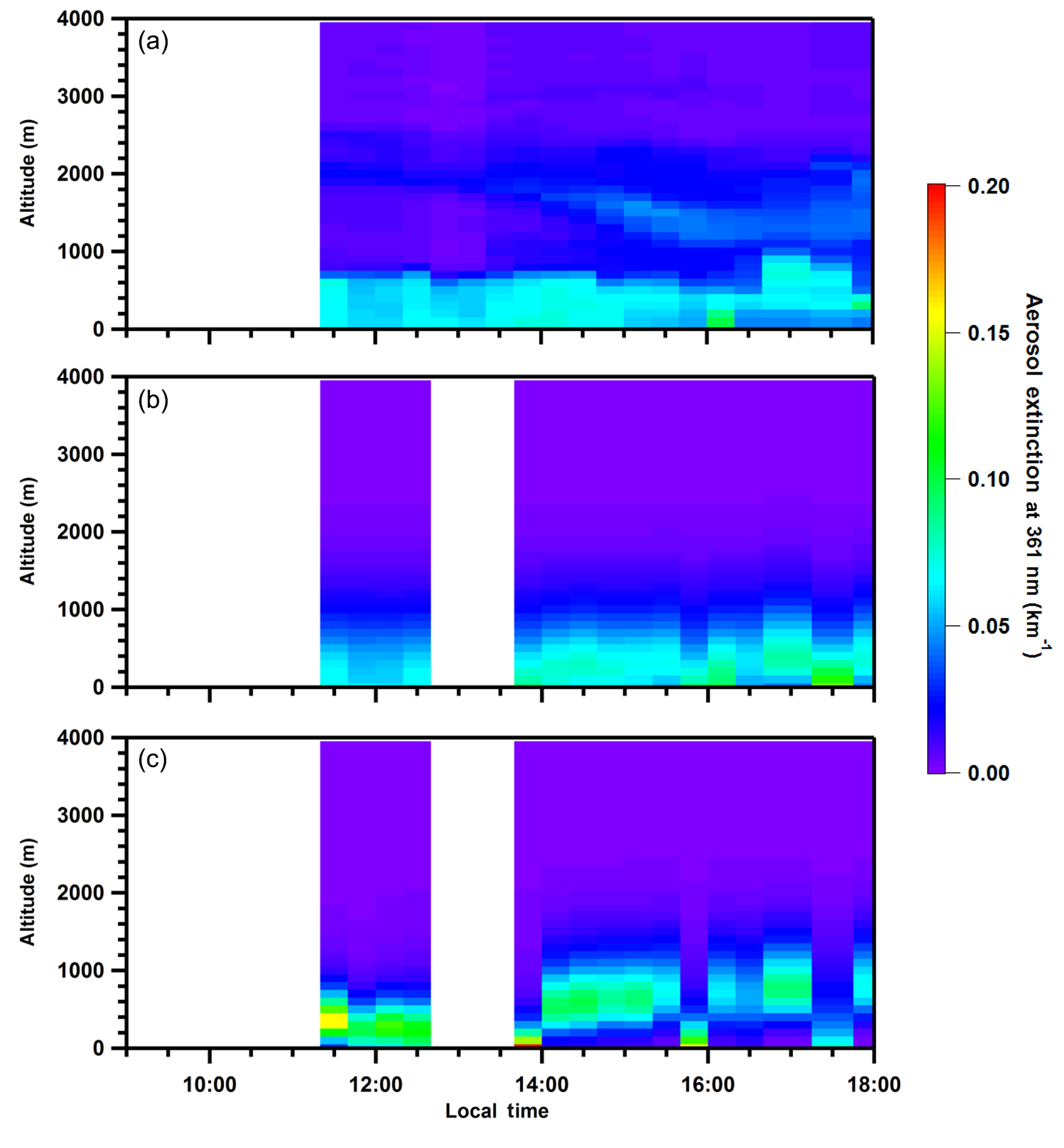
Figure 14The 3 September vertical profiles of aerosol extinction (361 nm) from averaged lidar (a), smoothed lidar (b), and MAX-DOAS retrieved measurements (c).
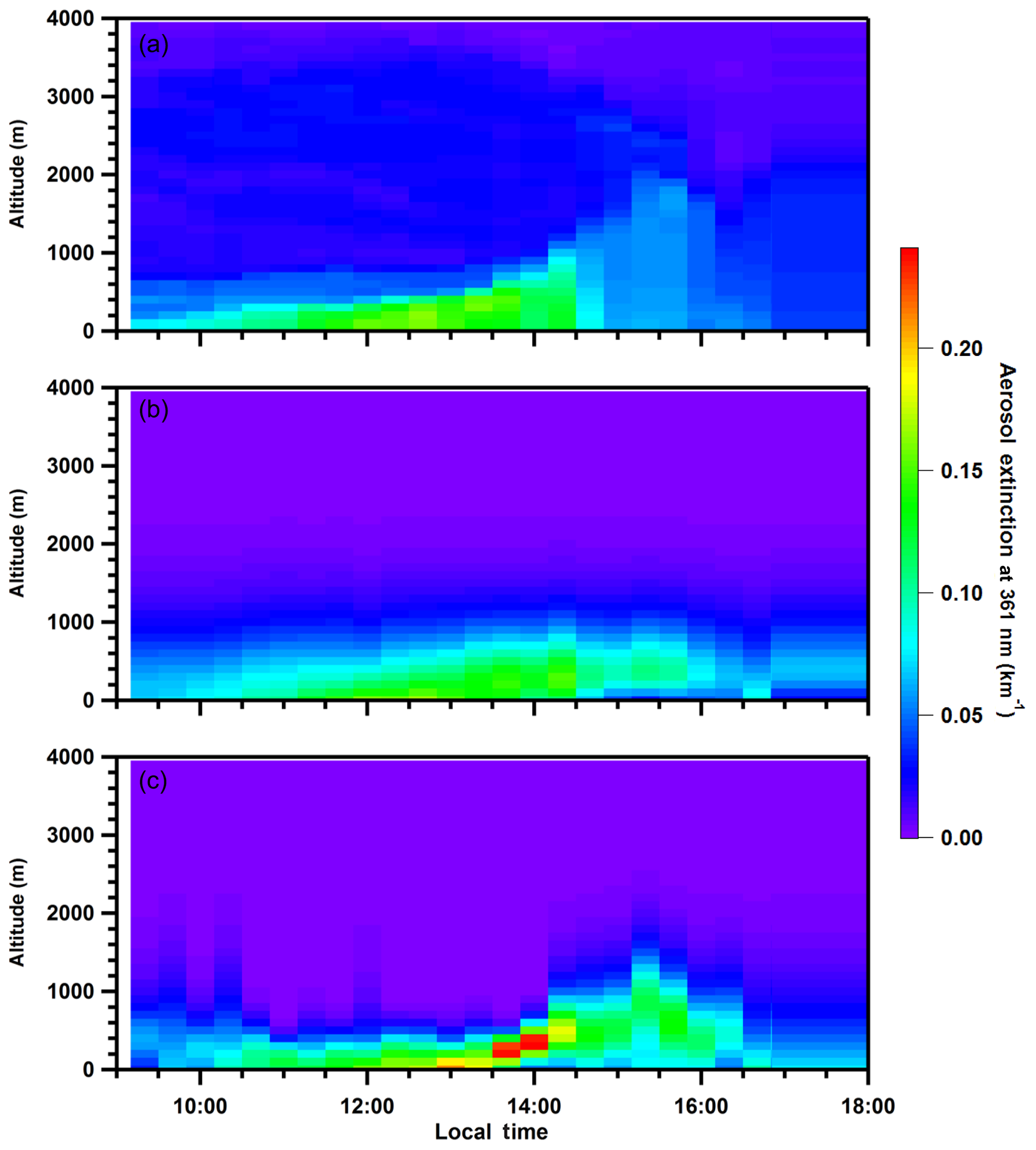
Figure 15The 4 September vertical profiles of aerosol extinction (361 nm) from averaged lidar (a), smoothed lidar (b), and MAX-DOAS retrieved measurements (c).
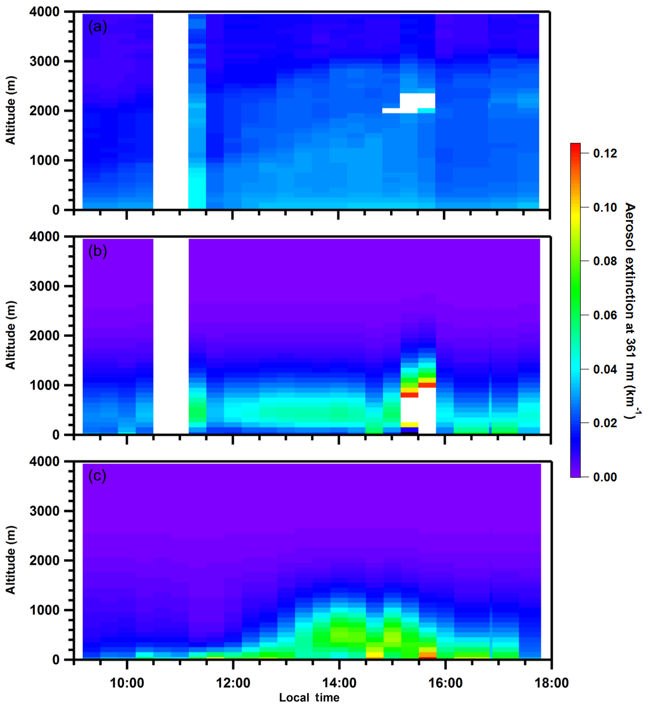
Figure 16The 5 September vertical profiles of aerosol extinction (361 nm) from averaged lidar (a), smoothed lidar (b), and MAX-DOAS retrieved measurements (c). Omitted data in the afternoon were measurements of cirrus clouds.
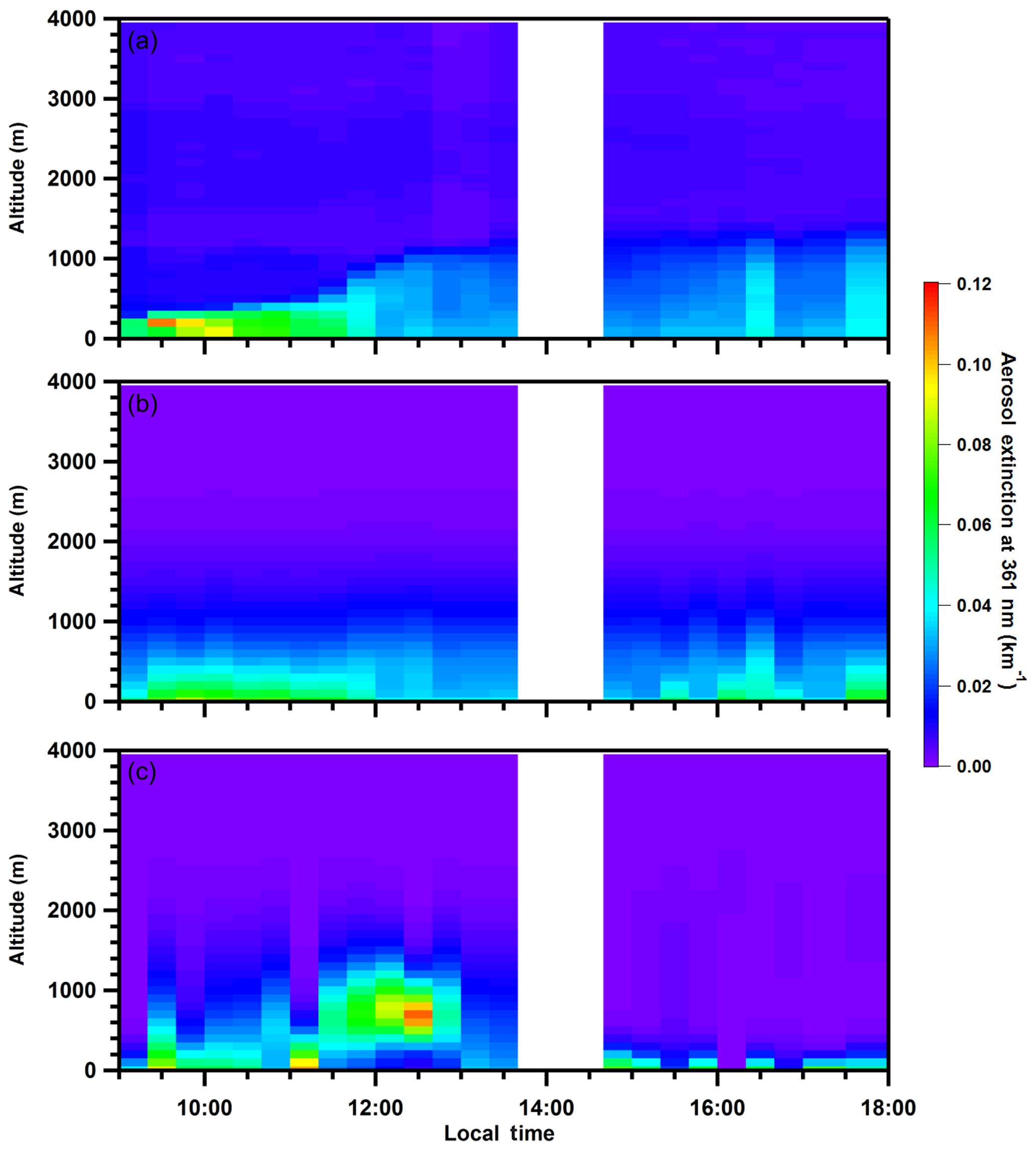
Figure 17The 6 September vertical profiles of aerosol extinction (361 nm) from averaged lidar (a), smoothed lidar (b), and MAX-DOAS retrieved measurements (c).
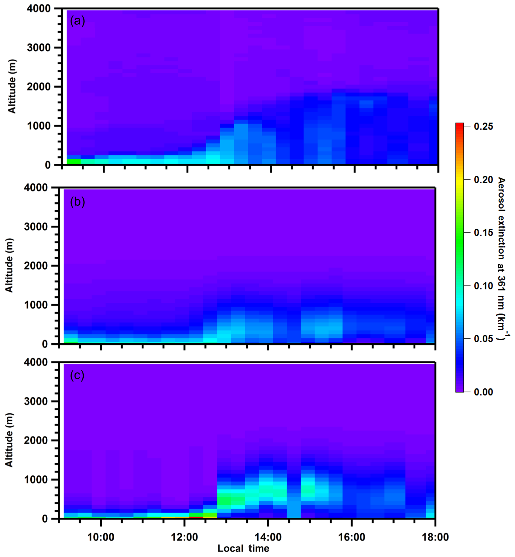
Figure 18The 7 September vertical profiles of aerosol extinction (361 nm) from averaged lidar (a), smoothed lidar (b), and MAX-DOAS retrieved measurements (c).
Smoothing alters the shape and magnitude of the averaged lidar profiles in several ways. Smoothing the averaged lidar profiles generally “compresses” the profiles by vertically attributing extinction at higher altitudes to lower altitudes (compare a and b in Figs. 12–18). This result is expected due to the decreasing sensitivity of the MAX-DOAS retrieval with increasing altitude apparent in the averaging kernels (Fig. S7). The smoothing also replaces lidar aerosol extinction above ∼1.5 km a.g.l. with the (small) a priori extinction values because the MAX-DOAS measurements have little information content at high altitudes (Fig. S7). This effect is apparent when comparing the 3 September averaged and smoothed lidar profiles above 1.5 km a.g.l. (Fig. 14). Profiles that were relatively uniform within a few hundred metres of the surface can sometimes be smoothed into apparently elevated profiles because the averaging kernel attributes much of the extinction from altitudes aloft to one altitude bin closer to the surface. For example, the averaging kernels for the 4 September 14:10 LT retrieval for altitudes 0.55 to 1.25 km peak at 0.45 km rather than at their respective height (Figs. S7 and S8). Conversely, the smoothing can transform vertically narrow and distinctly elevated profiles near the surface into exponentially decreasing profiles due to the limited vertical resolution of the retrieval (see the 09:30 LT profile in Fig. 17). Therefore, interpretation of the retrieved MAX-DOAS profiles must account for the effects of smoothing on the true atmospheric profiles.
On 23 August, the MAX-DOAS and smoothed lidar vertical profiles (S ratio =25 sr) exhibited similar temporal trends and vertical enhancements within the boundary layer (Fig. 12). The magnitudes of aerosol extinctions were consistent between the smoothed lidar and MAX-DOAS vertical profiles in the morning, supporting the hypothesis that the S ratio of 25 sr was appropriate for “clean” periods. In contrast, the MAX-DOAS extinctions exceeded the smoothed lidar extinctions in the afternoon (Fig. 12). Using an S ratio of 44 sr within the afternoon plume (discussed in Sect. 3.1.2) resulted in smoothed lidar profiles consistent with the MAX-DOAS profiles (Fig. 13). While temporal trends and overall magnitudes were similar, MAX-DOAS retrievals tended to exhibit more distinctly elevated profiles than the smoothed lidar profiles. The use of a constant S ratio within the plume may have caused the lidar profiles to appear more vertically uniform than the true profiles since S ratios can maximize where extinction peaks (Fig. S6). Also, the MAX-DOAS viewing geometry observed air masses south of the field site, closer to industrial sources, where the vertical profiles may have been less well mixed. Finally, MAX-DOAS measurement errors can be mapped into the retrieved profile, leading to uncertainties, but are probably only important at higher altitudes where the measurements contain little information content. Deviations in the MAX-DOAS profiles from the smoothed lidar profiles after 17:00 LT can be attributed to reduced light levels and the longer retrieval time, reducing signal-to-noise ratio and the probability of the viewed air masses changing significantly within the time required to capture the measurements for the retrieval, respectively.
For the 3, 4, and 7 September (morning) comparisons, the MAX-DOAS retrieved profiles generally captured the same temporal and vertical trends in extinction enhancements as the smoothed lidar profiles, but the lidar extinctions were smaller than the MAX-DOAS extinctions (Figs. 14, 15, 18). The S ratio of 25 sr probably underestimated the true values given the presence of sulfate particles (Fig. 11b, c, f) and enhanced SO2 VCDs (Figs. 5b, 6b, 9b). On 5 September the S ratio of 25 sr is expected to be appropriate due to the clean conditions. The magnitudes of the MAX-DOAS extinctions were unexpectedly greater than the smoothed lidar extinctions but were generally equal within error (Fig. 16). The 6 September MAX-DOAS aerosol retrievals appear noisier than the smoothed lidar profiles (Fig. 17). The elevated plumes present in the MAX-DOAS retrievals but not in the lidar profiles may be related to an increased S ratio due to the impact of plumes from the north (Fig. 8g). On 7 September the MAX-DOAS aerosol extinction profiles were of greater magnitude and different in vertical profile shape compared to the smoothed lidar profiles after 12:00 LT. The deviation can be attributed to significant wind shear and rapid temporal variation in the wind profiles after 12:00 LT (Figs. 2f, 3f). Aerosol extinction magnitudes varied by up to a factor of 5 within 10 min in the afternoon (Fig. S11). These conditions violate two assumptions of the MAX-DOAS retrievals: low horizontal inhomogeneity and that the spectra measured during the retrieval time observed the same air mass. Although the MAX-DOAS retrievals of AOD were consistent with the smoothed lidar AODs, the temporal and vertical resolutions of the MAX-DOAS retrievals were insufficient to retrieve accurate vertical profile shapes. The afternoon MAX-DOAS vertical profile retrievals are, therefore, not expected to represent the true atmospheric state.
3.2 Evaluation of MAX-DOAS trace gas retrievals
3.2.1 Comparison of MAX-DOAS and pandora trace gas VCDs
The MAX-DOAS and Pandora SO2 and NO2 VCDs exhibited similar temporal trends over the 4 d of comparison, except during the afternoon of 7 September (Fig. 4c, d; b, c in Figs. 5, 6 and 9).
On 23 August the MAX-DOAS and Pandora VCDs were strongly correlated (R2>0.80) with linear regression slopes of 1.55±0.07 and 2.20±0.07 for SO2 and NO2 VCDs, respectively (Table S4). Greater trace gas enhancements were also observed near the surface at Fort McKay South compared to Oski-Ôtin through in situ measurements by the Wood Buffalo Environmental Association (WBEA) (Wood Buffalo Environmental Association, 2019) (Fig. S12) with slopes of the linear regressions of 1.42±0.05 (R2=0.91) and 1.93±0.07 (R2=0.61) for SO2 and NO2, respectively (Table S2). The strong correlations between the trace gas measurements between the sites indicate that the same air mass impacted both sites but that a more central (higher-concentration) portion of the plume impacted Fort McKay South or that a significant horizontal dilution of the plume occurred during transport.
The NO2 VCDs had a regression slope greater than that of the in situ NO2 measurements (Table S2). NOx may have been lost at a faster rate near the surface during transport due to deposition to the surface (e.g., the boreal forests). Transport times between the sites were relatively long (∼30 min) on this day due to low wind speeds below 600 m a.g.l. (Fig. 2). NOx is lost through surface deposition and photochemical conversion to HONO and HNO3 (Finlayson-Pitts et al., 2003; Wojtal et al., 2011). HONO might be subsequently released as NO and OH, but the HNO3 loss will be virtually permanent.
On 4 September the MAX-DOAS and Pandora VCDs exhibited similar temporal trends and were often equal within error (Fig. 6b, c). The slopes of the linear correlations of the SO2 and NO2 VCDs were 1.10±0.33 (R2=0.51) and 0.95±0.07 (R2=0.85), respectively (Table S6). The greater variability in SO2 between the sites compared to NO2 is consistent with the in situ data between Fort McKay South and the WBEA Bertha Ganter site (Fort McKay North; 57.189428, −111.640583) with R2=0.7 and 0.92 for SO2 and NO2, respectively (Table S6) (Wood Buffalo Environmental Association, 2019). SO2 plumes are more localized in the AOSR, originating mostly from large industrial stacks and fewer sources compared to NO2 (Zhang et al., 2018) (Tables S1, S2). Note that when MAX-DOAS SO2 VCDs were significantly greater than Pandora SO2 VCDs around noon, the SO2 mixing ratios at Fort McKay South were approximately double those at the Bertha Ganter (Fort McKay) site (Fig. S12). These results suggest that the MAX-DOAS performed well in retrieving accurate VCDs of SO2 despite the weaker linear correlation with the Pandora VCDs. The two sites appear to have largely experienced the same air masses within a small temporal period (<20 min), due to higher wind speeds relative to 23 August and 3 September (Fig. 2a, c). Higher wind speeds likely reduced the maximum enhancements in trace gas VCDs compared to 23 August and 3 September due to greater dispersion. Wind shear on 4 September (Fig. 3c) may also have transported only certain altitudes of the elevated plumes from south of Fort McKay South to the sites. In contrast, wind shear on 23 August was limited within 500 m a.g.l. (Fig. 3a).
On 3 and 7 September, the MAX-DOAS and Pandora VCDs demonstrated weak linear correlations (R2<0.2) (Tables S5 and S9).
The 3 September VCD correlations are inconclusive due to the limited number of data points and relatively little variation in the Pandora VCDs. The MAX-DOAS VCDs tended to be higher than the Pandora VCDs. Unlike on 23 August, an examination of the in situ data between sites is not helpful due to the significant wind shear on 3 September and the presence of elevated plumes. Based on the good agreement between the MAX-DOAS and Pandora VCDs on 4 September with similar VCD magnitudes, the apparent overestimation could be due to different air masses experienced by the two sites.
On 7 September the MAX-DOAS were similar to the Pandora trace gas VCDs before 13:30 LT but were much larger after (Fig. 9b, c). The deviation of the MAX-DOAS VCDs is an expected result given the rapid spatial and temporal variation in the wind profiles (discussed in Sect. 3.1.3). Errors of the trace gas retrievals can be expected to be even greater than the aerosol retrieval errors because the retrieved aerosol profiles were used as forward model parameters in the trace gas retrieval. The afternoon MAX-DOAS trace gas retrievals on 7 September are not expected to represent the true atmospheric state. Note that the strength of correlation between the measured and optimal estimation modelled dSCDs of the trace gases was weaker for the retrievals from 7 September (slopes =0.9 and R2=0.67–0.74) compared to 23 August (slopes =0.99 and R2=0.97–0.98) and 4 September (slopes =0.97–9.88 and R2=0.91–0.98) (Table S11). These statistical results are consistent with the good performance of the trace gas retrievals on 23 August and 4 September compared to relatively poor performance on 7 September.
Inter-comparisons of the Pandora and MAX-DOAS VCDs show that the MAX-DOAS retrievals of trace gas VCDs performed well under low to moderate wind speeds and when vertical profiles of pollution were relatively constant within the retrieval period.
3.2.2 Comparison of MAX-DOAS 0–100 m retrieval with active DOAS mixing ratios
The 0–100 m a.g.l. MAX-DOAS trace gas retrievals are shown with the active DOAS mixing ratios in Figs. 4e, f and 5–9d, e. The MAX-DOAS retrievals generally captured the active DOAS temporal trends but tended to overestimate the magnitudes. The MAX-DOAS retrieval yields an estimate of the average concentration within the 0–100 m layer, which is larger than the surface value in case of uplifted layers. Therefore, in situ near-ground instruments, such as active DOAS, are required when accurate surface mixing ratios are required.
The MAX-DOAS retrievals were most consistent with the active DOAS measurement during the late afternoon of 23 August (Fig. 4e, f). SO2 was at its highest levels and assumed to be relatively well mixed within the boundary layer based on the similarity in the temporal trends in SO2 VCDs and surface mixing ratios (Fig. 4g) and the uniformity of the lidar vertical profiles <1 km a.g.l. (Fig. 13a). The mixing ratios were equal within error during the morning and after 14:00 LT with some differences in the early afternoon that may be due to the different viewing geometry. On days other than 23 August, the uncertainty in the surface retrieval is often too high for reliable comparison when the near-surface when SO2 and NO2 were <20 and <10 ppb, respectively. Overall, the MAX-DOAS retrievals of 0–1000 m performed well, considering the frequently complex vertical profiles observed during the study.
3.2.3 Temporal trends of MAX-DOAS Trace gas VCDs and active DOAS mixing ratios
Active DOAS mixing ratios are shown with MAX-DOAS VCDs in Fig. 4g, h and in Figs. 5–9f, g. The VCDs and mixing ratios exhibited similar temporal trends on 23 August and 4–6 September (Figs. 4g, h; 6 and 7f, g) but not on 3 and 7 September (f, g in Figs. 5 and 9). The similar temporal trends in VCDs and mixing ratios observed on 23 August are consistent with the limited vertical wind shear and low to moderate wind speeds, as discussed previously. In contrast, the ratio of VCDs to mixing ratios sometimes varied even during short periods on 4 and 6 September. If the boundary layer is well mixed, the active DOAS mixing ratios and MAX-DOAS VCDs are expected to have similar temporal trends during short periods since the boundary layer is expected to be effectively constant. On 4 September, the temporal trends were very similar until ∼ 13:30 LT, when the rapid decrease in trace gas mixing ratios was not reflected in the VCDs (Fig. 6f, g), indicating elevated pollution plumes that are apparent in the lidar measurements (Fig. S7a). These observations are a testament to the ability of MAX-DOAS to observe elevated pollution plumes not detectable at the surface. The differences in the short-term trends in VCDs and mixing ratios are consistent with the wind profile data around 13:30 LT on 4 September, which indicates westerly to northwesterly wind directions <300 m a.g.l. that are expected to result in relatively clean air near the surface (Fig. 3c). Although measurements of the wind profiles above ∼250 m a.g.l. were unavailable, southerly winds aloft are suggested by the trace gas VCDs remaining enhanced until ∼ 15:00 LT. While significant enhancements of trace gas near the surface tend to contribute to enhanced VCDs, the opposite may not always occur: elevated plumes that cause enhanced VCDs may not result in large surface mixing ratios (Fioletov et al., 2016). The observations in this study indicate that elevated enhancements may also result from vertical wind shear. Techniques for estimating emissions from industrial facilities must account for the possibility that different vertical portions of plumes can be transported in different directions. Such complex pollution conditions require pollution monitoring techniques such as MAX-DOAS that can detect elevated pollution plumes. In addition to being able to observe elevated plumes that are under-sampled by in situ, ground instruments, MAX-DOAS can be used to estimate emissions when deployed using the mobile MAX-DOAS technique (Davis et al., 2019).
3.2.4 MAX-DOAS retrievals of vertical profiles of SO2 and NO2
MAX-DOAS retrievals of vertical profiles of SO2 and NO2 are shown in Fig. 19. Unlike the aerosol profiles, co-located measurements of the trace gas vertical profiles were generally not available. The magnitude and vertical location of the pollution were both highly dependent on wind direction and wind shear. The greatest trace gas enhancements occurred under south–south-easterly wind directions (Figs. 3 and 19) where pollution originated from the greatest sources of SO2 and NO2 to the south (Fig. 1; Tables S1, S2). The MAX-DOAS retrievals performed well in terms of the profile shapes expected based on the wind profiles or evidence of elevated plumes. For example, trace gas pollutants in the MAX-DOAS retrievals were confined largely to <200 m on the mornings of 4 and 7 September (Fig. 19c, f) as expected from the wind shear (Fig. 3). The elevated profiles of SO2 on 3 September before noon and during the afternoon of 4 September are consistent with the results discussed previously.
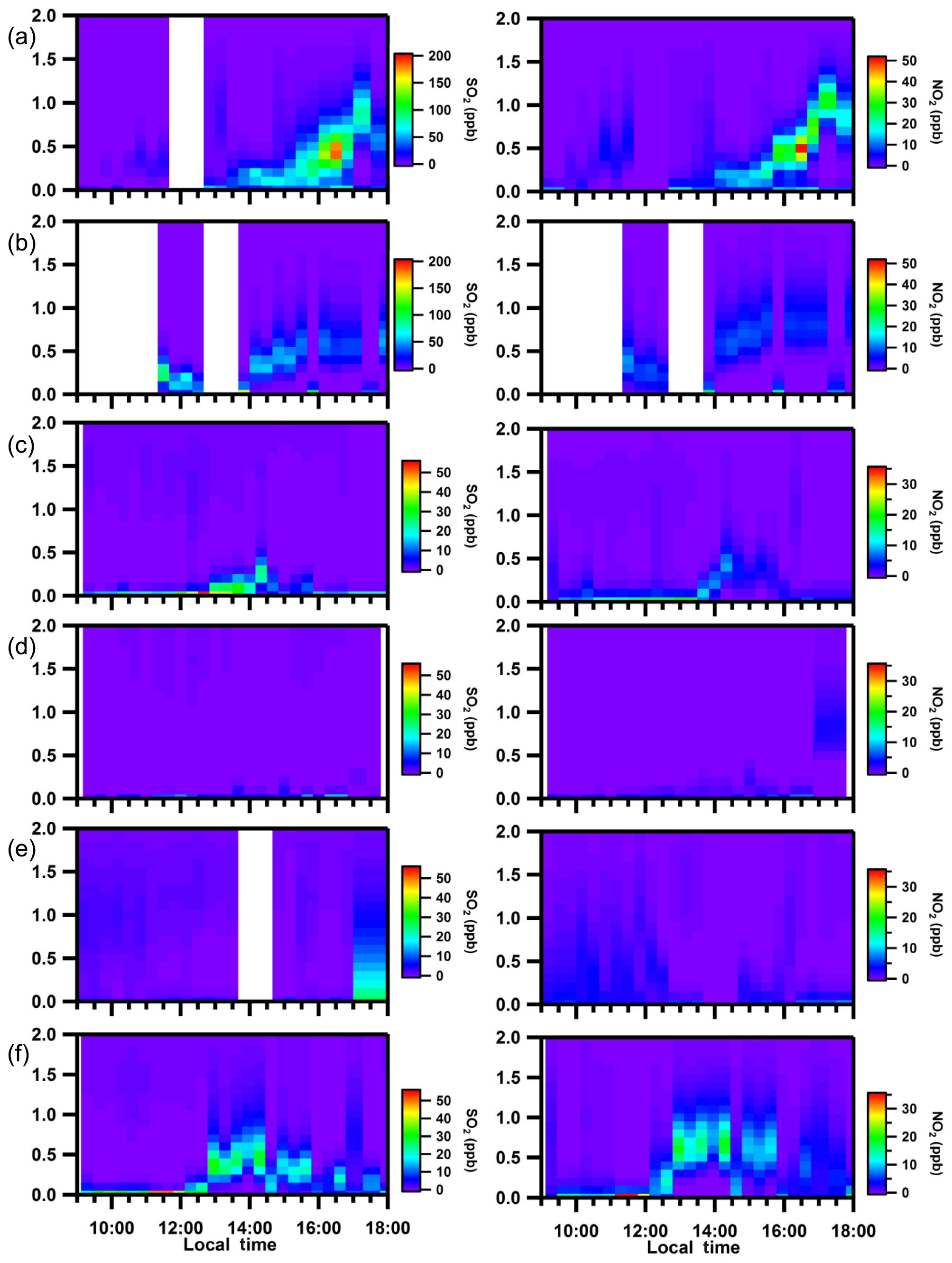
Figure 19MAX-DOAS vertical profiles of SO2 (left column) and NO2 (right column): 23 August (a), 3 September (b), 4 September (c), 5 September (d), 6 September (e), and 7 September (f). Note the different colour scale maximum for 23 August and 3 September.
Aircraft measurements of trace gases on 3 September allow some comparison of the MAX-DOAS retrieved profiles. A vertical profile of SO2 measured during an aircraft spiral ascent at ∼ 14:27 LT in the vicinity of Fort McKay South (Fig. 20) is consistent in magnitude and shape with the MAX-DOAS retrieved vertical profile for 11:00–11:20 LT (Fig. 20). The MAX-DOAS 11:10 LT profile was used for comparison because it appears to have observed the same plume as the aircraft spiral. Although these two profiles cannot be directly compared due to the differences in time and vertical resolutions, the aircraft profile indicates that the magnitudes and elevated shape of the MAX-DOAS profiles of SO2 are reasonable. The elevated SO2 plumes measured by the aircraft and MAX-DOAS could have originated from upgrader stacks at either the Syncrude or Suncor facilities south of Fort McKay South. The aircraft also passed over Fort McKay South at 16:32 LT, measuring 30 ppb of SO2 and 5 ppb of NO2 at 395 m a.g.l. The MAX-DOAS retrieval for 16:20–16:40 LT had maximum SO2 values of 57(±19) ppb at 350 m and maximum NO2 values of 10(±5) ppb at 650 m. Note that the active DOAS measured 20(±0.1) ppb of SO2 and 4.3(±0.1) ppb of NO2 near the surface. These measurements, therefore, suggest that elevated plumes were present and that the MAX-DOAS retrieved magnitudes are reasonable.
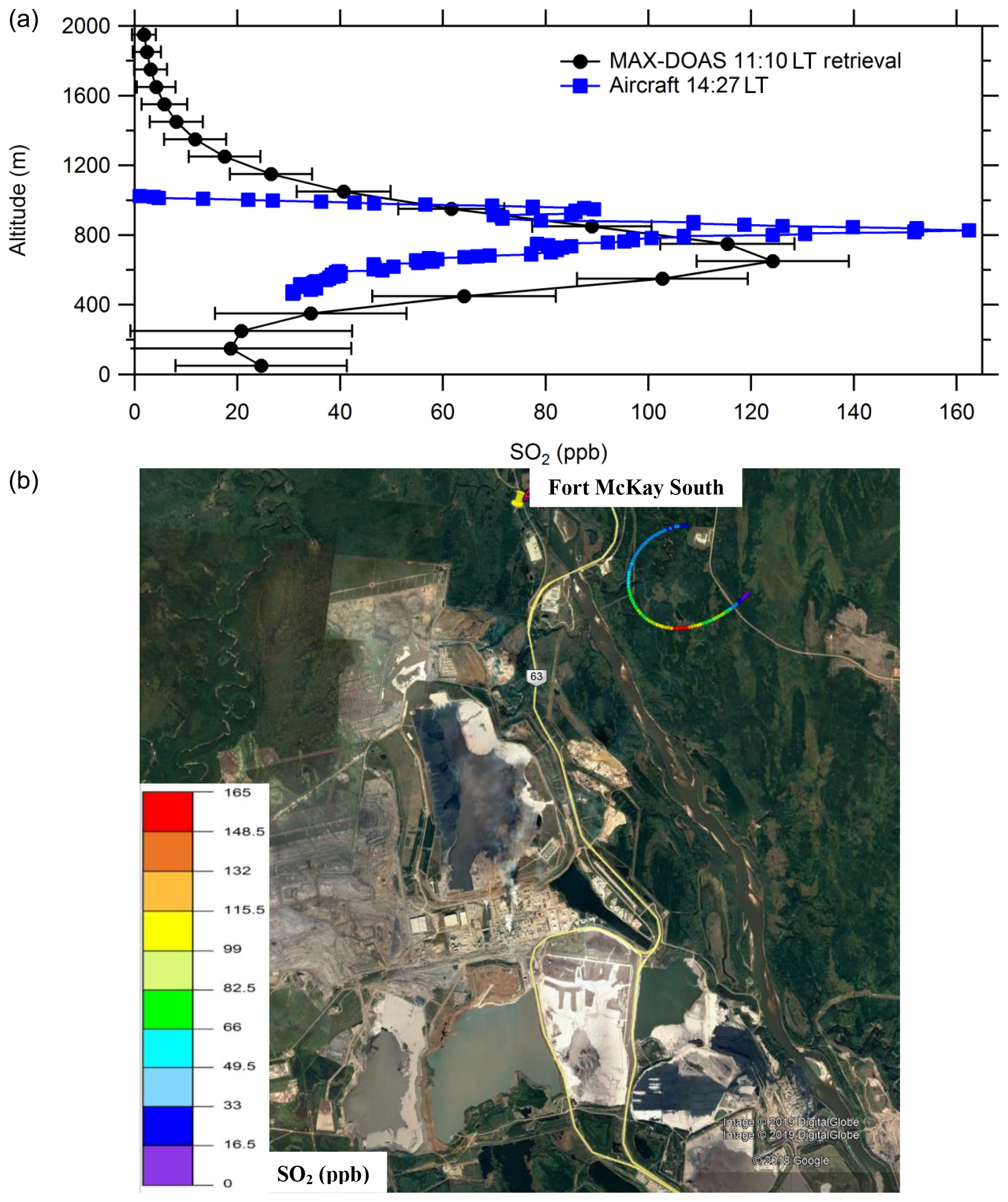
Figure 20The 3 September vertical profiles of SO2 (ppb) from an aircraft spiral measurement (14:26–14:28 LT) and MAX-DOAS retrieved SO2 vertical profile (11:10 LT). Aircraft spiral is shown in a Google Earth plot (b).
3.3 Advantages of MAX-DOAS
MAX-DOAS has an advantage over the zenith lidar technique in detecting aerosol extinction since lidar retrievals cannot detect close to the surface due to challenges with signal overlap (Zieger et al., 2011). Quantifying aerosol extinction from lidar measurements also requires additional knowledge (i.e., the S ratio) (Wagner et al., 2004), as has been highlighted in this paper. The advantage of the MAX-DOAS over the sun photometer (in direct sun viewing mode) is the ability to determine vertical profiles of pollutants versus only total columns. The MAX-DOAS is complementary to active DOAS and other point source measurements when pollution within the boundary layer is vertically inhomogeneous (see Sect. 3.2.3). While surface level local measurements of pollutants are often important for applications such as health exposure studies, they may fail to provide the full picture of the total boundary layer pollution. Such in situ measurements provide highly localized information with little information about elevated plumes that may mix down to the surface downwind. MAX-DOAS allows remote sensing of air masses over longer path-lengths, even if plumes are elevated. The MAX-DOAS method is advantageous over satellite measurements when plumes are localized and can provide more information on near-surface trends.
3.4 Limitations of the inter-comparisons in this study
A limitation to validating the MAX-DOAS AODs against lidar and sun photometer data was the different viewing geometry and slightly different locations. Also, Angstrom exponents used to convert the lidar extinctions to the MAX-DOAS retrieval wavelength would ideally be measured at Fort McKay South. Application of a single S ratio modelled from particle measurements from the near-surface to the entire lidar vertical profile can introduce errors since the S ratio may vary vertically (see Sect. 3.1.2 and Fig. S6). The S ratio can be significantly non-uniform with altitude when the vertical profile is composed of layers of anthropogenic (urban, biomass burning) and/or biogenic aerosols or mixtures of the two. Even if a layer is well mixed, the lidar ratio can change with height if the vertical profile of relative humidity is non-uniform (Weitkamp, 2005).
The MAX-DOAS trace gas VCDs should ideally be compared with a co-located Pandora instrument given the possibility of horizontal inhomogeneity between the sites. Validation of the MAX-DOAS 0–100 m retrieval using the active DOAS mixing ratios was complicated by the lowest viewing elevation angle observing 5 m above the active DOAS light path. The MAX-DOAS “surface” retrieved values are only expected to be equal to the active DOAS values when the air masses were well mixed within 0–100 m a.g.l. A more thorough validation of the MAX-DOAS near-surface retrievals could be achieved with trace gas measurements at multiple heights within 100 m a.g.l. from a tall tower.
In this study, data from a diverse range of instruments have allowed an expansive characterization of the MAX-DOAS retrievals of aerosol extinction, NO2 and SO2. The retrievals performed well when capturing the aerosol loading within the boundary layer. The exception was under conditions of rapid variation in the vertical profiles of pollutants during the retrieval period. The ratio of the MAX-DOAS to sun photometer AODs depended on the vertical location of the aerosol extinction within the atmospheric column. Direct inter-comparisons of AODs between instruments must account for the relative spatial extents observed. The comparison of MAX-DOAS and lidar data combined with S ratio modelling indicated that accurate S ratio values are essential to retrieve accurate profiles of aerosol extinction from lidar measurements when particle composition or size distribution varies significantly temporally or spatially. Direct comparison of MAX-DOAS and lidar AODs should be made with caution when knowledge of the S ratio value(s) is limited. S ratios can be estimated from measurements of particle size distribution and composition using Mie scattering modelling. However, near-surface measurements of particles should only be used to model S ratios when the boundary layer is well mixed. Lidar extinction profiles should ideally be determined using a technique that accounts for the vertical and temporal variation in the S ratio, as in Strawbridge et al. (2018). When the S ratio variability was accounted for, the results of this study indicate that the MAX-DOAS retrievals of aerosol extinction performed well compared to the smoothed lidar results.
Comparisons of averaged and smoothed lidar profiles of aerosol extinction indicated that the vertical sensitivity of the MAX-DOAS retrievals smoothed the true atmospheric profiles towards the surface. This smoothing can transform vertical profiles that are relatively uniform within the boundary layer into apparently elevated profiles and vice versa. This shape change depends on the location of extinction within the true vertical profile and the averaging kernel matrix of the retrieval. Interpretation of the shape of the MAX-DOAS vertical profiles must account for the instrument's sensitivity to the true vertical profile (i.e., the averaging kernel matrix).
MAX-DOAS retrievals of NO2 and SO2 VCDs performed well in comparison to the Pandora VCDs. The exception was when the aerosol retrievals were inaccurate due to rapidly varying vertical profiles. This was an expected result since the aerosol retrievals are used as forward model parameters in the trace gas retrieval. The MAX-DOAS trace gas retrievals within 0–100 m a.g.l. captured the temporal trends observed by the active DOAS measurements, but the MAX-DOAS mixing ratios were statistically greater than the active DOAS values, particularly when SO2 and NO2 were <20 and <10 ppb, respectively. Differences between the instruments' values can be attributed to variability in the trace gas profiles within 150 m a.g.l. The MAX-DOAS observed elevated enhancements of pollution undetected by ground-based techniques such as the active DOAS, which is perhaps its greatest asset. Pollution enhancements at surface level did not always coincide with total boundary layer enhancements and vice versa, due to elevated plumes and/or significant wind shear. The MAX-DOAS vertical profiles of trace gases were consistent with the profiles expected based on the wind direction and shear conditions. Aircraft measurements of SO2 near Fort McKay South on 3 September indicated that the magnitudes and elevated shape of the retrievals were reasonable.
A major advantage of the MAX-DOAS technique is the ability to simultaneously retrieve total columns and vertical profiles of trace gases and aerosol extinction in the boundary layer and the lower troposphere from spectral measurements without requiring knowledge of the aerosol size distributions or compositions. These advantages are important in industrial regions where the vertical profiles of pollutants vary temporally and spatially and in situ monitoring can under-sample plumes. In the AOSR and similar industrial regions, a full understanding of the air quality conditions requires instruments, such as MAX-DOAS, capable of observing the total boundary layer on a horizontal scale of a few kilometres, in addition to traditional in situ instruments.
| Acronym | Expansion |
| a.g.l. | Above ground level |
| AERONET | Aerosol Robotic Network |
| AOD | Aerosol optical depth |
| AOSR | Athabasca oil sands region |
| APS | Aerodynamic particle sizer |
| BrO | Bromine oxide |
| CCD | Charge-coupled device |
| ClO | Chlorine oxide |
| DOAS | Differential optical absorption spectroscopy |
| dSCD | Differential slant column density |
| ECCC | Environment and Climate Change Canada |
| FRS | Fraunhofer reference spectrum |
| HCHO | Formaldehyde |
| Lidar | Light detection and ranging |
| MAX-DOAS | Multi-Axis Differential Optical Absorption Spectroscopy |
| NH3 | Ammonia |
| NO2 | Nitrogen dioxide |
| NO3 | Nitrate radical |
| NOx | Nitrogen oxides (NO2+NO) |
| O4 | Tetraoxygen |
| OH | Hydroxyl radical |
| PM2.5 | Particulate matter with a diameter <2.5 µm |
| ppb | Parts per billion |
| ppt | Parts per trillion |
| RI | Refractive index |
| SMPS | Scanning mobility particle sizer |
| SO2 | Sulfur dioxide |
| SP-AMS | Soot particle aerosol mass spectrometer |
| UV | Ultraviolet |
| VCD | Vertical column density |
| WBEA | Wood Buffalo Environmental Association |
All data used in this study have been published in a publicly available data portal maintained by Environment Canada. The MAX-DOAS, active DOAS, SPAMS, and SMPS data can be found at the following location: ECCC Data (2016a). The sun photometer data and WindRASS data can be found at the following location: ECCC Data (2017). The aircraft SO2 dataset can be found at the following location: ECCC Data (2016b). All datasets are available in *.csv format.
The supplement related to this article is available online at: https://doi.org/10.5194/amt-13-1129-2020-supplement.
ZYWD developed and designed the MAX-DOAS study, performed the investigation, data analysis, and data visualization, and wrote the manuscript and made modifications of the same with contribution from all co-authors. UF supervised and validated the MAX-DOAS data analysis. KBS designed and conducted the ground-based lidar study, including the concept, design, investigation, and data analysis. MA developed the airborne lidar study concept and design and conducted the airborne lidar study investigation and analysis as well as the S ratio modelling. SB analyzed and visualized the SO2 flight data. EGS designed and conducted the SMPS investigation and data analysis. AL conducted the active DOAS investigation and performed the active DOAS data analysis. VEF developed and designed the Pandora study and conducted the investigation and data analysis. IA developed and designed the AERONET AOD study and conducted the investigation and data analysis. CAM conducted the PRATMO modelling for Pandora data analysis and provided the Pandora data. JW supervised the airborne lidar study. MDW and AKYL developed and designed the SP-AMS study concept and conducted the investigation. JB performed the project administration and supervised all studies in the field. JO supervised the SMPS study and the APS data analysis. JO'B developed and designed the SO2 flight data study and conducted the investigation. RS developed and designed the windRASS study concept and conducted the investigation and data analysis. HDO supervised the APS study. CM supervised the APS study. RM supervised the MAX-DOAS study and designed, developed, and supervised the active DOAS study.
The authors declare that they have no conflict of interest.
Funding for this study was provided by Environment and Climate Change Canada and the Canada-Alberta Oil Sands Monitoring program. Zoë Davis, Akshay Lobo and Sabour Baray acknowledge the financial support provided by the Natural Sciences and Engineering Research Council of Canada (NSERC) Collaborative Research and Training Experience Program (CREATE) Integrating Atmospheric Chemistry and Physics from Earth to Space (IACPES).
This research has been supported by the Natural Sciences and Engineering Research Council of Canada (grant nos. RGPIN-2018-05898 and 398061-2011) and Environment Canada (grant no. 583007).
This paper was edited by Robyn Schofield and reviewed by two anonymous referees.
Adams, C., Normand, E. N., McLinden, C. A., Bourassa, A. E., Lloyd, N. D., Degenstein, D. A., Krotkov, N. A., Belmonte Rivas, M., Boersma, K. F., and Eskes, H.: Limb–nadir matching using non-coincident NO2 observations: proof of concept and the OMI-minus-OSIRIS prototype product, Atmos. Meas. Tech., 9, 4103–4122, https://doi.org/10.5194/amt-9-4103-2016, 2016.
Aggarwal, M., Whiteway, J., Seabrook, J., Gray, L., Strawbridge, K., Liu, P., O'Brien, J., Li, S.-M., and McLaren, R.: Airborne lidar measurements of aerosol and ozone above the Canadian oil sands region, Atmos. Meas. Tech., 11, 3829–3849, https://doi.org/10.5194/amt-11-3829-2018, 2018.
Amiri, N., Ghahremaninezhad, R., Rempillo, O., Tokarek, T. W., Odame-Ankrah, C. A., Osthoff, H. D., and Norman, A.-L.: Stable sulfur isotope measurements to trace the fate of SO2 in the Athabasca oil sands region, Atmos. Chem. Phys., 18, 7757–7780, https://doi.org/10.5194/acp-18-7757-2018, 2018.
Baray, S., Darlington, A., Gordon, M., Hayden, K. L., Leithead, A., Li, S.-M., Liu, P. S. K., Mittermeier, R. L., Moussa, S. G., O'Brien, J., Staebler, R., Wolde, M., Worthy, D., and McLaren, R.: Quantification of methane sources in the Athabasca Oil Sands Region of Alberta by aircraft mass balance, Atmos. Chem. Phys., 18, 7361–7378, https://doi.org/10.5194/acp-18-7361-2018, 2018.
Bogumil, K., Orphal, J., Homann, T., Voigt, S., Spietz, P., Fleischmann, O. C., Vogel, A., Hartmann, M., Bovensmann, H., Frerick, J., and Burrows, J. P.: Measurements of molecular absorption spectra with the SCIAMACHY pre-flight model: Instrument characterization and reference data for atmospheric remote sensing in the 230–2380 nm region, J. Photoch. Photobio. A, 157, 167–184, https://doi.org/10.1016/S1010-6030(03)00062-5, 2003.
Bogumil, K., Orphal, J., Homann, T., Voigt, S., Spietz, P., Fleischmann, O. C., Vogel, A., Hartmann, M., Kromminga, H., Bovensmann, H., Frerick, J., and Burrows, J. P.: Measurements of molecular absorption spectra with the SCIAMACHY pre-flight model: instrument characterization and reference data for atmospheric remote-sensing in the 230–2380 nm region, J. Photoch. Photobio. A, 157, 167–184, https://doi.org/10.1016/S1010-6030(03)00062-5, 2003.
Bourgeois, Q., Ekman, A. M. L., Renard, J.-B., Krejci, R., Devasthale, A., Bender, F. A.-M., Riipinen, I., Berthet, G., and Tackett, J. L.: How much of the global aerosol optical depth is found in the boundary layer and free troposphere?, Atmos. Chem. Phys., 18, 7709–7720, https://doi.org/10.5194/acp-18-7709-2018, 2018.
Browaeys, J.: Linear fit with both uncertainties in x and in y, MATLAB Central File Exchange, available at: https://www.mathworks.com/matlabcentral/fileexchange/45711 (last access: 26 February 2019), 2017.
Canadian Council of Ministers of the Environment: Sulphur Dioxide, Sulphur Dioxide, available at: https://www.ccme.ca/en/resources/air/air/sulphur-dioxide.html (last access: 28 May 2019), 2014.
Clémer, K., Van Roozendael, M., Fayt, C., Hendrick, F., Hermans, C., Pinardi, G., Spurr, R., Wang, P., and De Mazière, M.: Multiple wavelength retrieval of tropospheric aerosol optical properties from MAXDOAS measurements in Beijing, Atmos. Meas. Tech., 3, 863–878, https://doi.org/10.5194/amt-3-863-2010, 2010.
Davis, Z. Y. W., Baray, S., McLinden, C. A., Khanbabakhani, A., Fujs, W., Csukat, C., Debosz, J., and McLaren, R.: Estimation of NOx and SO2 emissions from Sarnia, Ontario, using a mobile MAX-DOAS (Multi-AXis Differential Optical Absorption Spectroscopy) and a NOx analyzer, Atmos. Chem. Phys., 19, 13871–13889, https://doi.org/10.5194/acp-19-13871-2019, 2019.
Degenstein, D. A., Bourassa, A. E., Roth, C. Z., and Llewellyn, E. J.: Limb scatter ozone retrieval from 10 to 60 km using a multiplicative algebraic reconstruction technique, Atmos. Chem. Phys., 9, 6521–6529, https://doi.org/10.5194/acp-9-6521-2009, 2009.
Deutschmann, T., Beirle, S., Frieß, U., Grzegorski, M., Kern, C., Kritten, L., Platt, U., Prados-Roman, C., Pukite, J., Wagner, T., Werner, B., and Pfeilsticker, K.: The Monte Carlo atmospheric radiative transfer model McArtim: Introduction and validation of Jacobians and 3D features, J. Quant. Spectrosc. Ra., 112, 1119–1137, https://doi.org/10.1016/j.jqsrt.2010.12.009, 2011.
ECCC: Environment and Climate Change Canada – NPRI Data Search, NPRI Data Search, available at: https://pollution-waste.canada.ca/national-release-inventory/archives/index.cfm?lang=en (last access: 24 April 2019), 2018a.
ECCC: Environment and Climate Change Canada – NPRI Data Search – Facility Search Results, Facil. Search Results – Nitrogen Oxides, available at: https://pollution-waste.canada.ca/national-release-inventory/archives/index.cfm?do=results&lang=en&opt_facility_name=&opt_facility=&opt_npri_id=&opt_report_year=205 (last access: 24 April 2019), 2018b.
ECCC: Environment and Climate Change Canada, NPRI Data Search, Facility Search Results – Sulphur Dioxide, available at: https://pollution-waste.canada.ca/national-release-inventory/archives/index.cfm?do=results&lang=en&opt_facility_name=&opt_facility=&opt_npri_id=&opt_report_year=2017&opt_chemical_type=ALL&opt_industry=&opt_cas_name=7446-09-5&opt_cas_num=&opt_location_type=ALL&opt_province=&opt_postal_code=&opt_community=&opt_csic=&opt_csi2=&15 (last access: 24 April 2019), 2018c.
ECCC Data: Pollutant Transformation, Summer 2013 Ground-based Intensive Multi Parameters – Fort McKay, Oil Sands Region, available at: http://donnees.ec.gc.ca/data/air/monitor/ambient-air-quality-oil-sands-region/pollutant-transformation-summer-2013-ground-based -intensive-multi-parameters-fort-mckay-oil-sands-region/?lang=en (last access: 4 February 2020), 2016a.
ECCC Data: Pollutant Transformation, Summer 2013 Aircraft Intensive Multi Parameters, Oil Sands Region, available at: https://open.canada.ca/data/en/dataset/0bd78f8f-c4da-49c3-9bfd-751e6f300567 (last access: 3 February 2020), 2016b.
ECCC Data: Pollutant Transformation, Ground-based Pollutant Monitoring Multi Parameters – Validated Data – Fort McKay, Oil Sands Region, available at: http://donnees.ec.gc.ca/data/air/monitor/ambient-air-quality-oil-sands-region/pollutant-transformation-ground-based-pollutant-monitoring- multi-parameters-validated-data-fort-mckay-oil-sands-region/?lang=en (last access: 4 February 2020), 2017.
Fenn, M. E., Bytnerowicz, A., Schilling, S. L., and Ross, C. S.: Atmospheric deposition of nitrogen, sulfur and base cations in jack pine stands in the Athabasca Oil Sands Region, Alberta, Canada, Environ. Pollut., 196, 497–510, https://doi.org/10.1016/j.envpol.2014.08.023, 2015.
Finlayson-Pitts, B. J., Wingen, L. M., Sumner, A. L., Syomin, D., and Ramazan, K. A.: The heterogeneous hydrolysis of NO2 in laboratory systems and in outdoor and indoor atmospheres: An integrated mechanism, Phys. Chem. Chem. Phys., 5, 223–242, https://doi.org/10.1039/b208564j, 2003.
Fioletov, V. E., McLinden, C. A., Cede, A., Davies, J., Mihele, C., Netcheva, S., Li, S.-M., and O'Brien, J.: Sulfur dioxide (SO2) vertical column density measurements by Pandora spectrometer over the Canadian oil sands, Atmos. Meas. Tech., 9, 2961–2976, https://doi.org/10.5194/amt-9-2961-2016, 2016.
Frieß, U., Monks, P. S., Remedios, J. J., Rozanov, A., Sinreich, R., Wagner, T., and Platt, U.: MAX-DOAS O4 measurements: A new technique to derive information on atmospheric aerosols: 2. Modeling studies, J. Geophys. Res., 111, D14203, https://doi.org/10.1029/2005JD006618, 2006.
Frieß, U., Deutschmann, T., Gilfedder, B. S., Weller, R., and Platt, U.: Iodine monoxide in the Antarctic snowpack, Atmos. Chem. Phys., 10, 2439–2456, https://doi.org/10.5194/acp-10-2439-2010, 2010.
Frieß, U., Sihler, H., Sander, R., Poehler, D., Yilmaz, S., and Platt, U.: The vertical distribution of BrO and aerosols in the Arctic: Measurements by active and passive differential optical absorption spectroscopy, J. Geophys. Res., 116, D00R04, https://doi.org/10.1029/2011JD015938, 2011.
Frieß, U., Klein Baltink, H., Beirle, S., Clémer, K., Hendrick, F., Henzing, B., Irie, H., de Leeuw, G., Li, A., Moerman, M. M., van Roozendael, M., Shaiganfar, R., Wagner, T., Wang, Y., Xie, P., Yilmaz, S., and Zieger, P.: Intercomparison of aerosol extinction profiles retrieved from MAX-DOAS measurements, Atmos. Meas. Tech., 9, 3205–3222, https://doi.org/10.5194/amt-9-3205-2016, 2016.
Frieß, U., Beirle, S., Alvarado Bonilla, L., Bösch, T., Friedrich, M. M., Hendrick, F., Piters, A., Richter, A., van Roozendael, M., Rozanov, V. V., Spinei, E., Tirpitz, J.-L., Vlemmix, T., Wagner, T., and Wang, Y.: Intercomparison of MAX-DOAS vertical profile retrieval algorithms: studies using synthetic data, Atmos. Meas. Tech., 12, 2155–2181, https://doi.org/10.5194/amt-12-2155-2019, 2019.
Gordon, M., Li, S.-M., Staebler, R., Darlington, A., Hayden, K., O'Brien, J., and Wolde, M.: Determining air pollutant emission rates based on mass balance using airborne measurement data over the Alberta oil sands operations, Atmos. Meas. Tech., 8, 3745–3765, https://doi.org/10.5194/amt-8-3745-2015, 2015.
Gordon, M., Makar, P. A., Staebler, R. M., Zhang, J., Akingunola, A., Gong, W., and Li, S.-M.: A comparison of plume rise algorithms to stack plume measurements in the Athabasca oil sands, Atmos. Chem. Phys., 18, 14695–14714, https://doi.org/10.5194/acp-18-14695-2018, 2018.
Government of Canada: Canadian Environmental Sustainability Indicators – Canada.ca, available at: https://indicators-map.canada.ca/App/CESI_ICDE?keys=AirAmbient_AvgPM&GoCTemplateCulture=en-CA (last access: 6 February 2019), 2018.
Health Canada: Human Health Risk Assessment for Sulphur Dioxide, available at: http://publications.gc.ca/collections/collection_2016/sc-hc/H144-29-2016-eng.pdf (last access: 1 January 2019), 2016.
Hermans, C.: BIRA-IASB Spectroscopy Lab, available at: http://spectrolab.aeronomie.be/index.htm (last access: 27 February 2020), 2011.
Heckel, A., Richter, A., Tarsu, T., Wittrock, F., Hak, C., Pundt, I., Junkermann, W., and Burrows, J. P.: MAX-DOAS measurements of formaldehyde in the Po-Valley, Atmos. Chem. Phys., 5, 909–918, https://doi.org/10.5194/acp-5-909-2005, 2005.
Holloway, A. M. and Wayne, R.: Atmospheric Chemistry, RSC Publishing, Cambridge, UK, 2010.
Hönninger, G. and Platt, U.: Observations of BrO and its vertical distribution during surface ozone depletion at Alert, Atmos. Environ., 36, 2481–2489, https://doi.org/10.1016/S1352-2310(02)00104-8, 2002.
Hönninger, G., von Friedeburg, C., and Platt, U.: Multi axis differential optical absorption spectroscopy (MAX-DOAS), Atmos. Chem. Phys., 4, 231–254, https://doi.org/10.5194/acp-4-231-2004, 2004.
Hsu, Y.-M.: Trends in Passively-Measured Ozone, Nitrogen Dioxide and Sulfur Dioxide Concentrations in the Athabasca Oil Sands Region of Alberta, Canada, Aerosol Air Qual. Res., 13, 1448–1463, https://doi.org/10.4209/aaqr.2012.08.0224, 2013.
Irie, H., Kanaya, Y., Akimoto, H., Iwabuchi, H., Shimizu, A., and Aoki, K.: First retrieval of tropospheric aerosol profiles using MAX-DOAS and comparison with lidar and sky radiometer measurements, Atmos. Chem. Phys., 8, 341–350, https://doi.org/10.5194/acp-8-341-2008, 2008.
Irie, H., Takashima, H., Kanaya, Y., Boersma, K. F., Gast, L., Wittrock, F., Brunner, D., Zhou, Y., and Van Roozendael, M.: Eight-component retrievals from ground-based MAX-DOAS observations, Atmos. Meas. Tech., 4, 1027–1044, https://doi.org/10.5194/amt-4-1027-2011, 2011.
Irie, H., Nakayama, T., Shimizu, A., Yamazaki, A., Nagai, T., Uchiyama, A., Zaizen, Y., Kagamitani, S., and Matsumi, Y.: Evaluation of MAX-DOAS aerosol retrievals by coincident observations using CRDS, lidar, and sky radiometer in Tsukuba, Japan, Atmos. Meas. Tech., 8, 2775–2788, https://doi.org/10.5194/amt-8-2775-2015, 2015.
Jin, J., Ma, J., Lin, W., Zhao, H., Shaiganfar, R., Beirle, S., and Wagner, T.: MAX-DOAS measurements and satellite validation of tropospheric NO2 and SO2 vertical column densities at a rural site of North China, Atmos. Environ., 133, 12–25, https://doi.org/10.1016/j.atmosenv.2016.03.031, 2016.
Keller-Rudek, H., Moortgat, G. K., Sander, R., and Sörensen, R.: The MPI-Mainz UV/VIS Spectral Atlas of Gaseous Molecules of Atmospheric Interest, Earth Syst. Sci. Data, 5, 365–373, https://doi.org/10.5194/essd-5-365-2013, 2013.
Kulmala, M., Vehkamäki, H., Petäjä, T., Dal Maso, M., Lauri, A., Kerminen, V.-M., Birmili, W., and McMurry, P. H.: Formation and growth rates of ultrafine atmospheric particles: a review of observations, J. Aerosol Sci., 35, 143–176, https://doi.org/10.1016/j.jaerosci.2003.10.003, 2004.
Lee, A. K. Y., Adam, M. G., Liggio, J., Li, S.-M., Li, K., Willis, M. D., Abbatt, J. P. D., Tokarek, T. W., Odame-Ankrah, C. A., Osthoff, H. D., Strawbridge, K., and Brook, J. R.: A large contribution of anthropogenic organo-nitrates to secondary organic aerosol in the Alberta oil sands, Atmos. Chem. Phys., 19, 12209–12219, https://doi.org/10.5194/acp-19-12209-2019, 2019.
Levenberg, K.: A method for the solution of certain non-linear problems in least squares, Q. Appl. Math., 2, 164–168, https://doi.org/10.1090/qam/10666, 1944.
Li, X., Brauers, T., Shao, M., Garland, R. M., Wagner, T., Deutschmann, T., and Wahner, A.: MAX-DOAS measurements in southern China: retrieval of aerosol extinctions and validation using ground-based in-situ data, Atmos. Chem. Phys., 10, 2079–2089, https://doi.org/10.5194/acp-10-2079-2010, 2010.
Liggio, J., Li, S.-M., Hayden, K., Taha, Y. M., Stroud, C., Darlington, A., Drollette, B. D., Gordon, M., Lee, P., Liu, P., Leithead, A., Moussa, S. G., Wang, D., O'Brien, J., Mittermeier, R. L., Brook, J. R., Lu, G., Staebler, R. M., Han, Y., Tokarek, T. W., Osthoff, H. D., Makar, P. A., Zhang, J., Plata, D. L. and Gentner, D. R.: Oil sands operations as a large source of secondary organic aerosols, Nature, 534, 91–94, https://doi.org/10.1038/nature17646, 2016.
Liggio, J., Li, S.-M., Staebler, R. M., Hayden, K., Darlington, A., Mittermeier, R. L., O'Brien, J., McLaren, R., Wolde, M., Worthy, D. and Vogel, F.: Measured Canadian oil sands CO2 emissions are higher than estimates made using internationally recommended methods, Nat. Commun., 10, 1863, https://doi.org/10.1038/s41467-019-09714-9, 2019.
Marquardt, D. W.: An algorithm for lesat squares estimation of non-linear parameters, J. Soc. Ind. Appl. Math., 11, 431–441, 1963.
McLaren, R., Wojtal, P., Majonis, D., McCourt, J., Halla, J. D., and Brook, J.: NO3 radical measurements in a polluted marine environment: links to ozone formation, Atmos. Chem. Phys., 10, 4187–4206, https://doi.org/10.5194/acp-10-4187-2010, 2010.
McLaren, R., Wojtal, P., Halla, J. D., Mihele, C. and Brook, J. R.: A survey of NO2:SO2 emission ratios measured in marine vessel plumes in the Strait of Georgia, Atmos. Environ., 46, 655–658, https://doi.org/10.1016/j.atmosenv.2011.10.044, 2012.
McLinden, C. A.: Stratospheric ozone in 3-D models: A simple chemistry and the cross-tropopause flux, J. Geophys. Res., 105, 14653–14665, https://doi.org/10.1029/2000JD900124, 2000.
McLinden, C. A., Fioletov, V., Boersma, K. F., Krotkov, N., Sioris, C. E., Veefkind, J. P., and Yang, K.: Air quality over the Canadian oil sands: A first assessment using satellite observations, Geophys. Res. Lett., 39, L04804, https://doi.org/10.1029/2011GL050273, 2012.
McLinden, C. A., Fioletov, V., Boersma, K. F., Kharol, S. K., Krotkov, N., Lamsal, L., Makar, P. A., Martin, R. V., Veefkind, J. P., and Yang, K.: Improved satellite retrievals of NO2 and SO2 over the Canadian oil sands and comparisons with surface measurements, Atmos. Chem. Phys., 14, 3637–3656, https://doi.org/10.5194/acp-14-3637-2014, 2014.
McLinden, C. A., Fioletov, V., Krotkov, N. A., Li, C., Boersma, K. F. and Adams, C.: A Decade of Change in NO2 and SO2 over the Canadian Oil Sands As Seen from Space, Environ. Sci. Technol., 50, 331–337, https://doi.org/10.1021/acs.est.5b04985, 2016.
Platt, U., Perner, D., and Patz, H.: Simultaneous Measurement of Atmospheric CH2O, O3, and NO2 by Differential Optical-Absorption, J. Geophys. Res., 84, 6329–6335, https://doi.org/10.1029/JC084iC10p06329, 1979.
latt, U. and Stutz, J.: Differential optical absorption spectroscopy: Principles and applications, Springer Verlag, Berlin, Germany, 2008.
Psenner, R.: Environmental impacts on freshwaters: acidifaction as a global problem, Sci. Total Environ., 143, 53–61, https://doi.org/10.1016/0048-9697(94)90532-0, 1994.
Pui, D. Y. H., Chen, S.-C., and Zuo, Z.: PM2.5 in China: Measurements, sources, visibility and health effects, and mitigation, Particuology, 13, 1–26, https://doi.org/10.1016/j.partic.2013.11.001, 2014.
Rodgers, C. D.: Inverse methods for atmospheric sounding: Theory and practice, World Scientific, Singapore, 2000.
Rodgers, C. D. and Connor, B. J.: Intercomparison of remote sounding instruments, J. Geophys. Res., 108, 4116, https://doi.org/10.1029/2002JD002299, 2003.
Rozanov, A., Bovensmann, H., Bracher, A., Hrechanyy, S., Rozanov, V., Sinnhuber, M., Stroh, F., and Burrows, J. P.: NO2 and BrO vertical profile retrieval from SCIAMACHY limb measurements: Sensitivity studies, in: Atmospheric Remote Sensing: Earth's Surface, Troposphere, Stratosphere and Mesosphere – I, edited by: Burrows, J. P. and Eichmann, K. U., Elsevier Science Ltd, Oxford, 36, 846–854, 2005.
Seinfeld, J. H. and Pandis, S. N.: Atmospheric Chemistry and Physics: From Air Pollution to Climate Change, John Wiley & Sons, New York, 2006.
Simpson, I. J., Blake, N. J., Barletta, B., Diskin, G. S., Fuelberg, H. E., Gorham, K., Huey, L. G., Meinardi, S., Rowland, F. S., Vay, S. A., Weinheimer, A. J., Yang, M., and Blake, D. R.: Characterization of trace gases measured over Alberta oil sands mining operations: 76 speciated C2–C10 volatile organic compounds (VOCs), CO2, CH4, CO, NO, NO2, NOy, O3 and SO2, Atmos. Chem. Phys., 10, 11931–11954, https://doi.org/10.5194/acp-10-11931-2010, 2010.
Sioris, C. E., Abboud, I., Fioletov, V. E., and McLinden, C. A.: AEROCAN, the Canadian sub-network of AERONET: Aerosol monitoring and air quality applications, Atmos. Environ., 167, 444–457, https://doi.org/10.1016/j.atmosenv.2017.08.044, 2017.
Strawbridge, K. B.: Developing a portable, autonomous aerosol backscatter lidar for network or remote operations, Atmos. Meas. Tech., 6, 801–816, https://doi.org/10.5194/amt-6-801-2013, 2013.
Strawbridge, K. B., Travis, M. S., Firanski, B. J., Brook, J. R., Staebler, R., and Leblanc, T.: A fully autonomous ozone, aerosol and nighttime water vapor lidar: a synergistic approach to profiling the atmosphere in the Canadian oil sands region, Atmos. Meas. Tech., 11, 6735–6759, https://doi.org/10.5194/amt-11-6735-2018, 2018.
Stutz, J. and Platt, U.: Problems in Using Diode-Arrays for Open Path Doas Measurements of Atmospheric Species, in: Proc. SPIE 1715, Optical Methods in Atmospheric Chemistry, edited by: Schiff H. I. and Platt, U., International Society for Optics and Photonics, SPIE, 329–340, https://doi.org/10.1117/12.140192, 1993.
Tan, W., Liu, C., Wang, S., Xing, C., Su, W., Zhang, C., Xia, C., Liu, H., Cai, Z., and Liu, J.: Tropospheric NO2, SO2, and HCHO over the East China Sea, using ship-based MAX-DOAS observations and comparison with OMI and OMPS satellite data, Atmos. Chem. Phys., 18, 15387–15402, https://doi.org/10.5194/acp-18-15387-2018, 2018.
Tokarek, T. W., Odame-Ankrah, C. A., Huo, J. A., McLaren, R., Lee, A. K. Y., Adam, M. G., Willis, M. D., Abbatt, J. P. D., Mihele, C., Darlington, A., Mittermeier, R. L., Strawbridge, K., Hayden, K. L., Olfert, J. S., Schnitzler, E. G., Brownsey, D. K., Assad, F. V., Wentworth, G. R., Tevlin, A. G., Worthy, D. E. J., Li, S.-M., Liggio, J., Brook, J. R., and Osthoff, H. D.: Principal component analysis of summertime ground site measurements in the Athabasca oil sands with a focus on analytically unresolved intermediate-volatility organic compounds, Atmos. Chem. Phys., 18, 17819–17841, https://doi.org/10.5194/acp-18-17819-2018, 2018.
Wagner, T., von Friedeburg, C., Wenig, M. O., Otten, C., and Platt, U.: UV-visible observations of atmospheric O-4 absorptions using direct moonlight and zenith-scattered sunlight for clear-sky and cloudy sky conditions, J. Geophys. Res., 107, 4424, https://doi.org/10.1029/2001JD001026, 2002.
Wagner, T., Dix, B., von Friedeburg, C., Frieß, U., Sanghavi, S., Sinreich, R., and Platt, U.: MAX-DOAS O4 measurements: A new technique to derive information on atmospheric aerosols – Principles and information content, J. Geophys. Res., 109, D22205, https://doi.org/10.1029/2004JD004904, 2004.
Wagner, T., Deutschmann, T., and Platt, U.: Determination of aerosol properties from MAX-DOAS observations of the Ring effect, Atmos. Meas. Tech., 2, 495–512, https://doi.org/10.5194/amt-2-495-2009, 2009.
Wagner, T., Beirle, S., Brauers, T., Deutschmann, T., Frieß, U., Hak, C., Halla, J. D., Heue, K. P., Junkermann, W., Li, X., Platt, U., and Pundt-Gruber, I.: Inversion of tropospheric profiles of aerosol extinction and HCHO and NO2 mixing ratios from MAX-DOAS observations in Milano during the summer of 2003 and comparison with independent data sets, Atmos. Meas. Tech., 4, 2685–2715, https://doi.org/10.5194/amt-4-2685-2011, 2011.
Wagner, T., Beirle, S., Benavent, N., Bösch, T., Chan, K. L., Donner, S., Dörner, S., Fayt, C., Frieß, U., García-Nieto, D., Gielen, C., González-Bartolome, D., Gomez, L., Hendrick, F., Henzing, B., Jin, J. L., Lampel, J., Ma, J., Mies, K., Navarro, M., Peters, E., Pinardi, G., Puentedura, O., Puḳīte, J., Remmers, J., Richter, A., Saiz-Lopez, A., Shaiganfar, R., Sihler, H., Van Roozendael, M., Wang, Y., and Yela, M.: Is a scaling factor required to obtain closure between measured and modelled atmospheric O4 absorptions? An assessment of uncertainties of measurements and radiative transfer simulations for 2 selected days during the MAD-CAT campaign, Atmos. Meas. Tech., 12, 2745–2817, https://doi.org/10.5194/amt-12-2745-2019, 2019.
Wang, T., Hendrick, F., Wang, P., Tang, G., Clémer, K., Yu, H., Fayt, C., Hermans, C., Gielen, C., Müller, J.-F., Pinardi, G., Theys, N., Brenot, H., and Van Roozendael, M.: Evaluation of tropospheric SO2 retrieved from MAX-DOAS measurements in Xianghe, China, Atmos. Chem. Phys., 14, 11149–11164, https://doi.org/10.5194/acp-14-11149-2014, 2014.
Wang, Y., Beirle, S., Lampel, J., Koukouli, M., De Smedt, I., Theys, N., Li, A., Wu, D., Xie, P., Liu, C., Van Roozendael, M., Stavrakou, T., Müller, J.-F., and Wagner, T.: Validation of OMI, GOME-2A and GOME-2B tropospheric NO2, SO2 and HCHO products using MAX-DOAS observations from 2011 to 2014 in Wuxi, China: investigation of the effects of priori profiles and aerosols on the satellite products, Atmos. Chem. Phys., 17, 5007–5033, https://doi.org/10.5194/acp-17-5007-2017, 2017.
Weitkamp, C.: Lidar: range-resolved optical remote sensing of the atmosphere, Springer Science+Business Media, New York, 2005.
WHO: WHO Air quality guidelines for particulate matter, ozone, nitrogen dioxide and sulfur dioxide, Global update 2005, Summary of Risk Assessment, available at: https://apps.who.int/iris/bitstream/handle/10665/69477/WHO_SDE_PHE_OEH_06.02_eng.pdf?sequence=1 (last access: 18 April 2019), 2006.
Wojtal, P., Halla, J. D., and McLaren, R.: Pseudo steady states of HONO measured in the nocturnal marine boundary layer: a conceptual model for HONO formation on aqueous surfaces, Atmos. Chem. Phys., 11, 3243–3261, https://doi.org/10.5194/acp-11-3243-2011, 2011.
Wood Buffalo Environmental Association: Historical Environmental Monitoring Data, available at: https://wbea.org/historical-monitoring-data/, last access: 29 April 2019.
Wu, F., Xie, P., Li, A., Mou, F., Chen, H., Zhu, Y., Zhu, T., Liu, J., and Liu, W.: Investigations of temporal and spatial distribution of precursors SO2 and NO2 vertical columns in the North China Plain using mobile DOAS, Atmos. Chem. Phys., 18, 1535–1554, https://doi.org/10.5194/acp-18-1535-2018, 2018.
Wu, F. C., Xie, P. H., Li, A., Chan, K. L., Hartl, A., Wang, Y., Si, F. Q., Zeng, Y., Qin, M., Xu, J., Liu, J. G., Liu, W. Q., and Wenig, M.: Observations of SO2 and NO2 by mobile DOAS in the Guangzhou eastern area during the Asian Games 2010, Atmos. Meas. Tech., 6, 2277–2292, https://doi.org/10.5194/amt-6-2277-2013, 2013.
Zhang, J., Moran, M. D., Zheng, Q., Makar, P. A., Baratzadeh, P., Marson, G., Liu, P., and Li, S.-M.: Emissions preparation and analysis for multiscale air quality modeling over the Athabasca Oil Sands Region of Alberta, Canada, Atmos. Chem. Phys., 18, 10459–10481, https://doi.org/10.5194/acp-18-10459-2018, 2018.
Zhao, Y., Duan, L., Xing, J., Larssen, T., Nielsen, C. P., and Hao, J.: Soil Acidification in China: Is Controlling SO2 Emissions Enough?, Environ. Sci. Technol., 43, 8021–8026, https://doi.org/10.1021/es901430n, 2009.
Zhong, S. and Zaveri, R.: Atmospheric Aerosols, in: International Encyclopedia of Geography: People, the Earth, Environment and Technology, edited by: Richardson, D., Castree, N., Goodchild, M. F., Kobayashi, A., Liu, W., and Marston, R. A., John Wiley and Sons, Hoboken, New Jersey, 1–5, https://doi.org/10.1002/9781118786352.wbieg0304, 2017.
Zieger, P., Weingartner, E., Henzing, J., Moerman, M., de Leeuw, G., Mikkilä, J., Ehn, M., Petäjä, T., Clémer, K., van Roozendael, M., Yilmaz, S., Frieß, U., Irie, H., Wagner, T., Shaiganfar, R., Beirle, S., Apituley, A., Wilson, K., and Baltensperger, U.: Comparison of ambient aerosol extinction coefficients obtained from in-situ, MAX-DOAS and LIDAR measurements at Cabauw, Atmos. Chem. Phys., 11, 2603–2624, https://doi.org/10.5194/acp-11-2603-2011, 2011.