Performance evaluation of THz Atmospheric Limb Sounder (TALIS) of China

THz Atmospheric Limb Sounder (TALIS) is a microwave limb sounder being developed for atmospheric vertically resolved profile observations by the National Space Science Center, Chinese Academy of Sciences (NSSC, CAS). It is designed to measure temperature and chemical species such as O₃, HCl, ClO, N₂O, NO, NO₂, HOCl, H₂O, HNO₃, HCN, CO, SO₂, BrO, HO₂, H₂CO, CH₃Cl, CH₃OH, and CH₃CN with a high vertical resolution from about 10 to 100 km to improve our comprehension of atmospheric chemistry and dynamics and to monitor the man-made pollution in the atmosphere. Four heterodyne radiometers including several FFT spectrometers of 2 GHz bandwidth with 2 MHz resolution are employed to obtain the atmospheric thermal emission in broad spectral regions centred near 118, 190, 240, and 643 GHz. A theoretical simulation is performed to estimate the retrieval precision of the main targets and to compare them with that of Aura MLS standard spectrometers. Single scan measurement and averaged measurement are considered in the simulation, respectively. The temperature profile can be obtained with a precision of <2 K for a single scan from 10 to 60 km by using the 118 GHz radiometer, and the 240 and 643 GHz radiometers can provide temperature information in the upper troposphere. Chemical species such as H₂O, O₃, and HCl show a relatively good single scan retrieval precision of <20 % over most of the useful range and ClO, N₂O, and HNO₃ can be retrieved with a precision of <50 %. The other species should be retrieved by using averaged measurements because of the weak intensity and/or low abundance.

1 Introduction

Better precision observation of Earth's atmosphere is essential to numerical weather prediction and climate change studies. Satellites can provide daily global coverage of the atmosphere. Instruments such as nadir microwave sounders and infrared sounders have been applied to measure the atmospheric temperature and humidity but with the poor vertical resolution and altitude range (Swadley et al., 2008). Limb sounders can not only provide the temperature profile with better vertical resolution, but also gather information on chemical composition in a wide altitude range. In the terahertz domain, the measurement performances are independent of the day–night cycle. Microwave limb sounding is a particularly useful technique in detecting stratospheric and mesospheric temperature and chemistry, and also has large potential for global wind measurement in the middle and upper atmosphere (Wu et al., 2008; Baron et al., 2013).

A few instruments have been launched in the last 20 years; their observation data have offered a better understanding of the physical and chemical processes in Earth's atmosphere. The first instrument applying the microwave limb sounding technique from space was the Microwave Limb Sounder (MLS) onboard the Upper Atmosphere Research Satellite (UARS) launched in 1991. The sounder offered unique information of temperature/pressure, O₃, H₂O, ClO, and additional data products including SO₂, HNO₃, and CH₃CN (Waters et al., 1993, 1999; Barath et al., 1993). The Sub-Millimetre Radiometer (SMR) onboard the Odin satellite launched in February 2001 was the first radiometer to employ sub-millimetre limb sounding. Various target species, such as O₃, ClO, N₂O, HNO₃, H₂O, CO, and NO, as well as isotopes of H₂O, O₃, and ice cloud, have been detected (Murtagh et al., 2002; Urban et al., 2005; Eriksson et al., 2007). The Aura MLS, the successor of the UARS MLS onboard the Aura satellite launched in July 2004, gave successful observations of OH, HO₂, H₂O, O₃, HCl, ClO, HOCl, BrO, HNO₃, N₂O, CO, HCN, CH₃CN, SO₂, ice cloud, and wind (Waters et al., 2004, 2006; Wu et al., 2008; Livesey et al., 2013). The Superconducting Submillimeter-wave Limb-Emission Sounder (SMILES) onboard the Japanese Experiment Module (JEM) of the International Space Station (ISS) launched in September 2009 (Kikuchi et al., 2010). SMILES was equipped with 4 K cooled superconductor–insulator–superconductor (SIS) mixers to reduce the system noise temperature, so that the sensitivity of SMILES was higher than that of other similar sensors such as MLS and SMR (Takahashi et al., 2010; Baron et al., 2011). Currently, several new instruments are being developed. Stratospheric Inferred Winds (SIW) is a Swedish mini sub-millimetre limb sounder for measuring wind, temperature, and molecules in the stratosphere. It can provide horizontal wind vectors within 30–90 km, as well as the profiles of temperature, O₃, H₂O, and other trace chemical species (Baron et al., 2018). SIW is designed for small satellites and will be launched as early as 2020–2022. In addition, the successor of SMILES, SMILES-2, is being studied for measuring the whole vertical range of 15–180 km with low noise (Ochiai et al., 2017).

THz Atmospheric Limb Sounder (TALIS) is the pre-research project of civil aerospace technology proposed by the China National Space Administration (CNSA). TALIS is being designed at the National Space Science Center, Chinese Academy of Sciences (NSSC, CAS), for good precision measurement of atmospheric temperature and key chemical species. It has four microwave radiometers in the frequency bands of 118, 190, 240, and 643 GHz, which are similar to the Aura MLS. The TALIS mission objectives are to provide the information for research on the dynamics and the chemistry of the middle and upper atmosphere by measuring the volume mixing ratio (VMR) profile of the chemical species and other atmospheric conditions such as cirrus with much finer spectral resolution. The pre-research will be completed in 2020 and a prototype will be tested. The satellite mission equipped with TALIS will be proposed around 2021.

In this paper, we present a simulation study on precision estimates for the geophysical parameters measured by TALIS. The outline of the present study is as follows: Sect. 2 describes the instrument characteristics and spectral bands. The retrieval method and the simulation result are discussed in Sects. 3 and 4, respectively. The final section gives a conclusion about the performance and future works.

2 Instrument overview

2.1 Instrument characteristics

The TALIS payload (Fig. 1) and its proposed scan characteristics are summarised in Table 1. The instrument will be set at a Sun-synchronous orbit at a normal altitude of 600 km. The offset parabolic antenna is made of a single reflector with a 1.6 m projective aperture and four independent feeds. The layout of four discrete feeds is shown in Fig. 2. Compared with the quasi-optical separation layout (such as MLS), this strategy is easier and has better observation precision since it needs fewer reflectors. But it will lead to a vertical observed displacement of about 20 km between 118, 190, and 643 GHz and a horizontal displacement of 240 GHz. The widths of the field of view (FOV) at the tangent point are about 5.5, 3.8, 3.3, and 0.96 km at 118, 190, 240, and 643 GHz, respectively. The two-point calibration method is adopted by TALIS, and two calibration targets are set at the end of the arm. The extra target can be used to improve the calibration precision and evaluate the antenna effect and non-linearity. At the beginning of the scan, TALIS will view the hot target (ambient temperature) and the extra target (lower temperature) in 3 s, and then it will scan the limb from 0 to 100 km vertically and obtain the spectra every 1 km with an integration time of 0.1 s; finally, it views the cold space at 200 km in 5 s. The process of retrace is the same (also records data) and gives a total period (scan and retrace) of about 36 s.

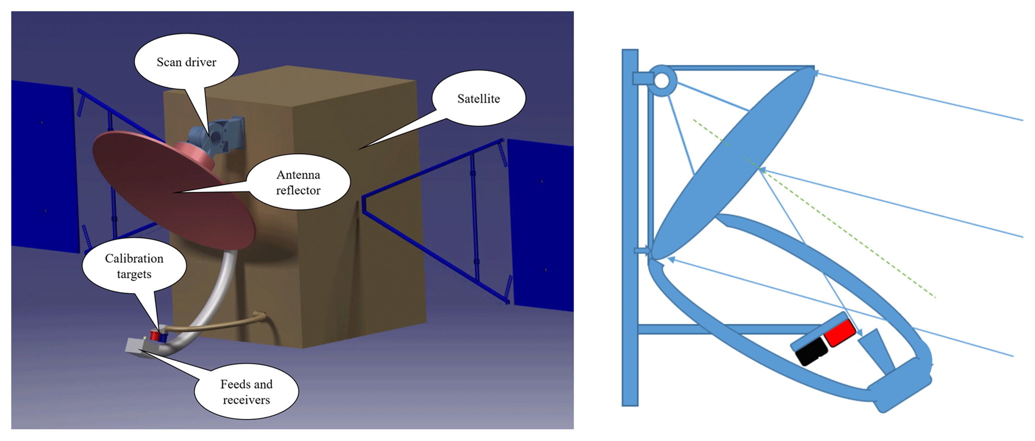
Figure 1 Schematic diagram of the TALIS payload. The reflector, feeds, and receivers are formed into a whole. The scan driver controls the scan angle. The calibration system is fixed in the satellite. At the beginning, the feeds are covered by calibration targets. Then it will scan the limb. When the system rotates to the top, it will view the cold space.

Table 1 Characteristics of the TALIS payload.

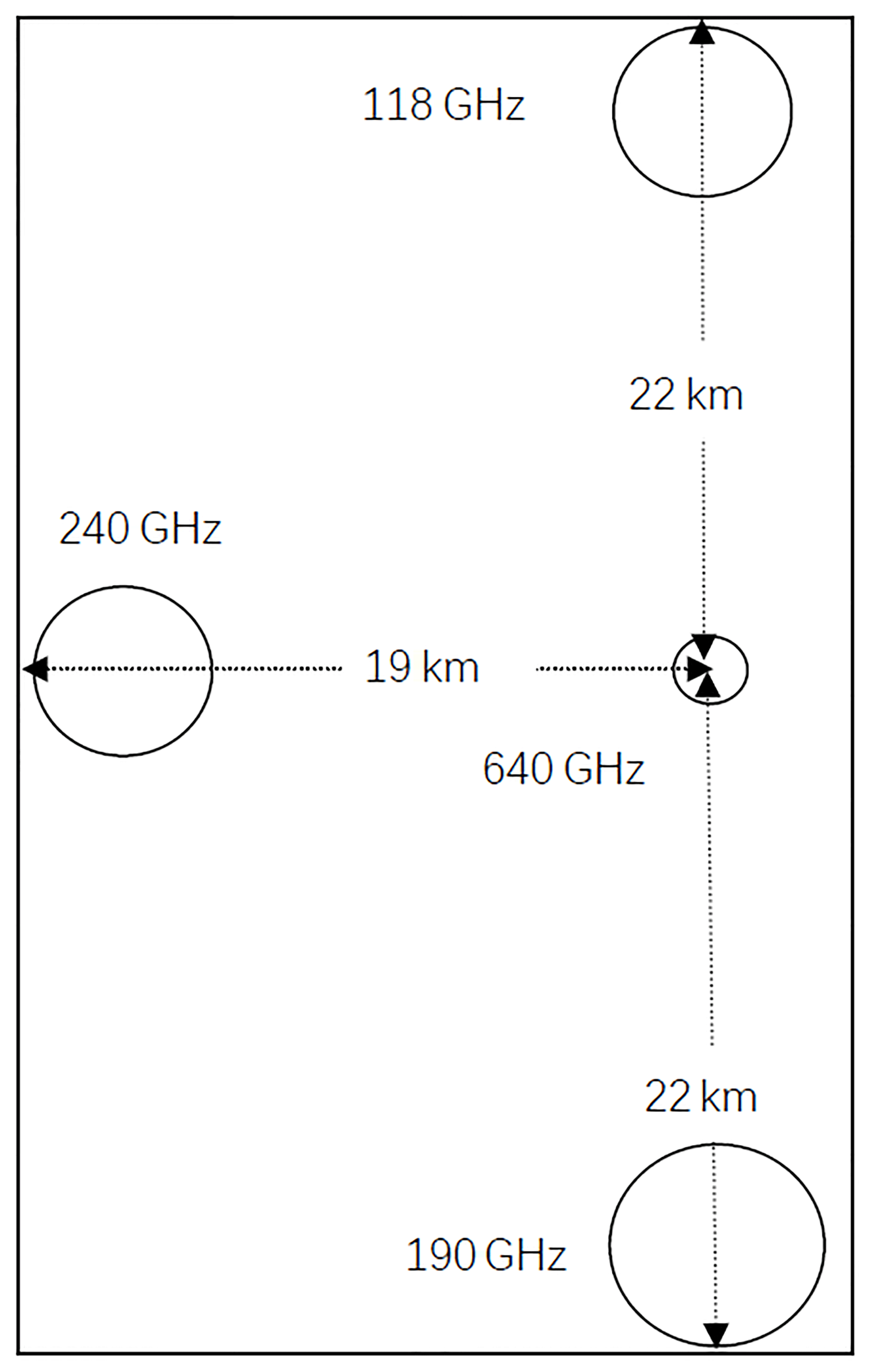
Figure 2 The layout of the four antenna feeds. The observation displacements of the four radiometers are shown.

TALIS has four radiometers which cover the significant thermal emission spectra in the 118, 190, 240, and 643 GHz regions (see Table 2). Single-sideband (SSB) can keep the complete spectral lines, while double-sideband (DSB) can cover more spectral lines because of the image band. Thus, all the radiometers of TALIS will operate in the double-sideband mode except the 118 GHz radiometer. Eleven FFT spectrometers of 2 GHz bandwidth with 2 MHz resolution will be used in TALIS. The bands and system noise temperature for each radiometer are shown in Table 2.

Table 2 Spectral bands and Tsys of TALIS.

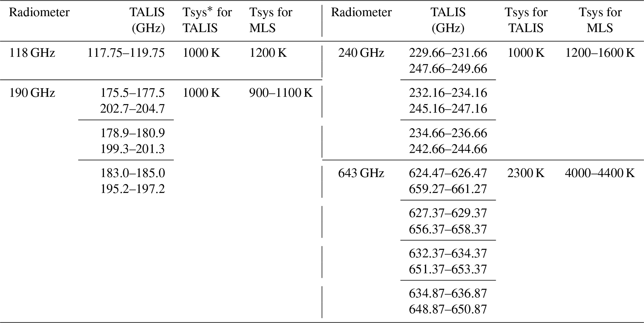
^* This is a single-sideband value for the 118 GHz radiometer, and the double-sideband value is for the other radiometers.

2.2 Spectral bands

The spectral bands of TALIS are selected with the following criteria: (1) maximisation of the number of species which will exert a strong influence on atmospheric chemistry and dynamics, (2) necessary space between the passband, and (3) trade-off between realisable bandwidth and resolution. TALIS covers most spectral bands of the Aura MLS and extends them (see Fig. 3), but lacks the 2.4 THz band. The broader bandwidth and the finer resolution of TALIS can provide a better retrieval precision and effective altitude range compared with the Aura MLS. More chemical species can be measured by TALIS, such as NO₂, NO, and SO₂ (normal concentration).

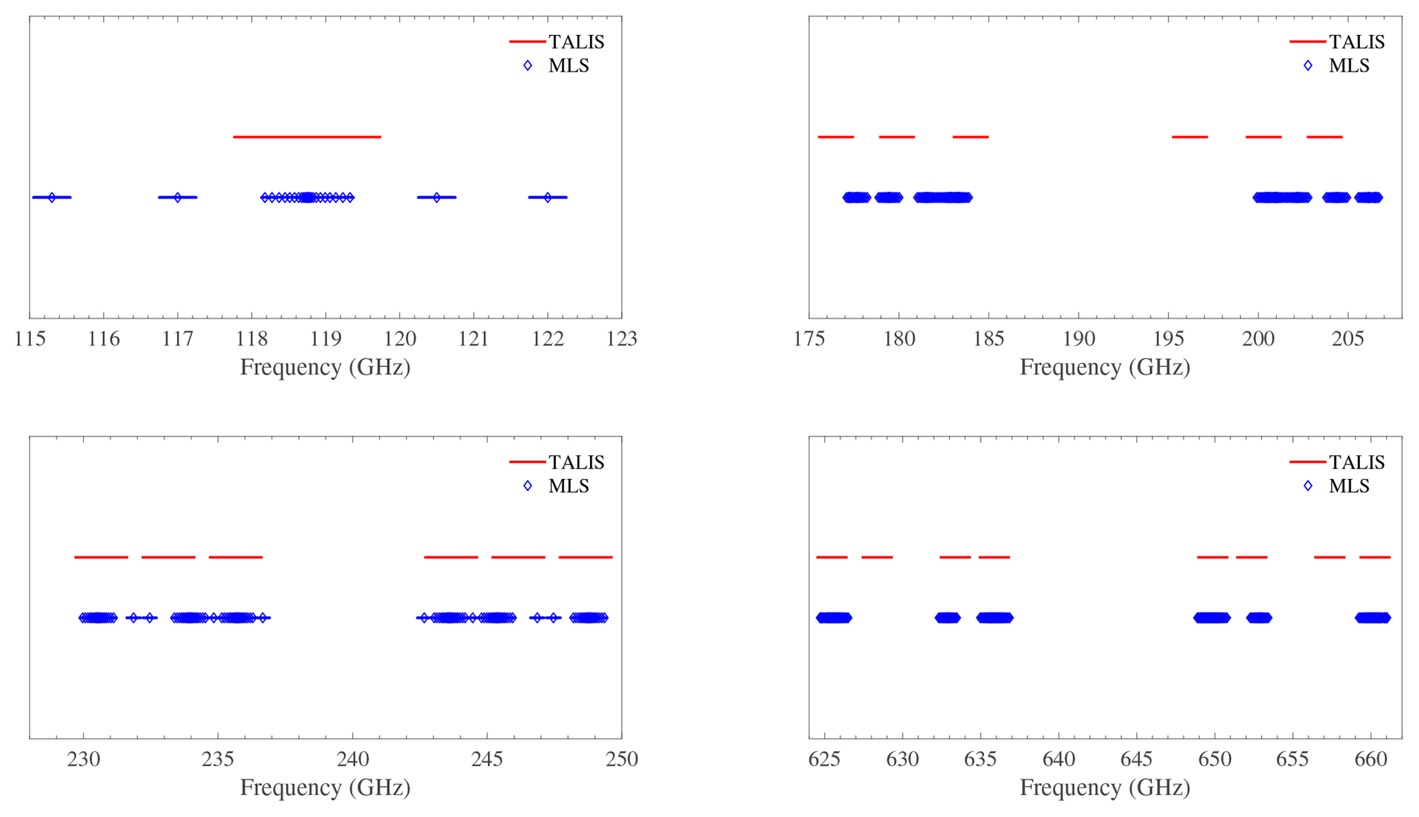
Figure 3 Spectral bands of the Aura MLS and TALIS radiometers. The diamonds represent the filter centres and the solid lines mean the bandwidth of the MLS.

The 118 GHz radiometer, covering the strong O₂ line at 118.75 GHz, is used to measure the atmospheric temperature and tangent pressure. Since there are few meteorological data set about the temperature above the middle atmosphere with good vertical resolution, it is necessary to measure the temperature profile with a wide altitude range, good vertical resolution, and good precision. In addition, the Zeeman effect will affect the O₂ line, and the influence should be studied (Schwartz et al., 2006). Other information such as ice cloud can be treated as an additional measurement. Figure 4 gives an overview of the 118 GHz spectral band.

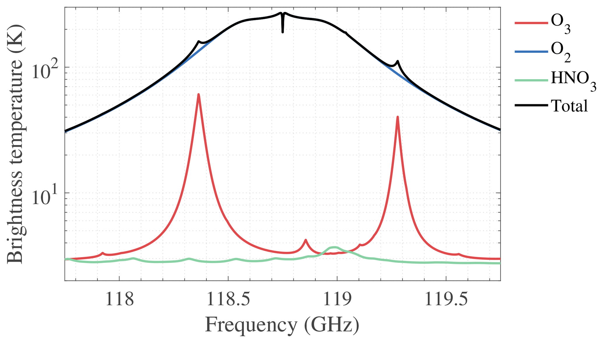
Figure 4 Contributions of the main target chemical species to the 118 GHz spectrum. The brightness temperature is measured from the single-sideband radiometer. The tangent height is 30 km.

The 190 GHz radiometer is mainly designed to cover the 183.31 GHz H₂O line. Monitoring water vapour is important for understanding the mechanisms of humidity feedback on climate and is essential for improving the accuracy of the weather forecast. Other chemical species such as N₂O, ClO, O₃, and HCN are also included in 190 GHz bands (see Fig. 5).

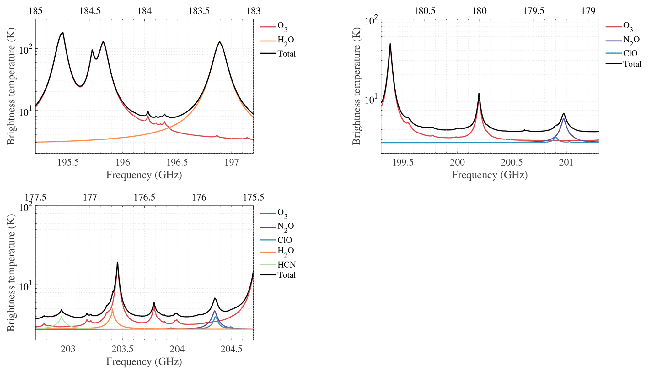
Figure 5 Contributions of the main target chemical species to the 190 GHz spectra. The brightness temperature is measured from the double-sideband radiometer. The tangent height is 30 km. The top axis represents the lower sideband frequencies and the bottom axis represents the upper sideband frequencies. Each panel represents a single spectrometer.

The main objective of the 240 GHz radiometer is to measure the CO at 230.54 GHz, and the strong O₃ lines in a wide spectral band where upper tropospheric O₃ can be obtained with good precision because of the weak water vapour continuum absorption. In addition, the 233.95 GHz O₂ line will be used to measure temperature and tangent pressure together with the 118.75 GHz line. SO₂ is an important pollutant in the Earth' atmosphere and will give rise to acid rain. There is no obvious SO₂ emission with the standard profile present in the passband of the 240 GHz radiometer. The only SO₂ which is observable by the MLS comes from volcanic eruptions. The MLS demonstrated that SO₂ can be measured by 190, 240, and 640 GHz radiometers, but only the 240 GHz SO₂ product is recommended for general use (Pumphrey et al., 2015). The wide and strong lines of HNO₃ can be used to retrieve profiles well. NO₂ is a unique species not covered by the Aura MLS, and TALIS' wider bandwidth and finer resolution have the potential ability to measure it. The spectra of the 240 GHz radiometer are depicted in Fig. 6.

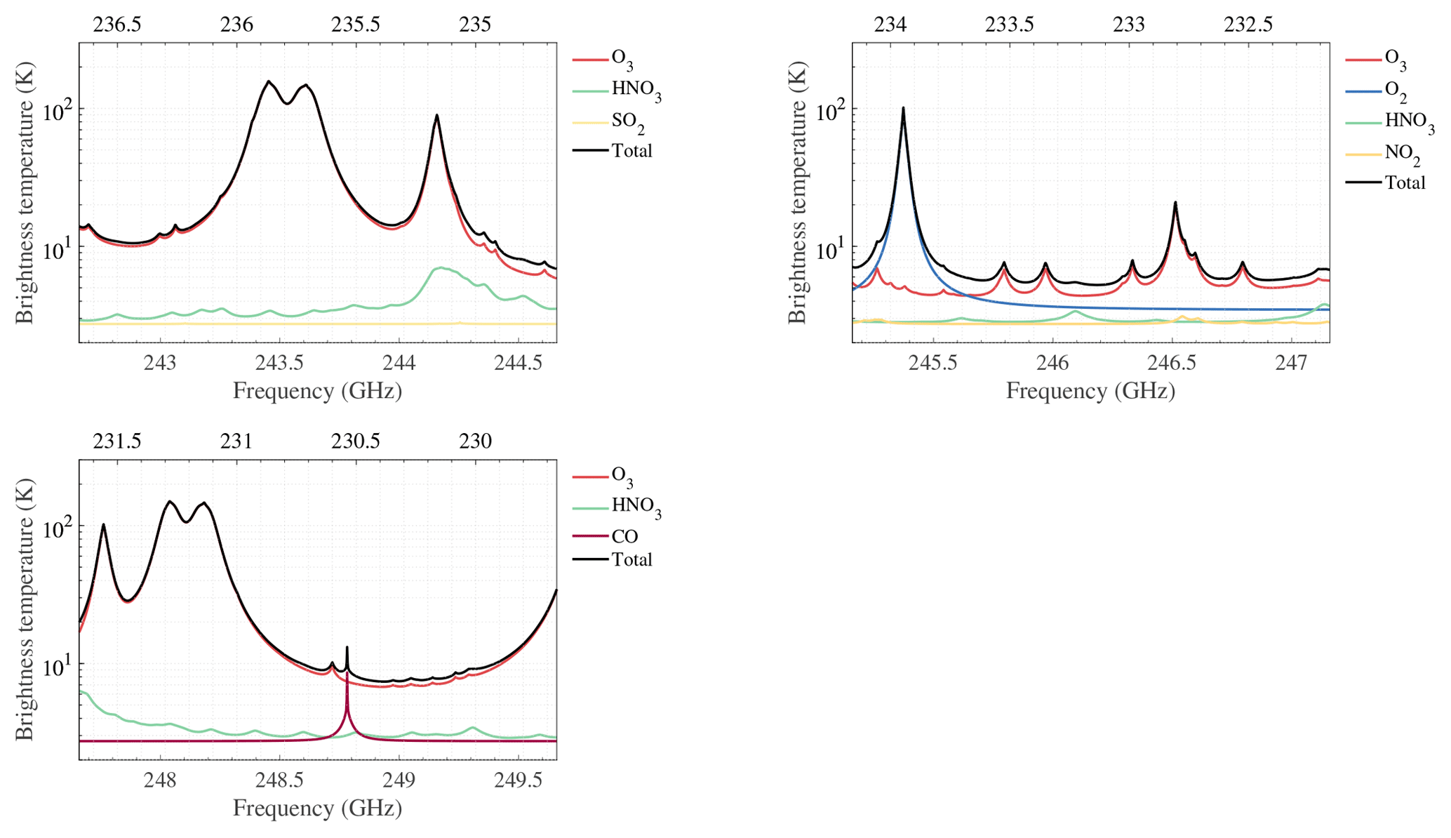
Figure 6 Contributions of the main target chemical species to the 240 GHz spectra. The brightness temperature is measured from the double-sideband radiometer. The tangent height is 30 km. The top axis represents the lower sideband frequencies and the bottom axis represents the upper sideband frequencies. Each panel represents a single spectrometer.

The 643 GHz radiometer is designed to cover as many spectral lines as possible; thus, about 17 species are included. The spectral lines covering O₃, HCl, ClO, N₂O, O₂, and H₂O are clearly visible (Fig. 7), and other lines which are relatively weak such as NO, HNO₃, CO, SO₂, BrO, HO₂, H₂CO, HOCl, and CH₃Cl can also be used. The O₂ line at 627.75 GHz and the H₂O line at 657.9 GHz have the potential to be used as supplements to the 118 and 190 GHz radiometers. O₃ is the major species in the stratosphere and mesosphere, which is quite important in atmospheric radiation transfer. Using the high sensitivity lines in the 643 GHz bands, one can measure O₃ with good precision (Takahashi et al., 2011; Kasai et al., 2013). The only lines of HCl below 1 THz are in the 625 GHz frequency band; thus, HCl can be measured by the 643 GHz radiometer (Lary and Aulov, 2008). ClO is a key catalyst for ozone loss and the 649.45 GHz line is suitable for ClO observation with good precision (Santee et al., 2008; Sato et al., 2012). The HOCl, which will affect the stratospheric chlorine budget, has distinct lines above 600 GHz, and the 635.87 GHz line has been pointed out to be the best line for observation (Urban, 2003). Both the 649.701 and 660.486 GHz lines can be used to measure the hydroperoxyl radical HO₂, which will contribute to the catalytic ozone chemistry in the upper stratosphere and mesosphere (Millán et al., 2015). Since ClO, HO₂, and HOCl all can be measured, the reaction rate of ClO and HO₂ to form HOCl in the atmosphere can be determined (Johnson et al., 1995). N₂O can be measured at 652.834 GHz, which has been validated by the MLS (Lambert et al., 2007). NO has two weak signals at 651.45 and 651.75 GHz, which can be used to measure the abundance. HNO₃ can be measured using the 650 GHz bands. Measuring these nitrogen species will help researchers to understand the chemistry and dynamics of the atmosphere better. The BrO, which plays an important role in the depletion of ozone, can be measured using the 624.768 and 650.179 GHz lines. Because of the low abundance of BrO, measurements must be significantly averaged in order to get reliable results (Millán et al., 2012). CO and H₂CO are the major species in the CH₄ oxidation to CO₂ and H₂O in the stratosphere and mesosphere (Suzuki et al., 2015). The major spectral line of CO used by the MLS is at 230.538 GHz; however, the 661.07 GHz line can also provide information (Livesey et al., 2008). H₂CO has a line at 656.45 GHz, but the signal is very weak. The SO₂ lines in the 660 GHz band have the potential to detect the background levels of SO₂. CH₃Cl can be measured in the 649 GHz band near the line of ClO. The MLS measured CH₃OH and CH₃CN in the troposphere and lower stratosphere by the 625 GHz spectrometer (Pumphrey et al., 2011).

Figure 7 Contributions of the main target chemical species to the 643 GHz spectra. The brightness temperature is measured from the double-sideband radiometer. The tangent height is 30 km. The top axis represents the lower sideband frequencies and the bottom axis represents the upper sideband frequencies. Each panel represents a single spectrometer.

3 Retrieval methodology

3.1 Forward model

The retrieval of data measured by the microwave limb sounder requires the accurate simulation of the observed thermal emission spectra. The forward model is a mathematical tool used to describe the radiative transfer, spectroscopy, and instrumental characteristics. The output of the forward model is the convolution of the atmospheric radiation and instrument response.

Radiative transfer describes the emission, propagation, scattering, and absorption of electromagnetic radiation (Mätzler, 2006). Scattering can usually be neglected above the upper troposphere as the atmosphere is largely cloud-free at these altitudes, and such clouds as there are (e.g. polar stratospheric clouds) have particle sizes shorter than the TALIS observation wavelengths. In this way and assuming local thermodynamic equilibrium (LTE), the formal solution of the radiative transfer equation is defined by

$$\begin{array}{}\text{(1)}& \begin{array}{rl}& I_v\left(S_{\mathrm{2}}\right)=I_v\left(S_{\mathrm{1}}\right)e^{-{\mathit{\tau }}_{v\left(S_{\mathrm{1}},S_{\mathrm{2}}\right)}}\\ & +{\int }_{S_{\mathrm{1}}}^{S_{\mathrm{2}}}{\mathit{\alpha }}_v\left(s\right)B_v\left(T\right)e^{-{\mathit{\tau }}_{v\left(S,S_{\mathrm{2}}\right)}}\mathrm{d}s,\end{array}\end{array}$$

where I_v is the radiance at frequency v reaching the sensor, α is the absorption coefficient, and τ is the opacity or optical thickness. B_v stands for the atmospheric emission which is given by the Planck function describing the radiation of a black body at temperature T and frequency v per unit solid angle, unit frequency interval, and unit emitting surface (Urban et al., 2004):

$$\begin{array}{}\text{(2)}& B_v\left(T\right)={\displaystyle \frac{\mathrm{2}h{v}^{\mathrm{3}}}{c^{\mathrm{2}}}}{\displaystyle \frac{\mathrm{1}}{e^{hv/k_{B}T}-\mathrm{1}}},\end{array}$$

where h is the Planck constant, c is the speed of light, and k_B denotes the Boltzmann constant.

Spectroscopy models and databases allow us to compute the absorption coefficient, which requires pressure, temperature, and the species concentrations along the line of sight. The basic expression can be written as

$$\begin{array}{}\text{(3)}& \mathit{\alpha }\left(v\right)=nS\left(T\right)F\left(v\right),\end{array}$$

where S is called the line strength, F means the line shape function, and n is the number density of the absorber.

Sensor characteristics also have to be taken into account by the forward model, including the antenna field of view, the sideband folding, and the spectrometer channel response (Eriksson et al., 2006).

Firstly, the radiance which encounters the antenna response could be expressed by the integration:

$$\begin{array}{}\text{(4)}& I_v^{\mathrm{a}}={\int }_{\mathrm{\Omega }}{I}_v\left(\mathrm{\Omega }\right)W_v^{\mathrm{a}}\left(\mathrm{\Omega }\right)\mathrm{d}\mathrm{\Omega },\end{array}$$

where $W_v^{\mathrm{a}}$ is the normalised antenna response function. Normally, the variation of I_v in the azimuth angle dimension can be neglected or calculated beforehand. Secondly, a heterodyne mixer converts the signals to intermediate frequency, folding the upper and lower sideband signals together in consequence. The apparent intensity after the mixer can be modelled as

$$\begin{array}{}\text{(5)}& I_v^{\mathrm{if}}={\displaystyle \frac{W_v^{\mathrm{s}}\left(v\right)I_v^{\mathrm{a}}+W_v^{\mathrm{s}}\left(v{}^{\prime }\right)I_{v^{\prime }}^{\mathrm{a}}}{W_v^{\mathrm{s}}\left(v\right)+W_v^{\mathrm{s}}\left(v{}^{\prime }\right)}},\end{array}$$

where $W_v^{\mathrm{s}}$ means the sideband response. At last, the final signal will be recorded by spectrometers, which can be described in a similar way to the antenna response:

$$\begin{array}{}\text{(6)}& I^{\mathrm{c}}={\int }_v{I}_v^{\mathrm{if}}{W}_v^{\mathrm{c}}\left(v\right)\mathrm{d}v.\end{array}$$

Here $W_v^{\mathrm{c}}$ means the normalised channel response, and the radiance is denoted I^c.

The measured radiance is transformed to brightness temperatures using the Planck function.

3.2 Retrieval algorithm

The optimal estimation method (OEM) is the most common method used in atmospheric sounding for retrieving vertical profiles of chemistry species (Rodgers, 2000).

In OEM theory, a predicted noisy measurement $\widehat{y}$ can be expressed by a forward model F with an unknown atmospheric state x and the system noise ϵ_y according to

$$\begin{array}{}\text{(7)}& \widehat{y}=\mathit{F}\left(\mathit{x},\mathit{b}\right)+{\mathit{ϵ}}_y.\end{array}$$

The noiseless predicted radiances F(x,b) are compared with the observed radiance y so that the unknown state which minimises the cost function χ² could be found. The cost function is given by

$$\begin{array}{}\text{(8)}& \begin{array}{rl}& {\mathit{\chi }}^{\mathrm{2}}={\left[y-\mathbf{F}\left(\mathit{x},\mathbf{b}\right)\right]}^T{\mathbf{S}}_y^{-\mathrm{1}}\left[\mathit{y}-\mathbf{F}\left(\mathit{x},\mathit{b}\right)\right]\\ & +{\left[\mathit{x}-{\mathit{x}}_{\mathrm{a}}\right]}^T{\mathbf{S}}_{\mathrm{a}}^{-\mathrm{1}}\left[\mathit{x}-{\mathit{x}}_{\mathrm{a}}\right],\end{array}\end{array}$$

where x_a is an a priori state vector, and S_a and S_y stand for the covariance matrices representing the natural variability of the state vector and the measurement error vector, respectively. Assuming there is no correlation between the channels, the off-diagonal elements of S_y are zero and the diagonal elements are set to the square of the system noise. Usually, a simple formula can be used to determine the SSB radiometric noise standard deviation:

$$\begin{array}{}\text{(9)}& \mathit{ϵ}={\displaystyle \frac{T_{\mathrm{sys}}}{\sqrt{\mathit{\beta }d\mathit{\tau }}}},\end{array}$$

where T_sys is the system noise temperature, which is the sum of the receiver noise temperature and the atmospheric temperature received by the antenna, β is the noise-equivalent bandwidth, and dτ is the integration time for measuring a single spectrum. The diagonal elements of S_a specify a priori variance and the off-diagonal terms are used to describe correlations between adjacent elements in order to make the retrieved profile smoother. The Planck function is used to compute the brightness temperature.

Finally, the Levenberg–Marquardt method, which is the modification of the Gauss–Newton iterative, is used to solve the non-linear problem. The solution is given by

$$\begin{array}{}\text{(10)}& \begin{array}{rl}& {\mathit{x}}_{i+\mathrm{1}}={\mathit{x}}_i+{\left[\left(\mathbf{I}+\mathit{\gamma }\right){\mathbf{S}}_{\mathrm{a}}^{-\mathrm{1}}+{\mathbf{K}}_{\mathrm{xi}}^T{\mathbf{S}}_y^{-\mathrm{1}}{\mathbf{K}}_i\right]}^{-\mathrm{1}}\\ & \left\{{\mathbf{K}}_{\mathrm{xi}}^T{\mathbf{S}}_y^{-\mathrm{1}}\left[\mathit{y}-\mathbf{F}\left({\mathit{x}}_i\right)\right]-{\mathbf{S}}_{\mathrm{a}}^{-\mathrm{1}}\left({\mathit{x}}_i-{\mathit{x}}_{\mathrm{a}}\right)\right\},\end{array}\end{array}$$

where γ denotes the Levenberg–Marquardt parameter and ${\mathbf{K}}_{{\mathrm{x}}_{\mathrm{i}}}$ represents the weighting function matrix (Jacobian). I represents the identity matrix.

The OEM provides an approach to describe the retrieval error completely. The averaging kernel matrix A, which represents the sensitivity of the retrieved state to the true state, is written as

$$\begin{array}{}\text{(11)}& \mathbf{A}={\mathbf{G}}_y{\mathbf{K}}_x={\displaystyle \frac{\partial \widehat{x}}{\partial \mathit{x}}},\end{array}$$

where G_y is the contribution matrix, which expresses the sensitivity of the retrieved state to the measurement:

$$\begin{array}{}\text{(12)}& {\mathbf{G}}_y={\displaystyle \frac{\partial \widehat{x}}{\partial \mathbf{y}}}={\left({\mathbf{K}}_x^T{\mathbf{S}}_y{\mathbf{K}}_x+{\mathbf{S}}_{\mathrm{a}}^{-\mathrm{1}}\right)}^{-\mathrm{1}}{\mathbf{K}}_x^T{\mathbf{S}}_y^{-\mathrm{1}}.\end{array}$$

The retrieval resolution can be estimated from the full width at half maximum (FWHM) of the averaging kernel (Marks and Rodgers, 1993).

There is another useful variable defined as the measurement response, which represents the true state contribution in the retrieval (Baron et al., 2002):

$$\begin{array}{}\text{(13)}& W\left(i\right)={\sum }_j\left|A\left(i,j\right)\right|.\end{array}$$

The ideal measurement response should be near 1. In practice, the reliable range of a retrieval is usually characterised by $\left|W-\mathrm{1}\right|<\mathrm{0.2}$.

Figure 8 The antenna patterns of TALIS.

The retrieval error can be described by two covariance matrices, the smoothing error covariance matrix which is from the need for a priori information,

$$\begin{array}{}\text{(14)}& {\mathbf{S}}_n=\left(\mathbf{A}-\mathbf{I}\right){\mathbf{S}}_{\mathrm{a}}{\left(\mathbf{A}-\mathbf{I}\right)}^T,\end{array}$$

and the measurement error covariance matrix due to the measurement noise,

$$\begin{array}{}\text{(15)}& {\mathbf{S}}_m={\mathbf{G}}_y{\mathbf{S}}_y{\mathbf{G}}_y^T.\end{array}$$

The error covariance matrix used in the following simulation is the total of S_n and S_m.

4 Measurement performance

4.1 Simulation setup

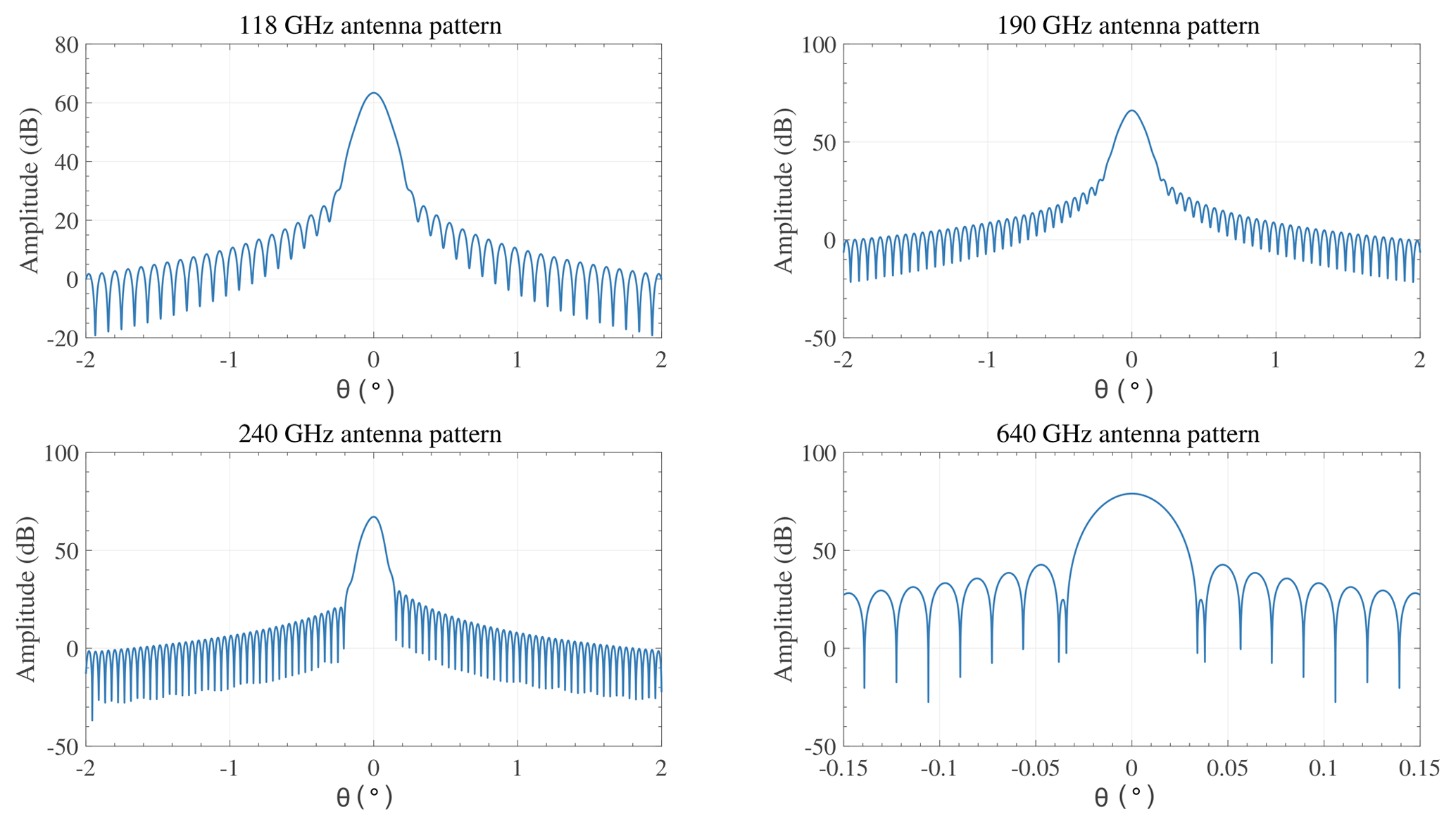
The objective of the simulation is to evaluate the observation performance of TALIS. In this simulation, the Atmospheric Radiative Transfer Simulator (ARTS 2.3) forward model and its corresponding retrieval tool, Qpack2, are used (Eriksson et al., 2005, 2011). The instrumental setup follows the characteristics of TALIS described in Tables 1 and 2. The ideal rectangle back-end channel response function is used. The simulation antenna patterns of the four radiometers are shown in Fig. 8. The full-width at half-power points of antenna patterns are used in the following simulation.

In this simulation, the scan altitude range is from 10 to 90 km and the spectra are obtained every 1 km. A retrieval grid with 2.5 km spacing is used since it can match the FOV of TALIS well, and cutting down the size of the state vector will give a significant increase in speed (Livesey and Van Snyder, 2004). A mid-latitude summer atmospheric condition extracted from FASCOD which is provided by ARTS (profiles of BrO and HO₂ are from MLS L3 v4.2 monthly averaged data, 20–30^∘ N, July 2018) is chosen to perform the simulation (Clough et al., 1986). The scattering from tropospheric clouds, refraction, and the Zeeman effect are not considered because of the large computational complexity. A spectroscopic line parameters catalogue created with the data taken from the JPL catalogue (Pickett et al., 1998), HITRAN database (Rothman et al., 2013), and Perrin catalogue (Perrin et al., 2005) is used for line-by-line absorption calculation. The measurement covariance matrix is set diagonal as described in Sect. 3 in order to reduce the computing time; 110 % of a typical profile is used to build the a priori covariance matrix with 3 km vertical correlation between the adjacent pressure levels by a parametric exponential function. The true profiles are defined with a vertical resolution of 0.5 km. The true species profiles are multiplied by a factor of 1.1 to be the a priori profiles, and to the true temperature profile is added a 5 K offset to be the a priori profile. The molecules are retrieved simultaneously from each band. No spectrally flat extinction term was added.

The expected 1σ noise is calculated by Eq. (9), and the noise is assumed to be 2.2, 2.2, 2.2, and 5.1 K at 118, 190, 240, and 640 GHz, respectively. The species such as BrO and HO₂ whose emission radiances are small compared with the system noise must be averaged to increase the precision. Here the lower noise (1σ noise multiplied by a factor of 0.1, equivalent to a 10^∘ latitude weekly zonal mean) is used to represent the averaged production.

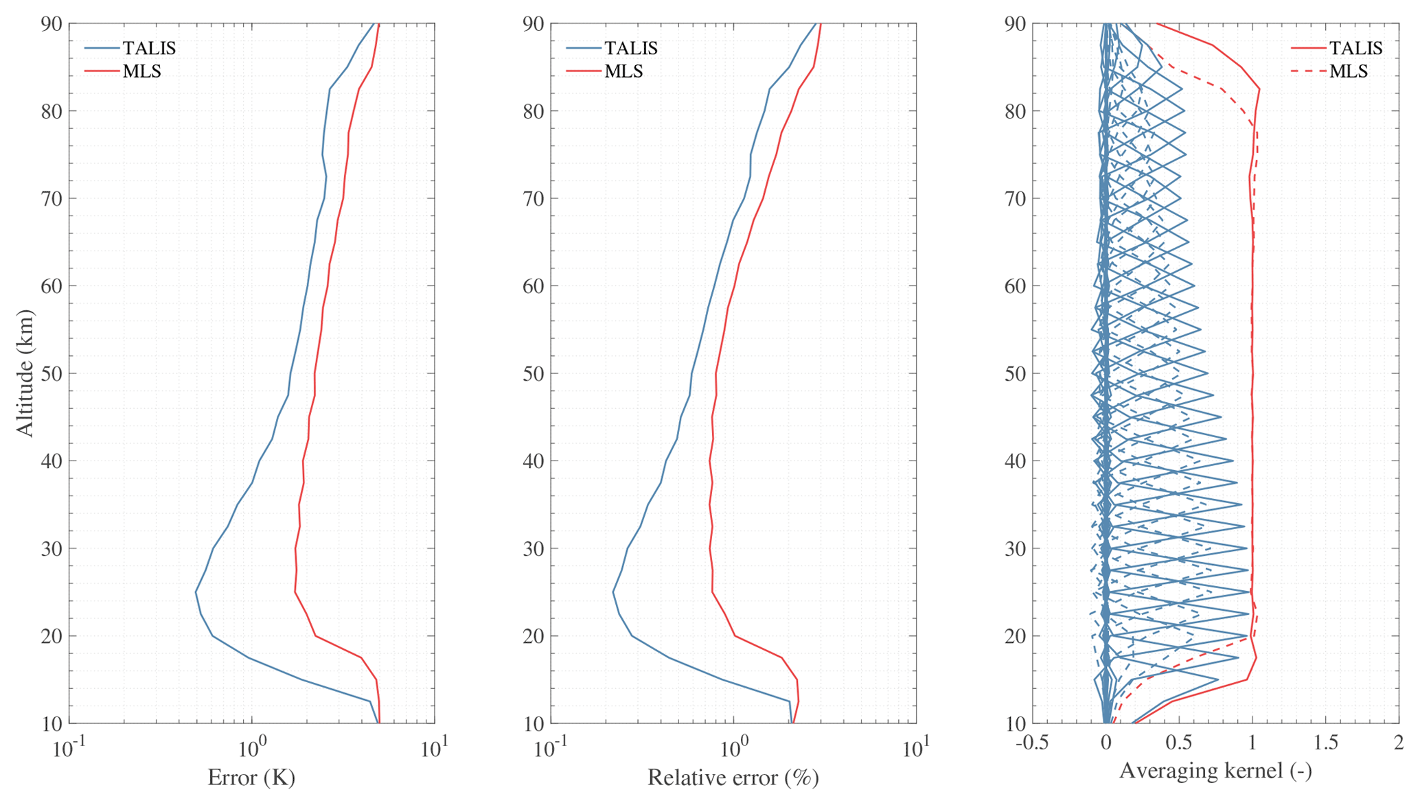
Figure 9 Temperature product comparison between the TALIS FFT spectrometer and the MLS “Standard” spectrometer using the 118.75 GHz line. All other factors are identical.

4.2 Comparison of TALIS and the Aura MLS

As discussed in Sect. 2.2, TALIS has similar bands to the Aura MLS. The major difference between these two instruments is the spectrometers used in limb sounding. A simulation is performed to compare the performance of the main products between the TALIS FFT spectrometer and the Aura MLS “Standard” 25-channel spectrometer. Figures 9 to 11 show the retrieval products of TALIS and MLS; all the factors are identical, except the spectrometer.

Figure 10 H₂O product comparison between the TALIS FFT spectrometer and MLS “Standard” spectrometer using the 183.31 GHz line. All other factors are identical.

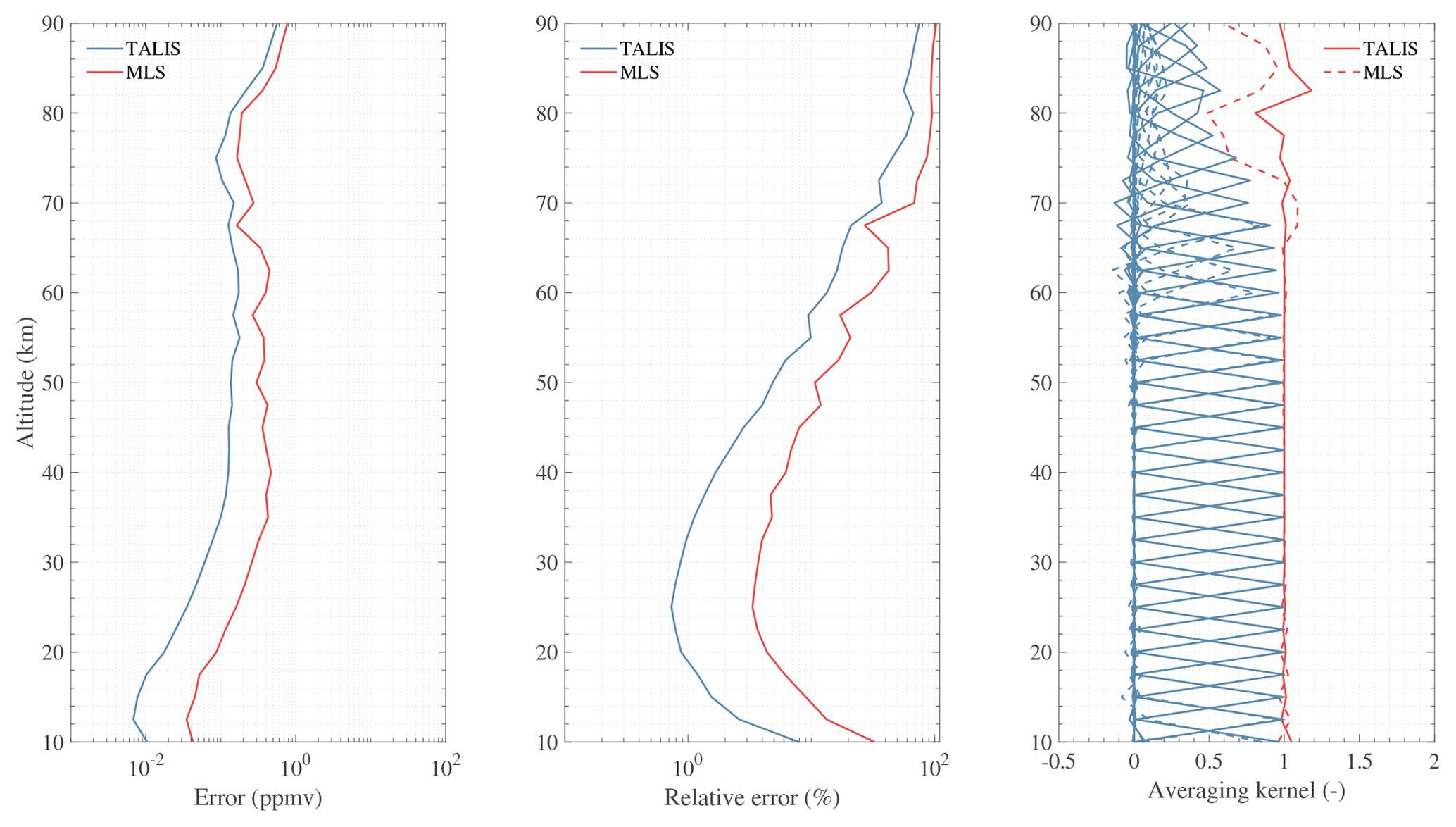
Figure 11 O₃ product comparison between the TALIS FFT spectrometer and MLS “Standard”' spectrometer using the 235.71 GHz line. All other factors are identical.

According to the simulation results, TALIS can do a better job than the Aura MLS because of the wider bandwidth and finer resolution. The temperature precision of TALIS is 1.5 K better than the Aura MLS at about 15–30 km and the vertical resolution is also improved. The difference in precision becomes small above 50 km. H₂O precision is improved by about 2 %–10 % at about 15–50 km. O₃ precision is improved by about 3 %–20 % at about 10–60 km. However, the digital autocorrelator spectrometers of the MLS which can improve the performance in the mesosphere are not considered here.

4.3 Retrieval precision

Since the simulation has been performed, an evaluation of the retrieval precision on the target species of TALIS is made. Results are plotted in Figs. 12 to 28. The precision (square root of diagonal elements of the error covariance matrix) is given for a single scan and averaged measurement, respectively, and the relative error is also provided. Auxiliary information about the averaging kernel function and measurement response are also included. Results are discussed in detail in the following.

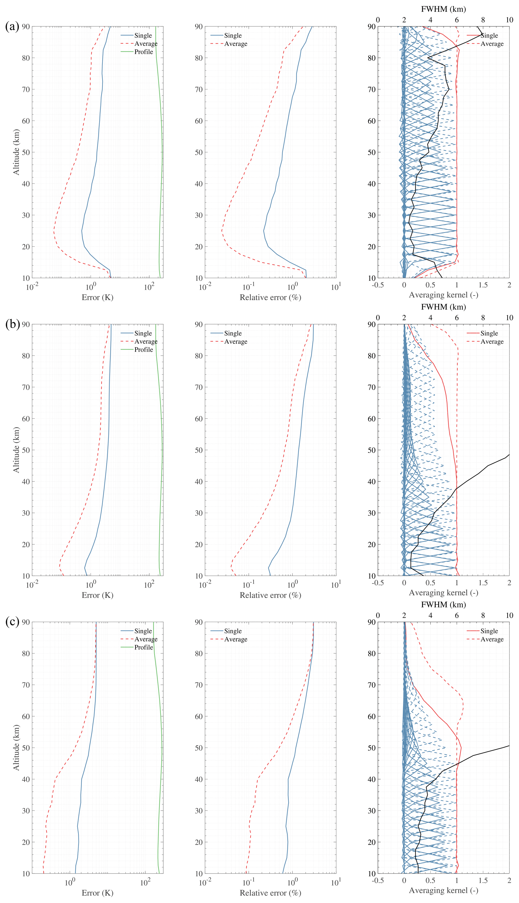
Figure 12 Simulation results of temperature retrieval using 118.75 (a), 233.95 (b), and 627.75 GHz (c) lines. “Single” and “Average” represent the retrieval error using different noise. “Profile” represents the typical profile used in the simulation. The black solid line in the last panel represents the FWHM (i.e. vertical resolution).

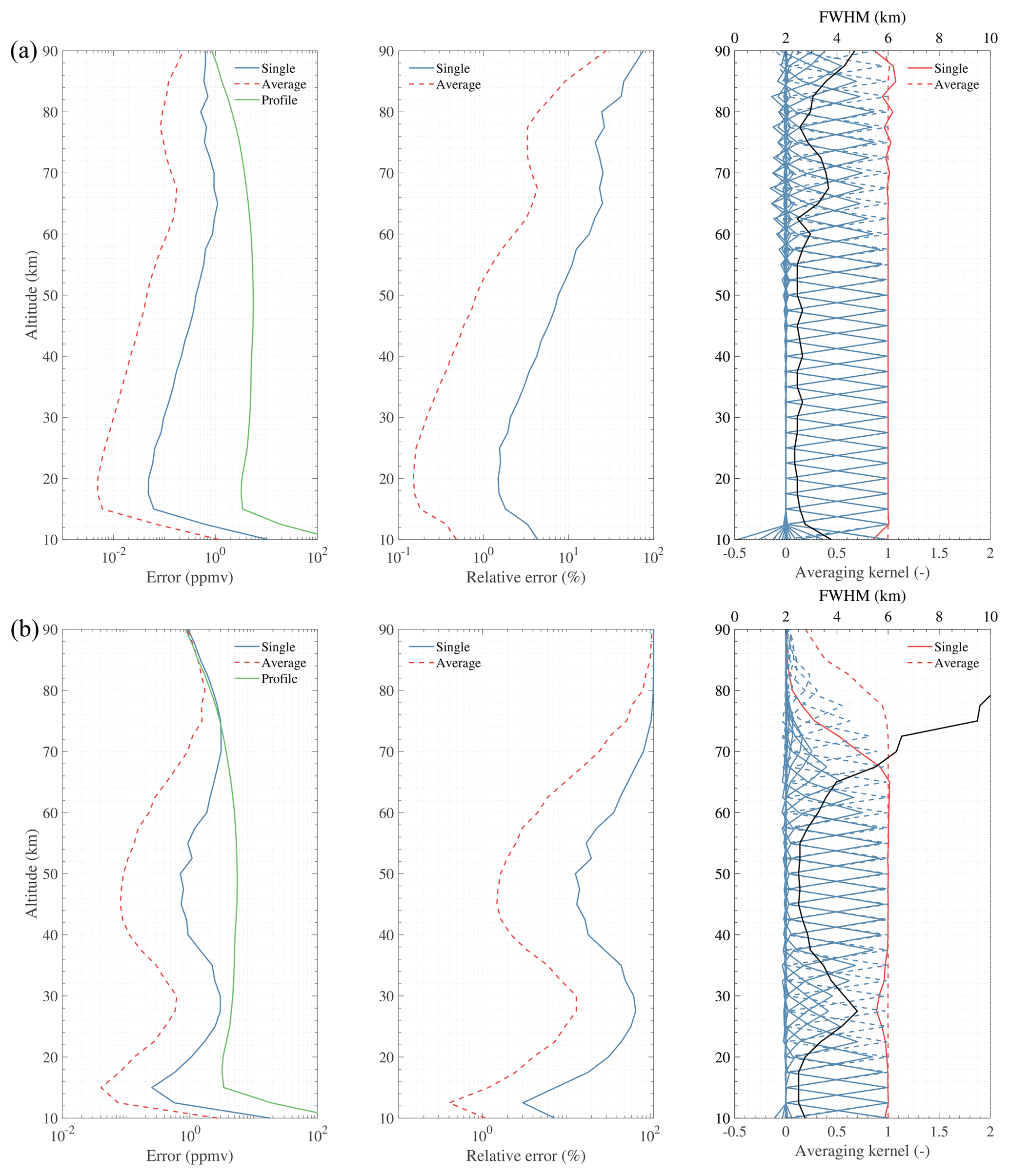
Figure 13 Simulation results of H₂O retrieval using 183.31 (a) and 657.9 GHz (b) lines. “Single” and “Average” represent the retrieval error using different noise. “Profile” represents the typical profile used in the simulation. The black solid line in the last panel represents the FWHM (i.e. vertical resolution).

4.3.1 Better precision products

Temperature, H₂O, O₃, HNO₃, HCl, N₂O, and ClO are treated as better precision products because of the good precision for a single scan measurement. These products can be used in scientific research directly.

Atmospheric temperature is the most important parameter that can be retrieved with a high signal-to-noise ratio at lower frequency or a good vertical resolution at high frequency by using O₂ lines. TALIS will use the 118 GHz radiometer to detect the atmospheric temperature profile, with the 240 and 643 GHz radiometers working as supplemental products. Results are shown in Fig. 12, and the sensitivity is significantly high at the 118 GHz band. Single scan precision is good from 15 to 60 km, with precision <2 K. The retrieval vertical resolution is 2.5–4 km below 50 km and 4–6 km from 50 to 80 km. The precision of the averaged measurement will be <1 K from 15 to 85 km.

“Wide” filters of MLS make measurements extending down into the troposphere where TALIS lacks sensitivity. However, the 240 GHz product can compensate for the loss of information since the precision is better in the upper troposphere (error <1 K for a vertical resolution of 2.5–3 km between 10 and 15 km). The result of the 643 GHz band is similar to that of the 240 GHz band.

Once the temperature profile is retrieved, the pressure profile can be calculated from the hydrostatic equilibrium equation using a known pressure and temperature at a reference tangent point. The pressure profile is not a direct product and is not shown here.

The H₂O profile, another key parameter, can be measured by 190 and 643 GHz radiometers. The 183.31 GHz line is generally used by humidity sounders to detect water vapour with good precision. Figure 13 shows the retrieval precision will be <10 % from 10 to 55 km by 190 GHz single scan measurement with a vertical resolution of 2.5–4 km. Averaged measurement has retrieval precisions <1 % at 10–55 km and <5 % at 10–80 km. The profile can also be retrieved by the 643 GHz radiometer with poorer precision.

O₃ has quite strong intensity in most spectral regions of TALIS. All the radiometers except 118 GHz can be used to observe this gas, which is important for energy balance (Fig. 14). The 240 GHz radiometer which covers the 235.7 GHz line has the highest O₃ sensitivity. The profile can be retrieved with a single scan precision <10 % from 10 to 55 km and the vertical resolution is 2.5–3 km. The vertical resolution will degrade to 3–6 km for altitudes higher than 70 km. By averaging the measurements, the precision will be <5 % at 10–70 km. The other two bands show good performance from 15 to 55 km with a single scan precision <10 %.

Figure 14 Simulation results of O₃ retrieval using 190 (a), 235.7 (b), and 657.5 GHz (c) lines. “Single” and “Average” represent the retrieval error using different noise. “Profile” represents the typical profile used in the simulation. The black solid line in the last panel represents the FWHM (i.e. vertical resolution).

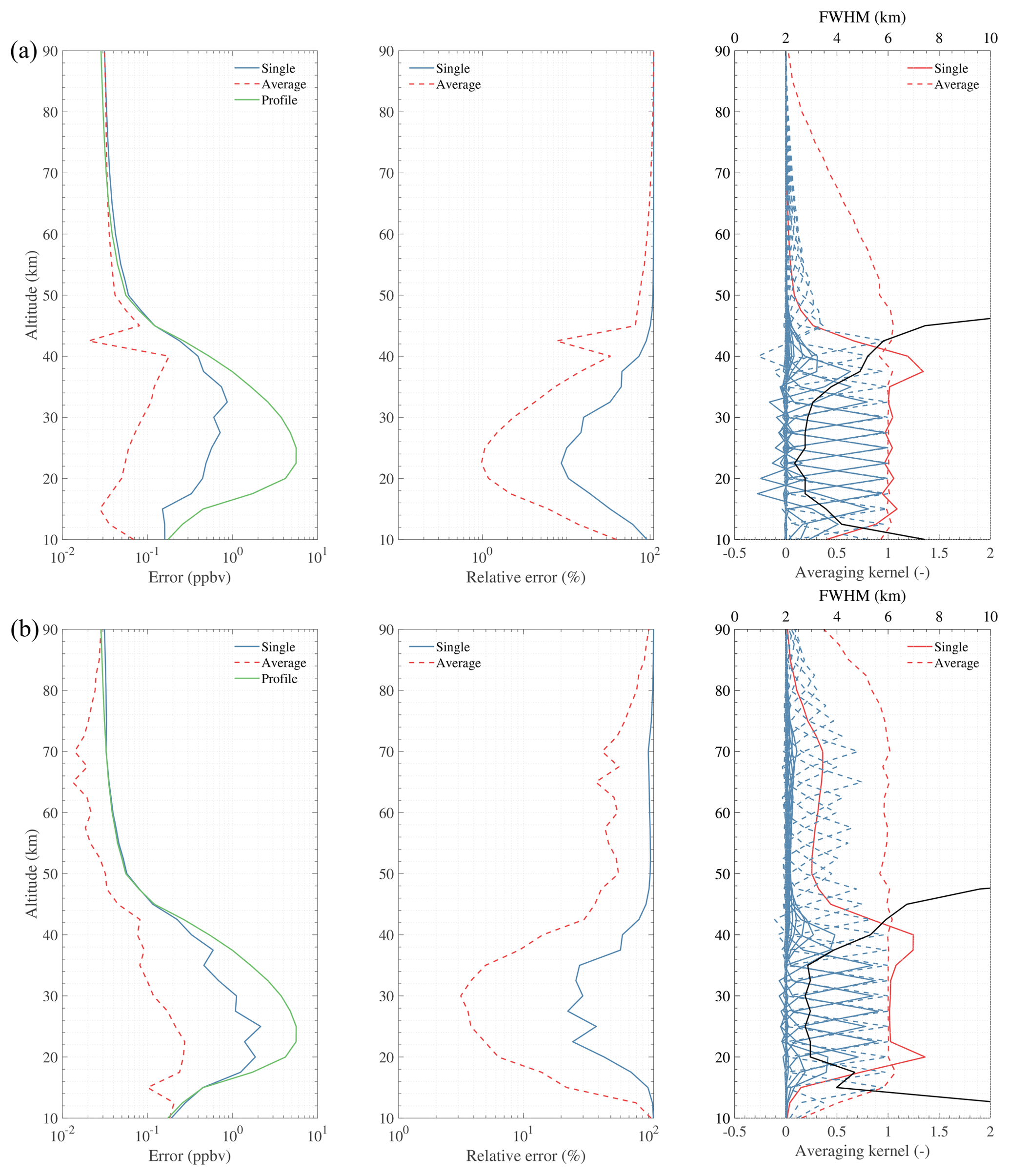
Figure 15 Simulation results of HNO₃ retrieval using 244 (a) and 656 GHz (b) lines. “Single” and “Average” represent the retrieval error using different noise. “Profile” represents the typical profile used in the simulation. The black solid line in the last panel represents the FWHM (i.e. vertical resolution).

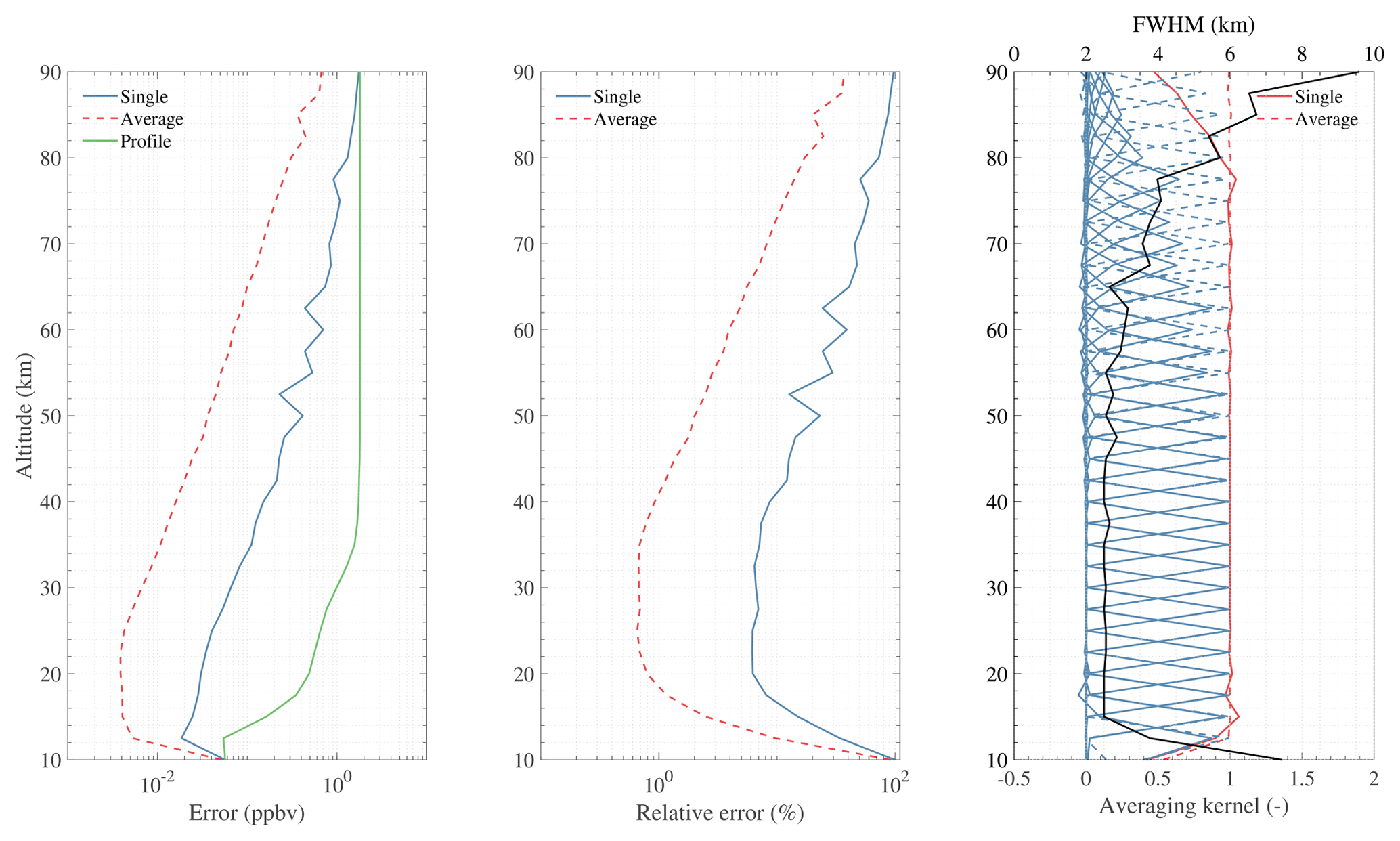
Figure 16 Simulation result of HCl retrieval using 624.9 GHz lines. “Single” and “Average” represent the retrieval error using different noise. “Profile” represents the typical profile used in the simulation. The black solid line in the last panel represents the FWHM (i.e. vertical resolution).

HNO₃ is a common species in the stratosphere and has relatively strong lines at 240 and 643 GHz bands. Figure 15 shows the results of HNO₃ retrievals. The 240 GHz radiometer can measure HNO₃ at a 15–32 km altitude range with a single scan precision <30 % and the vertical resolution is 2.5–3 km. Averaging the measurements can improve the retrieval with a precision <10 % from 15 to 35 km. The 643 GHz signal is stronger than that in the 240 GHz band, but it is strongly absorbed by O₃ below about 30 km. However, after averaging the measurements, information can be retrieved between 15 and 70 km with a precision better than 60 %.

Figure 16 shows the expected precision of HCl observation. HCl can be measured at 15–50 km with <20 % single scan relative error with the vertical resolution of 2.5–3 km. By averaging the measurements, the precision will be <10 % at 12–72 km.

N₂O can be retrieved from the band at 190 GHz in the upper troposphere, while the band at 643 GHz can provide more information and good precision in the stratosphere. Figure 17 shows that the single scan precision of 643 GHz is <20 % at 12–32 km with the vertical resolution of 2.5 km. By averaging the measurements, the precision will be <10 % from 10 to 42 km. The 190 GHz can give a similar precision at 10–20 km.

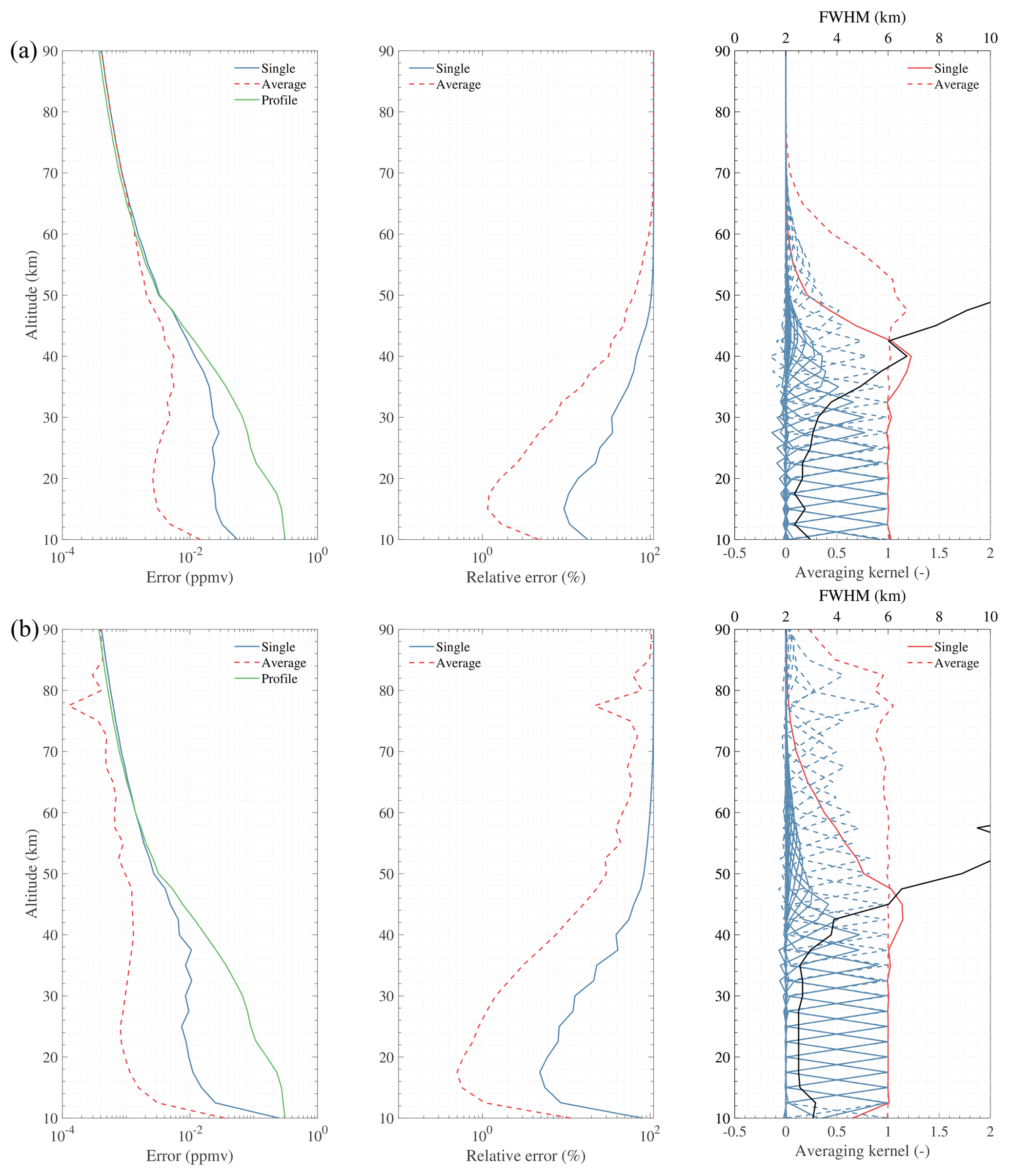
Figure 17 Simulation results of N₂O retrieval using 200.98 (a) and 652.834 GHz (b) lines. “Single” and “Average” represent the retrieval error using different noise. “Profile” represents the typical profile used in the simulation. The black solid line in the last panel represents the FWHM (i.e. vertical resolution).

ClO can be retrieved from radiances measured by the 190 and 643 GHz bands (Fig. 18). However, the result shows that the best retrievals are performed from the band at 643 GHz, but information can also be retrieved from the 190 GHz radiometer with poorer precision. Single scan measurement from the 643 GHz radiometer can be used to obtain ClO with <40 % precision from 30 to 45 km, and the vertical resolution is about 2.5–4 km throughout the useful range. By averaging the measurements, precision will be <30 % from 23 to 57 km. Since ClO vanishes in the middle stratosphere (30–40 km) during nighttime, the precision will be relatively worse in the nighttime. In the polar regions, the relative precision will be better between 20 and 25 km during chlorine activation.

Figure 18 Simulation results of ClO retrieval using 203.4 (a) and 649.45 GHz (b) lines. “Single” and “Average” represent the retrieval error using different noise. “Profile” represents the typical profile used in the simulation. The black solid line in the last panel represents the FWHM (i.e. vertical resolution).

4.3.2 Medium precision products

Medium precision products including CO, HCN, and CH₃Cl mean that their single scan retrieval precisions are not satisfying but can be used to some degree. There is a choice for the user to select the single scan or averaged products.

CO can be measured using the 230.538 and 661.07 GHz lines. Figure 19 shows that the 240 GHz radiometer can provide CO information with 30 %–90 % single scan precision from 10 to 90 km. The vertical resolution is in the range 3.5–5.5 km from the upper troposphere to the lower mesosphere, degrading to 6–10 km in the upper mesosphere. By using averaged measurements, CO can be retrieved with <30 % relative error at the range of 10–90 km. However, the retrieval of the 643 GHz measurement shows poorer precision.

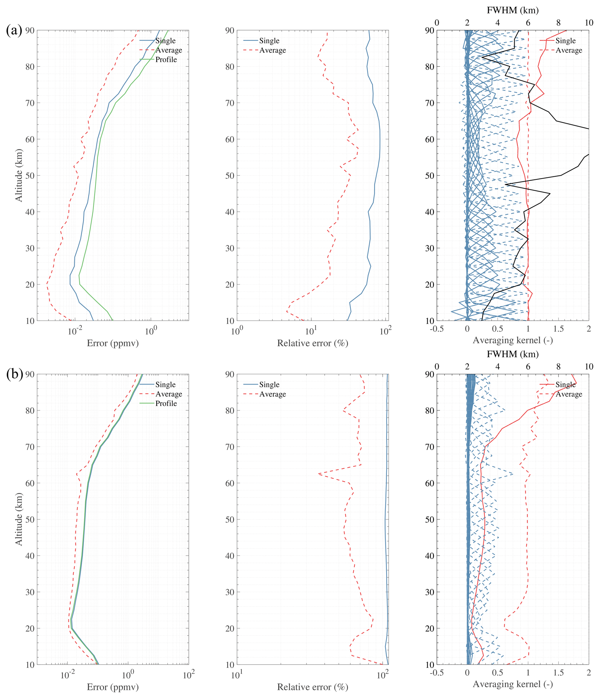
Figure 19 Simulation results of CO retrieval using 230.538 (a) and 661.07 GHz (b) lines. “Single” and “Average” represent the retrieval error using different noise. “Profile” represents the typical profile used in the simulation. The black solid line in the last panel represents the FWHM (i.e. vertical resolution).

HCN is measured by the 190 GHz radiometer at the 177.26 GHz line. The single scan precision is <50 % from 12 to 28 km and the vertical resolution is about 5 km at the height of 30 km, degrading to 8 km at about 40 km (Fig. 20). By averaging the measurements, the relative error will be <30 % at 10–40 km.

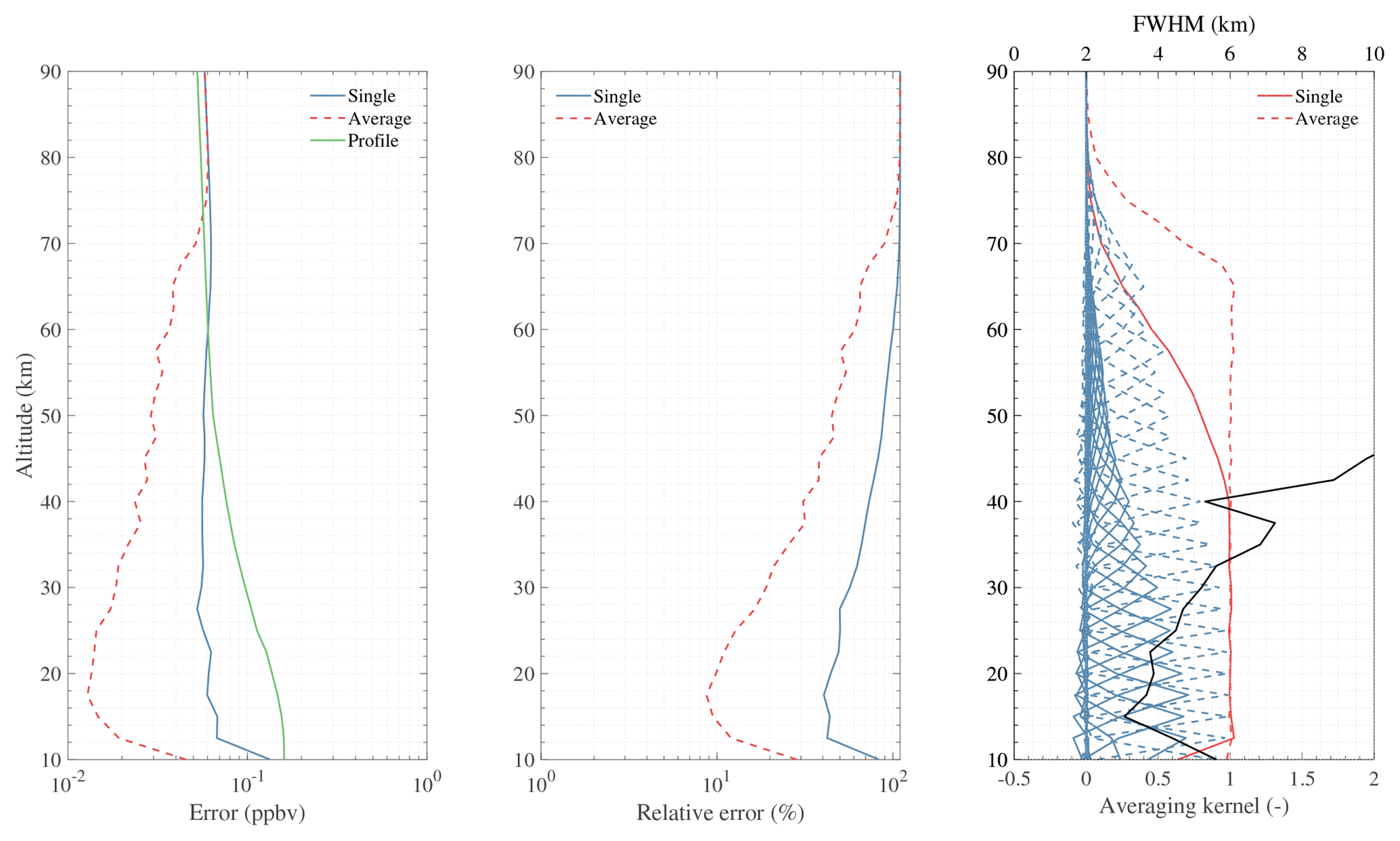
Figure 20 Simulation result of HCN retrieval using 177.26 GHz lines. “Single” and “Average” represent the retrieval error using different noise. “Profile” represents the typical profile used in the simulation. The black solid line in the last panel represents the FWHM (i.e. vertical resolution).

CH₃Cl can be measured by the 643 GHz radiometer. As the result shows (Fig. 21), the 649.5 GHz band is suitable for CH₃Cl observation in the upper troposphere and lower stratosphere. It can be measured with <30 % single scan precision from 12 to 23 km, with <20 % averaged precision from 10 to 30 km. The vertical resolution is about 3–4 km over most of the useful range.

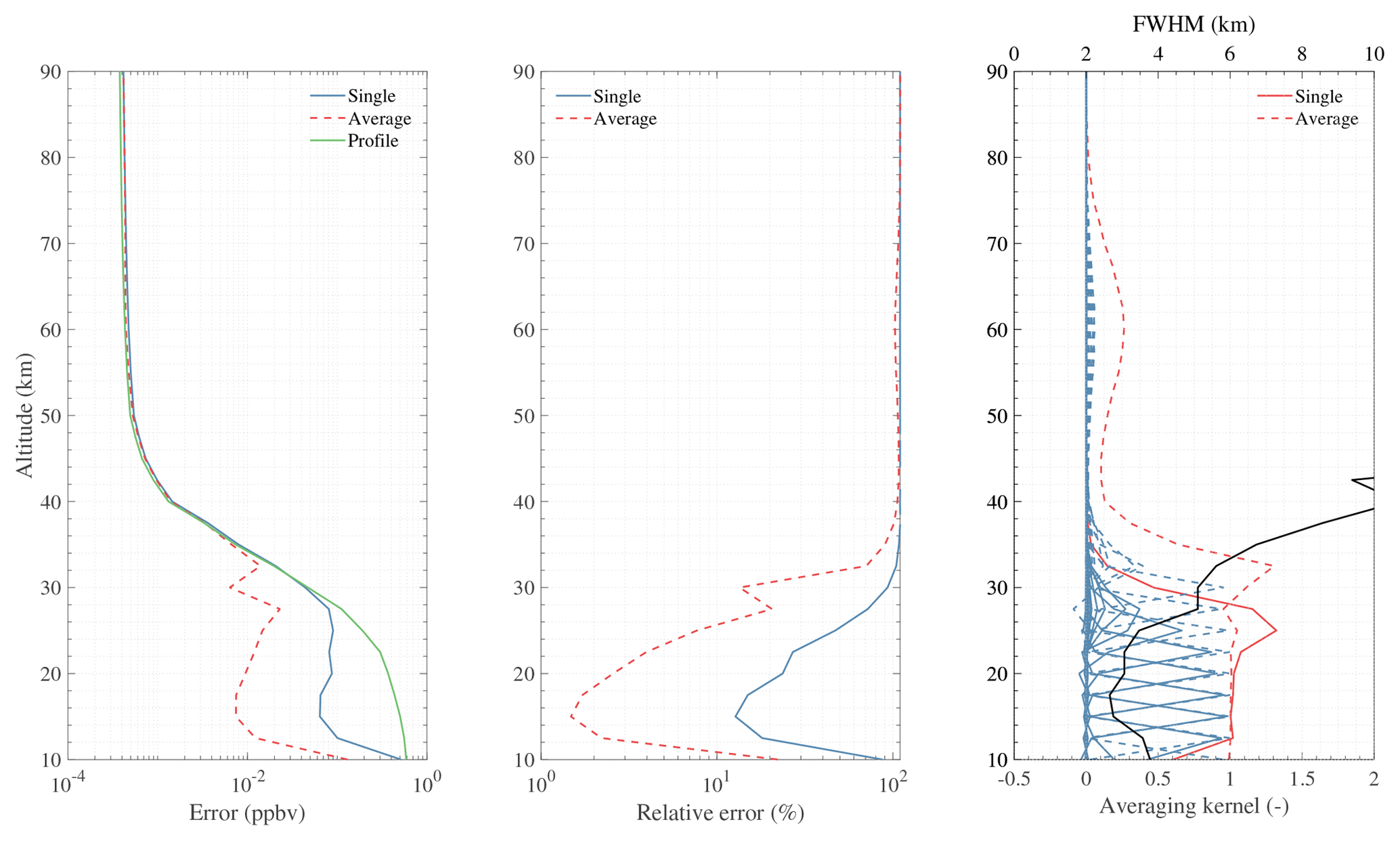
Figure 21 Simulation results of CH₃Cl retrieval using 649.5 GHz lines. “Single” and “Average” represent the retrieval error using different noise. “Profile” represents the typical profile used in the simulation. The black solid line in the last panel represents the FWHM (i.e. vertical resolution).

4.3.3 Poor precision products

There are several weak lines in the spectral regions of TALIS, such as HOCl, BrO, and HO₂. Significant averaging must be done to these measurements in order to obtain reliable and satisfying precision.

The 635.87 GHz line is the most appropriate line for HOCl observation. However, the single scan retrieval has a poor precision of 60 %–80 % at 25–45 km with the vertical resolution of about 4–6 km. Figure 22 reveals that HOCl can be retrieved from 20 to 50 km with an averaged measurement precision of <50 %.

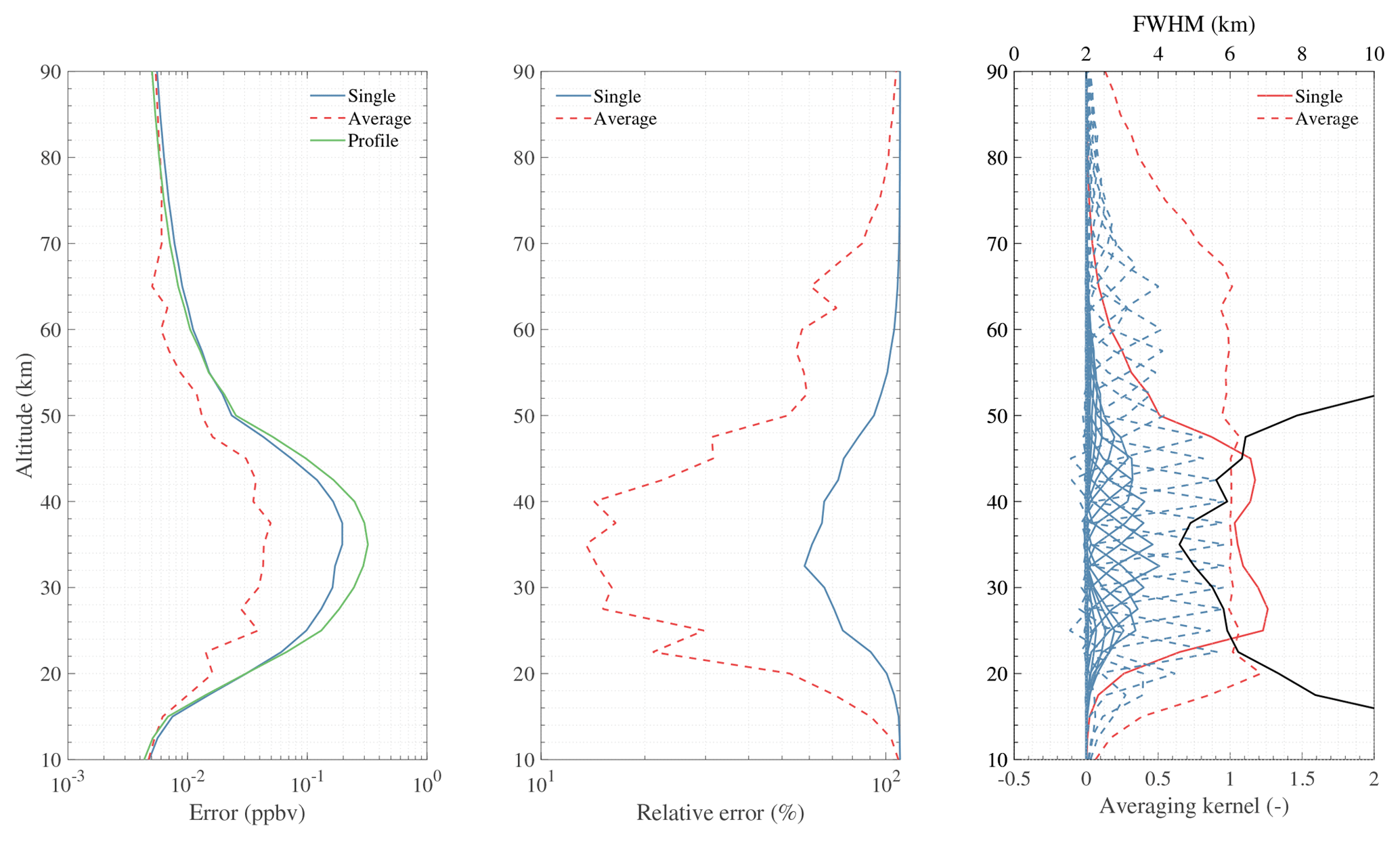
Figure 22 Simulation result of HOCl retrieval using 635.87 GHz lines. “Single” and “Average” represent the retrieval error using different noise. “Profile” represents the typical profile used in the simulation. The black solid line in the last panel represents the FWHM (i.e. vertical resolution).

BrO can be measured by using the 624.768 GHz spectral line. Figure 23 shows the simulation result of BrO retrieval. As the averaging kernel reveals, there is almost no useful information in single scan measurement because of the quite poor signal-to-noise ratio. Therefore, averaging is needed to obtain reliable and scientific results. The error is 50 % from 24 to 48 km with the vertical resolution of about 4 km.

Figure 23 Simulation results of BrO retrieval using 624.768 GHz lines. “Single” and “Average” represent the retrieval error using different noise. “Profile” represents the typical profile used in the simulation. The black solid line in the last panel represents the FWHM (i.e. vertical resolution).

HO₂ can be measured by the 643 GHz radiometer with <50 % precision at the vertical range of 30–90 km by using averaged data (Fig. 24). The precision of single scan retrieval is 55 %–70 % at 40–75 km, which is not desirable because of the weak signal. The vertical resolution is about 6 km.

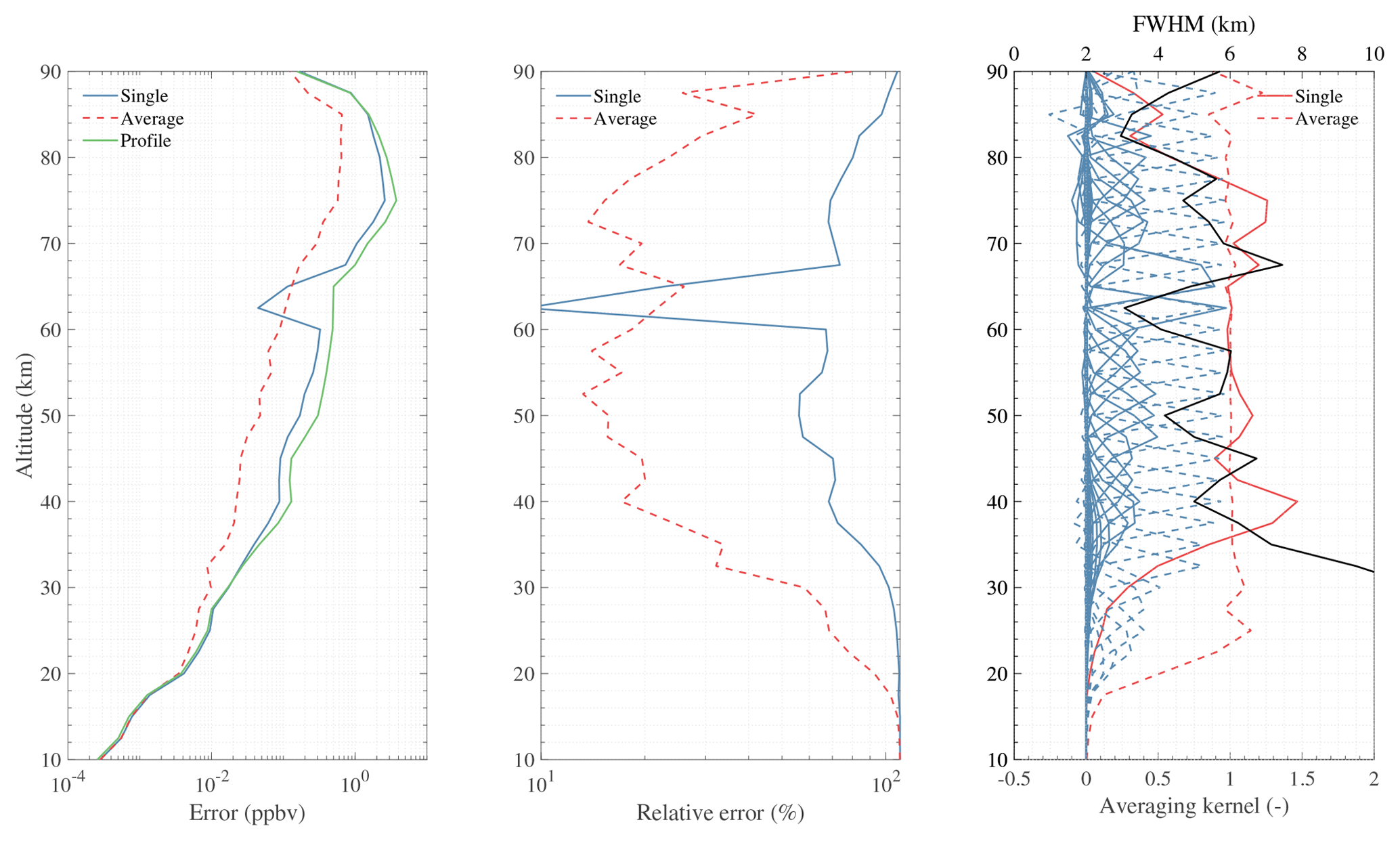
Figure 24 Simulation results of HO₂ retrieval using 649.701 GHz lines. “Single” and “Average” represent the retrieval error using different noise. “Profile” represents the typical profile used in the simulation. The black solid line in the last panel represents the FWHM (i.e. vertical resolution).

4.3.4 Promising products

The unique products are the target species which are not covered by the Aura MLS but which are covered by TALIS. There are four gases: NO, NO₂, H₂CO, and SO₂ (normal VMR). However, their signals all have weak intensity and must be averaged to improve the retrieval precision.

NO (daytime) can be retrieved from averaged data with <50 % precision at 28–90 km (Fig. 25), while it vanishes in the nighttime. The vertical resolution is about 4–10 km, while its single scan measurement has little information in the area where NO largely exists.

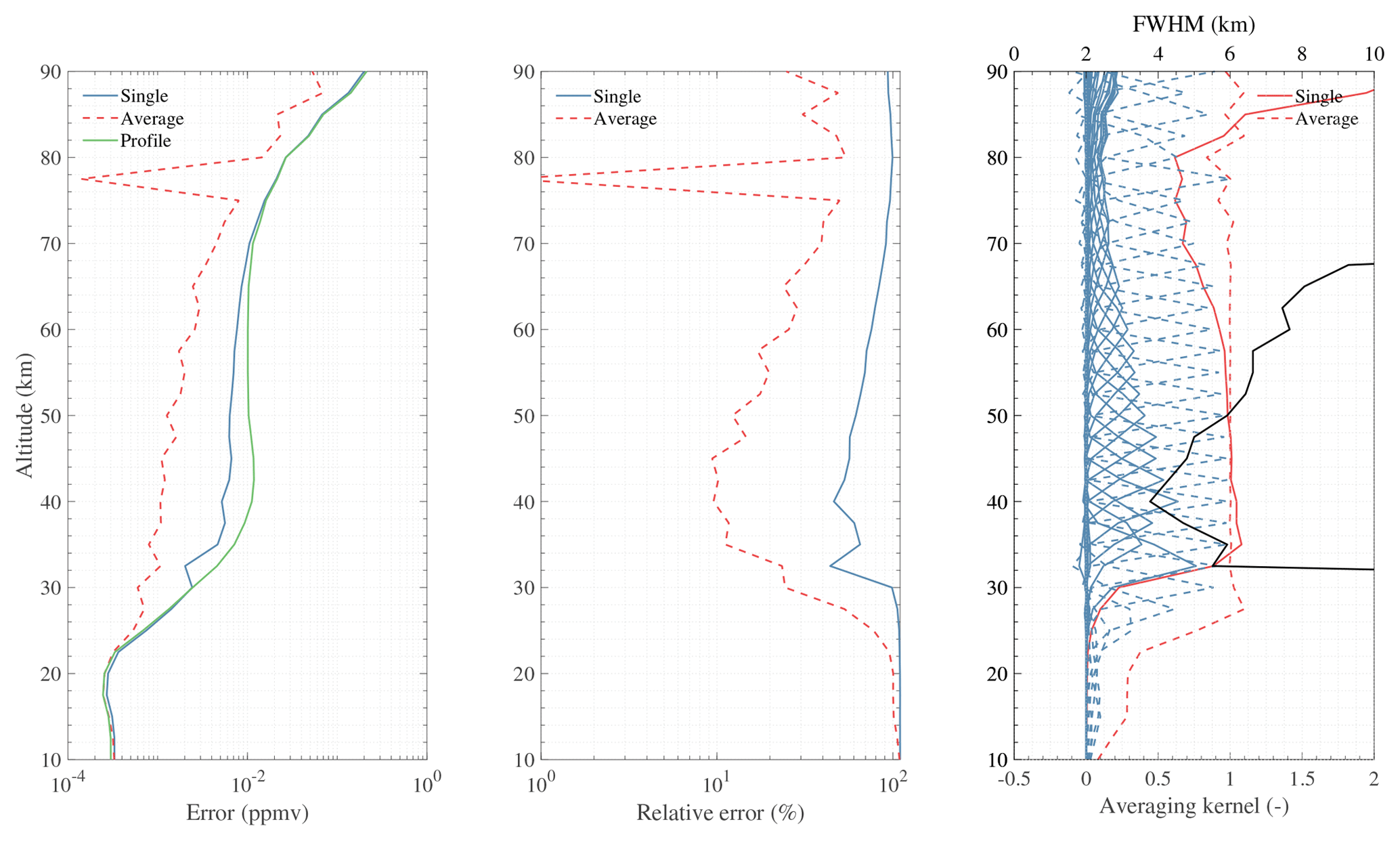
Figure 25 Simulation result of NO retrieval using 651.75 GHz lines. “Single” and “Average” represent the retrieval error using different noise. “Profile” represents the typical profile used in the simulation. The black solid line in the last panel represents the FWHM (i.e. vertical resolution).

NO₂ (nighttime) has a weak line in the spectrum of the 240 GHz band, and it vanishes in the daytime. Figure 26 shows that only averaged measurement can provide some information at 20–40 km, with a precision of about 40 %–60 % in the nighttime. The vertical resolution is about 5 km.

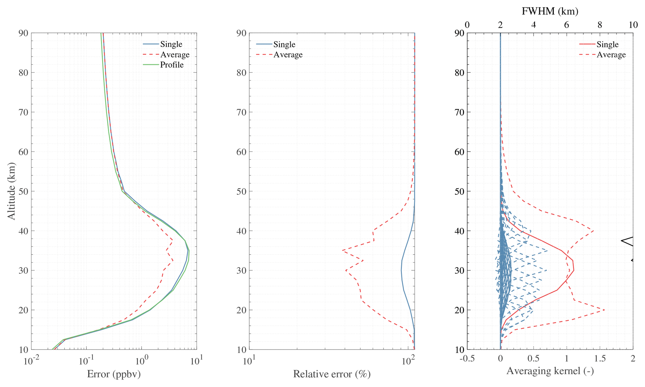
Figure 26 Simulation result of NO₂ retrieval using 232.7 GHz lines. “Single” and “Average” represent the retrieval error using different noise. “Profile” represents the typical profile used in the simulation. The black solid line in the last panel represents the FWHM (i.e. vertical resolution).

Although H₂CO has a line at 656.45 GHz, its emission radiance is too weak. Almost no useful information can be obtained (Fig. 27). However, this line has the potential to measure H₂CO. More average or other effective methods should be applied to get acceptable precision.

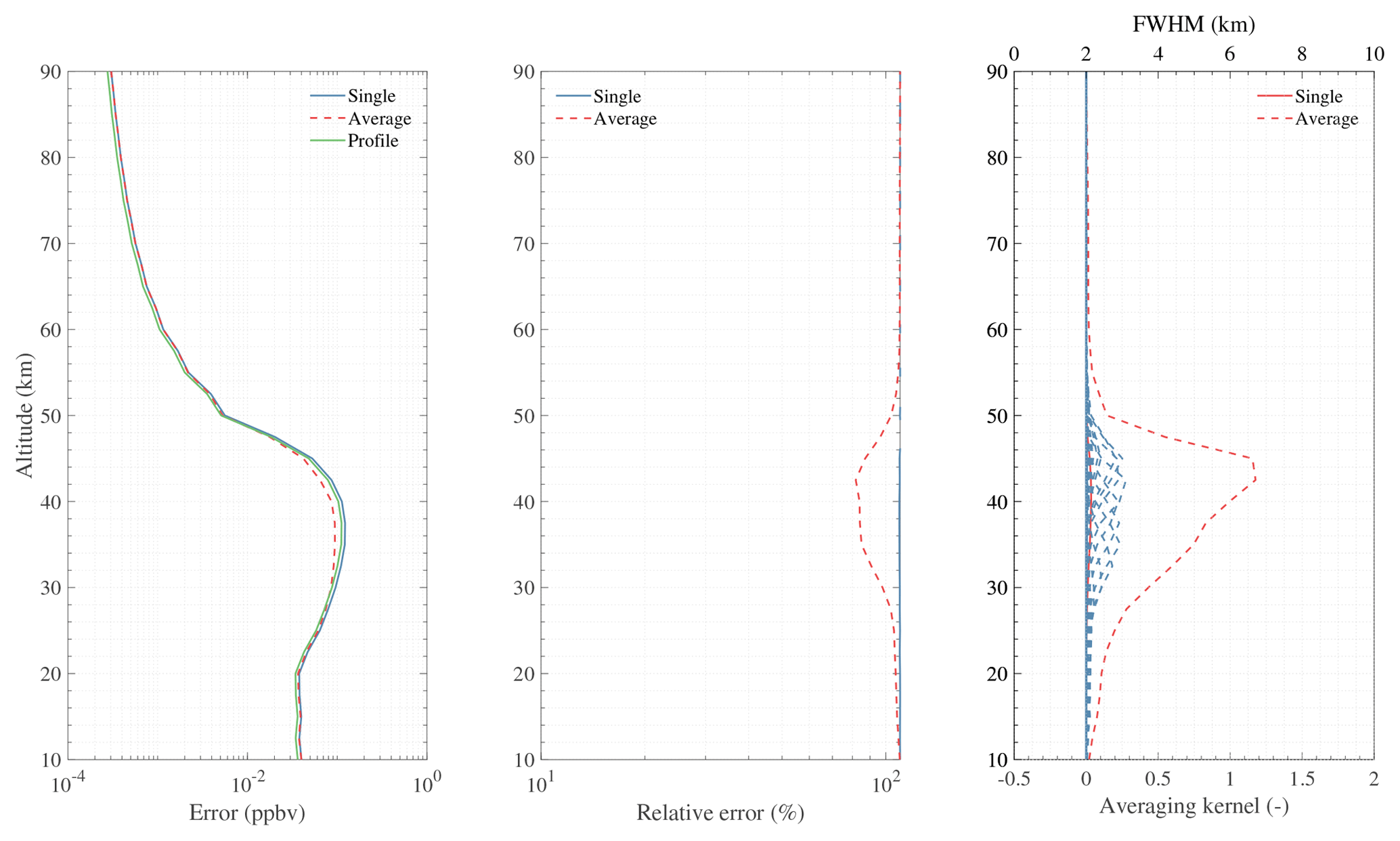
Figure 27 Simulation result of H₂CO retrieval using 656.45 GHz lines. “Single” and “Average” represent the retrieval error using different noise. “Profile” represents the typical profile used in the simulation. The black solid line in the last panel represents the FWHM (i.e. vertical resolution).

The MLS standard SO₂ product is taken from the 240 GHz retrieval, but is only effective when its concentration is significantly enhanced. TALIS has both 240 and 643 GHz radiometers, which cover the lines of SO₂. The 240 GHz radiometer can be used to measure SO₂ in the same way as MLS. The 643 GHz radiometer can give the concentration of the nominal background. The averaged result shows that SO₂ can be retrieved at 14–20 km, 46–70 km with the relative error about <50 % (Fig. 28). The vertical resolution is about 6 km.

Figure 28 Simulation result of SO₂ retrieval using 659 GHz lines. “Single” and “Average” represent the retrieval error using different noise. “Profile” represents the typical profile used in the simulation. The black solid line in the last panel represents the FWHM (i.e. vertical resolution).

5 Conclusions

Simulation analysis for temperature and chemical species retrieval has been performed to assess the measurement performance of TALIS and to support the mission. This study mainly focuses on a large number of important chemical species in the middle and upper atmosphere which can be observed by the limb sounder. The results are summarised in Table 3.

Table 3 Simulation results of TALIS retrieval precision.

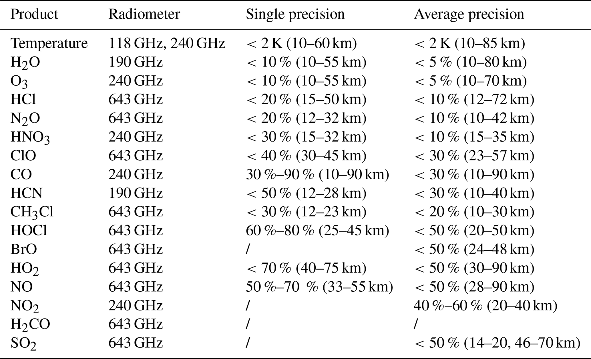
Seven species show high sensitivity, sufficient for scientifically useful single profile retrievals; 118, 240, and 643 GHz observations of O₂ are used to estimate the temperature profile, which is quite important in meteorology. The 118 GHz radiometer can obtain temperature with a precision <2 K at 10–60 km and the 240 and 643 GHz radiometers can provide more information in the upper troposphere (precision <1 K at 10–15 km). The 190 GHz radiometer can be used to measure H₂O with a precision <10 % at 10–55 km and give information of upper tropospheric humidity. O₃ can be measured by three radiometers, and the 240 GHz radiometer has the best precision. The precision is <10 % from 10 to 55 km by single scan measurement. HNO₃ can be derived from 240 GHz retrieval with a precision <30 % at 15–32 km. The precision of HCl single scan retrieval is <20 % over most of the useful range. The 643 GHz radiometer can give a good estimate of the N₂O profile, with a precision <20 % at 12–32 km. The single scan precision of ClO measured by the 643 GHz radiometer is about <40 % in the area where ClO mainly exists. CH₃Cl can be measured in the upper troposphere and low stratosphere with a precision of about 30 %. The profile of CO retrieved from 240 GHz measurement is better than that from 643 GHz measurement. The best sensitivity is found between 70 and 90 km where the VMR of CO is large, and the precision is about 50 %. HCN has 50 % single scan precision at 12–28 km, which may need to be averaged. Other measurements, such as HO₂, HOCl, NO, NO₂, BrO, SO₂, and H₂CO, must be significantly averaged before scientific use because of the weak signals.

Apart from these products, some potential products will be discussed in the future works. Line-of-sight wind is important information which could be measured by TALIS. Cloud ice water content (IWC) is also an essential product provided by the passive microwave radiometer. Future studies will also investigate the Zeeman effect since it polarises and changes the shape of the O₂ lines.

TALIS has the potential to monitor chemical composition in the whole of Earth's atmosphere, which is important for numerical weather prediction models and to characterise the long-time change in climate. Measurement data can be used for atmospheric chemistry and dynamics study, which is quite important for geoscience. This paper is the preliminary analysis of the instrument. More studies such as calibration research and error analysis will be performed in the future.