Towards objective identification and tracking of convective outflow boundaries in next-generation geostationary satellite imagery

Sudden wind direction and speed shifts from outflow boundaries (OFBs) associated with deep convection significantly affect weather in the lower troposphere. Specific OFB impacts include rapid variation in wildfire spread rate and direction, the formation of convection, aviation hazards, and degradation of visibility and air quality due to mineral dust aerosol lofting. Despite their recognized importance to operational weather forecasters, OFB characterization (location, timing, intensity, etc.) in numerical models remains challenging. Thus, there remains a need for objective OFB identification algorithms to assist decision support services. With two operational next-generation geostationary satellites now providing coverage over North America, high-temporal- and high-spatial-resolution satellite imagery provides a unique resource for OFB identification. A system is conceptualized here designed around the new capabilities to objectively derive dense mesoscale motion flow fields in the Geostationary Operational Environmental Satellite 16 (GOES-16) imagery via optical flow. OFBs are identified here by isolating linear features in satellite imagery and backtracking them using optical flow to determine if they originated from a deep convection source. This “objective OFB identification” is tested with a case study of an OFB-triggered dust storm over southern Arizona. The results highlight the importance of motion discontinuity preservation, revealing that standard optical flow algorithms used with previous studies underestimate wind speeds when background pixels are included in the computation with cloud targets. The primary source of false alarms is the incorrect identification of line-like features in the initial satellite imagery. Future improvements to this process are described to ultimately provide a fully automated OFB identification algorithm.

1 Introduction

Downburst outflows from associated deep convection (Byers and Braham Jr., 1949; Mitchell and Hovermale, 1977) play a significant, dynamic role in modulation of the lower troposphere. Their direct impacts to society are readily apparent – capsizing boats on lakes and rivers with winds that seem to “come out of nowhere” (e.g., the Branson, MO, duck boat accident; Associated Press, 2018), causing shifts in wildfire motion and fire intensity that put firefighters in harm's way (e.g., the Waldo Canyon and Yarnell Hill fires; Hardy and Comfort, 2015; Johnson et al., 2014) and threatening aviation safety at regional airports with sudden shifts from head to tail winds and turbulent wakes (Klingle et al., 1987; Uyeda and Zrnić, 1986). In the desert southwest, convective outflows can loft immense amounts of dust, significantly reducing surface visibility and air quality for those within the impacted area (e.g., Idso et al., 1972; Raman et al. 2014). These outflows are commonly associated with rapid temperature, pressure, and moisture changes at the surface (Mahoney, 1988). Furthermore, the collision of outflows from adjacent storms can serve as the focal point of incipient convection or the intensification of nascent storms (Mueller et al., 2003; Rotunno et al., 1988).

Despite the understood importance of deep convection and convectively driven outflows, high-resolution models struggle to characterize and identify them (e.g., Yin et al., 2005). At present, outflow boundaries (OFBs) are instead most effectively monitored in real time at operational centers around the world with surface, radar, and satellite data. Satellites often offer the only form of observation in remote locations. The most common method for detecting outflows via satellite data involves the identification of clouds formed by strong convergence at the OFB leading edge. When the lower troposphere is dry, OFBs may be demarcated by an airborne “dust front”, after passing over certain surfaces prone to deflation by frictional winds (Miller et al., 2008). The task of identifying OFBs can prove quite challenging and would benefit greatly from an objective means of feature identification and tracking for better decision support services.

The Advanced Baseline Imager (ABI), an imaging radiometer carried onboard the Geostationary Operational Environmental Satellite R (GOES-R) era systems, offers a leap forward in capabilities for the real-time monitoring and characterization of OFBs. Its markedly improved spatial (0.5 vs. 1.0 km visible, 2 km vs. 4 km infrared), spectral (16 vs. 5 spectral bands), and temporal (5 min vs. 30 min continental US, and 10 min vs. 3 h full disk) resolution provides new opportunities for passive sampling of the atmosphere over the previous generation (Schmit et al., 2017). The vast improvement of temporal resolution alone (which includes mesoscale sectors that refresh as high as 30 s) allows for dramatically improved tracking of convection (Cintineo et al., 2014; Mecikalski et al., 2016; Sieglaff et al., 2013), fires and pyroconvection (Peterson et al., 2015, 2017, 2018), ice flows, and synoptic-scale patterns (Line et al., 2016). This higher temporal resolution makes the identification of features like OFBs easier as well because of greater frame-to-frame consistency.

The goal of this work is to use ABI information towards the objective identification of OFBs. One of the notable challenges in the satellite identification of OFBs over radar or models is the lack of auxiliary information. When working with a radar or a numerical model framework, for example, additional information is available on the flow, temperature, and pressure tendency of the boundary. Without that information, however, forecasters must rely on their knowledge of gust front dynamics to identify OFBs in satellite imagery. Here, we introduce the concept of objectively derived motion using GOES-16 ABI imagery for feature identification via an advanced optical flow method, customized to the problem at hand. A case study of a convectively triggered OFB and accompanying haboob dust front is presented in 5 min GOES-16 contiguous United States (CONUS) sector information, as a way of evaluating and illustrating the potential of the framework.

This paper is outlined as follows. The background for objective motion extraction and OFB identification is presented in Sect. 2. The optical flow methods developed for this purpose are discussed in Sect. 3. Section 4 presents the case study test of the current algorithm, and Sect. 5 concludes the paper with a discussion on plans for future work in objective feature identification from next-generation geostationary imagers of similar fidelity as the GOES-R ABI, which are presently coming online around the globe.

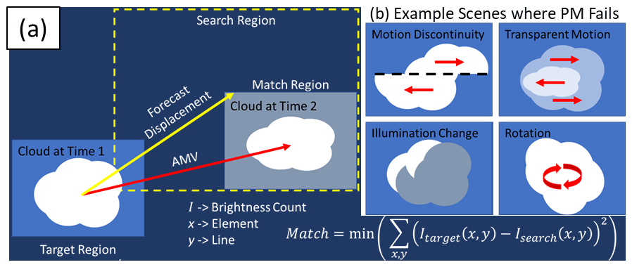
Figure 1 Schematic of (a) the PM optical flow scheme used by AMVs (e.g., Bresky et al., 2012), which finds a suitable target to track (e.g., the cloud at time 1), forecasts the displacement with numerical models (yellow arrow and dashed box), and iteratively searches for the target at time 2 by minimizing the sum of square error to get the AMV (red arrow). (b) Example cloud evolution types mentioned in the text for which the approach shown in (a) fails.

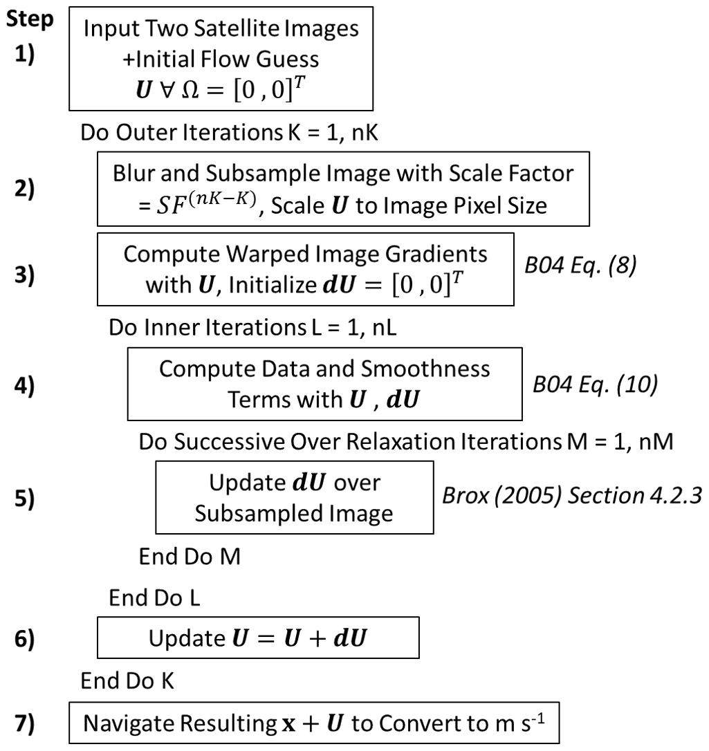
Figure 2 Flowchart of the B04 optical flow approach used here. Note that SF, nK, nL, and nM are defined in Table 1.

2 Background

2.1 Previous work in OFB detection

The objective identification of OFBs in meteorological data has been a topic of scientific inquiry for more than 30 years. Uyeda and Zrnić (1986) and Hermes et al. (1993) use detections of wind shifts in terminal Doppler radar velocity measurements to isolate regions of strong radial shear associated with OFBs. Smalley et al. (2007) include the “fine line” reflectivity structure of biological- and precipitation-sized particles to identify OFBs via image template matching. Chipilski et al. (2018) considered the OFB objective identification in numerical models using similar image processing techniques, but with additional dynamical constraints on vertical velocity magnitudes and mean sea level pressure tendency. Objective OFB identification has not been demonstrated to date with the new ABI observations of the GOES-R satellite series. Identification via satellite imagery would be valuable for local deep convection nowcasting algorithms, which use boundary presence as a predictor field (Mueller et al., 2003; Roberts et al., 2012), and for operational centers around the world that may not have access to ground-based Doppler radar data.

Traditionally, forecasters have identified OFBs in satellite imagery by visually identifying the quasi-linear low-level cloud features and backtracking them to an associated deep convection source. Previous objective motion derivation algorithms are not designed to yield the dense wind fields, in which motion is estimated at every image pixel, necessary for identifying and tracking features such as OFBs (Bedka et al., 2009; Velden et al., 2005). In fact, the original image window-matching atmospheric motion vector (AMV) algorithms produce winds only over targets deemed acceptable for tracking by preprocessing checks on the number of cloud layers in a scene, brightness gradient strength, and patch coherency. The targets are further filtered with post-processing checks on acceleration and curvature through three-frame motion and deviation from numerical model flow (Bresky et al., 2012; Nieman et al., 1997; Velden et al., 1997; More in Sect. 2.2). These practices were followed for a very practical reason – AMV algorithms were tailored for model data assimilation. In the formation of the model analysis, observational data must be heavily quality-controlled, with outliers removed, to minimize data rejection. Here, information such as OFBs would be rejected due to the detailed space–time structure of actual convection, which is typically poorly represented by the numerical model.

Deriving two-dimensional flow information at every point in the imagery would require either modification of previous AMV schemes or post-processing of the AMV data via objective analysis (e.g., Apke et al., 2018). The latter typically will not capture motion field discontinuities, resulting in incorrect flows near feature edges (Apke et al., 2016). To capture such discontinuities in a dense flow algorithm, new computer vision techniques, such as the gradient-based methods of optical flow, must be adopted.

2.2 Optical flow techniques

Optical flow gradient-based techniques derive motion within fixed windows, thus eliminating the reliance on models for defining a search region. A core assumption of many optical flow techniques is brightness constancy (Horn and Schunck, 1981). Considering two image frames, brightness constancy states that the image intensity I at some point $\mathit{x}={\left[x,y\right]}^T$ is equal to the image intensity in the subsequent frame at a new point, x+U, where, with a translation model, $\mathbf{U}={\left[u,v\right]}^T$ represents the flow components of the image over the time interval (Δt) between the two images:

$$\begin{array}{}\text{(1)}& I\left(\mathit{x},t\right)=I(\mathit{x}+\mathbf{U},t+\mathrm{\Delta }t).\end{array}$$

Equation (1) can be linearized to solve for the individual flow components, u and v:

$$\begin{array}{}\text{(2)}& \mathrm{\nabla }I\cdot \mathbf{U}+I_{\mathrm{t}}=\mathrm{0}.\end{array}$$

where $\mathrm{\nabla }I=[I_x,I_y]$ represents the intensity gradients in the x and y direction, and I_t represents the temporal gradient of intensity. For one image pixel, Eq. (2) contains two unknowns with a simple translation model for U; therefore, it cannot be solved pointwise. One well-known approach to solving this so-called “aperture problem” is the Lucas–Kanade method, hereafter the LK method, which considers a measurement neighborhood of the intensity space and time gradients (e.g., Baker and Matthews, 2004; Bresky and Daniels, 2006). The use of neighborhoods, or image windows, to derive optical flow is called a local approach. Another seminal approach was introduced by Horn and Schunck (1981; the HS method), which solves the aperture problem by adding an additional smoothness constraint to the brightness constancy assumption and minimizing an energy magnitude between two images:

$$\begin{array}{}\text{(3)}& E\left(\mathbf{U}\right)=\int \underset{\mathrm{\Omega }}{\int }{\left(\mathrm{\nabla }I\cdot \mathbf{U}+I_{\mathrm{t}}\right)}^{\mathrm{2}}+\mathit{\alpha }(\mathrm{|}{\mathrm{\nabla }}_{\mathrm{2}}u{\mathrm{|}}^{\mathrm{2}}+\mathrm{|}{\mathrm{\nabla }}_{\mathrm{2}}v{\mathrm{|}}^{\mathrm{2}})d\mathit{x},\end{array}$$

where E(U) represents an energy functional to be minimized over all image pixels Ω, α is a constant weight used to control the smoothness of the flow components u(x) and v(x), and ${\mathrm{\nabla }}_{\mathrm{2}}=[\partial /\partial x,\partial /\partial y{]}^T$. This derivation is called a global approach, whereby the optical flow u(x)and v(x) at each pixel is found that minimizes the quantity of Eq. (3) by deriving the Euler–Lagrange equations and numerically solving the linear system of equations with Gauss–Seidel iterations.

Readers can contrast the HS method with the optical flow algorithm used in GOES AMVs, referred to as “patch matching” (PM; Fortun et al., 2015). In PM, a target (e.g., a 5×5 pixel box) identified as suitable for tracking is iteratively searched for in a sequential image within a reasonable search area (Fig. 1a). The motion is identified by which candidate target (e.g., another 5×5 pixel box displaced by the optical flow motion) in the sequential image best matches the initial target, typically by minimizing the sum of square error between the target and the candidate brightness values (Daniels et al., 2010; Nieman et al., 1997). The reader can draw similarities to the HS method by formulating the PM approach as an energy equation to be minimized:

$$\begin{array}{}\text{(4)}& E\left(\mathbf{U}\right)=\sum _{n\in T}{\left|I\left({\mathit{x}}_n,t\right)-I\left({\mathit{x}}_n+\mathbf{U},t+\mathrm{\Delta }t\right)\right|}^{\mathrm{2}},\end{array}$$

where the minimum in E is found by computing Eq. (4) at every candidate target in the search region. As E is only minimized within the target area T, PM represents a local method.

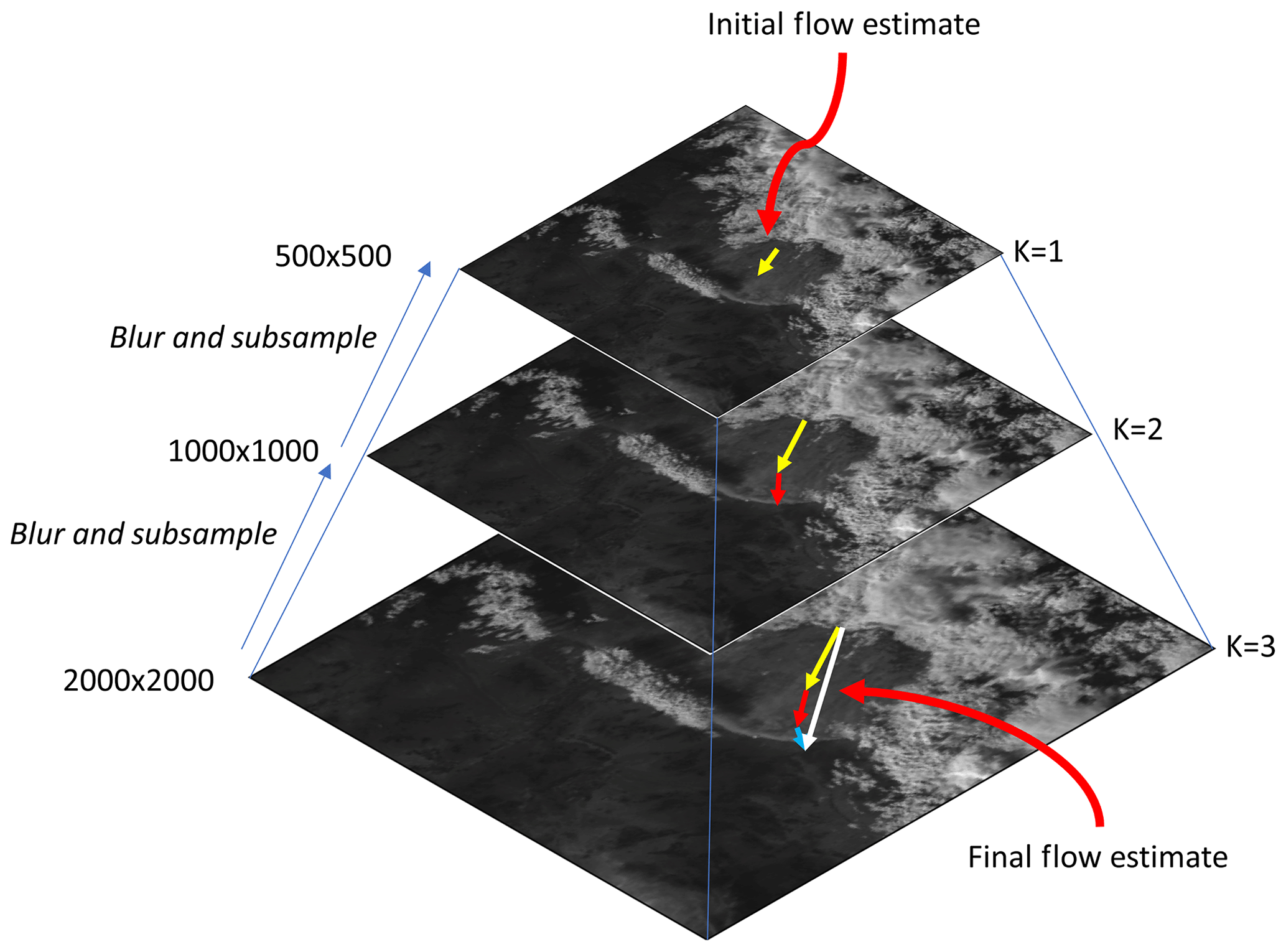
Figure 3 Schematic of coarse- to fine-scale warping optical flow in GOES imagery. The largest displacements are found in the initial coarse grid (yellow arrow at the top of the pyramid), which are used as initial displacements for the next levels (red and blue arrows). The final displacement is the sum of each displacement estimate (white arrow). In this schematic, an example scale factor of 0.5 was used over three pyramid levels; in this work, a scale factor of 0.95 for 77 levels was used.

Table 1 Settings used in the Brox et al. (2004) successive over-relaxation scheme.

Research and extensive validation have shown that, with quality control, PM provides a valuable resource to derive and identify winds in satellite imagery (Velden and Bedka, 2009). However, there are several types of motions for which PM would fail (Fig. 1b), many of which occur frequently in satellite OFB observations. AMVs found with Eq. (4) make two key assumptions: (1) that the brightness remains constant between sequential images at time t and t+Δt and (2) that the motion U is constant within the target. The first assumption, brightness constancy, fails when there are excessive illumination changes in a sector that are not due to motion. These illumination changes may be due to evaporation or condensation or simply due to changes in solar zenith angle throughout the day in visible imagery. The HS method also uses assumption (1), though it is relaxed when combined with the smoothness constraint. Assumption (2), which is not made in the HS method or other global methods, implies that the PM method has no way to handle rotation, divergence, or deformation in an efficient manner unless it is known a priori. Assumption (2) also fails to account for motion discontinuities, such as those near cloud edges or within transparent motions. Furthermore, as there is no other constraint aside from constant brightness, PM methods struggle when there is little to no texture in the target and candidates. Quality control schemes are thus necessary to remove sectors that are poorly tracked with Eq. (4) in most AMV approaches.

PM was a popular method for AMVs over other optical flow approaches prior to the GOES-R era due to its simplicity, computational efficiency, and capability to handle displacements common in low-temporal-resolution satellite imagery (Bresky and Daniels, 2006). Linearizing the brightness constancy assumption in Eq. (2) means that large and nonlinear displacements (typically > 1 pixel between images) will not be captured (Brox et al., 2004). Thus, most optical flow computations initially subsample images to the point at which all the displacements are initially less than 1 pixel (Anandan, 1989; discussed more in Sect. 3.1), which can cause fast-moving small features to be lost. Note that reducing the temporal resolution of GOES imagery (e.g., 10 min vs. 5 min scans) increases the displacement of typical meteorological features between frames. Furthermore, constancy assumptions are more likely violated with reduced temporal resolution since image intensity changes more through the evaporation and condensation of cloud matter over time. Thus, for the spatial resolution of ABI, it is impractical to consider optical flow gradient-based methods at temporal resolutions coarser than 5 min for several mesoscale meteorological phenomena, including OFBs. Very spatially coarse images do not need to be initially used with faster scanning rates, such as super rapid scan 1 min information (Schmit et al., 2013) or the 30 s temporal resolution mesoscale mode of ABI (Schmit et al., 2017).

While the HS method is designed for deriving dense flow in imagery sequences, it also does not account for motion discontinuities in the flow fields. Hence, it suffers from incorrect flow derivations near cloud edges and would perform poorly for OFB detection and tracking. Black and Anandan (1996) offer an intuitive solution to this problem, whereby the energy functional is designed to minimize robust functions that are not sensitive to outliers.

$$\begin{array}{}\text{(5)}& E\left(\mathbf{U}\right)=\int \underset{\mathrm{\Omega }}{\int }{\mathit{\rho }}_d\left(\mathrm{\nabla }I\cdot \mathbf{U}+I_{\mathrm{t}}\right)+{\mathit{\rho }}_{\mathrm{s}}\left(\mathrm{|}{\mathrm{\nabla }}_{\mathrm{2}}u{\mathrm{|}}^{\mathrm{2}}+\mathrm{|}{\mathrm{\nabla }}_{\mathrm{2}}v{\mathrm{|}}^{\mathrm{2}}\right)\mathrm{d}\mathit{x}\end{array}$$

The robust function data term for the HS method is simply ρ_d(r)=r² and smoothness ρ_s(r)=r, which implies that energy functionals increase quadratically for r outliers. Other robust functions can also be minimized with similar gradient descent algorithms to Gauss–Seidel iterations, while being less sensitive to outliers (Press et al., 1992; Black and Anandan, 1996). Robust functions are popular in recent optical flow literature (Brox et al., 2004; Sun et al., 2014), and a similar approach adopted here is discussed further in the Methodology section. The reader is referred to works by Barron et al. (1994), Fleet and Weiss (2005), Sun et al. (2014), and Fortun et al. (2015) for more comprehensive reviews on optical flow background and techniques.

The relevance of optical flow in satellite meteorological research continues to increase now that scanning rates of sensors such as the ABI are routinely at sub-5 min timescales, making motion easier to derive objectively (Bresky and Daniels, 2006; Héas et al., 2007; Wu et al., 2016). The dense motion estimation within fine-temporal-resolution data has yet to be used for feature identification. Optimizing optical flow for this purpose, and its specific application to OFBs, is the aim of this study. The next section outlines our approach to this end.

3 Methodology

3.1 Optical flow approach

As recently overviewed in Fortun et al. (2015), there are several optical flow approaches that provide dense motion estimates that account for the weaknesses highlighted in Fig. 1b. Many have their own advantages and drawbacks in terms of computational efficiency, flexibility, and capability to handle large displacements, motion discontinuities, texture-less regions, and turbulent scenes. We selected an approach here by Brox et al. (2004) (Hereafter B04), given its simplicity, current availability of open-source information, and excellent documentation. The reader is cautioned, however, that dense optical flow is a rapidly evolving field, and research is currently underway to improve present techniques. While dense optical flow validation for satellite meteorological application research like OFB identification is taking place, the reader is referred to the Middlebury (Baker et al., 2011), the MPI Sintel (Butler et al., 2012), and the KITTI (Geiger et al., 2012) benchmarks for extensive validation statistics of the most recent techniques using image sequences for more general applications.

The B04 approach handles the drawbacks described in Fig. 1b and more, whereby the brightness constancy assumption is no longer linearized, i.e.,

$$\begin{array}{}\text{(6)}& \begin{array}{rl}E\left(\mathbf{U}\right)& =\int \underset{\mathrm{\Omega }}{\int }{\mathit{\rho }}_d\left({\left|I\left(\mathit{x}+\mathbf{U},t+\mathrm{\Delta }t\right)-I\left(\mathit{x},t\right)\right|}^{\mathrm{2}}\right.\\ & \left.+\mathit{\gamma }{\left|{\mathrm{\nabla }}_{\mathrm{2}}I\left(\mathit{x}+\mathbf{U},t+\mathrm{\Delta }t\right)-{\mathrm{\nabla }}_{\mathrm{2}}I\left(\mathit{x},t\right)\right|}^{\mathrm{2}}\right)\\ & +\mathit{\alpha }{\mathit{\rho }}_{\mathrm{s}}\left(\mathrm{|}{\mathrm{\nabla }}_{\mathrm{2}}u{\mathrm{|}}^{\mathrm{2}}+\mathrm{|}{\mathrm{\nabla }}_{\mathrm{2}}v{\mathrm{|}}^{\mathrm{2}}\right)\mathrm{d}\mathit{x}.\end{array}\end{array}$$

Following B04, within the data robust function, we now have also included a gradient constancy assumption, which is weighted by a constant γ to make the derived flow more resilient to changes in illumination. Avoiding linearization of constancy assumptions improves the identification of large displacements between images. The Charbonnier penalty is used for the data and smoothness robust functions following Sun et al. (2014),

$$\begin{array}{}\text{(7)}& {\mathit{\rho }}_d\left(r^{\mathrm{2}}\right)={\mathit{\rho }}_{\mathrm{s}}\left(r^{\mathrm{2}}\right)=\sqrt{r^{\mathrm{2}}+{\mathit{ϵ}}^{\mathrm{2}}},\end{array}$$

with ϵ representing a small constant present to prevent division by zero in minimization, set to 0.001. The values for U are found by solving the Euler–Lagrange equations of Eq. (6) with numerical methods:

$$\begin{array}{}\text{(8)}& {\displaystyle }{E}_u-{\displaystyle \frac{\mathrm{d}{E}_{u_x}}{\mathrm{d}x}}-{\displaystyle \frac{\mathrm{d}{E}_{u_y}}{\mathrm{d}y}}=\mathrm{0},\text{(9)}& {\displaystyle }{E}_v-{\displaystyle \frac{\mathrm{d}{E}_{v_x}}{\mathrm{d}x}}-{\displaystyle \frac{\mathrm{d}{E}_{v_y}}{\mathrm{d}y}}=\mathrm{0},\end{array}$$

with reflecting boundary conditions and subscripts that imply the derivatives. Equations (8) and (9) are solved with a nested fixed-point successive over-relaxation iteration scheme described in B04 and summarized in Fig. 2. The reader is referred to Chap. 4 of Brox (2005) for details on the full discretization of the derivatives in the successive over-relaxation scheme. Here, only the spatial dimensions are used for the smoothing term, though it is possible to include the time dimension with this system as well.

A difficulty in solving Eqs. (8) and (9) is that the successive over-relaxation scheme may converge on a local minimum of E(U) rather than finding the global minimum. The typical approach to find the global minimum is to compute optical flow with coarse- to fine-scale warping iterations (e.g., Anandan, 1989). Coarse- to fine-scale warping iterations work by subsampling the initial image at the native resolution to a coarser spatial resolution and computing the flow initially at the coarsest resolution in the image pyramid. The U results from the coarse image flow are then used as the first-guess field for the next finest scale on the image pyramid (Fig. 3), and the second image is warped accordingly. The warping step ensures that estimated displacements at every step in the image pyramid remain small.

The B04 scheme includes coarse- to fine-scale warping iterations at every outer iteration k. This means that the first iteration is run on a subsampled image, and the subsampling is reduced by a scale factor at every k until the image reaches the native resolution at the final k=nK. Images at every k in this subsampling are found using a Gaussian image pyramid technique with bicubic interpolation. The flow values of the image at k−1 are also upscaled accordingly at k with bicubic interpolation (the initial flow guess is $u=v=\mathrm{0}$ at k=0). For improved computation of spatial derivatives, the initial image is also smoothed with a 9×9 pixel kernel Gaussian filter with a standard deviation set to 1.5 pixels. The specific settings used for the coarse- to fine-warped flow scheme here are shown in Table 1.

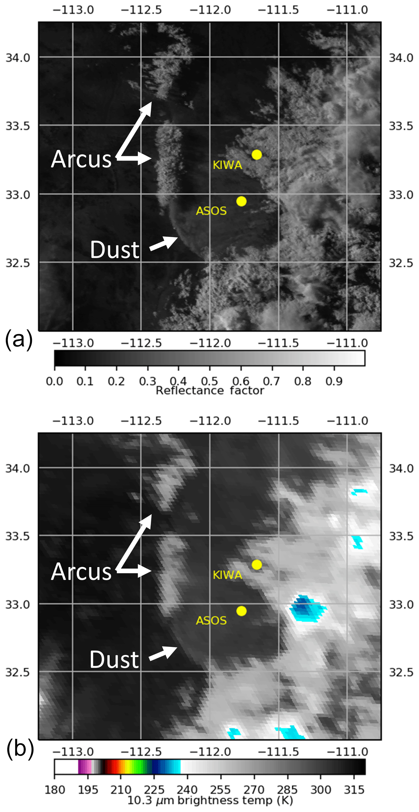
Figure 4 The 6 July 2018 00:23 UTC GOES-16 0.64 µm visible reflectance (a) and BT_10.35 (b) over south–central AZ, centered on an OFB of interest.

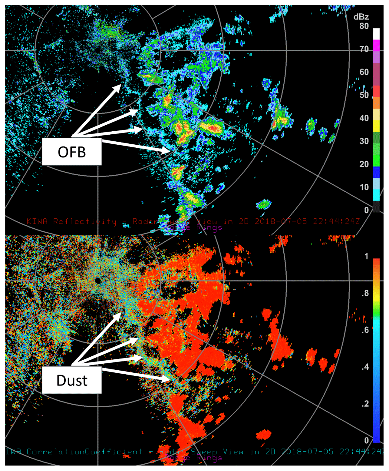
Figure 5 The KIWA radar 22:44 UTC 0.5^∘ horizontal reflectivity (top; dBZ) and correlation coefficient (bottom). Range rings in grey indicate every 30^∘ azimuth and 50 km in range.

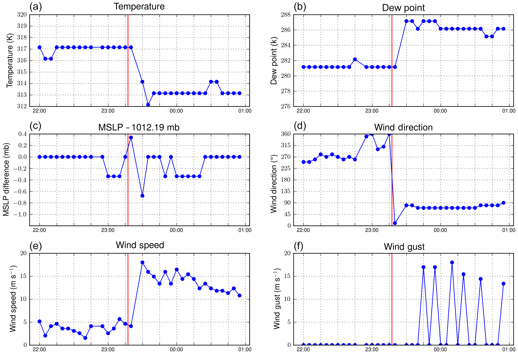
Figure 6 Surface high-frequency METAR observations of temperature (K; a), dew point (K; b), mean sea level pressure (middle c), wind direction (^∘ from N; d), wind speed (m s⁻¹; e), and wind gusts (m s⁻¹; f). The surface station was located at (32.95^∘ N–111.77^∘ E). The red line indicates the approximate time of boundary passage over the station.

3.2 Objective OFB identification

There are two steps to the objective OFB identification process. First, a linear feature or sharp boundary is identified in visible or infrared imagery. In some cases, the first step alone is enough to identify OFBs subjectively. The second step is tracking that feature back in time to see where it originated from (typically, near an area with deep convection). In the case of near-stationary convection and low-level flow, a forecaster might also use radial-like propagation in this decision-making process; however, since convection geometry and low-level flow vary from storm to storm, only the first two steps are considered here. This approach aims to mirror the subjective process, leveraging the information content of optical flow to do so.

To handle the first step of line feature identification, a simple image line detection scheme was performed by convolving the original brightness field with a set of line detection kernels, so

$$\begin{array}{}\text{(10)}& L=\sum _{i=\mathrm{1}}^{\mathrm{4}}{\mathbf{a}}_i\star G\left(R\right),\end{array}$$

where ⋆ is the convolution operator, G is a Gaussian smoothing function (using a 21×21 kernel and standard deviation of 5 pixels), R is the reflectance factor (radiance times the incident Lambertian-equivalent radiance, or the “kappa factor”; Schmit et al., 2010), L is the resulting line detection field, and a_i represents the two-dimensional line detection kernels defined as follows.

$$\begin{array}{rl}& {\mathbf{a}}_{\mathrm{1}}=\left[\begin{array}{ccc}-\mathrm{1}& -\mathrm{1}& -\mathrm{1}\\ \mathrm{2}& \mathrm{2}& \mathrm{2}\\ -\mathrm{1}& -\mathrm{1}& -\mathrm{1}\end{array}\right]\\ & {\mathbf{a}}_{\mathrm{2}}=\left[\begin{array}{ccc}-\mathrm{1}& \mathrm{2}& -\mathrm{1}\\ -\mathrm{1}& \mathrm{2}& -\mathrm{1}\\ -\mathrm{1}& \mathrm{2}& -\mathrm{1}\end{array}\right]\\ & {\mathbf{a}}_{\mathrm{3}}=\left[\begin{array}{ccc}\mathrm{2}& -\mathrm{1}& -\mathrm{1}\\ -\mathrm{1}& \mathrm{2}& -\mathrm{1}\\ -\mathrm{1}& -\mathrm{1}& \mathrm{2}\end{array}\right]\\ & {\mathbf{a}}_{\mathrm{4}}=\left[\begin{array}{ccc}-\mathrm{1}& -\mathrm{1}& \mathrm{2}\\ -\mathrm{1}& \mathrm{2}& -\mathrm{1}\\ \mathrm{2}& -\mathrm{1}& -\mathrm{1}\end{array}\right]\end{array}$$

The resulting L field exhibits higher intensities wherein line features exist (Gonzalez and Woods, 2007). A threshold of L≥0.02 was used here to indicate that a pixel contained a line feature. This method was compared to a subjective interpretation of boundary location for validation.

To address the second step of the process, the constrained optical flow approach described in Sect. 3.1 was used to track the boundary pixels (both objectively and subjectively identified) back in time for 3 h. The values of motion at each step in the backwards trajectory were determined with bilinear interpolation of the optical-flow-derived dense vector grid. If a back-traced pixel of the linear feature arrived within a 50 km great-circle distance of a 10.35 µm brightness temperature (BT_10.35) pixel lower than 223 K (−50 ^∘C; using previous satellite imagery matched to the back-trajectory time), the original point was considered an OFB. The area subtended by the 50 km great circles derived from BT_10.35 is hereafter referred to as the “deep convection area.” While this brightness temperature threshold is subjective and can vary from case to case, it was found to produce a reasonable approximation of deep convection areas when compared to ground-based radar information for the case study described in the subsequent sections.

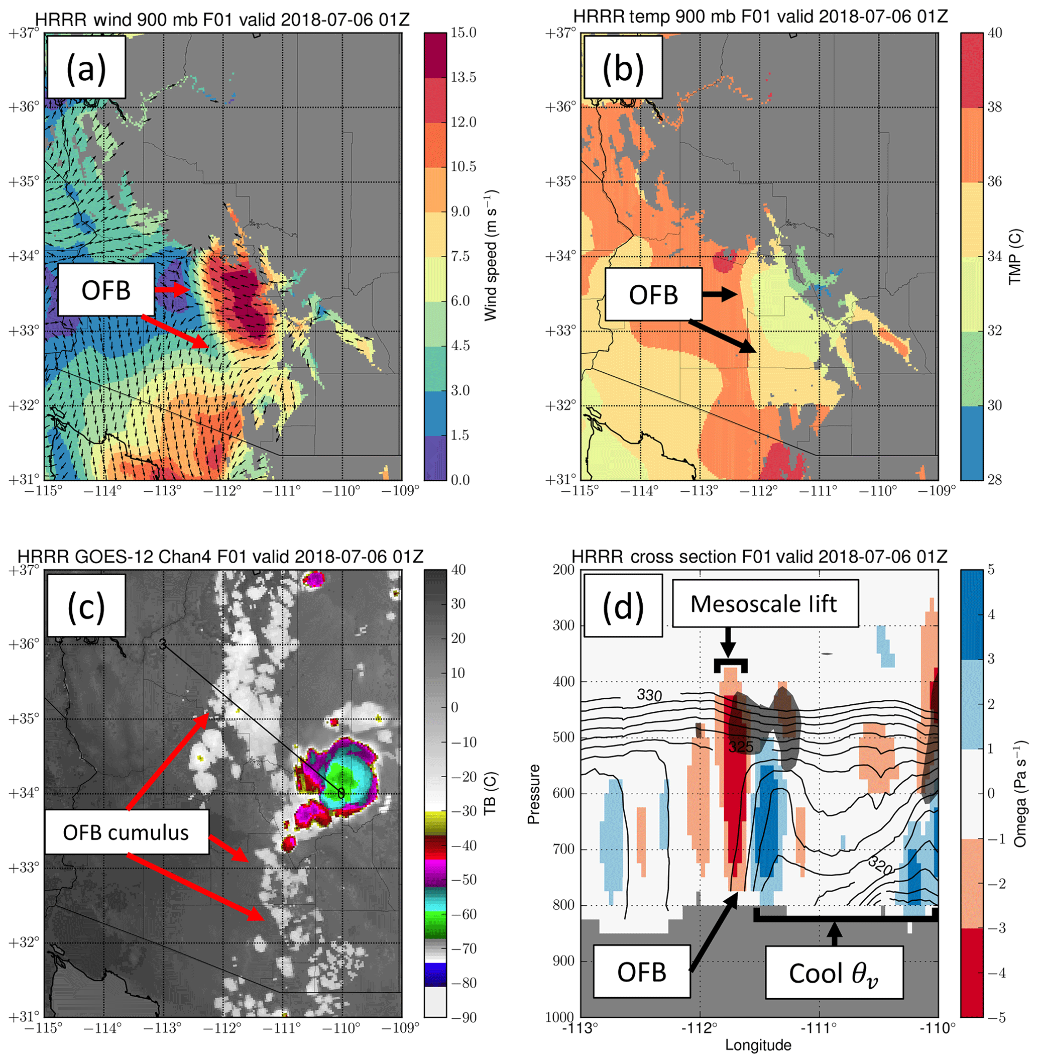
Figure 7 HRRR output of an OFB event, including (a) wind speed, (b) temperature, (c) simulated infrared brightness temperature, and (d) a cross section along the black line in (c) with virtual potential temperature θv in black contours (K), omega in color-shaded pixels, and regions of relative humidity > 90 % highlighted with dark shading (bottom right).

3.3 Data

The objective OFB identification methodology is tested using a case study from 5 July 2018 over the southwestern United States. This event featured a distinct OFB and associated dust storm that was well-sampled by various ground- and space-based sensors. GOES-16 was in mode 3, generating one image over the study area every 5 min (continental US, or CONUS, ABI scan domain, NOAA, 2019). Optical flow computations employ the GOES-16 (GOES-East) ABI red band (0.64 µm; ABI channel 2), provided at a nominal sub-satellite spatial resolution of 500 m, but closer to 1 km at the case study location. This channel is used at native resolution, though it can be subsampled with a low-pass filter such that future versions can implement color information from the blue and near-infrared bands (e.g., Miller et al., 2012). This means that the optical flow approach here is daytime only. A similar B04 approach can be used on infrared data as well for day–night independent information, though for detecting OFBs in the low levels, proxy visible products would perform best. As described above, the clean longwave infrared band (10.35 µm; ABI channel 13) is used as first-order information on optically thick cloud-top heights and to assess the convective nature of the observed scene (BT_10.35 < 223 K).

High-frequency Automated Surface Observing Stations (ASOSs; NOAA, 1998), recording temperature, pressure, wind speed, and direction once every minute, complement the satellite imagery. The Weather Surveillance Radar-1988 Doppler (Crum and Alberty, 1993) dual-polarimetric data also sampled the OFB event from the KIWA radar near Phoenix, AZ. To highlight the OFBs and the presence of dust, horizontal reflectivity and the correlation coefficient are used (Van Den Broeke and Alsarraf, 2016). Finally, for information on the full 3D dynamics of the case study, a numerical model representation of the environment was collected from the High Resolution Rapid Refresh system (HRRR; Benjamin et al., 2016). The combination of these model and observation datasets is employed to confirm the presence of a distinct convective OFB rather than some other quasi-linear feature, such as a bore or elevated cloud layer.

Figure 8 The 00:23 UTC GOES-16 0.64 µm visible channel shown with a (a) subjectively identified OFB (blue dots) and (b) linear feature L≥0.02 field (blue shading). Also shown are linear features that contained fast storm-relative motion (red shading). The results of backtracking the (c) subjectively and (d) objectively identified OFB features are also shown; blue dots represent targets tracked back within 50 km of a deep convection event, and orange dots are targets that were not.

4 Case study description

Convection was observed in south–central Arizona on 5 July 2018 after 18:00 UTC. A large and well-defined linear structure emerged from below the convective cloud cover at 22:00 UTC to 6 July 2018 01:00 UTC propagating westward in GOES-16 imagery (Fig. 4). This linear structure, demarcated by roll (arcus) clouds on the northern side and lofted dust on the southern side, was apparent with strong visible reflectance contrast against the relatively dark surface and BT_10.35 ∼10 K cooler than the underlying surface. The dust lofted by this outflow produced low visibility and hazardous driving conditions near Phoenix, AZ. Dust storm warnings were issued by the local National Weather Service (NWS) forecast office by 23:00 UTC. The structure's observed radial propagation away from nearby deep convection and associated cloud and dust features contributes to its interpretation as a convective OFB.

The OFB was also captured in radar scans from KIWA at 22:00 UTC (Fig. 5). The coincidence of a low correlation coefficient (< ∼0.5) and moderate to high reflectivity (near 20 dBZ) implies that the OFB contained non-meteorological scatterers (e.g., Zrnic and Ryzhkov, 1999). The radar measurements are consistent with previous reported values of lofted dust (Van Den Broeke and Alsarraf, 2016). Surface observations taken at the ASOS reveal temperatures exceeding 317 K (44 ^∘C) ahead of the OFB, with calm winds (Fig. 6). Temperatures dropped by 4 K, wind speeds changed direction and increased sharply, and dew points increased rapidly as the OFB crossed the station at ∼23:16 UTC. The rapid change in low-level meteorology is consistent with convective OFBs sampled in previous studies (e.g., Mahoney, 1988; Miller et al., 2008).

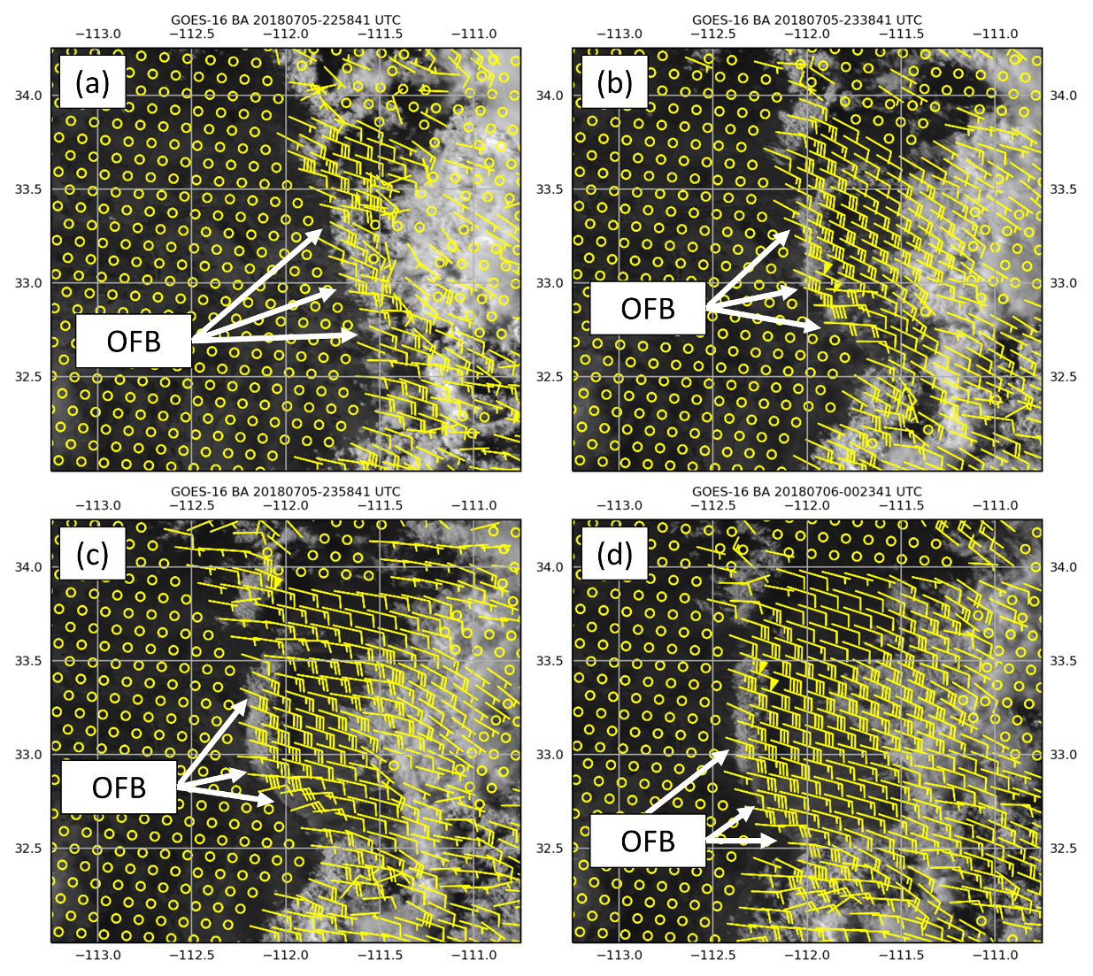
Figure 9 GOES-16 0.64 µm visible channel imagery on 5 July 2018 at (a) 22:58 UTC, (b) 23:38 UTC, (c) 23:58 UTC, and (d) 00:23 UTC over central Arizona shown with every 20th optical flow vector in the x and y directions (subsampled for image clarity) illustrated with yellow wind barbs (knots). Circles represent motion < 5 kn, which commonly occurs over ground pixels.

The HRRR model captured the broad characteristics of this event (Fig. 7), showing moderate low-level winds in excess of 10 m s⁻¹ (Fig. 7a), cooler temperatures (Fig. 7b), and simulated cumulus clouds from forced ascent (Fig. 7c). Model cross sections (Fig. 7d) indicated a moderate increase in vertical motion ahead of the numerically derived boundary and a sharp decrease in virtual potential temperature behind the boundary. The shape of the virtual potential temperature profile is consistent with other model observations of OFBs (e.g., Chipilski et al., 2018). The observation and model data all show that the linear structure observed in Fig. 4 was modifying the dynamics of the surface in a manner consistent with OFBs and not some other linear cloud feature type that is decoupled from the surface and may be misidentified by the satellite. Since such low-level linear features are often obscured by cloud layers at higher altitudes, this case study in some respects represents a best-case scenario for evaluating optical flow capabilities towards identifying OFBs.

5 Results

The first step in OFB identification requires the identification of a feature that appears linear in the imagery. Compared to the subjective boundary identification (considered truth here; Fig 8a, blue dots), the convolution method gives a reasonable approximation of where the OFB is located within the higher-intensity points in L (Fig. 8b). Unfortunately, the simply applied convolution is also sensitive to linear features associated with the deep convection itself (the blue shading in Fig. 8b). Hence, false alarms appear east of the boundary. These issues can be filtered out using either cloud-top height or brightness temperature thresholding from separate infrared channels. Alternatively, the storm-relative motion (here > 15 m s⁻¹), or the motion relative to the 6 h forecast field of 0–6 km storm motion from the Global Forecast System (GFS) numerical weather prediction model run, was used here to filter the false alarms (the red shading in Fig. 8b). The GFS forecast field was used over analysis to simulate what would be available globally in real time.

The second step requires these linear fast-moving features to be traced backward to a deep convection source using the optical flow computation (Fig. 9). To the west of the boundary, near-stationary optical flow vectors highlight the background (or ground) pixels. The boundary itself exhibits a westward movement near 15–20 m s⁻¹ (∼30–40 kn). The feature also appears to bow outwards after faster motions are observed (near 33^∘ N, −112^∘ E) during 23:38–23:58 UTC (Fig. 9b, c). Similar westward motion is derived in the wake of the OFB, within the convective cold pool. This results from the presence of airborne dust particles, which facilitate the computation of optical flow vectors in this region.

The backwards trajectories of the subjectively and objectively identified OFB pixels in Fig. 8c and d (B04 method) show that many of the linear cloud features, particularly those associated with the central arcus cloud, indeed originated near deep convection. However, when the backwards trajectories of the B04 method were compared to other optical flow methods, such as the approach by Wu et al. (2016), most were unsuccessful at obtaining coincidence between linear cloud features along the OFB and a deep convection source. Wu et al. (2016) used an approach introduced to the community by Farnebäck (2001), which is a local window method for optical flow.

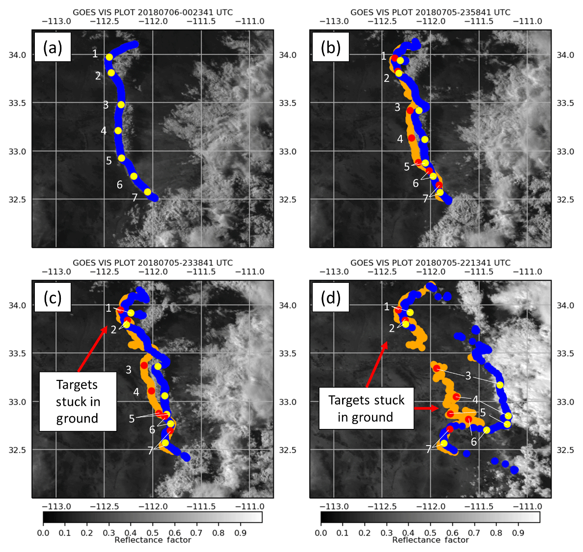
Figure 10 The GOES-16 0.64 µm visible imagery shown with image targets backtracked from subjective identification in Fig. 8a at 00:23 UTC 6 July 2018 using the B04 method (blue–yellow) and the Wu et al. (2016) approach (orange–red) at (a) 00:23 UTC, (b) 23:58 UTC, (c) 23:38 UTC, and (d) 22:13 UTC. Individual points are highlighted from each approach (yellow and red dots; see text).

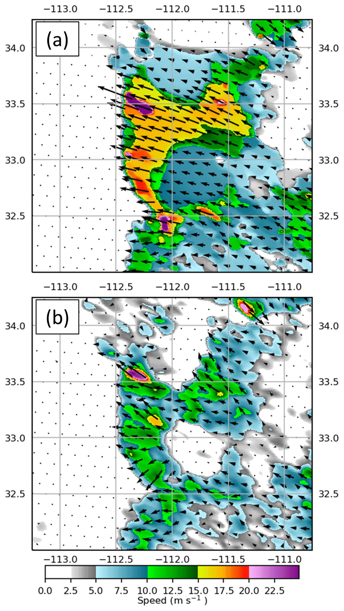
Figure 11 Color-shaded wind speed for 00:23 UTC 6 July 2018 over central Arizona from (a) the B04 optical flow method and (b) the Wu et al. (2016) flow, shown with respective flow vectors and the subjective position of the front edge of the OFB (blue line).

Example points 1–7 examined within the subjectively identified OFB backward trajectories highlight an issue with local window approaches for this application (Fig. 10). The B04 approach (Fig. 10, blue–yellow) produced motions that were relatively consistent with the true boundary motion. Thus, many points that are lost in the local approaches are successfully backtracked to the initial deep convection (e.g., points 3–5). With the Wu et al. approach (Fig. 10, orange–red), OFB targets move slower than the actual boundary and, over a 3 h tracking period, eventually become stuck within the stationary background pixels. This tracking issue stems from an assumption made in many local approaches that pixels within an image window all move in the same direction with the same speed. When background pixels are included within an image window containing clouds or dust, the resulting optical flow speed would then be underestimated. The slow bias is observed in plots of optical flow speeds along the OFB (Fig. 11), for which the Wu et al. approach was ∼5–10 m s⁻¹ slower than the B04 approach. While not shown, we found similar backward trajectory issues using the LK approach. Full loops of the optical flow in Fig. 9 and trajectories in Fig. 10 are included in the Supplement to this paper.

For all approaches tested, however, the methods struggled to backtrack the newly formed cumulus to the north and the dust front to the south. With the cumulus to the north, the issues with each algorithm appear to result from rapid cumulus development between frames (e.g., points 1 and 2 in Fig. 10a, b). Condensation like what is observed here is unfortunately not considered in the brightness constancy assumption. Thus, condensing cloud features would only be tracked back to when they initially form (after Fig. 10b) without additional dynamic constraints to Eq. (6). An example can be seen when points 1 and 2 become stuck in Fig. 10c. This has important implications for the limitations of backtracking OFB features to deep convection with optical flow from imagery. If no cloud or dust feature exists to visualize an OFB in satellite imagery, some of the feature propagation may be lost.

The dust to the south appears in the satellite imagery as early as 22:00 UTC, though it was quite transparent relative to the ground. It is therefore possible the stationary background pixels may be dominant in the optical flow computation at points 6 and 7, resulting in slower wind speeds than the true OFB propagation. Points 6 and 7 are also located near cumulus moving across the OFB motion to the south. This dust front tracking could be improved using multispectral techniques designed to highlight dust features over ground pixels or by using additional color spectrum information to discourage flow smoothness in Eq. (6) across the dust front from the cumulus to the south (e.g., Sun et al., 2014).

Many line-like targets east of the OFB in Fig. 8d also originated from the deep convection, which constitute false alarms. These false alarms can be reduced by further improving the OFB targeting step in the objective process in future studies. For this case study, it may have been possible to use convergence thresholding methods, analogous to radar-based objective OFB identification, to isolate the boundary. However, convergence as derived from the optical flow information here would only work because of local, stationary surface pixels ahead of the OFB. Thus, convergence would be stronger with faster OFB velocity, which is undesirable for an objective identification product as slow-moving OFBs would be missed. The convergence would also be sensitive to nearby cloud structures ahead of the OFB, which would exhibit different (nonstationary) motion from the surface. It is for this reason that a backwards trajectory approach was selected instead of basing the detection on local horizontal convergence. The optical flow approach used here does help highlight the OFB when storm motion alone was considered in addition to convolution, showing how additional tools can be used in synergy to arrive at a more comprehensive objective feature identification approach in future studies.

6 Conclusions and future outlook

A new method for the objective identification of outflow boundaries (OFBs) in GOES-16 Advanced Baseline Imager (ABI) data was developed using optical flow motion derivation algorithms and demonstrated with provisional success on a dust storm case study. An optical flow system constructed for this purpose shows promise in identifying and backtracking object events to their source over traditional flow derivation methods, which can potentially be used to isolate convective OFB features. To the best of the authors' knowledge, this study represents a first attempt to objectively identify OFBs in geostationary satellite imagery.

The primary conclusion of this study is that optical flow approaches are now a viable option to acquire mesoscale flows relevant to OFB tracking and detection in 5 min geostationary satellite imagery, though the successful backtracking of OFB features requires the use of flow algorithms that can handle the presence of motion discontinuities and stationary background flow. The optical flow algorithm tested in this study produced a dense motion field that was closer than other methods to the true OFB motion and provided valuable information towards full objective OFB identification in new products.

While several OFB-related image pixels were successfully identified, the algorithm here is relatively immature and remains fraught with false alarms, whereby linear features are incorrectly identified and correct features were not successfully backtracked to deep convection. The algorithm is still limited by the assumptions made within optical flow, which only account for changes in image brightness intensity resulting from pure feature advection. Therefore, if no features (e.g., clouds) exist to highlight an OFB boundary within the imagery, the method proposed here would not function properly. The method also struggles to resolve true OFB motions with transparent dust movement, for which a textured background beneath the dust may dominate the motion estimate within a scene. Also, while infrared brightness temperature was enough to identify deep convection in this case study, convection may be missed by brightness temperature imagery if it is obscured by a higher cloud layer or if the minimum cloud-top brightness temperature exceeds an arbitrarily set threshold.

Given these limitations, future studies will explore more advanced systems for linear structure identification to identify candidate features for tracking towards full objective OFB identification. A machine-learning system will be used to determine which linear characteristics of the image should be backtracked instead of using two-dimensional convolution. Optical flow can be used to precondition training information for a machine-learning approach if the motion or semi-Lagrangian fields are needed. Furthermore, it will be prudent to use deep convection correspondence through optical flow backtracking as one of many fields in future products, such as radial propagation away from storms and near-surface meteorological properties, to probabilistically decide if an image pixel is associated with an OFB. To better identify deep convection areas, the GOES Lightning Mapper (GLM) can be used, which provides information on lightning location and energy at 8 km resolution with a 2 ms frame rate.

Feature identification with optical flow is not restricted to OFBs alone. For example, the above-anvil cirrus plume (Bedka et al., 2018) over deep convection has been identified as an important indicator of severe weather at the ground, yet no objective means of identification exists today. The properties from optical flow could be used as an additional source of information in such algorithm designs, allowing researchers to backtrack features to their apparent source (the overshooting top in the case of the above-anvil cirrus plume) and monitor cloud temperature and visible texture trends or to simply use the dense motion itself to achieve better results. This method will also be applicable to other cold pool outflow phenomena, such as bores, for which new algorithms could utilize numerical model or surface observations for further clarification of linear feature type.

Motion-discontinuity-preserving optical flow will also benefit several current algorithms for monitoring deep convection in satellite imagery. Objective deep convection cloud-top flow field algorithms (Apke et al., 2016, 2018) will particularly benefit when sharp cloud edges and ground pixels are present in an image scene. Systems that use infrared cloud-top cooling or emissivity differences for deep convection nowcasting will also improve with better estimates of pre-convective cumulus motion (Cintineo et al., 2014; Mecikalski and Bedka, 2006).

While the utility of a backwards trajectory approach was considered here, many other possible methods exist for exploiting the semi-Lagrangian properties of time-resolved observations in satellite imagery (e.g., Nisi et al., 2014). The use of fine-temporal-resolution information will improve optical flow estimates and in turn the estimates of brightness temperature, reflectance, or cloud property changes in a moving frame of reference. We will explore these and other refinements in ongoing and future work on this exciting frontier of next-generation ABI-enabled science.