Discrete-wavelength DOAS NO₂ slant column retrievals from OMI and TROPOMI

The use of satellite NO₂ data for air quality studies is increasingly revealing the need for observations with higher spatial and temporal resolution. The study of the NO₂ diurnal cycle, global sub-urban-scale observations, and identification of emission point sources are some examples of important applications not possible at the resolution provided by current instruments. One way to achieve increased spatial resolution is to reduce the spectral information needed for the retrieval, allowing both dimensions of conventional 2-D detectors to be used to record spatial information.

In this work we investigate the use of 10 discrete wavelengths with the well-established differential optical absorption spectroscopy (DOAS) technique for NO₂ slant column density (SCD) retrievals. To test the concept we use a selection of individual OMI and TROPOMI Level 1B swaths from various regions around the world, which contain a mixture of clean and heavily polluted areas. To discretise the data we simulate a set of Gaussian optical filters centred at various key wavelengths of the NO₂ absorption cross section. We perform SCD retrievals of the discrete data using a simple implementation of the DOAS algorithm and compare the results with the corresponding Level 2 SCD products, namely QA4ECV for OMI and the operational TROPOMI product.

For OMI the overall results from our discrete-wavelength retrieval are in very good agreement with the Level 2 data (mean difference <5 %). For TROPOMI the agreement is good (mean difference <11 %), with lower uncertainty owing to its higher signal-to-noise ratio. These discrepancies can be mostly explained by the differences in retrieval implementation. There are some larger differences around the centre of the swath and over water. While further research is needed to address specific retrieval issues, our results indicate that our method has potential. It would allow for simpler, more economic satellite instrument designs for NO₂ monitoring at high spatial and temporal resolution. Constellations of small satellites with such instruments on board would be a valuable complement to current and upcoming high-budget hyperspectral instruments.

1 Introduction

Nitrogen dioxide (NO₂) is a gaseous air pollutant from the NO_x family (${\mathrm{NO}}_x=\mathrm{NO}+{\mathrm{NO}}_{\mathrm{2}}$) that exists in trace amounts in the atmosphere. Its sources are of natural origin (e.g. lightning, volcanoes, and microbial activity) or a result of anthropogenic activities (e.g. agricultural biomass burning, fossil fuel combustion). Most of the background NO₂ is in the stratosphere and is produced mainly by natural processes. However, in polluted areas tropospheric NO₂ is predominant and its main sources are anthropogenic emissions, which occur close to the surface in the boundary layer. Other sources of tropospheric NO₂ include fires, microbiological soil emissions, and lightning (Wallace and Hobbs, 2006).

The most polluted regions are usually highly industrialised and densely populated urban areas, where the air pollution is complex due to the varied mix of constituents (Monks et al., 2009). There is evidence suggesting that NO₂ is a good proxy for the spatial variability of outdoor air pollution in urban environments (e.g. Levy et al., 2013), making it a suitable indicator of air quality.

NO₂ itself has harmful effects on human health, being associated for example with respiratory damage and premature death (WHO Regional Office for Europe, 2013). Moreover, it indirectly plays a role in the climate as it is a precursor of tropospheric ozone and aerosol, two of the essential climate variables defined by the Global Climate Observing System (GCOS) (WMO, 2011).

There has been a continuous effort, particularly in recent decades, to regulate and monitor the concentrations of air pollutants such as NO₂ with the aim of (a) reducing emissions and (b) putting in place mitigation strategies to minimise the exposure of people to harmful levels. Nonetheless, despite a general decreasing trend on NO₂ concentrations in many locations across the globe, particularly in Europe and the United States (e.g. Castellanos and Boersma, 2012; Russell et al., 2012), the World Health Organization (WHO) recommended limits for air quality (WHO, 2006), and EU legislative limits in the case of Europe (EEA, 2018), are still often exceeded (e.g. DEFRA, 2018). In addition, in other areas of the world such as China and India concentrations of nitrogen oxides continued to rise until less than a decade ago (e.g. Huang et al., 2017; Richter et al., 2005; Hilboll et al., 2017). This highlights that there is still a lot to do to tackle the problem of air pollution and that a reliable, consistent long-term monitoring network is crucial.

There are two main methods for the continuous observation of NO₂ in the atmosphere: in situ measurements and remote sensing techniques, which include ground-based and space-borne observations. In situ instruments such as chemiluminescence analysers (EPA, 1975; Dunlea et al., 2007) provide more accurate values because they directly measure the air they sample. However, it is not logistically or economically viable to install a large number of these around cities, so measurement points are usually sparse. Low spatial sampling is also a limitation of ground-based remote sensing (e.g. Network for the Detection of Atmospheric Composition Change, NDACC, http://ndaccdemo.org/, last access: 1 April 2020; Pandonia Global Network, PGN, https://www.pandonia-global-network.org, last access: 1 April 2020), but they provide long-term quality observations that can be used to validate satellite measurements. On the other hand, satellite instruments provide global coverage but the spatial and temporal resolution is limited, e.g. 3.5 km × 5.5 km (at nadir) once per day for TROPOMI (Veefkind et al., 2012), and retrieving surface concentrations of NO₂ from satellite platforms is not straightforward. Increased spatio-temporal resolution (ultimately in the range of 1 km × 1 km) is required to improve the accuracy of emission estimates and pollution forecasts (Ingmann et al., 2012).

NO₂ has typically been retrieved from measured earthshine spectra using the well-established differential optical absorption spectroscopy (DOAS;  Platt and Stutz, 2008) technique for over two decades, since the launch of GOME in 1995 aboard ERS-2 (Burrows et al., 1999). This was followed by SCIAMACHY (Bovensmann et al., 1999) aboard Envisat, OMI (Levelt et al., 2006) aboard Aura, GOME-2 (Munro et al., 2006) aboard MetOp-A, MetOp-B and MetOp-C, and more recently TROPOMI (Veefkind et al., 2012) aboard Sentinel-5P. Out of these, GOME-2, OMI and TROPOMI are still operational, and have a single daily overpass in the morning (GOME-2) or in the afternoon (OMI, TROPOMI). TROPOMI provides the best spatial resolution to date, with a true nadir ground pixel size as small as 3.5 km × 5.5 km, or 1.8 km × 1.8 km in the occasionally used zoom mode. Unlike their predecessors, OMI and TROPOMI have two-dimensional detectors that allow them to record multiple across-track viewing angles simultaneously (pushbroom measurement mode). While this mode results in higher spatial resolution, it comes at the cost of more optical complexity.

The DOAS principle relies on the separation of broadband and narrowband components of the reflectance spectrum and can resolve multiple gases simultaneously. DOAS retrievals typically use a few hundred spectral channels to perform the slant column density (SCD) fit for each ground pixel. The need for such a large number of channels requires complex optics, and careful wavelength calibration, for which the Fraunhofer lines in a reference solar spectrum are usually used. In addition, one dimension of the detector must be dedicated to recording all this spectral information.

One way to simplify instrument design and increase spatial resolution is to use a retrieval algorithm with reduced spectral information. The idea of using only a few discrete spectral channels to retrieve atmospheric trace gases has been used extensively for ozone retrievals. One example is the Total Ozone Mapping Spectrometer (TOMS; Heath et al., 1975), first launched in 1978 aboard Nimbus-7, which used pairs of discrete wavelengths in the Huggins band (310–340 nm) to retrieve ozone. Its strong, narrow absorption features and limited interference from other atmospheric gases make ozone a relatively easy species to retrieve using discrete wavelengths. For a weak absorber like NO₂, it is more challenging, but it has also been done using passive techniques, such as the Brewer spectrometer (e.g. Cede et al., 2006; Wenig et al., 2008) and the visible nitrogen dioxide instrument aboard the Solar Mesosphere Explorer (Mount et al., 1984), and active techniques, such as differential absorption lidar (DIAL; e.g. Hains et al., 2010). More recently, Dekemper et al. (2016) developed a new concept of an “AOTF-based NO₂ camera”, which employs pairs of wavelengths recorded sequentially using an acousto-optical tunable filter (AOTF) to image NO₂ in scenes containing plumes. However, these techniques lack sensitivity (e.g. Brewer) or rely on specific viewing geometries that make them unsuitable for nadir-viewing space applications. For example, the AOTF-based NO₂ camera relies on clear-sky pixels being present in the scene for background subtraction. In addition, the sequential sampling of wavelengths poses a limitation to the speed at which they can be registered, making the retrieval challenging for non-static scenes.

In this work we explore the development, application, and performance of a discrete-wavelength NO₂ retrieval algorithm based on DOAS (discrete-wavelength DOAS, DW-DOAS hereafter). Our approach combines the reduction in required spectral information with the advantages of DOAS in removing the effects of surface albedo, scattering, and interfering gases. As a proof of concept, we perform a feasibility study of the technique using data from OMI and TROPOMI and analyse the differences between our results and the operational Level 2 products. In addition, we discuss the implications of discretising DOAS and the potential application of our method to a future hypothetical instrument aimed at high-spatial-resolution urban air quality monitoring.

2 Method

2.1 Data sources

2.1.1 Ozone Monitoring Instrument (OMI)

The Ozone Monitoring Instrument (Levelt et al., 2006) is an ultraviolet–visible (UV/VIS) spectrometer and operational since it was launched in 2004 aboard the NASA AURA spacecraft. It is a nadir-viewing instrument and follows a sun-synchronous polar orbit, with a daily overpass of 13:45 LT (local time). The visible band covers a spectral range of 350–500 nm, with a spectral resolution of 0.63 nm and an average sampling distance of 0.21 nm. OMI has a nadir pixel size of 13 km × 24 km (13 km × 12 km in spatial zoom mode), with 60 across-track pixels covering a swath width of 2600 km.

OMI has had good in-flight performance so far, with only ∼0.5 % radiometric degradation in the visible channel in the 15 years it has been operational (Levelt et al., 2018). However, it does have one main issue, known as the “row anomaly” (described in detail in the KNMI OMI website: http://projects.knmi.nl/omi/research/product/rowanomaly-background.php, last access: 1 April 2020), affecting the quality of the radiance in specific rows of the detector. OMI data from 2009 onwards are affected by this anomaly, although early signs started to be seen in 2007. In the work presented here we use Level 1B data from 2005, which are not affected by the row anomaly.

Several OMI Level 2 NO₂ products have been produced by different institutions (e.g. NASA, Krotkov et al., 2017; KNMI, Boersma et al., 2011). In this work we use the product released as part of the Quality Assurance for Essential Climate Variables (QA4ECV) project (Boersma et al., 2017), which includes recent improvements in the retrieval algorithm (Boersma et al., 2018; Zara et al., 2018).

2.1.2 TROPOspheric Monitoring Instrument (TROPOMI)

Launched in 2017 aboard ESA’s Sentinel-5 Precursor, the TROPOspheric Monitoring Instrument (TROPOMI; Veefkind et al., 2012) is the state of the art in remote sensing of atmospheric composition, with heritage from OMI and SCIAMACHY. It is a pushbroom nadir spectrometer like OMI but it also covers the near infrared (NIR) and the shortwave infrared (SWIR). It flies in a sun-synchronous polar orbit with about the same daily local overpass as OMI. The visible band of interest in this study (band 4) covers a spectral range of 405–500 nm, with a spectral resolution of 0.55 nm and a spectral sampling of 0.2 nm. Along with an increased signal-to-noise ratio (SNR), one of the major advantages of TROPOMI is its unprecedented spatial resolution of 3.5 km × 5.5 km, which goes down to 1.8 km × 1.8 km in zoom mode. Like OMI, the swath width is 2600 km, but TROPOMI has 450 across-track pixels. In this study we use TROPOMI Level 1B data and the operational NO₂ Level 2 product (van Geffen et al., 2019).

2.2 Data processing

2.2.1 Processing chain

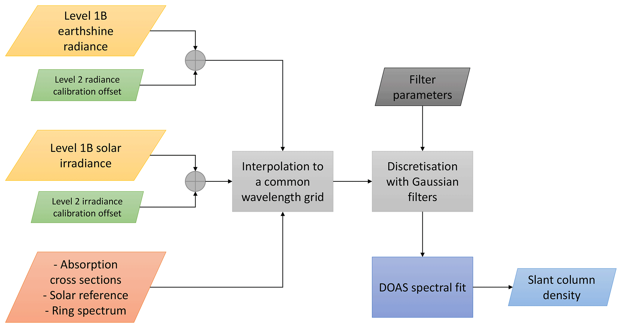
We simulate discrete-wavelength data by discretising OMI and TROPOMI Level 1B data using digital Gaussian filters. In addition, the relevant absorption cross sections, solar reference, and Ring spectrum, convolved with the corresponding row-dependent slit functions for either OMI or TROPOMI, are discretised. Before applying the filters, all the spectra are interpolated onto a common wavelength grid, selected according to what is used in the reference L2 products. Thus, for OMI we use the wavelength grid of the irradiance, and for TROPOMI, that of the radiance. We use a cubic spline interpolation for the cross sections. For the radiance and irradiance spectra we use the method employed by Bucsela et al. (2006), which calculates the interpolated spectrum using a high-resolution solar reference spectrum as follows:

$$\begin{array}{}\text{(1)}& F(\mathit{\lambda }+\mathrm{d}\mathit{\lambda })={\displaystyle \frac{F\left(\mathit{\lambda }\right)}{\left[F_{\mathrm{0}}\right(\mathit{\lambda }+\mathrm{d}\mathit{\lambda })/F_{\mathrm{0}}(\mathit{\lambda }\left)\right]}},\end{array}$$

where F is the measured radiance or irradiance spectrum, F₀ is the high-resolution solar reference spectrum, λ is the original wavelength grid of F, and λ+dλ is the common wavelength grid. In Bucsela et al. (2006) the irradiance spectrum is interpolated onto the radiance wavelength grid, whereas in our work we interpolate the radiance onto the irradiance wavelength grid or vice versa to match what is done for the OMI and TROPOMI L2 products. This method is an improvement on other approaches (e.g. linear or spline) as it reduces interpolation errors related to the sampling rate. However, this improvement is not expected to be significant for instruments like OMI and TROPOMI where undersampling is not a problem.

The spectral fit is performed using a custom-made DOAS retrieval routine written in Python, using fitting parameters as close to those of the operational products as possible. The retrieval is described in more detail in Sect. 2.3. Figure 1 shows a flow diagram of the processing chain.

Figure 1 Flow diagram of the data processing used prior to the DW-DOAS retrieval.

2.2.2 Selection of the discrete channels

When the available spectral information is limited to a few discrete points, the selection of suitable channel parameters is critical for the performance of the retrieval. The nature of the differential cross sections, the presence of interfering species, and other effects such as the surface albedo are key aspects in the channel selection.

In this work we have selected 10 channels in the 425–450 nm spectral region, centred at the wavelengths shown in Fig. 2. This wavelength range has previously been used in SCIAMACHY (Bovensmann et al., 1999), GOME-2 (Munro et al., 2006), and some ground-based DOAS retrievals (e.g. Vandaele et al., 2005), because it contains strong NO₂ absorption lines. Each channel is modelled as a symmetric Gaussian function defined by three parameters: centre wavelength, full width at half-maximum (FWHM), and transmission peak. For this study, we consider only ideal filters (i.e. 100 % transmission), and a FWHM of 1 nm. The criteria for the wavelength selection applied in this work are as follows:

• Select wavelengths at maxima and minima of the NO₂ absorption cross section, maximising the differential optical depth.

• Avoid wavelengths where there are large absorptions by interfering species. While traditional DOAS solves this problem by fitting multiple species simultaneously, this benefit no longer exists when only a few discrete spectral points are available. Water vapour, O₂−O₂, and the Ring spectrum represent the largest interferences in the spectral region of interest.

• Minimise the total width of the spectral window. DOAS retrievals can provide different results depending on the spectral window used in the fit (e.g. Alvarado et al., 2014). This owes to the fact that different spectral regions contain unique features which might not be removed properly in the fit. For instance, Richter et al. (2011) found that when they increased the length of the fitting window to obtain higher SNR, unexplained spectral features appeared which were later shown to correspond to sand and liquid water signatures. This demonstrates that a short fitting window minimises the chances of unwanted spectral features. Moreover, it means that a lower-order polynomial can be used in the DOAS fit.

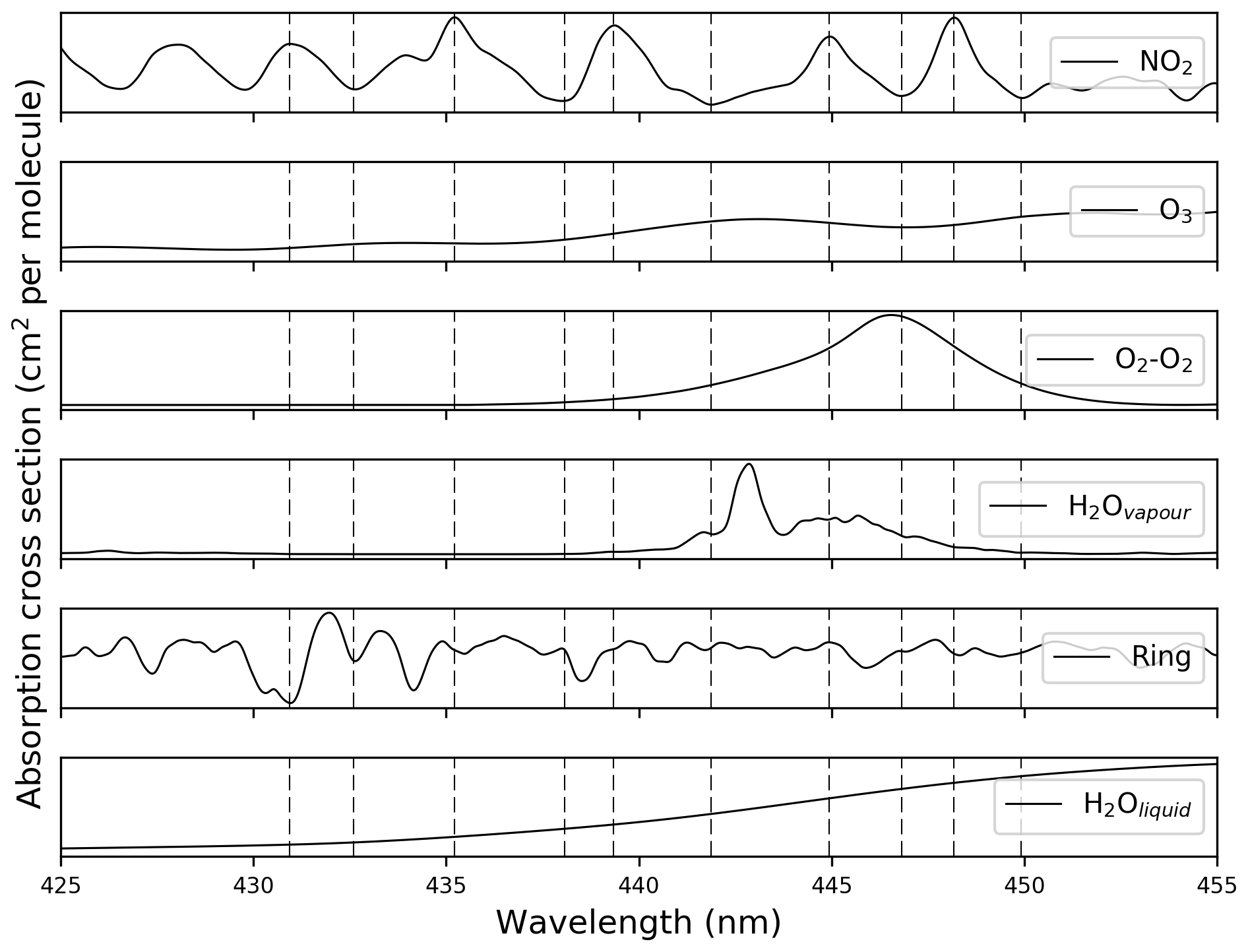
Figure 2 Absorption cross sections of relevant species (solid lines) and position of selected wavelengths (dashed lines) for this study.

2.3 Retrieval

2.3.1 Algorithm description

The retrieval algorithm used in this study is based on elements of DOAS (Platt and Stutz, 2008). There are different implementations of the DOAS technique, mainly the intensity fit (non-linear) and the optical density fit (linear). In DW-DOAS we use the linear approach to obtain the slant column density:

$$\begin{array}{}\text{(2)}& \sum _i{\mathit{\sigma }}_i\left(\mathit{\lambda }\right)\cdot N_{\mathrm{s},i}+P\left(\mathit{\lambda }\right)=-\ln \left({\displaystyle \frac{I\left(\mathit{\lambda }\right)}{I_{\mathrm{0}}\left(\mathit{\lambda }\right)}}\right),\end{array}$$

where σ_i is the absorption cross section of the i species fitted, including the Ring spectrum as a pseudo-absorber (Chance and Spurr, 1997); N_s, i denotes the slant column densities; P(λ) is a low-order polynomial; I(λ) is the Earth radiance; and I₀(λ) is the solar irradiance. Since this equation needs to be solved for each wavelength, the resulting problem is a system of equations. This can be represented with the following linear expression:

$$\begin{array}{}\text{(3)}& {\displaystyle }\mathbf{A}\cdot \mathit{x}=\mathit{B}\text{(4)}& {\displaystyle }\begin{array}{r}\left[\begin{array}{cccccc}{\mathit{\sigma }}_{{\mathrm{NO}}_{\mathrm{2}}}\left({\mathit{\lambda }}_{\mathrm{1}}\right)& {\mathit{\sigma }}_{{\mathrm{O}}_{\mathrm{3}}}\left({\mathit{\lambda }}_{\mathrm{1}}\right)& \mathrm{\cdots }& \mathrm{1}& {\mathit{\lambda }}_{\mathrm{1}}& {\mathit{\lambda }}_{\mathrm{1}}^{\mathrm{2}}\\ {\mathit{\sigma }}_{{\mathrm{NO}}_{\mathrm{2}}}\left({\mathit{\lambda }}_{\mathrm{2}}\right)& {\mathit{\sigma }}_{{\mathrm{O}}_{\mathrm{3}}}\left({\mathit{\lambda }}_{\mathrm{2}}\right)& \mathrm{\cdots }& \mathrm{1}& {\mathit{\lambda }}_{\mathrm{2}}& {\mathit{\lambda }}_{\mathrm{2}}^{\mathrm{2}}\\ \mathrm{⋮}& \mathrm{⋮}& \mathrm{\ddots }& \mathrm{⋮}& \mathrm{⋮}& \mathrm{⋮}\\ {\mathit{\sigma }}_{{\mathrm{NO}}_{\mathrm{2}}}\left({\mathit{\lambda }}_{\mathrm{10}}\right)& {\mathit{\sigma }}_{{\mathrm{O}}_{\mathrm{3}}}\left({\mathit{\lambda }}_{\mathrm{10}}\right)& \mathrm{\cdots }& \mathrm{1}& {\mathit{\lambda }}_{\mathrm{10}}& {\mathit{\lambda }}_{\mathrm{10}}^{\mathrm{2}}\end{array}\right]\\ \cdot \left[\begin{array}{c}{N}_{\mathrm{s},{\mathrm{NO}}_{\mathrm{2}}}\\ N_{\mathrm{s},{\mathrm{O}}_{\mathrm{3}}}\\ \mathrm{⋮}\\ c\\ b\\ a\end{array}\right]=\left[\begin{array}{c}-\ln \left(\frac{I\left({\mathit{\lambda }}_{\mathrm{1}}\right)}{I_{\mathrm{0}}\left({\mathit{\lambda }}_{\mathrm{1}}\right)}\right)\\ -\ln \left(\frac{I\left({\mathit{\lambda }}_{\mathrm{2}}\right)}{I_{\mathrm{0}}\left({\mathit{\lambda }}_{\mathrm{2}}\right)}\right)\\ \mathrm{⋮}\\ -\ln \left(\frac{I\left({\mathit{\lambda }}_{\mathrm{1}}\mathrm{0}\right)}{I_{\mathrm{0}}\left({\mathit{\lambda }}_{\mathrm{1}}\mathrm{0}\right)}\right)\end{array}\right],\end{array}\end{array}$$

where A is an M×N matrix containing the absorption cross sections and the polynomial basis for each wavelength, x is a column vector of N elements containing the slant column densities of the absorbers (N_s, i) and the polynomial coefficients (a, b, c), and B is a column vector of M elements containing the optical density for each wavelength. In order to solve for x we calculate the pseudo inverse of matrix A, namely A⁻¹, using the singular value decomposition (SVD) numerical method to factorise A:

$$\begin{array}{}\text{(5)}& {\displaystyle }& {\displaystyle }\mathbf{A}=\mathbf{U}\cdot \mathbf{W}\cdot {\mathbf{V}}^T,\text{(6)}& {\displaystyle }& {\displaystyle }{\mathbf{A}}^{-\mathrm{1}}=\mathbf{V}\cdot {\mathbf{W}}^{-\mathrm{1}}\cdot {\mathbf{U}}^T,\end{array}$$

where U is an M×N column-orthogonal matrix, W is an M×N diagonal matrix with non-negative real numbers in the diagonal (singular values), and V is an N×N orthogonal matrix.

Although this approach is similar to a traditional DOAS retrieval, there are some differences arising from having only a few discrete spectral points. First, the order of the polynomial must not be greater than 2, as fitting higher-order polynomials results in erroneously low slant column densities. In a way, this limits one of the key advantages of DOAS, that is, the ability to remove the broadband part of the reflectance. However, this can be overcome by having a fitting window narrow enough that the broadband component can be approximated by a second-order polynomial, which is one of the criteria used in this work for wavelength selection (see Sect. 2.2.2). The concept of “fitting window” in the context of DW-DOAS should be interpreted as a spectral range that contains the discrete wavelengths rather than in a literal sense as is the case for hyperspectral DOAS retrievals.

(Boersma et al., 2018)(van Geffen et al., 2020, 2019)

Table 1 NO₂ SCD retrieval details for OMI and TROPOMI reference products and DW-DOAS.

van Geffen et al. (2015)Boersma et al. (2018)van Geffen et al. (2015)

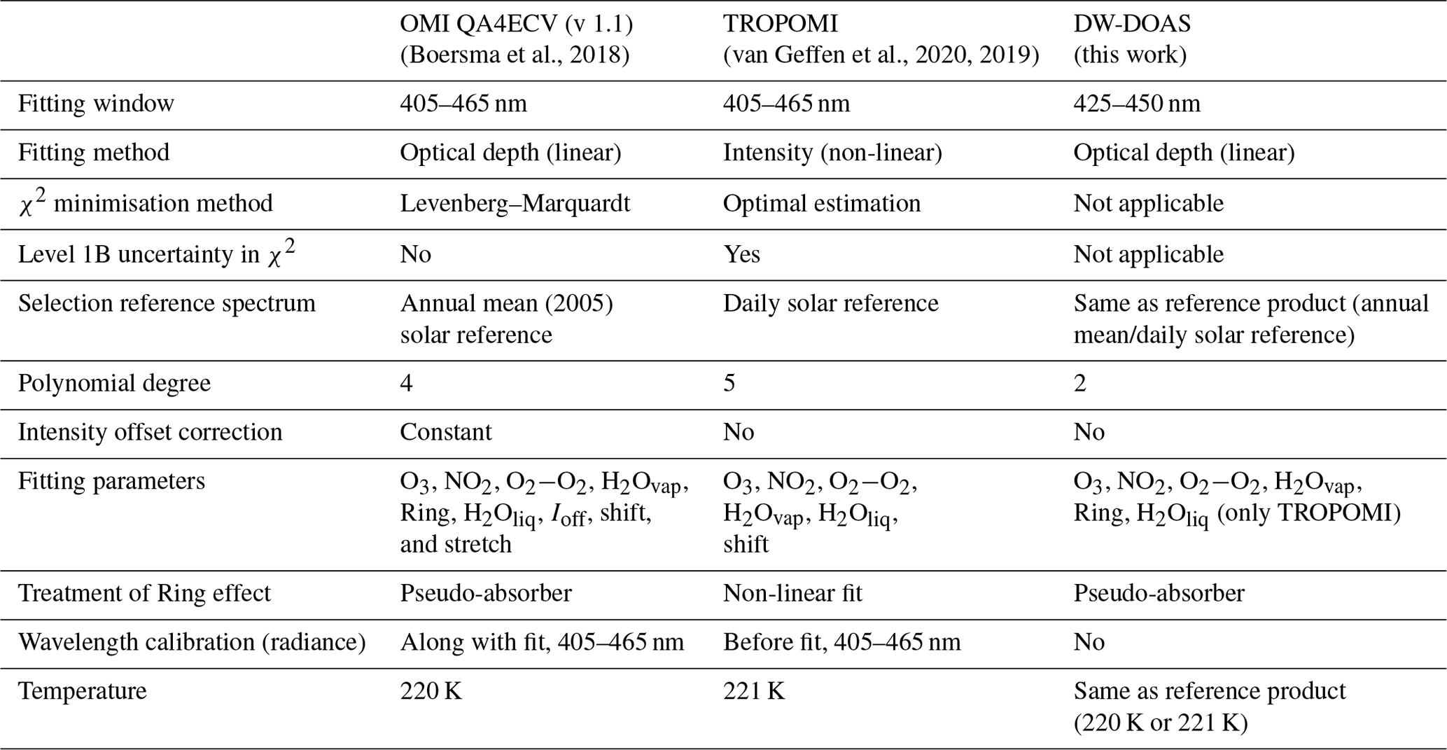
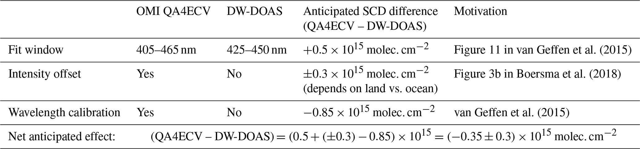
Table 2 Anticipated SCD differences between QA4ECV and DW-DOAS due to retrieval implementation differences, based on the literature.

Another consequence of discretising the spectra is that it is no longer possible to perform a wavelength calibration using the Fraunhofer lines of the solar reference spectrum. Therefore, no wavelength calibration is done as part of the retrieval. The implications of this limitation for a future operational instrument are discussed in Sect. 3.5.

The last difference between discrete and traditional DOAS is related to the ability to perform a “shift and squeeze” to correct for small spectral misalignments. In traditional DOAS two additional non-linear coefficients can be fitted to correct the spectra in this manner. This cannot be done in the context of a discrete-wavelength retrieval owing to the lack of spectral information available, so such parameters are not fitted.

Table 1 shows a comparison between our discrete-wavelength retrieval and the algorithms used for TROPOMI and OMI QA4ECV.

2.3.2 Retrieval uncertainty

The retrieval uncertainty is estimated using a method commonly employed as an independent evaluation of DOAS SCD uncertainty estimations (e.g. Zara et al., 2018; Boersma et al., 2007). The method calculates the uncertainty as the spatial variability of the SCD over a remote area in the Pacific Ocean, which is considered to have background NO₂ concentrations. The assumption is that the variation in the NO₂ SCDs is caused solely by the retrieval uncertainty; therefore, this can be calculated as the standard deviation of spatial spread of SCDs. The area selected corresponds to latitudes between 60^∘ S and 60^∘ N, and longitudes between 150 and 180^∘ W. To account for light path differences the area is divided into 2^∘ × 2^∘ boxes so that the pixels in each box can be assumed to have similar path lengths. The geometric air mass factor (AMF) is used as an indicator of the path length for each pixel; a good description of AMFs can be found in Palmer et al. (2001). Boxes with high geometric AMF variability (>5 %) are discarded. The relative AMF variability is calculated using the expression defined in Zara et al. (2018):

$$\begin{array}{}\text{(7)}& {\text{AMF}}_{\text{var}}={\displaystyle \frac{\sqrt{(\stackrel{\mathrm{‾}}{M_i^{\mathrm{2}}}-{\stackrel{\mathrm{‾}}{M_i}}^{\mathrm{2}})}}{M_i}},\end{array}$$

where M_i is the geometric AMF of each pixel (i) within one box, calculated as a function of the solar zenith angle (θ_s) and the satellite viewing angle (θ_v):

$$\begin{array}{}\text{(8)}& M_i=\sec {\mathit{\theta }}_{\mathrm{s},i}+\sec {\mathit{\theta }}_{\mathrm{v},i}.\end{array}$$

Then we calculate the deviation of each pixel from its box SCD mean and fit a Gaussian to the results, from which we obtain the standard deviation corresponding to the SCD uncertainty.

3 Results and discussion

3.1 OMI NO₂ SCD comparison

As an initial exercise, the NO₂ SCD results from our DW-DOAS retrieval of selected single orbits from January 2005 are compared with the corresponding OMI QA4ECV NO₂ product. Figure 3 shows the results from both retrievals and the relative differences between them. The three orbits selected have a mixture of heavily polluted and clean areas with respect to NO₂. In all three swaths the datasets are highly correlated, with DW-DOAS generally producing lower-NO₂ SCDs (∼5 %). The largest differences are found around the centre of each swath, which coincides with the areas with the lowest SCDs in the QA4ECV dataset. These areas also are around the Equator, where the geometric light paths are shortest. Furthermore, the middle of the swath is where ground pixel sizes are smallest. DW-DOAS is more susceptible to albedo effects than traditional DOAS, so the higher differences might be related to the sub-pixel variability of the albedo. Smaller pixels have lower variability and this might mean that some stronger spectral features might be present that cause higher errors.

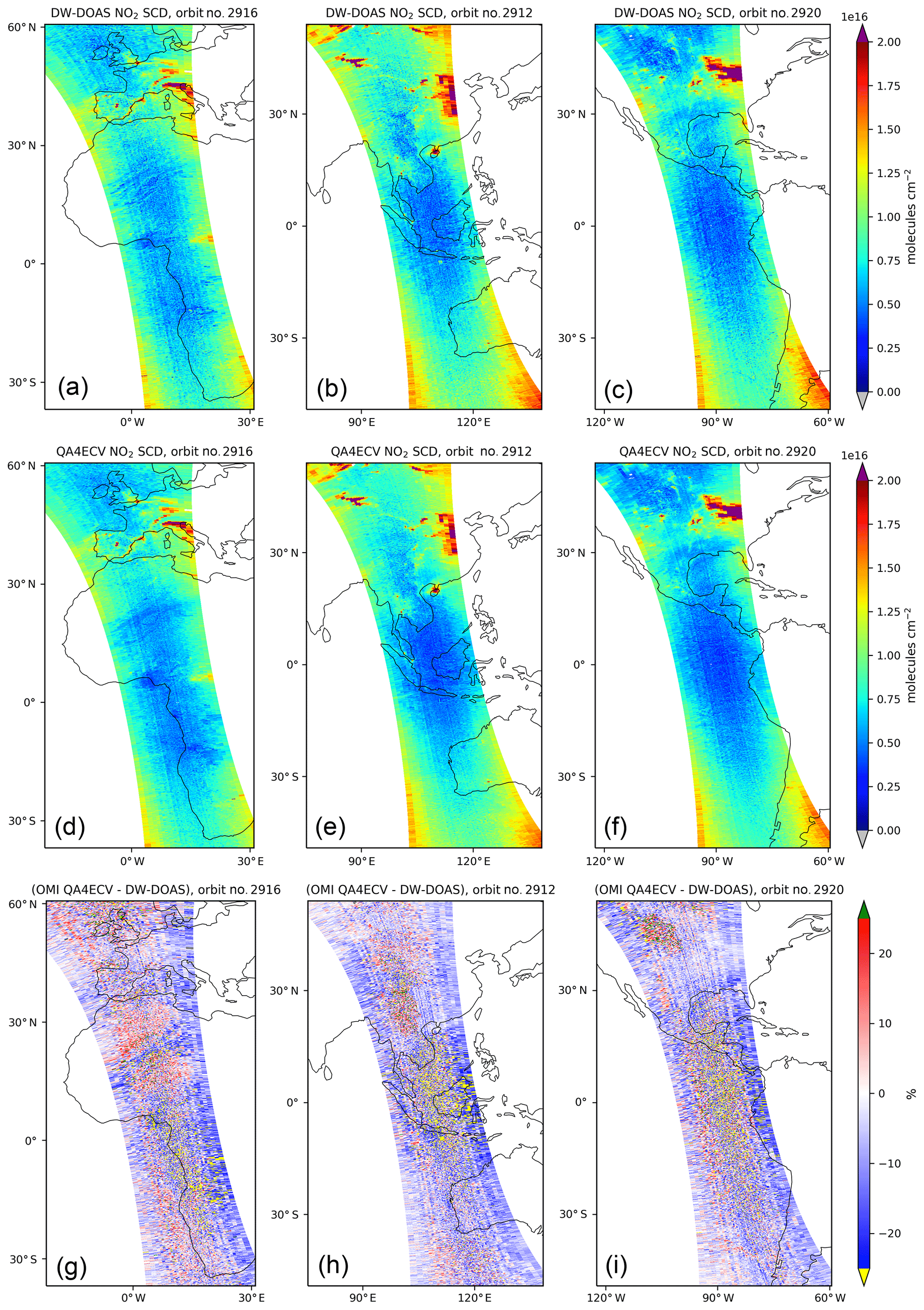
Figure 3 (a, b, c) NO₂ SCDs retrieved by DW-DOAS for selected orbits of 31 January 2005 in all-sky conditions, (d, e, f) corresponding QA4ECV NO₂ SCDs, and (g, h, i) the relative differences between them calculated as (QA4ECV – DW-DOAS) ∕ QA4ECV and expressed in percentage.

It is visually apparent from Fig. 3 that DW-DOAS results are slightly noisier than those retrieved by QA4ECV, particularly over unpolluted areas. This is expected given the limited spectral information available for the retrieval and indicates a lower sensitivity to NO₂ of DW-DOAS compared to hyperspectral retrievals. This difference in noisiness is quantified in the statistical uncertainty estimation (Sect. 3.3).

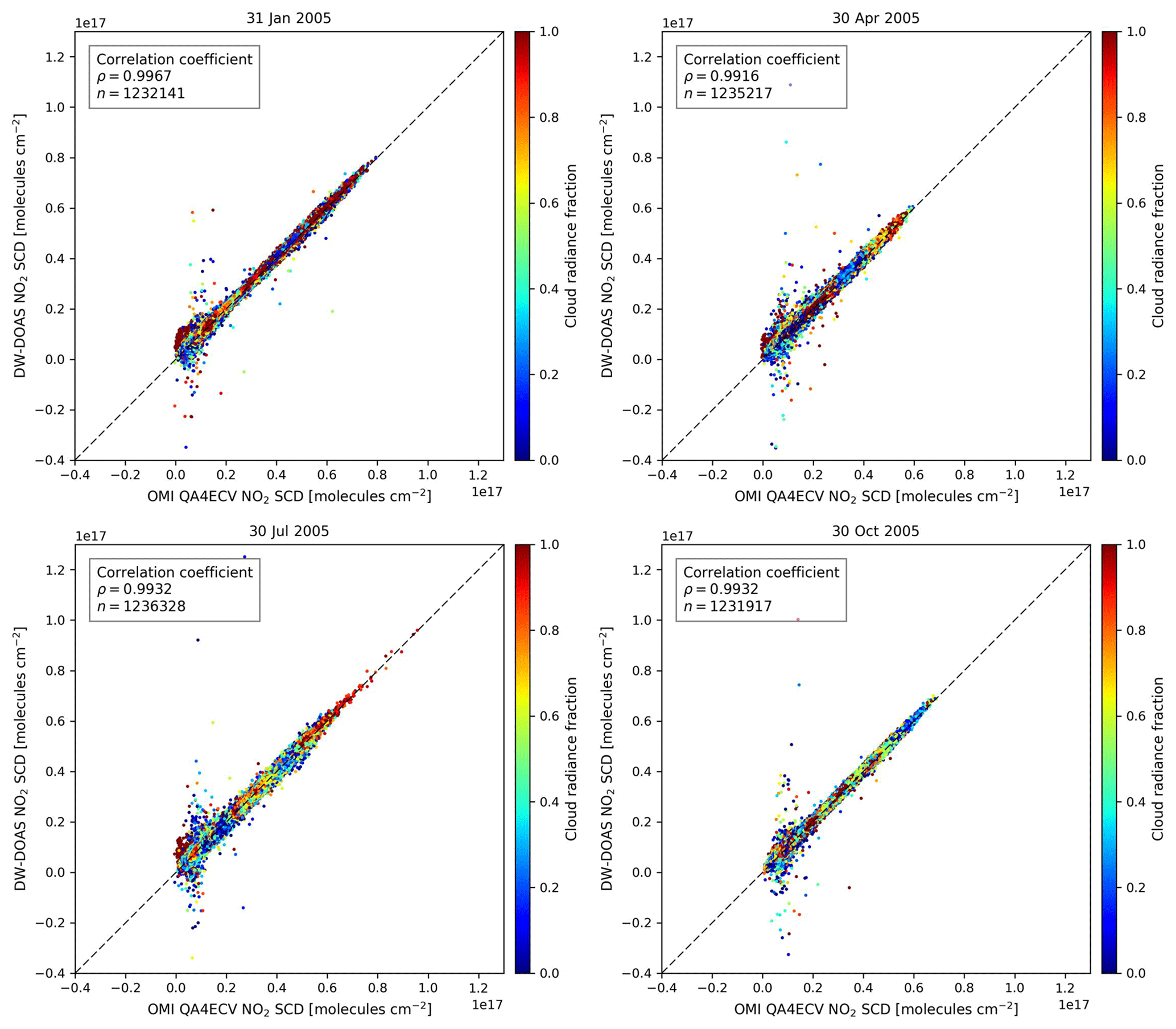
The differences between DW-DOAS and QA4ECV SCDs are normally distributed, as shown in the histograms in Fig. 4. However, the negative biases indicate systematic differences between datasets, which are likely due to differences in retrieval implementation and settings. These biases are within the anticipated values from relevant sensitivity studies from the literature, which are summarised in Table 1. The main differences stem from the absence of wavelength calibration in the case of DW-DOAS, the inclusion of an intensity offset in the fit in the case of QA4ECV, and the differences in the fitting window. Different spectral regions may contain spectral signatures that are not accounted for in the retrieval, which can cause biases when different fitting windows are used (e.g. van Geffen et al., 2015). Also in Fig. 4 are the correlation plots for all the selected swaths. These corroborate the good agreement between datasets that is evident in Fig. 3, with r>0.99 in all cases.

Figure 4 (a, b, c) Distribution of absolute differences between the NO₂ SCDs retrieved by DW-DOAS and QA4ECV for the orbits in Fig. 3, calculated as (QA4ECV – DW-DOAS), and (d, e, f) corresponding correlation plot.

In order to check for any geographical and seasonal variabilities in the results we processed all single orbits from 4 d in January, April, July, and October of 2005. The results can be seen in Fig. 5, which shows the DW-DOAS retrieval results (scaled with the geometric AMF for clarity) and the relative differences with the QA4ECV product. Maps of the absolute differences can be found in Appendix A. Similar patterns to those seen in Fig. 3 for individual orbits are also seen in the global maps of relative differences. The largest differences are seen mainly around the Equator and they are highest in the April data. However, these features seem to be a result of using relative differences with small values and are not present to the same extent in the maps of absolute differences (Fig. A1). Some of the differences observed over the ocean could be attributed to the intensity offset correction that is included in the QA4ECV product. The physical meaning of this term is not well understood, but it is included in the retrieval to account for spectral signatures caused by vibrational Raman scattering on water molecules within the ocean and incomplete Ring corrections, and to prevent O₃ misfits (Boersma et al., 2018).

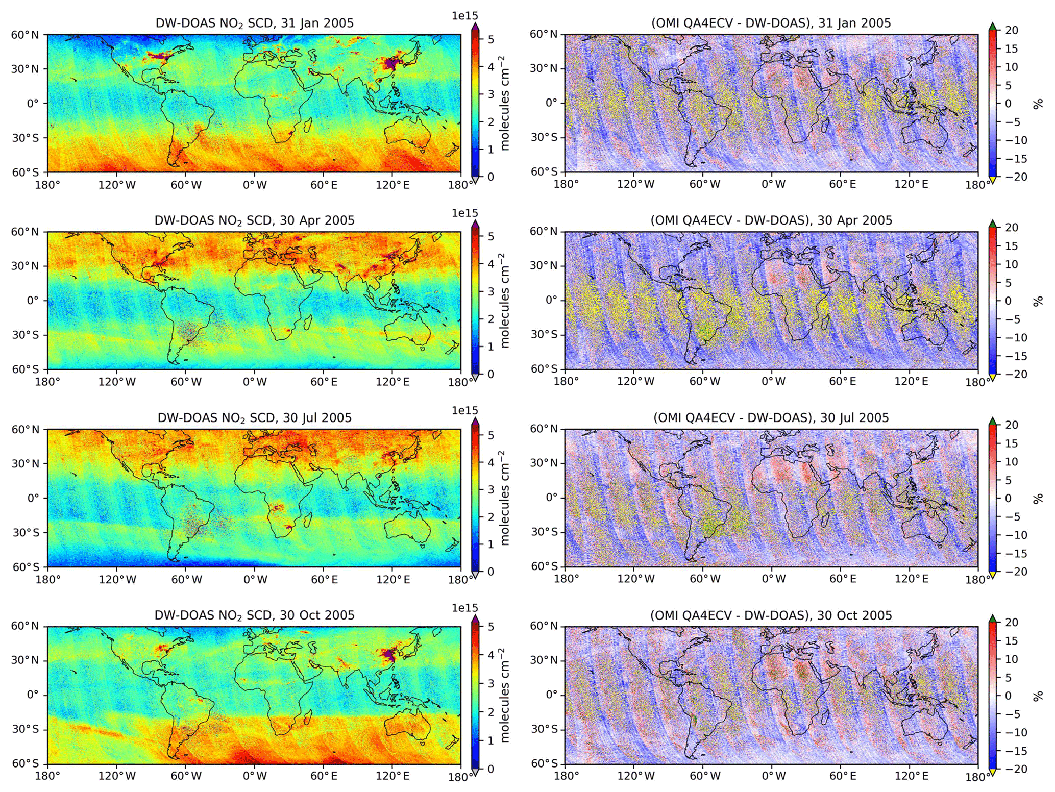
Figure 5 (left) Global DW-DOAS NO₂ SCDs scaled with geometric AMFs (for clearer data visualisation) for all single orbits of 1 d in January, April, July, and October of 2005, and (right) the relative differences with QA4ECV calculated as (QA4ECV – DW-DOAS) ∕ QA4ECV and expressed in percentage. The latitudes are limited to [60^∘ S, 80^∘ N]. Data from all-sky conditions have been used.

Some of the lowest differences are found in large plumes of NO₂, for example, in North America and China in the January map. Two other interesting features stand out from the global maps. Firstly, DW-DOAS seems to consistently underestimate the SCDs over the Sahara desert, which is likely due to the spectral signature of sand. It could be argued that it is the high albedo of the desert causing higher errors, but this only seems to happen significantly over that area. The second feature is found in South America around 30^∘ S, where there is an area of higher differences between retrievals. This is also apparent on the SCD maps, and seems to coincide with the region affected by the South Atlantic Anomaly (SAA), which is known to affect DOAS retrievals (e.g. Richter et al., 2011). The OMI QA4ECV product includes a spike correction that significantly reduces the scatter in the area affected by the SAA, which might explain the differences.

Figure 6 shows the correlation plots for DW-DOAS and QA4ECV using the global NO₂ SCD data from Fig. 5. The agreement between datasets when using global data is reduced owing to spatial features in the differences, as discussed previously. There are more outliers in the data from April and July, and most of them correspond to lower slant column densities and lower cloud radiance fractions. In fact, some of the spatial features that can be seen in Fig. A1 seem to correspond to cloud structures, with lower differences over cloudy pixels. For cloud-free pixels effects such as the surface albedo or lower SNRs, as well as vibrational Raman scattering on water molecules within the ocean (Oldeman, 2018), might be contributing to the higher differences.

Figure 6 Correlation plots of DW-DOAS and QA4ECV global NO₂ SCD data used in Fig. 5. Pixels in the region affected by the SAA (approximated by a rectangle of latitudes [6^∘ S, 40^∘ S] and longitudes [70^∘ W, 16^∘ W]) have been filtered out.

3.2 TROPOMI NO₂ SCD comparison

To extend the study we performed a similar analysis to that done for OMI, described in Sect. 3.1, using data from the TROPOMI NO₂ operational product. First, the results from DW-DOAS for three selected orbits from 31 January 2019 are compared to the operational product (see Fig. 7). As was the case for OMI, there is a high correlation between the datasets, with DW-DOAS producing SCDs ∼11 % smaller than TROPOMI. The largest differences are located towards the centre of the swath and coincide with the lowest SCDs in the TROPOMI operational product. As with OMI data, the differences are smaller in areas with high SCDs.

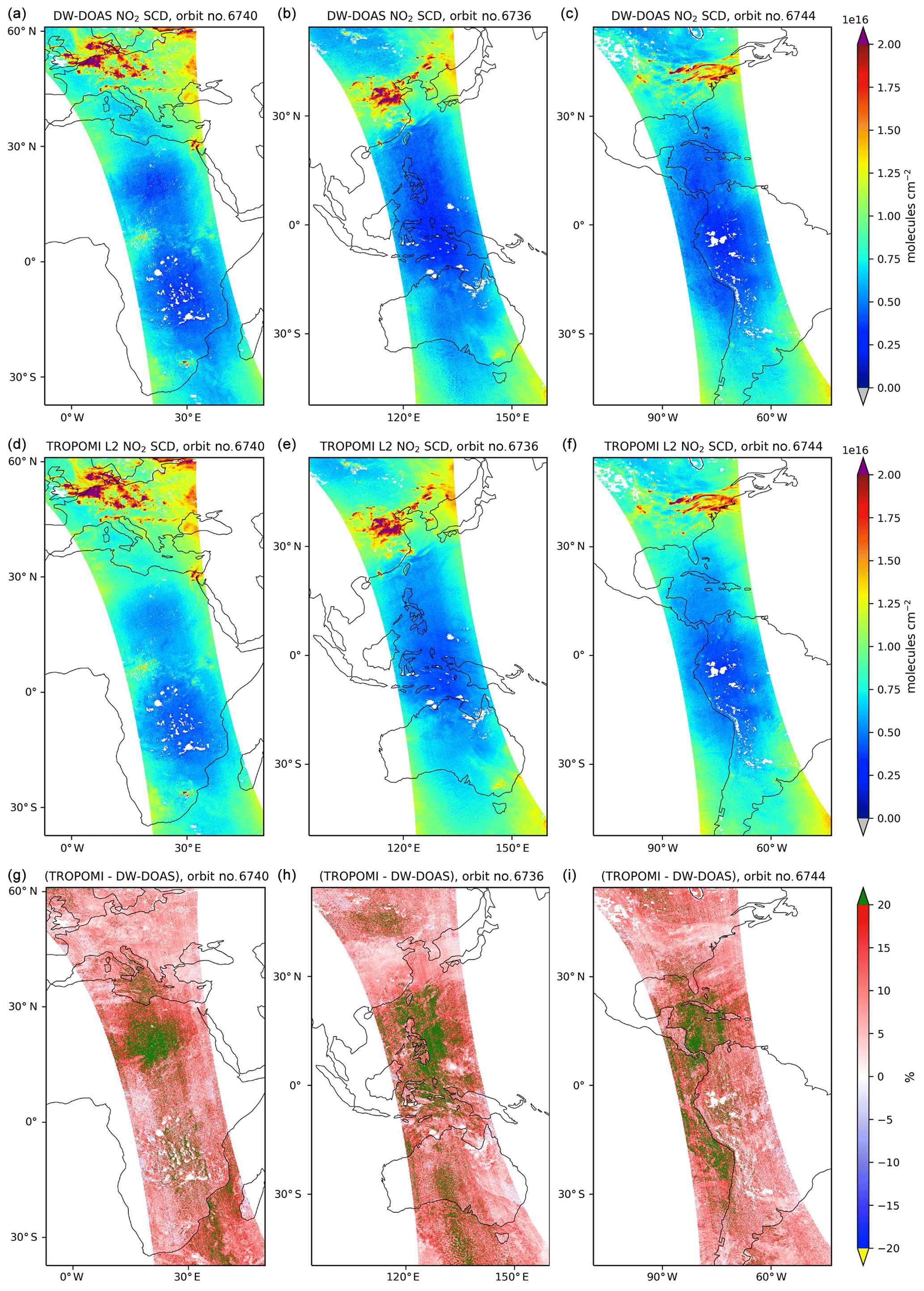
Figure 7 (a, b, c) NO₂ SCDs retrieved by DW-DOAS for selected orbits of 31 January 2019, (d, e, f) corresponding TROPOMI NO₂ SCDs, and (g, h, i) the relative differences between them calculated as (TROPOMI – DW-DOAS)/TROPOMI and expressed in percentage. All the data are screened using the quality assurance flag (qa >0.5) from the TROPOMI NO₂ level 2 dataset, which includes all-sky pixels.

van Geffen et al. (2015)van Geffen et al. (2015)Boersma et al. (2018)

Table 3 Anticipated SCD differences between TROPOMI and DW-DOAS owing to retrieval implementation differences, based on the literature.

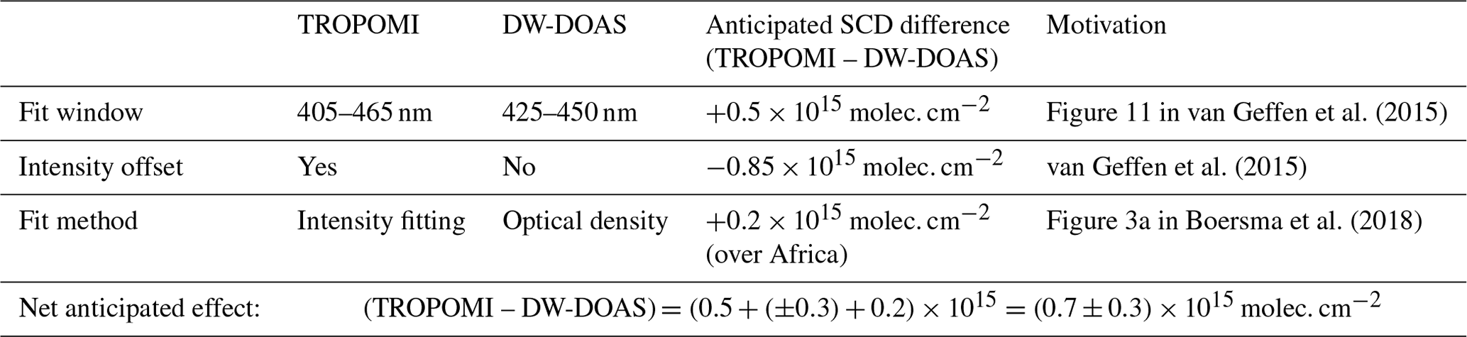
Figure 8 shows the histograms of the differences between retrieval results, and the correlation plots. These are similar to those obtained for OMI and indicate that the differences are normally distributed and that the correlation is better than 0.99. However, in the case of TROPOMI the biases are much larger. Nonetheless, these still fall within the range of expected differences in SCD related to retrieval implementation and settings. Table 3 contains the expected range of SCD differences according to the literature. The main contributions are from differences in fitting window, the inclusion of an intensity offset in the case of TROPOMI, and the different implementation of DOAS (non-linear in the case of TROPOMI, and linear in the case of DW-DOAS). Interestingly, although the biases are higher than in the case of OMI, the standard deviation of the differences between DW-DOAS and TROPOMI is smaller owing to its higher intrinsic SNR.

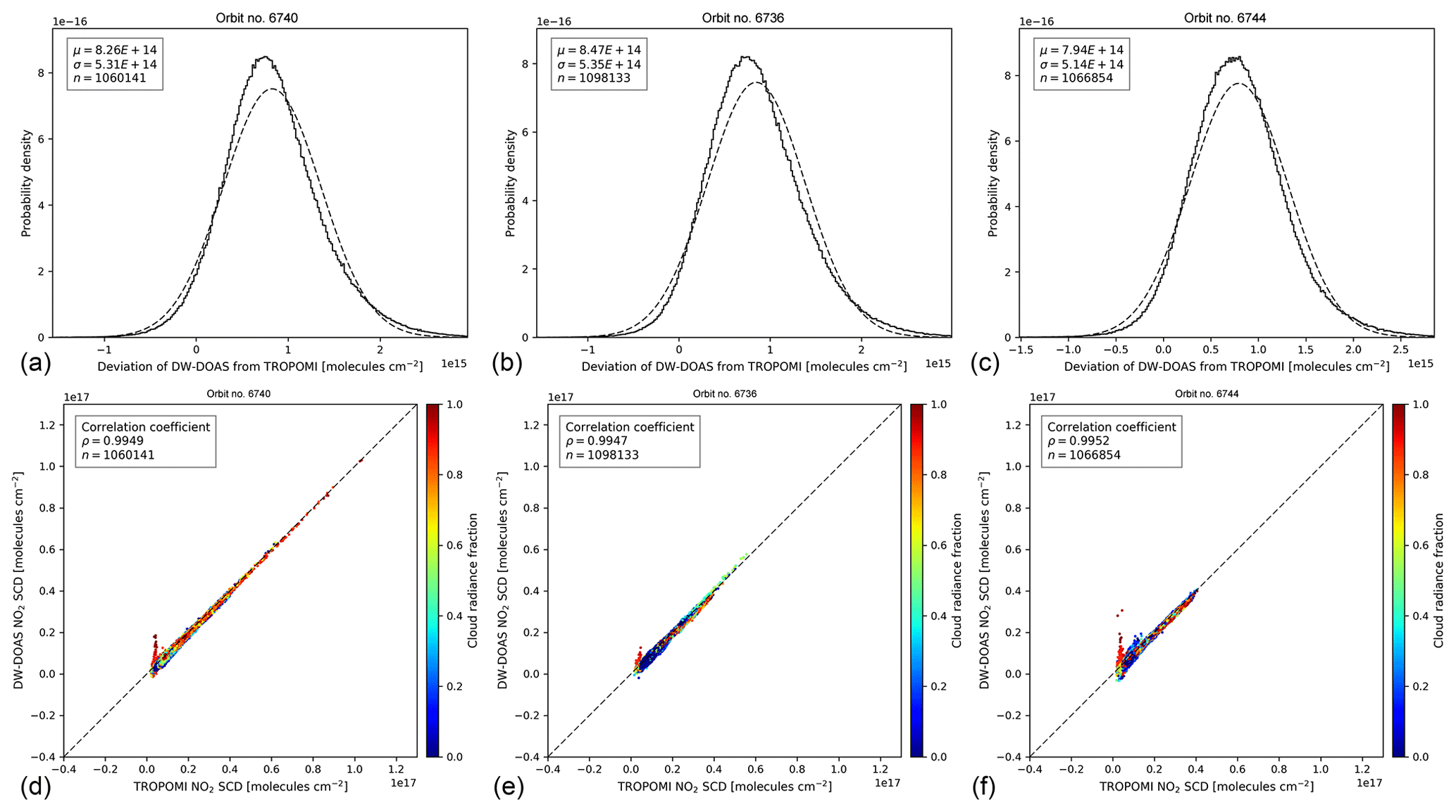
Figure 8 (a, b, c) Distribution of absolute differences between the NO₂ SCDs retrieved by DW-DOAS and TROPOMI for the orbits in Fig. 7, calculated as (TROPOMI – DW-DOAS), and (d, e, f) corresponding correlation plot.

Figure 9 shows the global maps of SCDs retrieved by DW-DOAS and their relative differences with the TROPOMI operational product. Maps of the absolute differences can be found in Appendix A. The patterns in the single orbits are also seen throughout the global data. The largest relative differences are generally found in central across-track pixels and are smaller at the edges of the swaths. While for OMI these were found around the Equator, for TROPOMI they are spread further along the swaths, and are more pronounced over water. As it was the case with OMI, large relative differences are not as strong on the maps of absolute differences (Fig. A1) and they are thought to be partly the result of small SCD values. Interestingly, most of the areas with the largest differences coincide with high liquid water SCDs from the TROPOMI NO₂ Level 2 operational product (retrieved as part of the DOAS fit; not shown here). It is not completely clear what causes these spatial patterns, but surface albedo, cloudiness, smaller pixel sizes, and viewing geometry might play a role. Over land the differences are generally lower, with the exception of the Sahara desert. Unlike for OMI, for TROPOMI the effect of the SAA is not as obvious from the SCD maps, but it can be seen to a lesser extent in the maps of differences.

Figure 9 (left) Global DW-DOAS NO₂ SCDs scaled with geometric AMFs (for clearer data visualisation) for all single orbits of 1 d in January of 2019, and April, July, and October of 2018, and (right) the relative differences with TROPOMI calculated as (TROPOMI – DW-DOAS)/TROPOMI and expressed in percentage. The latitudes are limited to [60^∘ S, 80^∘ N]. All the data are screened using the QA flag (QA >0.5) from the TROPOMI NO₂ level 2 dataset, which includes all-sky pixels.

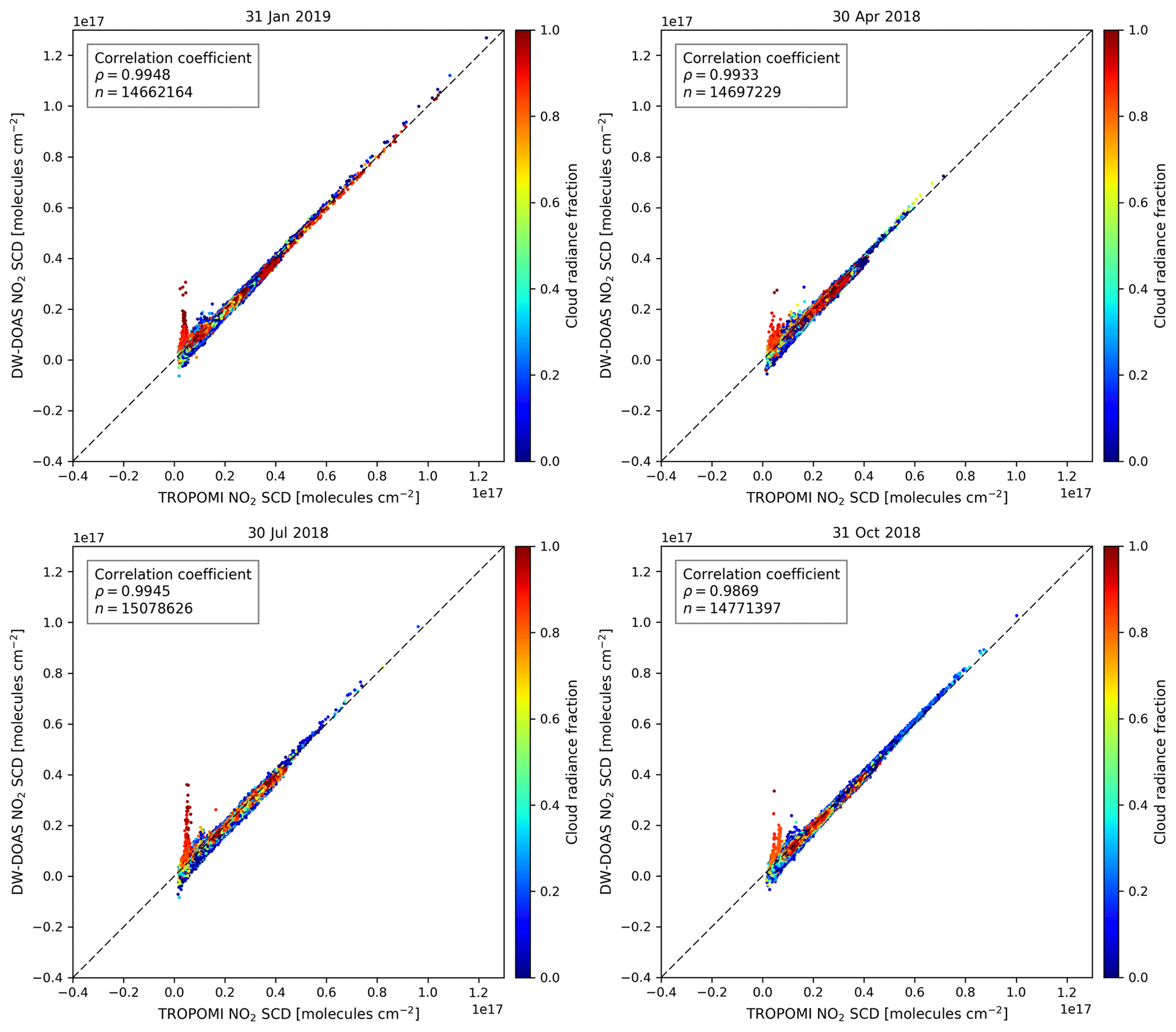
The global correlation plots in Fig. 10 show similar correlation coefficients as those seen for OMI. However, once again the increased SNR is reflected in the standard deviation of the SCD differences, particularly for lower values, where it is markedly smaller than that obtained for OMI. There are fewer outliers and, unlike for OMI, they mostly correspond to pixels with high cloud radiance fraction. The dependence on cloud radiance fraction for both instruments cannot be directly compared, because the OMI and TROPOMI observations are over a decade apart and so will be subject to very different cloud structures. Additionally, TROPOMI has a smaller pixel size and so will experience very different cloud radiance fractions to OMI (Krijger et al., 2007). Finally, there may also be inherent differences between the cloud top heights observed by both instruments based on the different retrieval algorithms they employ; OMI retrieves this parameter using the O₂−O₂ absorption feature at 477 nm (Veefkind et al., 2016), while TROPOMI makes use of the O₂ A-band in its operational retrieval (van Geffen et al., 2019). In addition, the QA4ECV product for OMI includes an intensity offset correction, which is not included in the TROPOMI product, and that may explain some of the differences over the ocean (Oldeman, 2018).

Figure 10 Correlation plots of DW-DOAS and TROPOMI global NO₂ SCD data used in Fig. 9. Pixels in the region affected by the SAA (approximated by a rectangle of latitudes [6^∘ S, 40^∘ S] and longitudes [70^∘ W, 16^∘ W]) have been filtered out.

3.3 SCD uncertainty estimation

We apply the method described in Sect. 2.3.2 to calculate the NO₂ SCD statistical uncertainty for DW-DOAS for OMI and TROPOMI, including all the boxes in the region of interest for all four seasons. In order to validate our estimates, we also apply the method to the reference datasets, namely the OMI QA4ECV and TROPOMI operational products, and compare the results. The calculations only include boxes with low geometric AMF variability (<5 %). An example of the distribution of the deviation of the SCDs from their respective box mean for the January datasets is shown in Fig. 11, and Table 4 contains the average results for all seasons. In all cases DW-DOAS gives higher uncertainty than the reference level 2 datasets, with this difference being more pronounced for OMI data. TROPOMI histograms have a better Gaussian fit, partly due to the higher quality of the data, but largely because its higher spatial resolution means there are more pixels for the same area used in the calculation, i.e. a larger sample size.

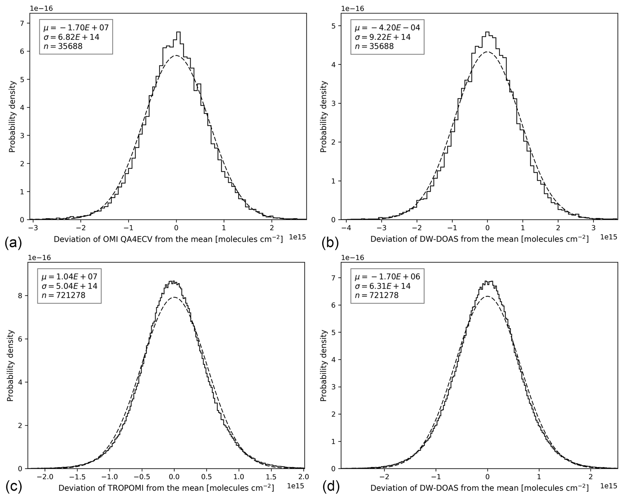
Figure 11 Histogram of the deviation of the NO₂ SCDs from the box mean for OMI (a, b) and TROPOMI (c, d), for DW-DOAS (b, d) and the corresponding reference products (a, c). OMI data have not been screened for clouds; TROPOMI data have been screened using the quality assurance value (qa >0.5) from the level 2 NO₂ product. The data shown are from January 2005 (OMI) and January 2019 (TROPOMI).

We also evaluate the sensitivity of DW-DOAS to striping, which is caused by the inhomogeneous illumination of the entrance slit of the instrument (Dobber et al., 2008). This issue is more pronounced in OMI, and it is usually corrected for after the DOAS retrieval. Figure 12 shows the deviation from the mean SCD scaled with the geometric AMF as a function of across-track pixel number for one orbit over a clean area of the Pacific Ocean. The magnitudes of the peaks and troughs indicate that DW-DOAS has a higher sensitivity to striping compared to OMI QA4ECV, but it is less of an issue for TROPOMI because of the higher quality of the data.

Table 4 Comparison of mean SCD statistical uncertainties for OMI QA4ECV, TROPOMI, and DW-DOAS, calculated from SCDs from a remote area in the Pacific Ocean within latitudes [60^∘ S, 60^∘ N] and longitudes [180^∘ W, 150^∘ W].

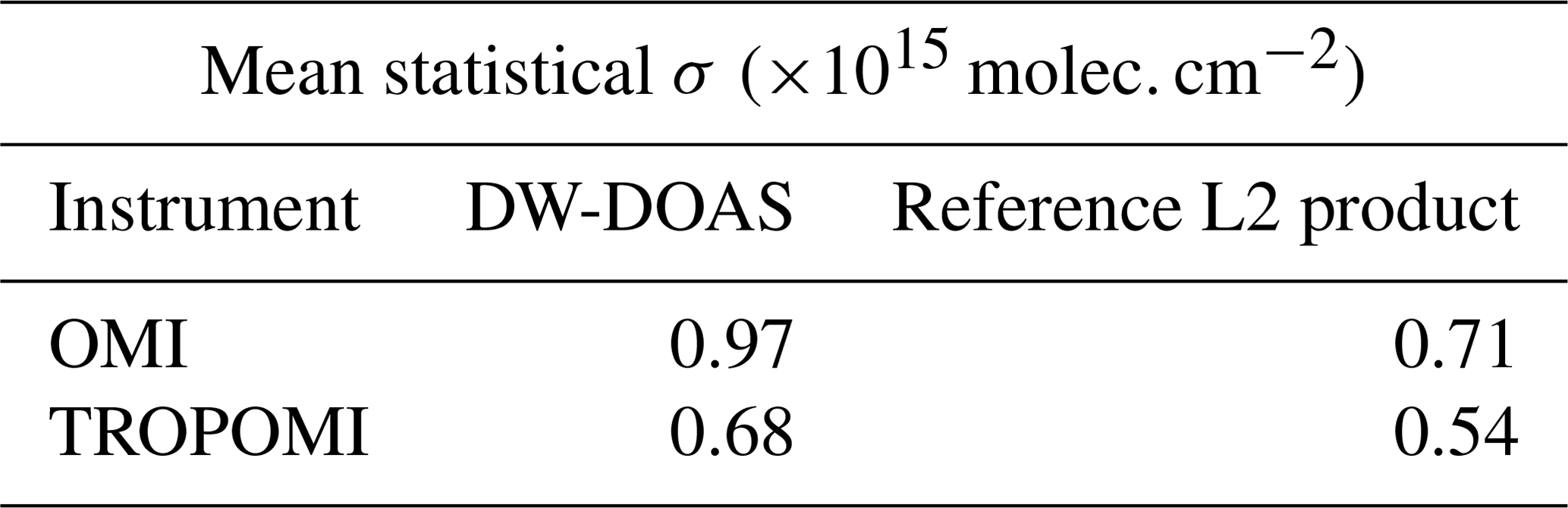
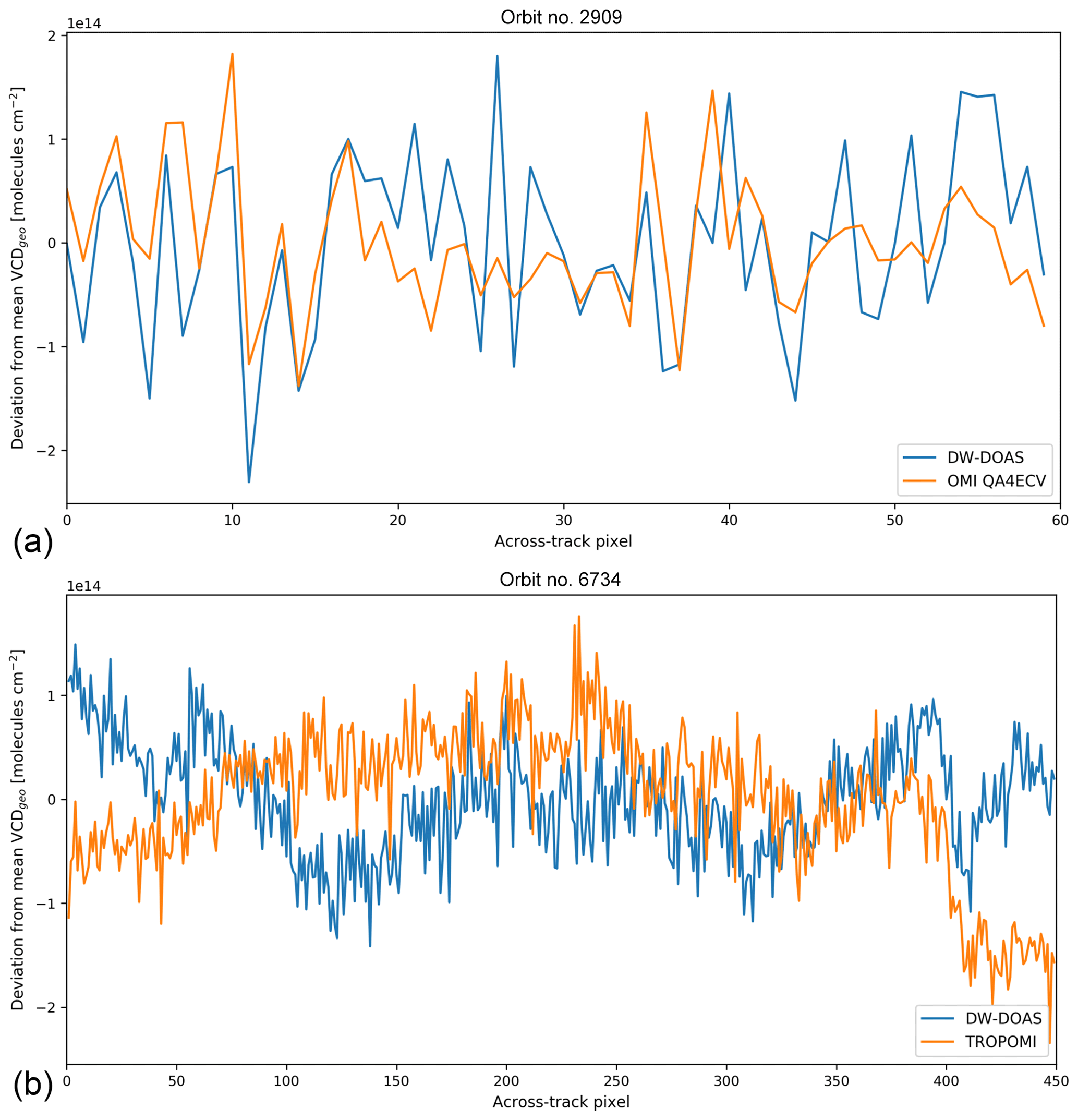
Figure 12 Striping sensitivity of DW-DOAS and the corresponding reference product for (a) OMI and (b) TROPOMI data for one orbit over the Pacific Ocean in the latitude range 30^∘ S–5^∘ N.

3.4 Method limitations

Some of the challenges of using DW-DOAS for NO₂ come from using limited spectral information to retrieve a relatively weak absorber. One limitation is the increased sensitivity to random noise, as seen in the retrieval results and demonstrated by the SCD statistical uncertainty estimations. Another limitation is the higher sensitivity to interfering species, since there is not enough spectral information to completely separate out the gas of interest from the other species. However, the effect of this can be minimised by optimising the wavelength selection.

Furthermore, DW-DOAS has particular limitations that stem from the use of discrete wavelengths in combination with the DOAS retrieval technique. Firstly, one of the basic premises of DOAS is the removal of broadband structures from the reflectance spectra using a polynomial, typically fourth or fifth order. As explained in Sect. 2.3.1, using a polynomial of such a high degree would cause the retrieval to underestimate the NO₂ SCD, so this is limited to a second-order polynomial. However, sometimes this is not enough to remove complex surface albedo or scattering broadband structures. These residual structures might be the underlying cause behind some of the higher SCD differences between DW-DOAS and the OMI and TROPOMI reference products, and these structures can be minimised by selecting channels that are close together so that they can be approximated by a second-order polynomial.

Finally, wavelength calibration using a high-resolution solar reference is an important step in DOAS retrievals because even a small wavelength shift can cause retrieval errors. With discrete-wavelength data it is not possible to use the Fraunhofer lines of the solar spectrum for the wavelength calibration. While this is a shortcoming, it is anticipated that small wavelength shifts do not have as big an impact as they do for hyperspectral DOAS precisely because the spectral channels are sparse and not contiguous, and because the filters are wider.

3.5 Considerations for future instruments

The DW-DOAS results we have presented are promising and the method has the potential to be applied to new satellite instrument designs. However, several aspects need to be considered before it can be implemented in an operational instrument:

• Reference spectrum. The DW-DOAS method has only been tested using a solar spectrum as the reference (I₀) for the DOAS fit. However, earthshine radiance spectra could be used instead, as demonstrated by Anand et al. (2015). Using these spectra would simplify the instrument design by removing the need for a solar diffuser and a solar measurement mode; it would cancel out some instrumental effects and reduce the effect of the Ring structures in the retrieval. Moreover, in theory a synthetic solar spectrum could also be used. Nevertheless, all options come with drawbacks, so a sensitivity study would be needed to find the approach that provides the best results.

• Wavelength calibration and filter response function. As discussed in Sect. 3.4, it is not possible to perform a wavelength calibration for DW-DOAS using a solar reference spectrum owing to the lack of spectral information. Thus, a mechanism for in-flight monitoring of the spectral response of the filters would be critical, since these need to be known accurately to convolve the absorption cross sections.

• Cloud retrieval. To use DW-DOAS operationally a cloud retrieval would be needed to identify cloudy pixels. In other retrieval algorithms using visible spectra this is performed using knowledge of the O₂−O₂ slant column, which can be derived from its absorption cross section peak at ∼477 nm (Veefkind et al., 2016). However, it is not possible to retrieve O₂−O₂ with the wavelengths proposed in this work because they are optimised for NO₂. Therefore, further work is needed to find a suitable solution, for example by adding a few channels to detect the aforementioned O₂−O₂ peak.

• AMF calculations. This work has evaluated the performance of the NO₂ SCD retrieval. However, that is only the first of the three steps in an NO₂ tropospheric vertical column retrieval, which is the final product for the typical end user. The other two steps are the stratospheric–tropospheric NO₂ separation (e.g. model assimilation, Boersma et al., 2011) and the conversion of SCDs into vertical column densities (VCDs) using air mass factors (AMFs; Palmer et al., 2001). These two steps are mostly independent from the SCD fit, so in principle no major differences are expected for DW-DOAS. However, further work is needed to test these and ensure that any retrieval-dependent sensitivities are understood before DW-DOAS is implemented in an operational instrument. This is particularly true for very high spatial resolutions, where the surface albedo might be a problem for DW-DOAS owing to the polynomial limitation.

4 Conclusions and further work

We have developed a method, DW-DOAS, to perform NO₂ slant column density retrievals using only 10 discrete spectral channels and the DOAS technique. It has been tested using OMI and TROPOMI datasets and found to produce results that are comparable to the reference level 2 products, with a mean difference of ∼5 % for OMI QA4ECV and ∼11 % for TROPOMI. However, DW-DOAS has higher uncertainties, which are due to a higher sensitivity to noise, and it is more sensitive to striping. While there is a high correlation (r>0.99) of the DW-DOAS results with the reference level 2 products, some spatial variabilities are found. The largest differences are seen over water, in the Sahara desert, and in clear-sky areas with low NO₂ SCDs. In addition, the centre of the swath presents higher differences. The cause of these is not completely clear, but low NO₂ concentrations, cloudiness, and short light paths might play a role.

The main advantage of the DW-DOAS method over existing DOAS retrievals is the need for comparatively little spectral information, which makes the retrieval faster and would allow potential instrument designs with high spatial resolution. Limitations of the method include higher sensitivity to broadband structures such as surface albedo; higher sensitivity to noise, which means a higher SNR is required; inability to perform a wavelength calibration using a high-resolution solar reference; and the ability to retrieve only NO₂, although with further work it might be possible to retrieve other species by adding a small number of channels.

Despite the shortcomings, our results show that the DW-DOAS method has potential. It could be used in future satellite instruments to allow simpler designs, for example, by having individual optical channels, each with an optical filter and a detector, instead of the traditional spectrometer with a diffraction grating and mirrors. Two of the main challenges of this kind of approach are the co-registration and cross-calibration of the individual channels. In addition, we anticipate that the requirements of spectral accuracy and stability would be more restrictive, particularly given the narrow bands, the limited number of channels, and the more challenging in-flight calibration (it is not possible to use the Fraunhofer lines). However, a comprehensive sensitivity analysis is required to further assess the operational feasibility of such an instrument concept and derive performance requirements.

DW-DOAS in combination with a simple, compact instrument design could be used in low-cost constellations for air quality monitoring at high resolution. This type of constellation could be a good complement to existing high-budget hyperspectral instruments such as OMI and TROPOMI, for example, for the detection of small-scale NO₂ hotspots, which could potentially be identified from space and investigated further using in situ instruments. Furthermore, DW-DOAS could potentially be used for faster retrievals (e.g. for near-real-time processing) for hyperspectral data from existing instruments. Processing speed is especially important for higher data volumes expected by future high-resolution instruments.

Next steps for this work shall include optimising the DW-DOAS method, particularly the channel selection, including the selection of optimal centre wavelengths, number of channels, filter widths, and a comprehensive sensitivity study. Moreover, the practicalities of implementing this method on a real instrument need further assessment: wavelength calibration, reference spectrum (I₀) for the DOAS retrieval (earthshine vs. solar spectrum), cloud retrieval, and the next stages of the NO₂ retrieval (tropospheric–stratospheric separation, and AMF calculation).

Appendix A: Absolute differences between DW-DOAS and OMI and TROPOMI

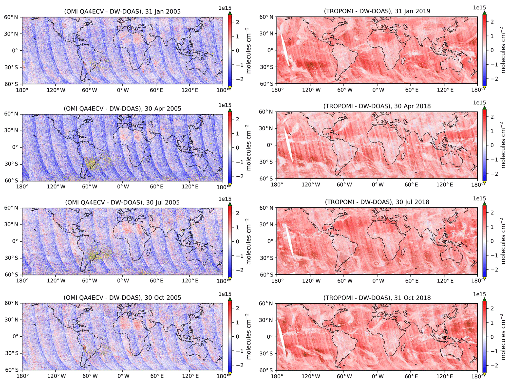
Figure A1 shows the absolute differences between the geometric column densities (i.e. SCDs scaled with the geometric AMFs) as retrieved by DW-DOAS and the OMI/TROPOMI L2 reference products.

Figure A1 Absolute differences between DW-DOAS and (left) OMI QA4ECV and (right) TROPOMI, for the data shown in Figs. 5 and 9. The differences are expressed in terms of the SCD scaled with the geometric AMF. The latitudes are limited to [60^∘ S, 80^∘ N].