the Creative Commons Attribution 4.0 License.
the Creative Commons Attribution 4.0 License.
 | 11 May 2020
A machine-learning-based cloud detection and thermodynamic-phase classification algorithm using passive spectral observations
Steven Platnick
Kerry Meyer
Zhibo Zhang
Yaping Zhou
We trained two Random Forest (RF) machine learning models for cloud mask and cloud thermodynamic-phase detection using spectral observations from Visible Infrared Imaging Radiometer Suite (VIIRS) on board Suomi National Polar-orbiting Partnership (SNPP). Observations from Cloud-Aerosol Lidar with Orthogonal Polarization (CALIOP) were carefully selected to provide reference labels. The two RF models were trained for all-day and daytime-only conditions using a 4-year collocated VIIRS and CALIOP dataset from 2013 to 2016. Due to the orbit difference, the collocated CALIOP and SNPP VIIRS training samples cover a broad-viewing zenith angle range, which is a great benefit to overall model performance. The all-day model uses three VIIRS infrared (IR) bands (8.6, 11, and 12 µm), and the daytime model uses five Near-IR (NIR) and Shortwave-IR (SWIR) bands (0.86, 1.24, 1.38, 1.64, and 2.25 µm) together with the three IR bands to detect clear, liquid water, and ice cloud pixels. Up to seven surface types, i.e., ocean water, forest, cropland, grassland, snow and ice, barren desert, and shrubland, were considered separately to enhance performance for both models. Detection of cloudy pixels and thermodynamic phase with the two RF models was compared against collocated CALIOP products from 2017. It is shown that, when using a conservative screening process that excludes the most challenging cloudy pixels for passive remote sensing, the two RF models have high accuracy rates in comparison to the CALIOP reference for both cloud detection and thermodynamic phase. Other existing SNPP VIIRS and Aqua MODIS cloud mask and phase products are also evaluated, with results showing that the two RF models and the MODIS MYD06 optical property phase product are the top three algorithms with respect to lidar observations during the daytime. During the nighttime, the RF all-day model works best for both cloud detection and phase, particularly for pixels over snow and ice surfaces. The present RF models can be extended to other similar passive instruments if training samples can be collected from CALIOP or other lidars. However, the quality of reference labels and potential sampling issues that may impact model performance would need further attention.
- Article
(6873 KB) - Full-text XML
- BibTeX
- EndNote


Detection and classification (DC) of atmospheric constituents using satellite observations is often a critical initial step in many remote sensing algorithms. For example, a prerequisite for cloud optical and microphysical property retrievals is identifying the presence of clouds, i.e., a clear or cloudy classification (Frey et al., 2008; Heidinger et al., 2012). Additionally, characteristics such as cloud thermodynamic phase are needed, as they can strongly impact the scattering and absorption properties of cloud droplets and particles (Pavolonis et al., 2005; Platnick et al., 2017a). Similarly, current operational aerosol algorithms can only retrieve aerosol optical depth (AOD) for “non-cloudy” pixels since even slight cloud contamination can result in erroneously high retrieved AOD (Remer et al., 2005). Therefore, errors in detecting and classifying atmospheric components can significantly impact downstream retrieval products and scientific analyses.
There are many examples of hand-tuned DC algorithms designed for satellite instruments. For example, the Moderate Resolution Imaging Spectroradiometer (MODIS) has algorithms developed for cloud masking (Frey et al., 2008; Ackerman et al., 2008), cloud thermodynamic phase (Baum et al., 2012; Marchant et al., 2016), aerosol type (Levy et al., 2013; Sayer et al., 2014), and snow coverage over land surfaces (Hall and Riggs, 2016). Decision trees or voting schemes involving multiple thresholds are typically used in these hand-tuned algorithms. The decision tree branches, tests, and thresholds are often determined empirically after a tedious hand-tuning and testing process based on the developer's experience and access to validation datasets. Further, the branches and thresholds are often very sensitive to the specific instrument (e.g., spectral band pass, calibration, noise characteristics, and view and solar geometry sampling). Therefore, an obvious weakness of these hand-tuned methods is that it is challenging and time-consuming to develop algorithms across multiple instruments and to maintain performance for individual instruments that may have noticeable calibration drifts. Meanwhile, a well-designed hand-tuned method may have remarkable performance in a specific region and season yet have significant biases when applied globally and/or annually (Cho et al., 2009; Liu et al., 2010). Additional complexities arise when DC problems become more nonlinear across large spatial and temporal scales, and more variables need to be considered. It is difficult to develop and apply a single or a few decision trees to complicated nonlinear problems that are controlled by a dozen or more variables. As expected, a single decision tree can grow very deep and tends to have a highly irregular structure in order to consider a large number of features (variables) simultaneously, leading to a significant overfitting effect (i.e., an over-constrained training that makes predictions too close to the training dataset but fails to predict future observations reliably). For example, MODIS provides an all-day cloud-phase product based only on infrared (IR) observations (hereafter referred to as IR phase, Baum et al., 2012). Although it can be expected that the tests and thresholds should vary with satellite-viewing geometry (Maddux et al., 2010), full consideration of viewing geometries, together with the variations of many other factors such as surface emission, geolocation, and cloud properties, is very challenging based on manual tuning. As a consequence, it is found that the liquid water and ice cloud fractions from the IR-phase product exhibit noticeable view zenith angle (VZA) dependency (see Fig. 12). This is an undesirable but unavoidable artifact since cloud-phase statistics should be independent of solar and satellite-viewing geometry. Such VZA dependencies may strongly affect similar products from geostationary imagers because of the fixed VZA geolocation mapping. Similar artifacts may also impact aerosol type and retrieval products (Wu et al., 2016).
In contrast to hand-tuned methods, machine-learning (ML)-based DC algorithms are designed to autonomously find information (e.g., patterns of spectral, spatial, and/or time series) in one or more given datasets and learn hidden signatures of different objects. An obvious advantage of ML models is that the training process is efficient and highly flexible. Manually defined thresholds or matching conditions to expected spectral patterns are no longer needed. Recently, ML models have been utilized in a wide variety of cloud- and aerosol-related applications, such as cloud detection (Thampi et al., 2017), cirrus detection and optical property retrievals (Kox et al., 2014; Strandgren et al., 2017), surface-level PM2.5 concentration estimation (Hu et al., 2017), and automatic ship-track detections (Yuan et al., 2019). In this paper, we developed two ML-based DC algorithms for detecting cloud and cloud thermodynamic phase for different local times (i.e., daytime and nighttime) with observations from the Visible Infrared Imaging Radiometer Suite (VIIRS) on board Suomi NPP (SNPP). The ML models are trained with collocated observations from SNPP VIIRS and Cloud-Aerosol Lidar with Orthogonal Polarization (CALIOP), with CALIOP data used as the reference. In Sect. 2, we give a brief discussion of the ML models. Data generated for model training and validation will be introduced in Sect. 3. Details of the model training and evaluation are shown in Sect. 4. Section 5 discusses the advantages and potential limitations of the present ML models. Conclusions are given in Sect. 6.
2.1 Hand-tuned DC methods
All DC algorithms with remote sensing observations are based on the underlying physics of the spectral, spatial, and/or temporal structures of specified objects. In hand-tuned DC algorithms, all the physical rules and structures have to be explicitly defined as various tests and thresholds. For example, the MODIS MOD35/MYD35 cloud mask algorithm uses more than 20 tests with visible or near-infrared (VNIR), shortwave-infrared (SWIR), and infrared (IR) observations (Frey et al., 2008) that are carefully designed to consider numerous scenarios, including different surface types (e.g., ocean, land, desert, snow, etc.) and local times (day or night). Similar algorithms are designed for aerosol type and cloud thermodynamic-phase classifications. As an example, Fig. 1 illustrates spectral patterns of five typical daytime oceanic scenes (pixel types) observed by SNPP VIIRS. The spectral pattern of each of the five scenes, i.e., clear sky, liquid water cloud, ice cloud, dust, and smoke, is averaged by using more than 1000 pixels with the same type. It is clear that the five scenes are different in either reflectance ratios between a given VNIR–SWIR band and the 0.86 µm band or brightness temperature differences (BTD) between two IR window bands (Fig. 1). Consequently, such spectral features are frequently used to differentiate pixel types in DC algorithms. In addition to spectral patterns, simple methods are developed to take spatial information into account . For example, it is found that cloud reflectance usually has larger spatial variability than aerosols (Martins et al., 2002) and clear sky pixels (Platnick et al., 2017a). Therefore, spatial variabilities of VNIR and SWIR reflectance bands are used to differentiate clouds from non-cloudy pixels in the current MODIS clear sky restoral (CSR) algorithm (Platnick et al., 2017a) and Dark Target aerosol retrieval algorithm (Levy et al., 2013).
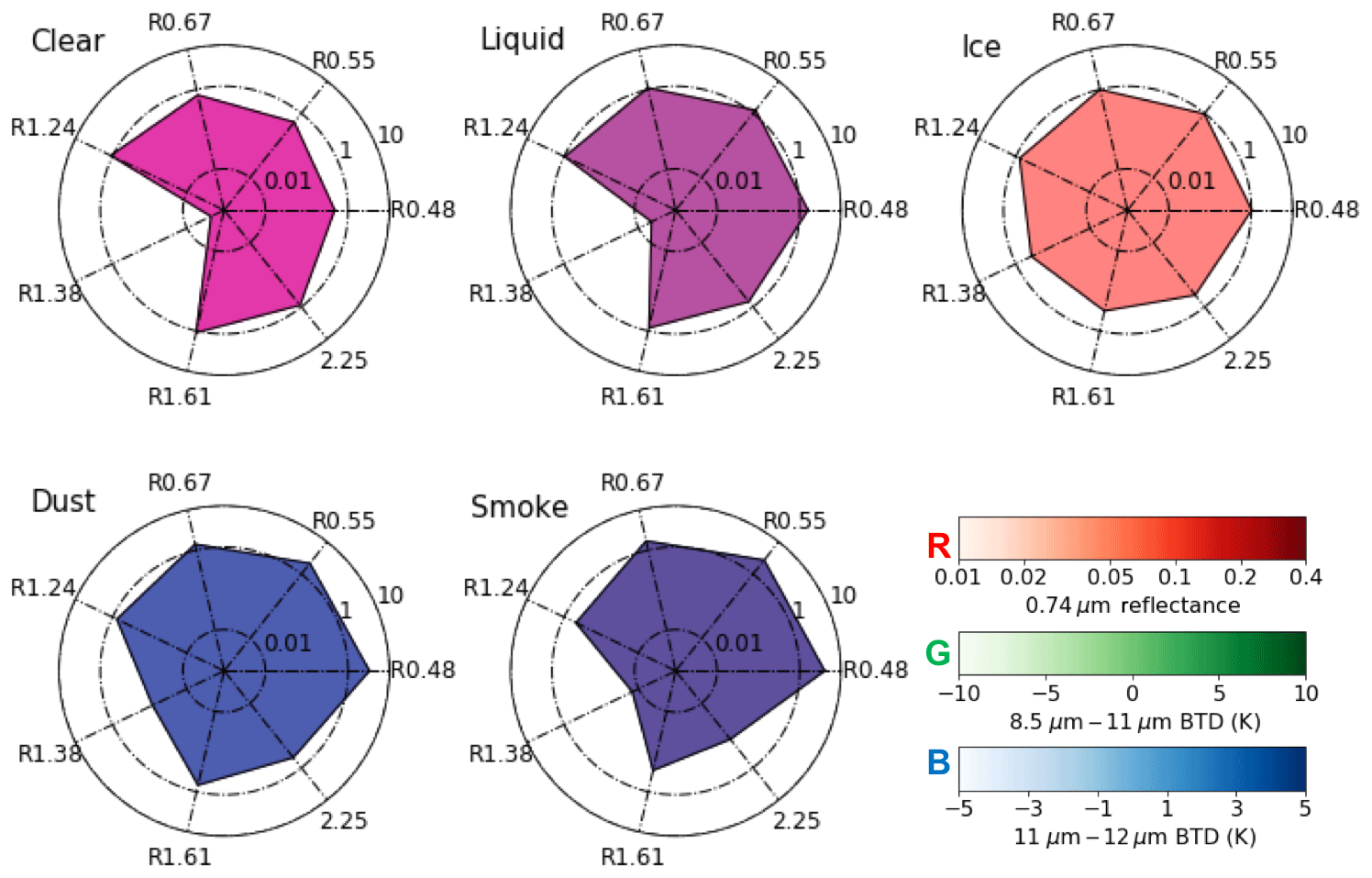
Figure 1Spectral patterns of the five different pixel types (averaged over 1000 pixels for each type). For each plot, an apex indicates reflectance ratio between a given VNIR–SWIR band and the 0.86 µm band, and the spread is filled by false RGB composite (red: 0.74 µm reflectance; green: 8.5–11 µm BTD; blue: 11–12 µm BTD). The spectral patterns are used in the machine learning algorithms.
2.2 Machine learning models
Different from the hand-tuned DC methods, ML algorithms are developed to autonomously learn the hidden spectral, spatial, and temporal patterns of different objects. Consequently, manually defined thresholds or matching conditions to expected patterns are no longer needed. In image recognition applications, numerous ML algorithms (e.g., Joachims, 1998; Breiman, 1999; Dietterich, 2000) were developed in late 1990s for independent pixels using a single or small number of decision trees. Ho (1998) and many other studies have demonstrated that, although these single or small number of decision trees can always provide maximum prediction accuracies in training processes, significant overfitting effects cannot be avoided. Tremendous efforts have been made to overcome the dilemma between maintenance of prediction accuracy and avoiding overfitting. Among these, the Random Forest (RF) and Gradient Boosting (GB) algorithms (Breiman, 1999; Dietterich, 2000; Friedman, 2001) provide a framework of using a large number of decision trees (ensemble) but a subset of features in each tree to achieve optimization in the performance. It has been demonstrated that the ensemble-based algorithms can largely correct mistakes made by individual trees (Ji and Ma, 1997; Tumer and Ghosh, 1996; Latinne et al., 2001) and avoid overfitting (Freund et al., 2001). Currently, the RF and GB algorithms are frequently used in nonlinear classification and regression problems. For example, RF models have been used in several cloud and aerosol remote sensing applications, such as differentiating cloudy from clear footprints for the Clouds and the Earth's Radiation Energy System (CERES) instrument (Thampi et al., 2017), estimating surface-level PM2.5 concentrations (Hu et al., 2017), and detecting low clouds with the Advanced Baseline Imager (ABI) on the Geostationary Operational Environmental Satellites (GOES) (Haynes et al., 2019). In our study, we also choose the RF model based on its proven record in Earth science applications.
In the RF model, a final prediction is made based on majority vote computed from probability (Pi) of each class (ith):
where m is the total number of classes, Ni and Nj are the number of trees that predict the ith and jth classes, and wi and wj are weightings for the ith and jth classes, respectively. If all trees are equally weighted, w for each individual class is equal to 1. The two most important parameters for tuning the RF algorithm are the number of decision trees (NTree) and the maximum tree depth (NDepth). However, an optimal definition of these two parameters is still an open question (Latinne et al., 2001). Larger NTree and NDepth provides more accurate predictions at the cost of significantly increased computational resources. For many cases, larger NDepth may cause overfitting effects (Oshiro et al., 2012; Scornet, 2018). Generally, the two parameters have to be large enough to let the decision trees have a relatively wide diversity and capture the hidden patterns. However, for practical purposes, the two parameters have to be small enough to prevent the models from overfitting and to reduce computing burden (Latinne et al., 2001; Scornet, 2018).
In this study, we adopt a widely applied RF algorithm in the Scikit-learn machine learning package (Pedregosa et al., 2011). We train two RF models for object DC using SNPP VIIRS spectral observations at two observational times: an all-day RF model using three VIIRS thermal IR observations (hereafter referred to as the RF all-day model) and a daytime-only RF model that uses both VNIR–SWIR and thermal IR observations (hereafter the RF daytime model). The models are trained to detect clear sky, liquid water cloud, and ice cloud pixels with single-pixel-level information. Parameters of the two RF models will be tuned and tested carefully to achieve the best accuracy and to avoid the overfitting effect. Details will be discussed in Sect. 4.
3.1 Reference label of pixels
Spaceborne active sensors, such as CALIOP on board CALIPSO (Winker et al., 2013), the Cloud-Aerosol Transport System (CATS) (McGill et al., 2015) on board the International Space Station (ISS), and Cloud Profiling Radar (CPR) on board CloudSat (Stephens et al., 2002), are frequently used to evaluate the performance of hand-tuned cloud and aerosol DC and property retrieval algorithms designed for passive sensors (Stubenrauch et al., 2013; Wang et al., 2019). CALIPSO, a key member of the Afternoon Constellation of satellites (A-Train) until its exit on 13 September 2018 to join CloudSat in a lower orbit, began providing profiling observations of the atmosphere in 2006 (Winker et al., 2013). The CALIPSO lidar CALIOP operates at wavelengths of 532 and 1064 nm, measuring backscattering profiles at a 30 m vertical and 333 m along-track resolution. CALIOP also measures the perpendicular and parallel signals at 532 nm, along with the depolarization ratio at 532 nm that is frequently used in cloud-phase discrimination algorithms because of its strong particle shape dependence. The version 4 level 2 CALIOP 1 km and 5 km layer product is used to provide reference cloud-phase labels in both model training and validation stages.
While the CATS lidar and the CloudSat radar CPR also provide profiling information, both have limitations that preclude their use here. CATS had a relatively short lifetime (from January 2015 to October 2017), and its low inclination angle (51∘) orbit aboard the ISS excludes sampling of high-latitude regions (Noel et al., 2018). CloudSat CPR observes reflectivity profiles at 94 GHz, which are more sensitive to optically thicker clouds consisting of large particles but are blind to aerosols and optically thin clouds. CloudSat also has difficulty in detecting clouds near the surface due to the surface clutter effect (Tanelli et al., 2008). Therefore, only CALIOP data are used to provide reference cloud-phase labels in this study.
3.2 RF model input
It should be pointed out that ML models use similar input datasets to hand-tuned methods. The input variables (features) and reference labels of the present RF models are carefully selected based on prior physical knowledge of the spectral characteristics of each object.
VIIRS on board SNPP and the NOAA-20+ series provide spectral observations from 0.4 to 12 µm at sub-kilometer spatial resolutions (Lee et al., 2006). Specifically, VIIRS has 16 moderate-resolution bands (M band) and 5 higher-resolution imagery bands (I band) at 750 and 375 m nadir resolutions, respectively. The spectral capabilities of VIIRS allow for extracting abundant information on the surface and atmospheric components, such as clouds (Ackerman et al., 2019) and aerosols (Sayer et al., 2017). It is also worth noting that VIIRS utilizes an on board detector aggregation scheme that minimizes pixel size growth in the across-track direction towards the swath edge (Cao et al., 2013). As an example, although the VIIRS M bands and MODIS 1 km bands have similar nadir spatial resolutions, the VIIRS across-track pixel size increases to roughly 1.625 km at scan edge, which is much smaller than a MODIS pixel size of roughly 4.9 km at scan edge (Justice et al., 2011). Another obvious advantage of using SNPP VIIRS rather than Aqua MODIS data is that, due to the CALIPSO and SNPP orbit differences, the training samples cover a broader-viewing zenith angle range, which is a great benefit to overall model performance. Consequently, Level-1B M-band observations from the SNPP VIIRS are used here.
Ancillary data, including the surface skin temperature, spectral surface emissivity, surface types, and snow and ice coverage, are important in cloud DC-related remote sensing applications (Frey et al., 2008; Wolters et al., 2008; Baum et al., 2012) and cloud and aerosol retrievals (Levy et al., 2013; Wang et al., 2014, 2016a, b; Meyer et al., 2016; Platnick et al., 2017a). The inst1_2d_asm_Nx product (version 5.12.4) from the Modern-Era Retrospective Analysis for Research and Applications, Version 2 (MERRA-2) (Gelaro et al., 2017) is utilized to provide the hourly instantaneous surface skin temperature and 10 m surface wind speed. The UW-Madison baseline fit land surface emissivity database (Seemann et al., 2008) and the Terra and Aqua MODIS combined land surface product (MCD12C1, Sulla-Menashe and Friedl, 2018) are used to provide monthly mean land surface emissivities for the mid-wave to thermal IR bands (3.6–14.3 µm) and surface white sky albedo for the VNIR bands (0.4–2.3 µm), respectively, at a 0.05×0.05∘ spatial resolution. Surface types and snow and sea ice coverage data are from the International Geosphere-Biosphere Programme (IGBP) and daily Near-real-time Ice and Snow Extent (NISE) data (Brodzik and Stewart, 2016), respectively.
3.3 Clear and cloud-phase classifications from existing VIIRS and MODIS products
Since the present RF models are trained with SNPP VIIRS observations, the first priority of this study is evaluating and comparing the trained RF models with CALIOP and the existing VIIRS cloud products. However, existing cloud mask and phase products from Aqua MODIS are still used as a reference in this work.
The Aqua MODIS and SNPP VIIRS CLDMSK (cloud mask) and CLDPROP (cloud top and optical properties) (Ackerman et al., 2019) products represent NASA's effort to establish a long-term consistent cloud climate data record, including cloud detection and thermodynamic phase, across the MODIS and VIIRS observational records. While the CLDMSK (version 1.0) and CLDPROP (version 1.1) algorithms share heritage with the standard MODIS Collection 6.1 cloud mask (MYD35) and cloud top and optical properties (MYD06) algorithms, the algorithms use only a subset of bands common to both sensors to minimize differences in instrument spectral information content.
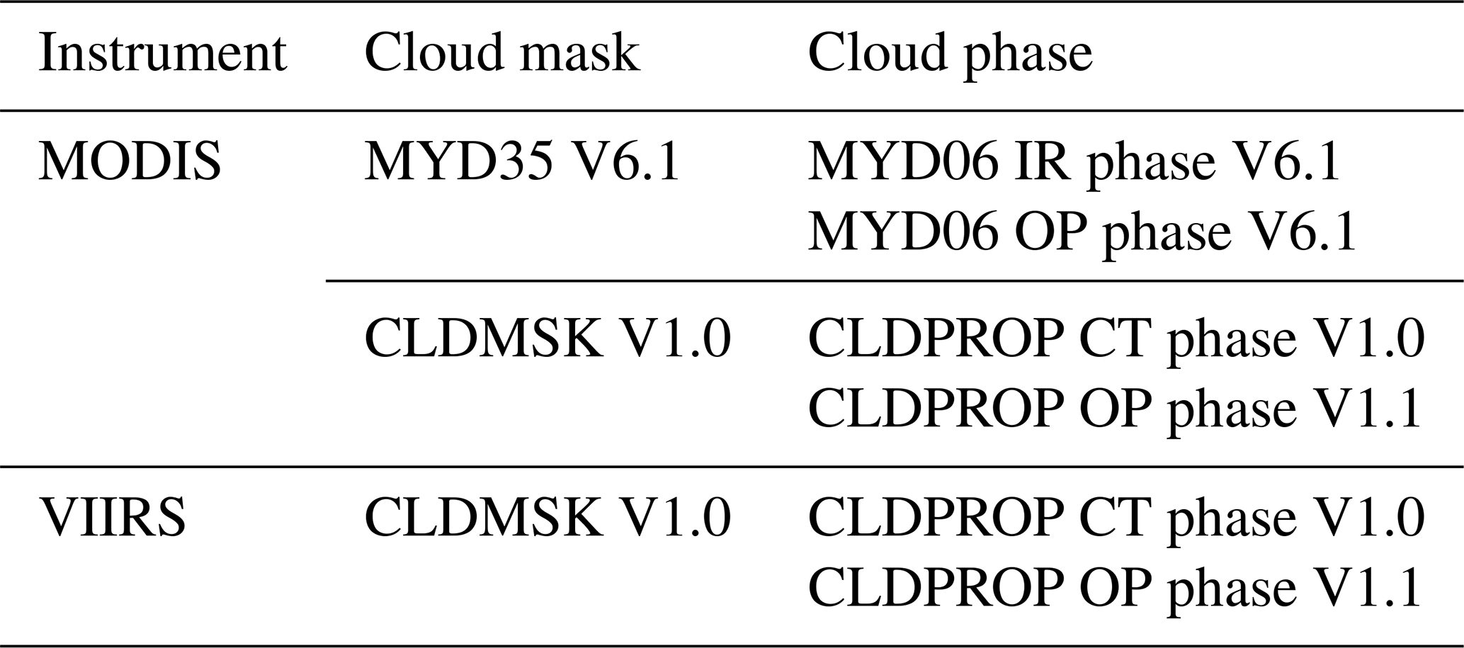
The CLDMSK and MYD35 algorithms use a variety of band combinations and thresholds depending on cloud and surface types (Frey et al., 2008; Ackerman et al., 2008). Meanwhile, the algorithms use different approaches for daytime (i.e., solar zenith angle less than 85∘) and nighttime pixels. In the CLDMSK and MYD35 algorithms, pixels are categorized into four categories, namely confidently clear, probably clear, probably cloudy, and cloudy. The CLDPROP and MYD06 algorithms separate cloudy and probably cloudy pixels into liquid water, ice, and unknown phase categories. Specifically, the MYD06 product includes two cloud-phase algorithms: an IR-phase algorithm (Baum et al., 2012) that uses observations in four MODIS IR bands for daytime and nighttime phase classification (hereafter referred to as the MYD06 IR phase) and a daytime-only algorithm designed for the cloud optical properties retrievals (Marchant et al., 2016; Platnick et al., 2017a) that uses VNIR–SWIR and IR observations (hereafter referred to as the MYD06 OP phase). A notable change for the VIIRS and MODIS CLDPROP algorithm with respect to the standard MODIS MYD06 algorithm is the replacement of the MYD06 IR phase by a NOAA operational algorithm originally developed for Clouds from AVHRR-Extended (CLAVR-x) (Heidinger et al., 2012) and now applied to VIIRS. This algorithm is used to provide cloud top properties, including thermodynamic phase (hereafter CLDPROP CT phase), in the absence of the MODIS CO2 IR gas absorption bands. IR bands are primarily used in the CLDPROP CT-phase algorithm, while complementary SWIR bands are used when available. The MYD06 OP-phase algorithm, applied to daytime pixels only, is included with only minor alteration (related to cloud top properties changes) in the VIIRS and MODIS CLDPROP product (hereafter referred to as the CLDPROP OP phase).
Although the MYD06 and CLDPROP OP-phase products are developed for “cloudy” and “probably cloudy” pixels from the MYD35 and CLDMSK products, a Clear Sky Restoral (CSR) algorithm (Platnick et al., 2017a) is implemented to remove “false cloudy” pixels from the clear-sky conservative MYD35 and CLDMSK products. Specifically, the CSR uses a set of spectral and spatial reflectance variability tests to remove dust, smoke, and strong sunglint pixels that are erroneously identified as cloudy or probably cloudy by the MYD35 and CLDMSK products (Platnick et al., 2017a). One should keep in mind that the CSR algorithm is only applied for the optical property retrievals. Thus, the MYD35 and CLDMSK, and consequently the MYD06 IR phase and CLDPROP CT phase, may have false cloudy pixels in comparison with CALIOP, while the impact on the MYD06 and CLDPROP OP phase is reduced due to the CSR algorithm. The cloud mask and thermodynamic-phase products used in this study are summarized in Table 1.
Table 1Existing VIIRS and MODIS cloud mask and phase products used for comparison. Note that MYD35 and MYD06 are the standard MODIS Aqua products, and CLDMSK and CLDPROP are the MODIS Aqua and VIIRS common algorithm continuity products.
Here we discuss the training of the all-day and daytime RF models for different surface types. Both shortwave (SW) and IR observations will be used in the daytime models while only IR observations will be used in the all-day models. ML model performance is strongly dependent on the quality of training samples. In this study, the two RF models are trained and tested with simple yet highly confident samples (Sect. 4.2). With this training strategy, the RF models are expected to capture the key spectral features from the pure samples efficiently. As discussed in Sect. 4.4, we conducted a model validation that evaluates performance of the two models for simple cases. Furthermore, an analysis of probability distributions from the RF all-day model is conducted to demonstrate that the RF models have the capacity to recognize spectral features from more than one category when atmospheric columns are more complicated.
4.1 Surface types
RF models are trained for different surface types, defined here by the Collection 6 (C6) MODIS annual IGBP surface type product (MCD12C1), to improve model performance over a single general model for all surface types. Although the MCD12C1 product includes up to 18 surface types, for this work we attempt to reduce the total number of surface types by combining surface types with similar spectral white sky albedos and emissivities, as suggested by Thampi et al. (2017). An annual global IGBP surface type map and surface albedo data from the MODIS MCD12C1 (Sulla-Menashe and Friedl, 2018) and a UW-Madison monthly global land surface emissivity database (Seemann et al., 2008) are used to generate the climatology of land surface white-sky albedo and IR emissivity spectra. The UW-Madison database is derived using input from the MODIS operational land surface emissivity product MOD11 (Wan et al., 2004) at six wavelengths located at 3.8, 3.9, 4.0, 8.6, 11, and 12 µm. A baseline fit method is applied to fill the spectral gaps and provides a more comprehensive IR emissivity dataset at 10 wavelengths from 3.6 to 14.3 µm for global land surface with a 0.05∘ spatial resolution (Seemann et al., 2008). The MODIS MCD12C1 product also provides a white-sky albedo dataset at 0.47, 0.56, 0.66, 0.86, 1.24, 1.64, and 2.13 µm with a 0.05∘ spatial resolution (Sulla-Menashe and Friedl, 2018). The means and standard deviations of surface emissivity and white-sky albedo spectra are shown in Figs. 2a and 3a, respectively, for 16 different land surface types generated from the UW-Madison and MCD12C1 data in 2015. Land surface types with similar IR emissivity and SW white-sky albedo spectra are grouped to reduce to the total number of land surface types to six (forest, cropland, grassland, snow and ice, barren desert, and shrubland), as shown in Figs. 2b–f and 3b–f. Figure 4 shows an example map of the reduced global surface type data generated from the MCD12C1 product for 2015.
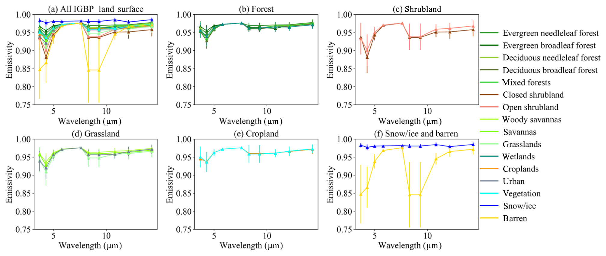
Figure 2Climatology of the spectral surface emissivity data from the UW-Madison baseline fit land surface emissivity database (Seemann et al., 2008) for different IGBP surface types. Error bars indicate the emissivity standard deviations at given wavelengths.
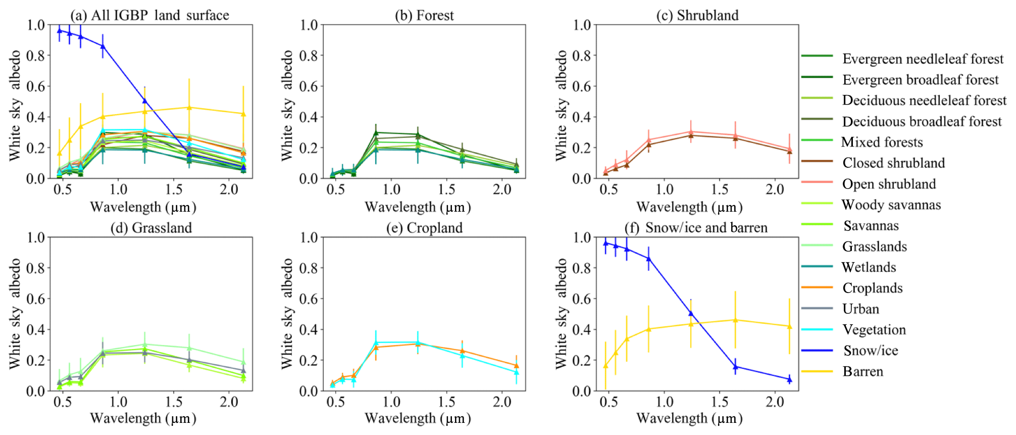
Figure 3Climatology of the spectral surface white sky surface albedo data from MCD12C1 (Sulla-Menashe and Friedl, 2018) for different IGBP surface types. Error bars indicate the albedo standard deviations at given wavelengths.
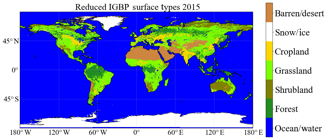
Figure 4A global map of the seven reduced surface types chosen for the RF model training.
4.2 Generating training and validation datasets
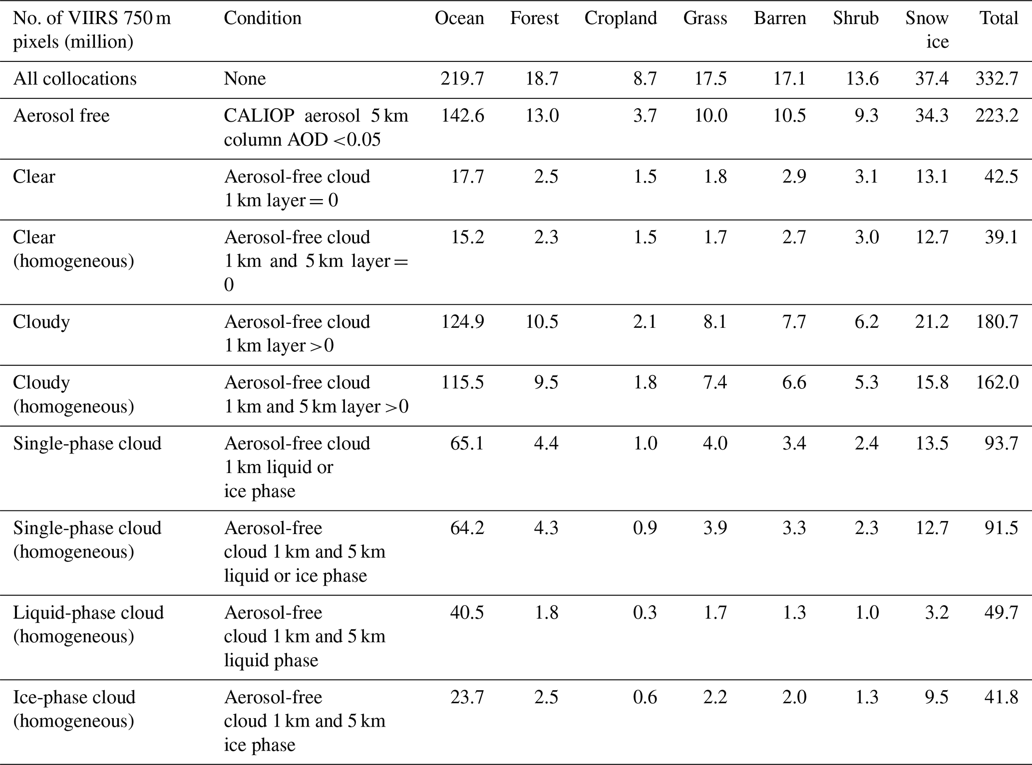
The training and validation data are obtained from a 5-year (2013–2017) SNPP VIIRS and CALIOP collocated dataset. The collected dataset is generated with a collocation algorithm that fully considers the spatial differences between the two instruments and parallax effects, as described in Holz et al. (2008). The SNPP VIIRS data include L1B-calibrated reflectance and brightness temperatures, and the CALIOP data include the 1 km and 5 km cloud and aerosol layer level 2 products. Although more than 332 million VIIRS 750 m pixels are collocated with CALIOP observations, 130.6 million of these pixels (39.3 %) that include only aerosol-free, homogeneous, and clear pixels (39.1 million) or single-phase cloud pixels (49.7 million liquid and 41.8 million ice) are used in our training and validation process. Unless otherwise specified, “aerosol-free” is defined as those pixels having collocated CALIOP 5 km column 532 nm aerosol optical depth less than 0.05, “homogeneous” is defined as those pixels for which the collocated CALIOP 1 km and 5 km products have the same pixel labels, and “single-phase cloud” is defined as those pixels for which the collocated CALIOP 1 km and 5 km products indicate the same thermodynamic phase for all identified cloud layers. More details are given in Table 2.
Table 2Data collection strategies and the number of pixels for all surface types.
A strict three-step quality control process is applied to collect samples for the training and validation process. First, VIIRS 750 m pixels that are potentially contaminated by aerosol are excluded using a threshold of 0.05 column AOD at 532 nm from the level 2 CALIOP 5 km aerosol layer product. Second, each aerosol-free pixel is labeled by one of four categories, namely, “clear sky” and “liquid-water cloud”, “ice cloud”, and “ambiguous” with the L2 CALIOP 1 km and 5 km layer product. The ambiguous pixels, including uncertain and unknown cloud phases from CALIOP and/or overlapping objects belonging to different types (e.g., cirrus over liquid), are discarded. Third, horizontally inhomogeneous pixels, determined when the CALIOP 1 km label changes within five consecutive VIIRS pixels, or pixels with inconsistent CALIOP 1 km and 5 km labels, are discarded. Figure 5 shows the global distributions of the 5-year collocated clear (Fig. 5a–c) and cloudy pixels (Fig. 5d–f) before and after applying the three-step quality control. Globally, 50 % of all clear pixels are excluded due to contamination of broken cloud and/or aerosol. In particular, a large fraction of clear pixels in central Africa, India, and southern China (Fig. 5c) are excluded due to relatively large aerosol optical thicknesses in those regions. About 40 % of global cloudy pixels (Fig. 5f) are excluded due to cloud heterogeneity and aerosol contamination. The minimum selection rate (∼20 %) can be found in some particular regions, such as the Intertropical Convergence Zone (ITCZ), where clouds have complicated horizontal and vertical structures due to strong convections (i.e., clouds are highly heterogeneous in both the horizontal and vertical dimensions). The remaining data are separated into a training and testing population that consists of 32.4, 41.2, and 34.9 million pixels for clear sky, liquid water cloud, and ice cloud from the years 2013–2016, respectively, and a validation dataset that consists of 6.9, 8.5 ,and 7.0 million pixels of clear-sky, liquid water cloud, and ice cloud, respectively, from 2017.
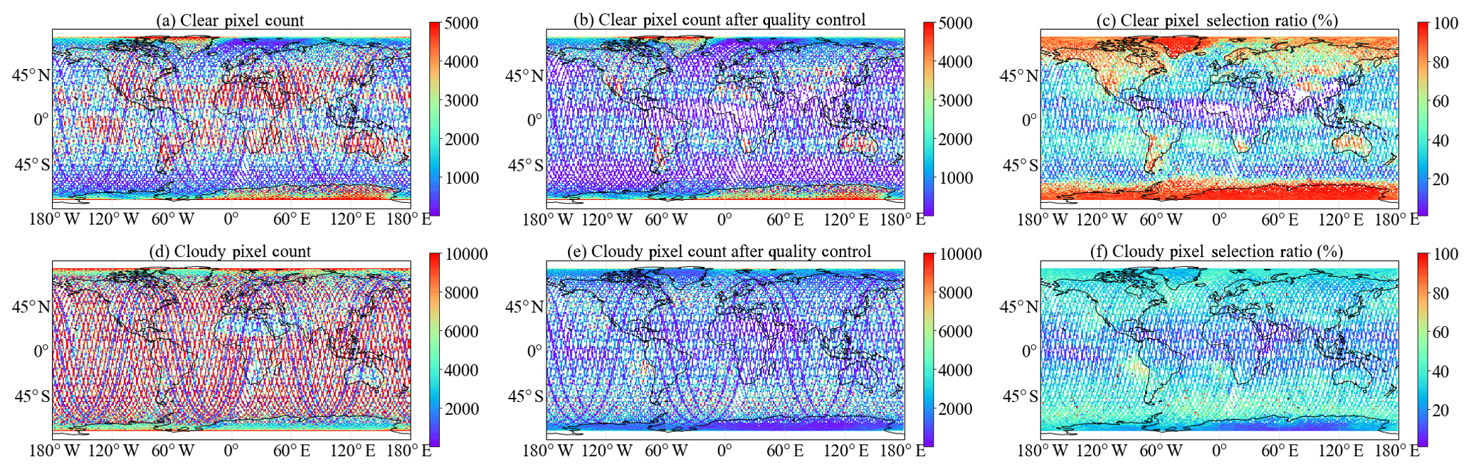
Figure 5Global distributions of the of clear and cloudy pixels from collocated VIIRS and CALIOP data from 2013 to 2017. Panels (a) and (d) show the total clear and cloudy pixel counts, respectively. Panels (b) and (e) show the pixel counts after applying the quality control. The corresponding selection ratios are shown in (c) and (f).
4.3 RF model training and configuration
RF model performance is determined by both its inputs (spectral or other information) and its configuration (NTree and NDepth). Therefore, extensive testing must be conducted to find the optimal inputs and configuration. The 4-year collocated VIIRS-CALIOP dataset from 2013 to 2016 after quality control (see Sect. 4.2) is used for both training (75 %) and testing (25 %) purposes. The testing set, also known as cross-validation set, is used to tune and optimize the RF model parameters. Here we define an accuracy score to evaluate the overall model performance. The accuracy score is the ratio of pixels (samples) where both the CALIOP and RF model have the same categories to total pixels. In this study, we tested six groups of input variables for each RF model. The set of model input variables with a relatively high accuracy score and low memory and computing requirements will be selected.
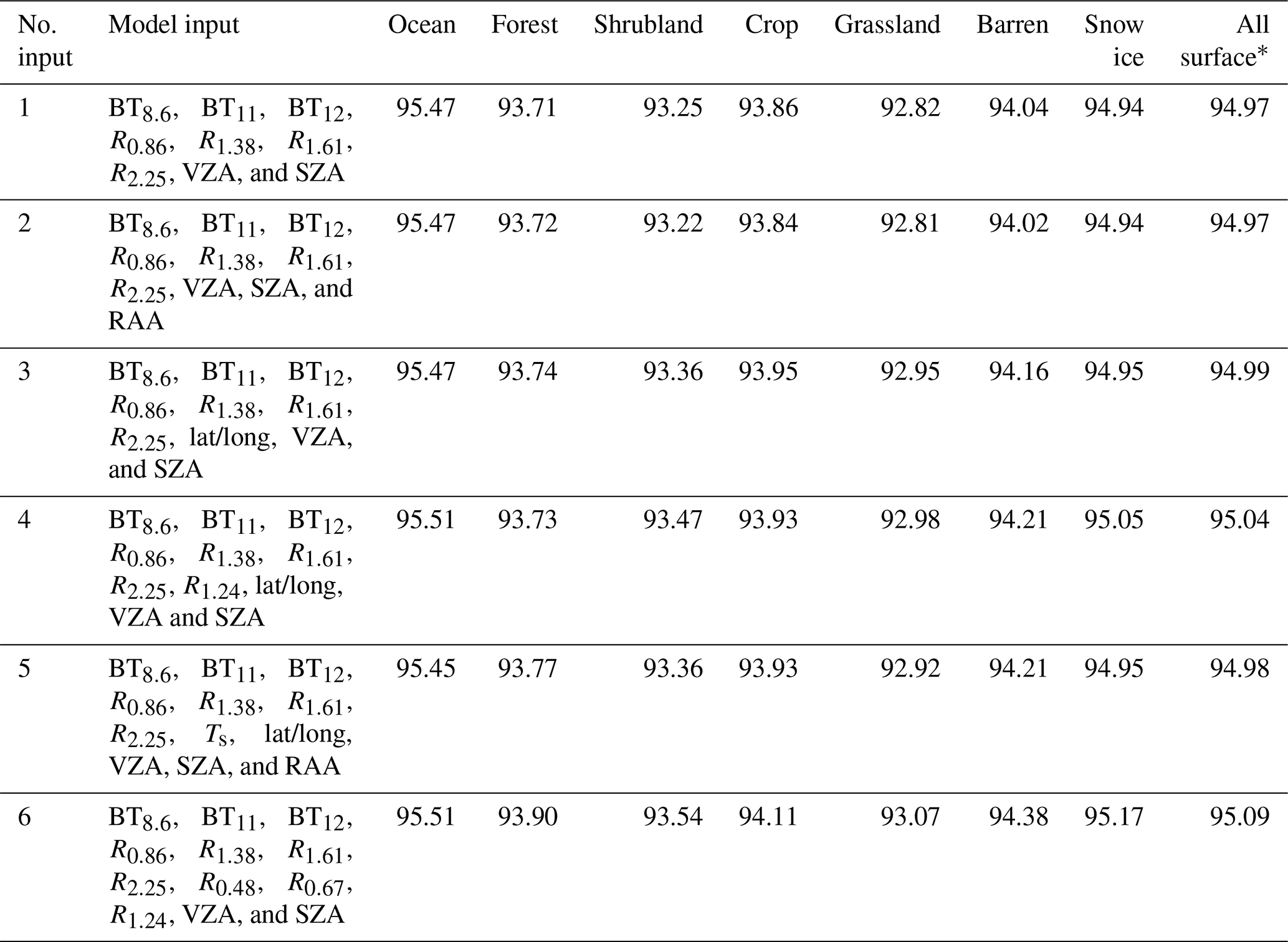
Table 3 provides accuracy scores of the IR-based all-day model trained and tested with different inputs. It shows that with a fixed RF model configuration (NTree=150 and NDepth=15), the RF all-day model with input no. 4 and no. 6 have the best overall accuracy scores for all surface types. Generally, by including surface skin temperature (Ts) and geolocation (i.e., latitude and longitude), the accuracy scores for all surface types increase by 2 %–3 %. The surface emissivity vector εs is less important, likely because this information is highly correlated to surface type and geolocation. In this study, input no. 4 is selected mainly because while it has a similar performance, it requires less memory and computing resources, and it is quite possible that more uncertainty is introduced with the use of a surface emissivity vector εs from another retrieval product.
Table 3Accuracy scores of RF all-day models based on testing pixels with different inputs and a fixed model configuration (NTree =150 and NDepth=15).
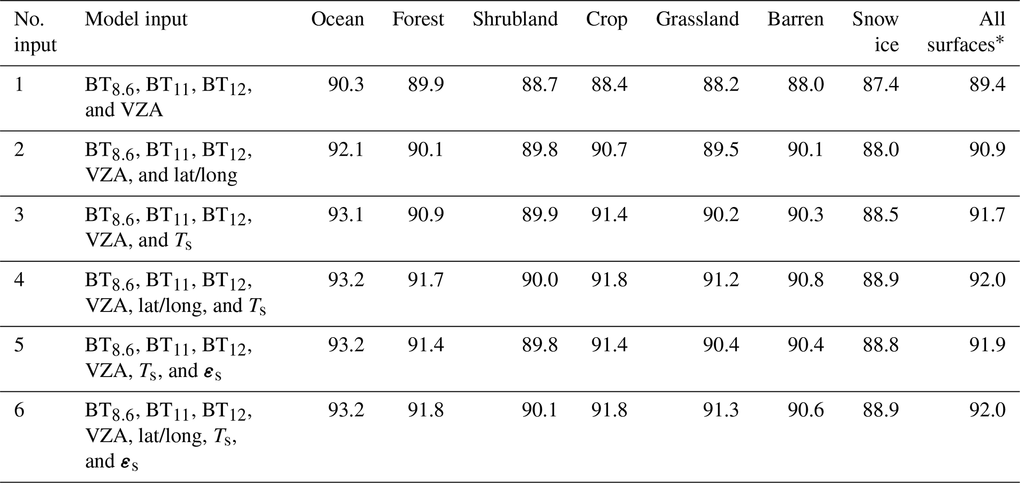
* The all-surface accuracy scores are weighted by pixel numbers of individual surface types.
A set of model configurations (NTree and NDepth) are also tested based on the selected input no. 4. While the number of trees and the maximum depth of individual trees are important determinants for RF model performance, the overall accuracy scores for all surface types are less sensitive to these two model parameters when more than 100 trees and 10 maximum tree depths are used (not shown here). Therefore, we trained the RF all-day models with input no. 4 and the model configuration used in Table 3, i.e., NTree=150 and NDepth=15.
Similar input variable tests for the RF daytime model (IR plus NIR and SWIR observations) showed that the optimal input includes reflectances in the 0.86, 1.24, 1.38, 1.64, and 2.25 µm bands; BTs in the same three IR bands used in the all-day model; geolocation; and solar and satellite-viewing zenith angles (see Table 4). The same model configuration used in the all-day model, e.g., 150 trees with the maximum depth 15, is used in the daytime model. The accuracy scores of the RF daytime model are higher than the RF all-day model by 2 %–3 % over almost all surface types except for high-latitude regions covered by snow and ice, where the daytime model accuracy score is higher by up to 6 % than the all-day model due to the inclusion of the 1.38, 1.64 and 2.25 µm SWIR bands.
Table 4Accuracy scores of RF daytime models based on testing pixels with different inputs and a fixed model configuration (NTree =150 and NDepths=15).
* The all-surface accuracy scores are weighted by pixel numbers of individual surface types.
4.4 Evaluating the RF models
The trained RF all-day and daytime models are validated using collocated CALIOP data in 2017. Existing VIIRS cloud products CLDMSK and CLDPROP (see Table 1) are included for direct comparison with the RF models and CALIOP reference. Several other products, such as the MODIS CLDMSK and CLDPROP and standard MYD35 and MYD06, are also included for comparison, although they could be different from the RF models due to other non-algorithm-based reasons, such as the VZA and pixel size differences mentioned before.
4.4.1 Cloud mask
Cloud mask from the two RF models and VIIRS and MODIS products are first compared with CALIOP lidar observations. For the two models, a cloudy pixel indicates a predicted label “liquid” or “ice”. Here we define cloudy and clear pixels as “positive” and “negative” events, respectively. A true positive rate (TPR) and false positive rate (FPR) can then be used to evaluate model performance. The TPR and FPR are defined as follows:
where TP (true positive) and TN (true negative) are the number of lidar-labeled “cloudy” and “clear” pixels, respectively, that are correctly detected by the models; whereas FN (false negative) and FP (false positive) are the number of lidar-labeled cloudy and clear pixels incorrectly identified by the models. Therefore, TPR, also called model sensitivity, indicates the fraction of all positive events (i.e., lidar cloudy pixels) that are correctly detected by the models. Similarly, FPR, also called false alarm rate, indicates the fraction of all negative events (i.e., lidar clear pixels) that are incorrectly detected as positive (cloudy). TPR and FPR are two critical parameters in model evaluation. A perfect model is associated with a high TPR (close to 1) and a low FPR (close to 0).
Figure 6 shows daytime cloud mask TPR–FPR plots from the two RF models and the other products listed in Table 1. Globally, all products agree well with lidar observations (Fig. 6a). The overall TPRs are higher than 0.94, and FPRs are lower than 0.08. The RF daytime model (red circle), with a TPR of 0.97 and an FPR of 0.05, is slightly better than the RF all-day model (yellow circle) and other products. Figure 6b–h show comparisons over different surface types. It is clear that the RF daytime model has a robust performance for all surface types. The MODIS MYD35 cloud mask algorithm (black circle) performs best over ocean but has a relatively high FPR (0.22) over forest and low TPR over snow and ice and barren (0.85) regions. As mentioned in Sect. 3, the false cloudy pixels from MYD35 and CLDMSK may increase the FPRs correspondingly.

Figure 6False Positive Rate (FPR) versus True Positive Rate (TPR) plots of daytime cloud mask from the two RF models and operational algorithms. Collocated CALIOP level 2 products in 2017 are used as reference. Global comparisons are shown in (a), while panels (b) through (h) show comparisons for difference surface types. The total pixel number is shown in each panel.
The RF all-day model works fairly well and is comparable to other products for all surface types regardless of the fact that it only uses three IR window channels from VIIRS while all other products in the daytime models use VNIR observations. Nighttime (SZA >85∘) cloud mask comparisons are shown in Fig. 7. The overall performances of all operational products decrease in particular for snow and ice regions. For example, the VIIRS and MODIS CLDMSK products over snow and ice surface have large fractions of missing cloudy pixels (e.g., TPRs <0.7) and false alarm rates (FPRs >0.2) over snow and ice surface. The decrease is more likely explained by the lack of SWIR bands and the small cloud–snow (or ice) surface temperature contrast during the nighttime of summer polar regions. However, the RF all-day model has the best performance for nighttime pixels, indicating the strong capability of ML-based algorithm in capturing hidden spectral features and optimizing dynamic thresholds of clear and cloudy pixels.
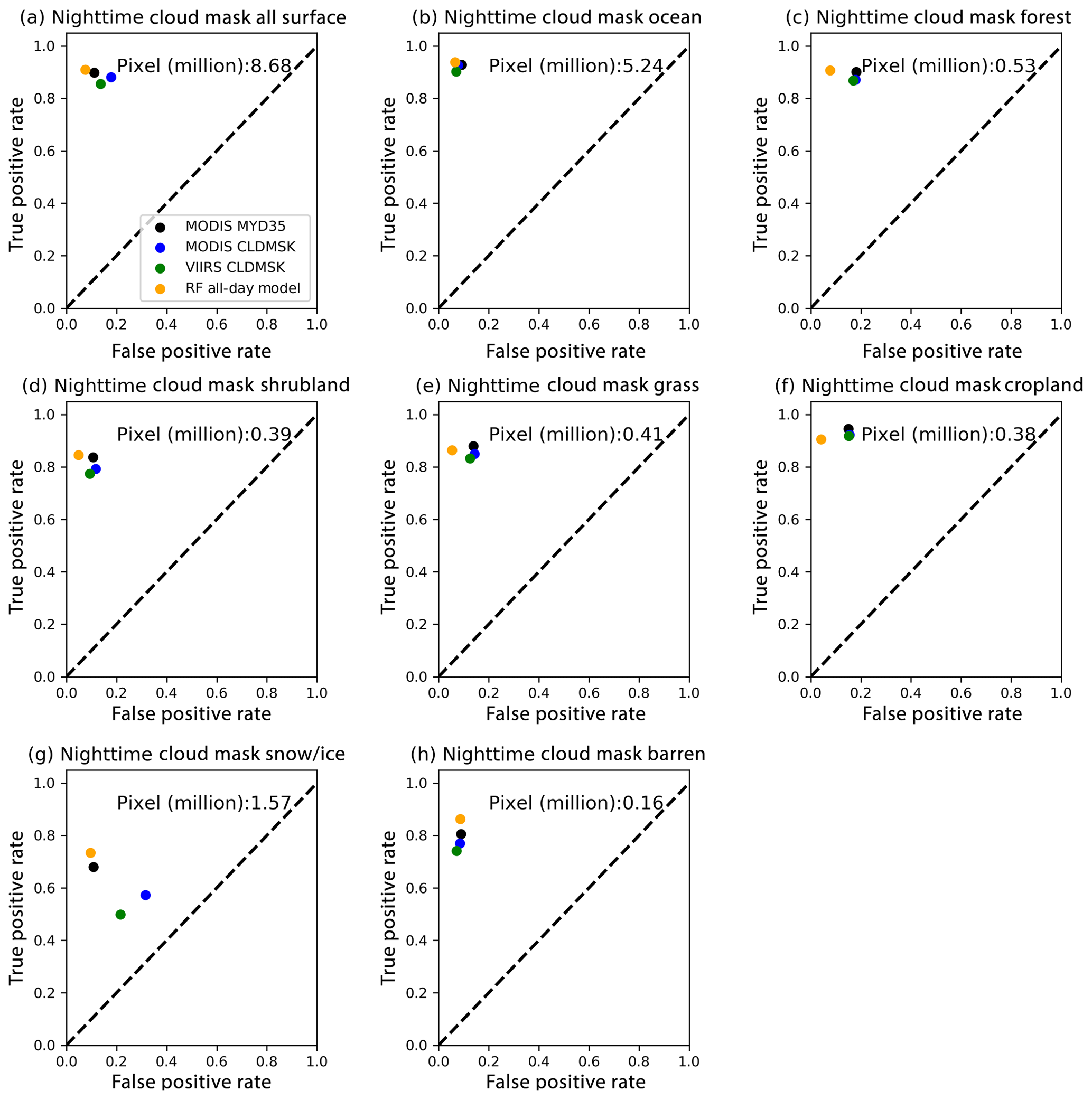
Figure 7Similar to Fig. 6 but for nighttime cloud mask comparisons. The total pixel number is shown in each panel.
4.4.2 Cloud thermodynamic phase
The RF cloud thermodynamic-phase products are also compared with CALIOP lidar and existing VIIRS and MODIS products. For consistent nomenclature, we arbitrarily define ice clouds and liquid water clouds as positive and negative events, respectively. A low TPR indicates an underestimation of ice cloud fraction, while a high FPR indicates that a large fraction of liquid water cloud samples are identified as ice cloud. To focus on cloud thermodynamic-phase classification, pixels detected as clear by either the lidar reference labels or by the RF models and existing products are excluded. The OP phase from both MYD06 and CLDPROP and the IR phase from MYD06 have an “unknown phase” category, which is not included in the TPR–FPR analysis.
Figure 8 shows daytime cloud-phase TPR–FPR plots from the two RF models and the MODIS and VIIRS products. The two RF models and the MODIS MYD06 OP phase are the top three phase algorithms for all surface types. The MODIS MYD06 IR phase, MODIS and VIIRS CLDPROP OP phase, and CT phase have either relatively low TPRs or high FPRs over particular surface types, such as shrubland, snow and ice, and barren regions. Comparisons between nighttime-phase algorithms are shown in Fig. 9. For nighttime clouds, the RF all-day model works better than both CT-phase and IR-phase algorithms for all surface types. Overall, the performance of the hand-tuned algorithms decreases significantly over snow and ice or barren surfaces. For example, the TPR–FPR plot shows that over daytime snow and ice surface (Fig. 8g), the MODIS CLDPROP OP phase and MODIS MYD06 IR phase frequently predict liquid water cloud as ice cloud. Similar to the daytime plot, the MYD06 IR phase also shows a high FPR rate over snow and ice surfaces, indicating an overestimated (underestimated) ice (liquid water) cloud fraction. Possible reasons include strong surface reflection, low surface cloud contrast, relatively few training samples and high solar zenith angles. However, the two RF models work fairly well and show consistent accuracy rates across all surface types.
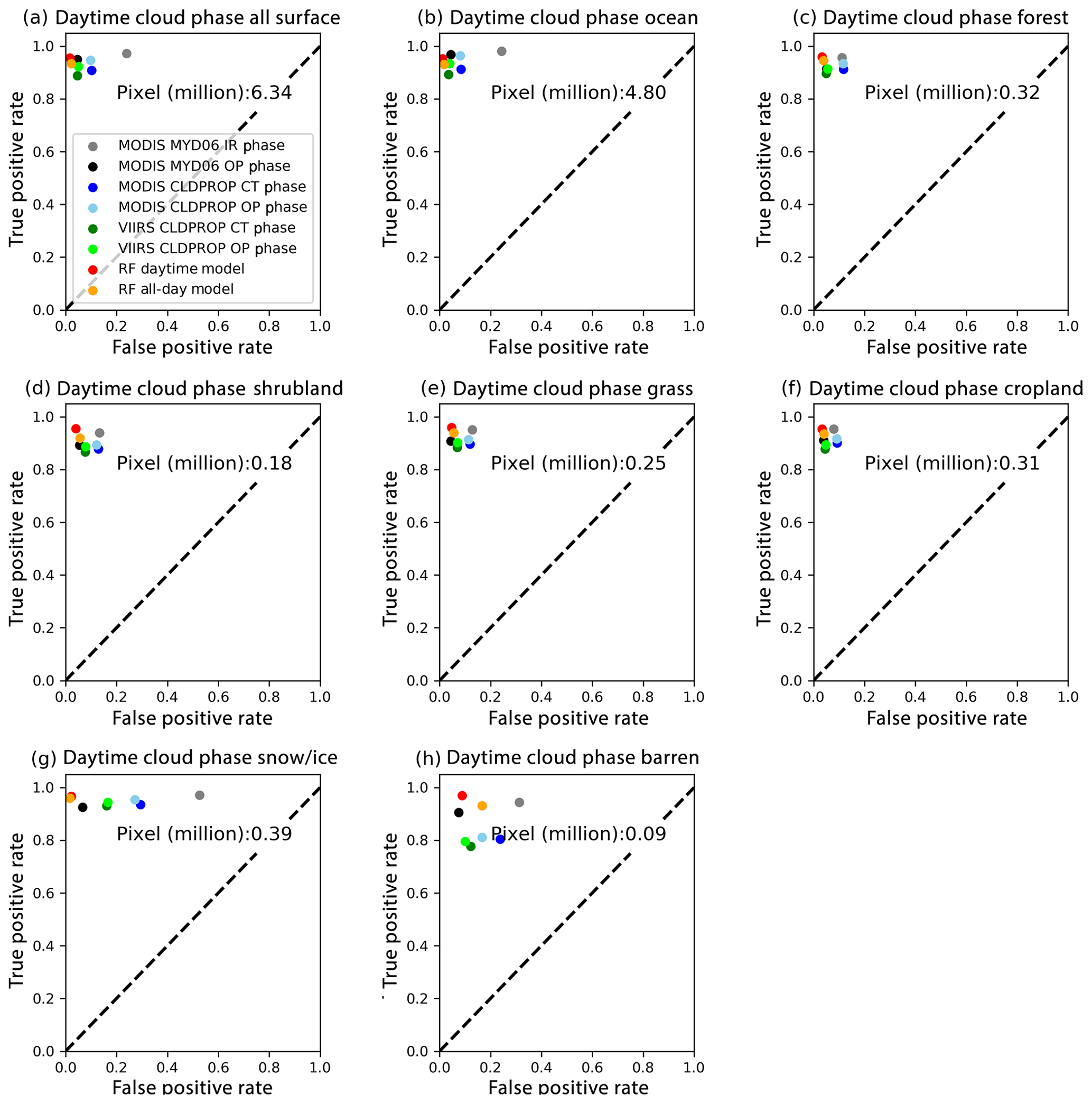
Figure 8Similar to Fig. 6 but for daytime cloud thermodynamic-phase comparisons. The total pixel number is shown in each panel. Note that for specific products, the total pixel numbers are lower because of the exclusion of the unknown phase category (see text for more details).
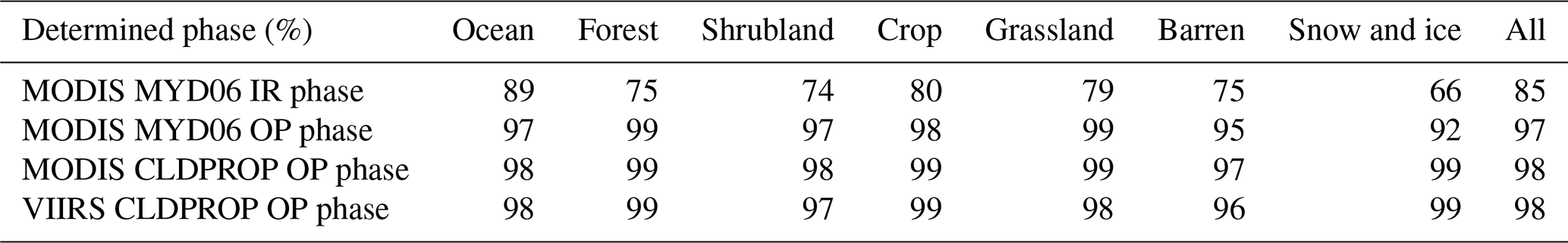
It is also important to note that the number of pixels used for cloud-phase TPR–FPR comparisons in Figs. 8 and 9 are different for products that have unknown phase categories, namely, MYD06 IR phase, MYD06 OP phase, and CLDPROP OP phase. As shown in Table 5, the MYD06 IR phase has a relatively large unknown phase fraction (15 % for all surface types and 34 % for snow and ice) in comparison to the OP-phase products from both MYD06 and CLDPROP, which have approximately 2–3 % unknown phase fraction.
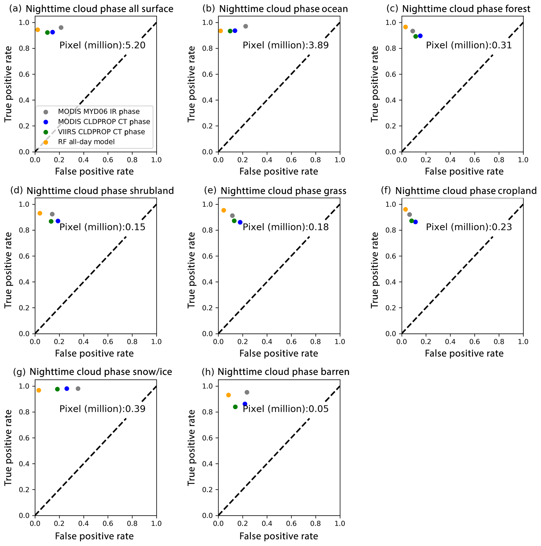
Figure 9Similar to Fig. 6 but for nighttime cloud thermodynamic-phase comparisons. The total pixel number is shown in each panel. Note that for specific products, the total pixel numbers are lower because of the exclusion of the unknown phase category (see text for more details).
Table 5Fractions of the 2017 validation samples that have determined phases (i.e., liquid water or ice) in different surface types.
As discussed in Sect. 2.2, the RF-model-predicted pixel type is derived by setting thresholds on the probabilities for each classification type; e.g., an ice-phase decision is reached if the probability of ice is greater than the probabilities of liquid and clear. Figure 10 shows the probability distribution functions of the RF all-day model for four scene types as determined by collocated CALIOP, namely clear (Fig. 10a), liquid (Fig. 10b), ice (Fig. 10c), and multilayer (Fig. 10d) clouds with different thermodynamic phases (e.g., ice over liquid). As expected, for the first three types, which are included in the training and validation processes, the probability distributions have strong peaks close to either 0 or 1. For the multiple-phase cases (Fig. 10d), the liquid and ice probabilities are more broadly distributed, indicating that the model may recognize signals from both liquid and ice and therefore provide ambiguous phase results. More nuanced thresholds can therefore be applied to the probabilities, for instance to create an unknown phase category following MYD06 and CLDPROP convention (Marchant et al., 2016) that can indicate complicated cloud scenes. Furthermore, the probabilities themselves can provide a useful quality assurance metric for downstream cloud property retrievals that often must make an assumption on cloud phase. Nevertheless, assigning an appropriate phase for downstream imager-based cloud property retrievals is difficult for complex, multilayer cloud scenes, as such an assignment often depends on the optical and microphysical properties and vertical distribution of the cloud layers in the scene (Marchant et al., 2020). Further investigation is necessary to understand how to use the RF-phase probabilities more quantitatively in complicated cases.
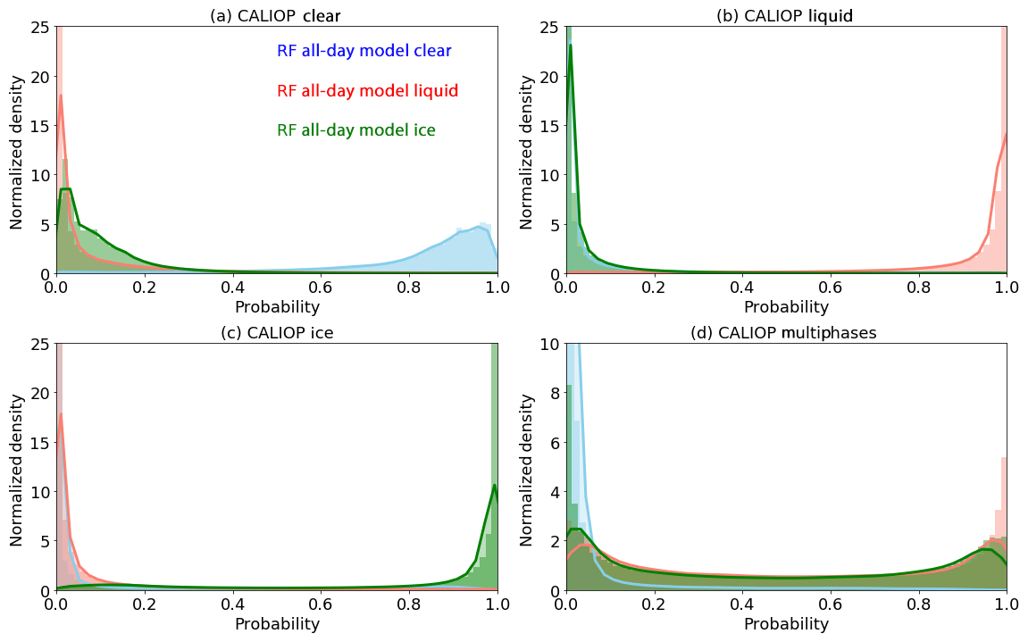
Figure 10Normalized density functions of the clear (blue), liquid water cloud (red), and ice cloud (green) probabilities from the RF all-day model in four CALIOP detected aerosol-free scenes: (a) clear, (b) homogenous liquid, (c) homogenous ice, and (d) multilayer cloud with different thermodynamic phases.
Figure 11 shows monthly mean daytime cloud and phase fractions from the VIIRS CLDMSK and CLDPROP OP-phase products (top row), and those from the RF daytime model (second row), in January 2017. For the cloud mask comparison, cloud fractions (CFs) from the two products have similar spatial patterns, while it is also clear that the VIIRS CLDMSK CFs are higher over tropical oceans by approximately 10 % and lower over land by 5 % (Fig. 11c). This is consistent with the cloud mask TPR–FPR analysis shown in Fig. 6. Over the tropical ocean, the VIIRS CLDMSK is more cloudy, probably due to a fraction of sunglint pixels that are detected as liquid clouds, leading to a large FPR rate. Another reason for the relatively large cloud fraction (or liquid water cloud fraction) difference is that in regions covered by “broken” cumulus clouds and/or clouds with more complicated structures, the inherent viewing geometry differences in the training datasets may adversely affect the performance of the RF models. For example, CALIOP, with a nadir-viewing geometry, may observe clear gaps between two small cloud pieces, while VIIRS, with an oblique viewing angle, detects broken liquid clouds nearby or high clouds along its long line of sight. Comparison between the VIIRS product and the RF daytime model shows more ice clouds from the RF daytime models over land, which is consistent with the cloud-phase TPR–FPR plots as shown in Fig. 8. The RF daytime model may have better performance due to the consideration of surface type. However, it is also important to notice that due to the lack of “aerosol” types in current training, in central Africa, the RF models may misidentify elevated smoke as ice cloudy pixels. For most land surface types, except snow and ice, the CLDPROP OP phase has lower TPR rates than the RF daytime models by 0.1, in comparison with the CALIOP.
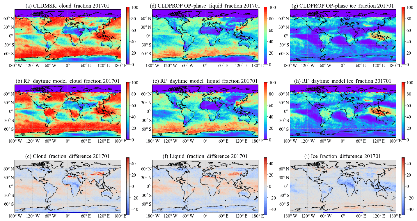
Figure 11Comparisons between 1-month daytime cloud mask and thermodynamic phase products from the VIIRS CLDMSK and CLDPROP OP phase (a, d, g) and the RF daytime model (b, e, h) and their differences (VIIRS–RF daytime, c, f, i) in January 2017.
In addition to the higher CFs over low-latitude ocean from the VIIRS CLDMSK product, more pronounced CF (liquid) differences can be found in northeastern and northwestern China. Cloud differences in the two regions are spatially correlated with locations that have heavy aerosol loadings or snow coverage. For example, heavy aerosol loadings due to pollution in northeastern China, and a wide land snow coverage in northwestern China are frequently observed in the winter. The VIIRS CLDMSK may identify pixels with white surface and heavy aerosol loadings as cloudy. Some of these pixels are expected to be restored to the clear-sky category in the CLDPROP OP-phase product (Fig. 11f and i). As evidence, Fig. 12 shows comparisons between the VIIRS products and the RF daytime model in July 2017. The large cloud (liquid) fraction differences over northern China vanish in the summer. This indicates that the RF models might be able to handle complicated (or unexpected) surface types and strong aerosol events better than the hand-tuned VIIRS algorithm. However, further investigation is required to understand the performances of both the VIIRS products and the RF models.

Figure 12Similar to Fig. 11 but for comparisons in July 2017.
In this section, we will review the strengths and potential limitations and weaknesses of the RF models.
5.1 Advantages
The above results show that, for the screened clear and cloudy samples, the two RF models have better and more consistent performance over different regions and surface types in comparison with the MODIS and VIIRS products, suggesting the potential to improve the overall performance in more global operational applications. In addition to better performance, it is convenient and efficient to apply the present RF models or other similar ML-based models to other instruments similar to VIIRS, such as the geostationary imagers Advanced Himawari Imager (AHI) on Himawari-8/9, the ABI on GOES-16/17, and the Spinning Enhanced Visible and Infrared Imager (SEVIRI) on Meteosat Second Generation, as long as reliable reference pixel labels are available. With hand-tuned methods, adjustment is always required in the case of calibration changes, algorithm porting to another similar instrument, or changes in solar and satellite-viewing geometries and surface conditions. Manual adjustments can be time-consuming (e.g., months or years), whereas the two RF models used in this study were trained and tested for seven surface types and using different input variables for 3 h (on an HPC Platform using 32 Intel Xeon Gold 6126 Processors at 2.60 GHz). More important, manual algorithm adjustment may not provide the best continuity between two instruments. For example, although the MODIS CLDPROP OP phase and VIIRS CLDPROP OP phase are designed for climate record continuity purpose, cloud thermodynamic phases from the two products are different by up to 4 % for all surface pixels and by up to 10 % over surfaces covered by snow and ice (see Fig. 8 light blue and light green dots). Further investigation is necessary to understand if a better climate record continuity can be achieved with a uniform training dataset by using ML approaches. Besides providing a discrete category for each pixel, the RF models provide an ensemble of predictions and probabilities of individual categories, which are useful diagnostic variables in evaluating models in complicated scenarios.
5.2 Limitations and possible caveats
Although the evaluation demonstrates that the current RF models are highly consistent with CALIOP, the models may suffer some artifacts due to the quality of the training data and due to sampling issues.
5.2.1 Quality of the training and validation data
The RF models learn spectral structures of cloudy and clear pixels according to the reference labels. As a consequence, the present model performance relies heavily on the quality of CALIOP level 2 data. It is already known that the lidar signal has limitations in detecting the bottom of an optically thick cloud or lower-level clouds underneath an opaque cloud (Sassen and Cho, 1992). Some complicated multiple-phase scenes may be misidentified as simple single-phase scenes due to the penetration limit of CALIOP (e.g., the uppermost ice cloud optical thickness greater than 3). Using combined CALIOP and CloudSat data as reference in the future could be a better way to improve the training and validation datasets (Marchant et al., 2020). However, as noted in that study, CloudSat observations cannot be used without careful filtering since a multilayer scene that is radiatively indistinct from the upper-level cloud layer is not necessarily consistent with multilayer detection detected from a cloud radar.
Additional uncertainties may come from the inconsistency in view angles between the collocated CALIOP labels and VIIRS spectral observations. For instance, CALIOP always has a quasi-nadir-viewing angle (e.g., 3∘), whereas the collocated VIIRS observations have a wide VZA range (e.g., 0∘ to 50∘). A wide VIIRS VZA range in the training dataset improves model performance, especially for predicting VIIRS pixels with large VZAs. However, the difference between the CALIOP and VIIRS viewing geometry could create undesirable artifacts in the training process. As shown in Fig. 11, in the descending areas of the Hadley cell over low-latitude ocean, where marine boundary layer clouds are dominant, there are relatively large CF differences between the CLDMSK and the RF models. A reason for the large liquid cloud fraction differences is that the quality of training datasets decreases in regions covered by broken cumulus clouds and/or clouds with more complicated structures. Further investigation is required to check if the training dataset collection process introduces sampling bias into the training dataset.
5.2.2 Sampling issue
Uneven sampling may also influence the training of RF models. Figure 13 shows the cloud fraction as a function of viewing geometry. Quasi-constant fractions of both liquid and ice clouds are found for all operational products and the RF models when VZAs are smaller than 45∘, except the MODIS MYD06 IR phase, which has a strong VZA dependency. However, liquid (ice) cloud fractions from the two RF models increase (decrease) rapidly at high VZAs (greater than 50∘), which is likely caused by the sampling issue. A significant fraction of the training data (greater than 98 %) is located in the region with VZA less than 50∘ (see the dashed gray distributions in Fig. 13). It is difficult to mitigate this issue using collocated VIIRS-CALIOP data or observations from other similar instruments in the training process. One possible way is using model-generated synthetic training data and labels with reliable radiative transfer models. Results from the RF daytime model are not shown in Fig. 13 since they are highly consistent with the RF all-day model.
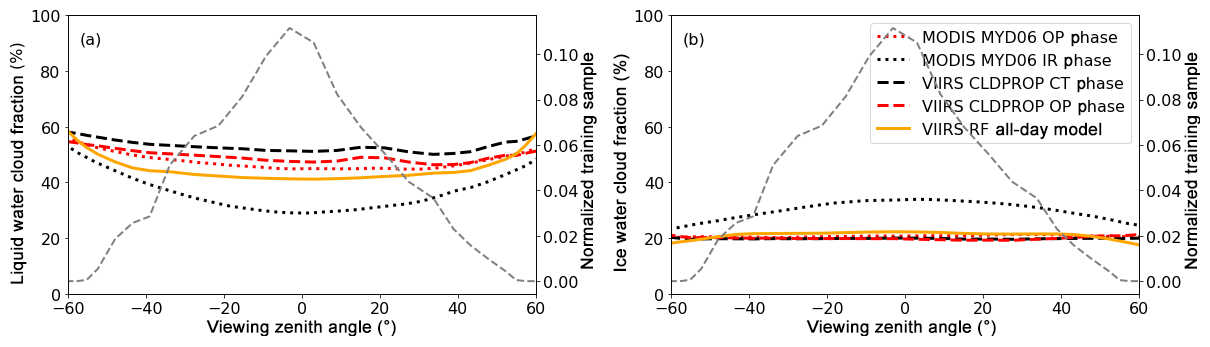
Figure 13Liquid water (a) and ice (b) cloud fractions as a function of viewing zenith angle from the 1-month daytime cloud mask and phase products in January 2017. The dashed gray curve is the probability density function of the 4-year VIIRS and CALIOP training samples (2013–2016).
5.2.3 Labeling strategy
For RF or other ML models, each pixel's classification is determined by prediction probabilities (P) of all potential types. Here we selected a regular strategy that labels a pixel using the class with the highest probability (see Eq. 1). This strategy is logical for problems with two categories (e.g., cloud mask only). For problems including three or more classes, however, the present strategy is not the only way to label pixels. For example, a pixel is labeled as clear if Pclear is larger than both Pliquid and Pice according to the current labeling strategy. It is also possible that, for the same pixel (less than 0.5 % for the two RF models), Pclear is lower than the sum of Pliquid and Pice, making a cloudy label more appropriate. For the cloud mask and phase problem discussed in this paper, in addition to pixel labels, users must be aware of probabilities of the three types. Another possible way to avoid the ambiguous labeling is using two RF models, one for cloud masking and one for phase, such that a clear or cloudy label is given first by the cloud mask model, while a corresponding liquid or ice label is assigned to cloudy pixels in the cloud-phase model. However, two RF models double the training process and require more computing resources in operational applications.
Two machine learning Random Forest (RF) models were trained to provide pixel types (i.e., clear, liquid water cloud, and ice cloud) using VIIRS 750 m spectral observations. A daytime model that uses NIR, SWIR, and IR bands and an all-day model that only uses IR bands were trained separately. In the training processes, reference pixel labels are from collocated CALIOP level 2 1 km cloud layer and 5 km aerosol layer products from 2013 to 2016. Careful tests were conducted to optimize model input and configuration. The two RF models were trained for seven different surface types (i.e., ocean water, forest, cropland, grassland, snow or ice, barren desert, and shrubland) to improve model performance. In addition to geolocation and solar and satellite geometry information, we found that using five NIR and SWIR bands (0.86, 1.24, 1.38, 1.64 and 2.25 µm) and three IR bands (8.6, 11, and 12 µm) in the daytime RF model and using the three IR bands and surface temperatures in the all-day RF model achieved great performances for all surface types.
The cloud mask and thermodynamic-phase classifications from the two RF models were validated using the selected aerosol-free, homogeneous samples in 2017. For daytime cloud mask comparisons over all surface types, the RF daytime model, with a high TPR (0.93 and higher) and low FPR (0.07 and lower), performs best among all models evaluated, including MODIS MYD35 and MODIS and VIIRS CLDMSK products. The RF all-day model works fairly well and is comparable to other products for all surface types, even in daytime when all other products use shortwave observations and it does not. For the nighttime cloud mask, the RF all-day model has the best performance over all products, demonstrating the strong capability of ML-based algorithms for capturing hidden spectral features of clear and cloudy pixels. All nighttime products perform slightly more weakly at snow and ice regions. The decline is likely explained by the lack of SWIR bands and the small thermal contrast between the clouds and the surface during the summer nighttime in polar regions. In this case, the ML-based algorithms are not able to compensate for the missing physical signatures.
For the daytime cloud thermodynamic-phase comparison, we showed that the two RF models are comparable with the MODIS MYD06 OP-phase product and are among the top three phase algorithms for all surface types. The MODIS MYD06 IR phase, VIIRS and MODIS CLDPROP OP phase, and CT phase have either relatively low TPRs or high FPRs over certain surface types, such as shrubland, snow and ice, and barren regions. For nighttime clouds, the RF all-day model works better than both CLDPROP CT phase and MYD06 IR phase for all surface types.
In this study, we have demonstrated the advantages of using ML-based (specifically, RF) models in cloud masking and thermodynamic-phase detection. In contrast with hand-tuned methods, the RF models can be efficiently trained and tested for different surface types and using different input variables. Meanwhile, for aerosol-free, homogeneous samples, the two RF models show better and more consistent performance over different regions and surface types in comparison with existing VIIRS and MODIS datasets. For more complicated scenes, RF probabilities are more informative than binary mask and phase designations. However, further investigation is required to understand how to use probabilities more quantitatively.
In the future, more spectral bands and/or spatial patterns can be used to improve pixel classification skills, such as including more pixel types (e.g., dust and smoke). It is convenient to apply RF models or other similar ML-based models to other instruments similar to VIIRS with the help of active instruments. Most importantly, cloud mask and thermodynamic-phase products from well-trained RF models could be used to train other instruments in the absence of active sensors. For example, the current RF-model-based VIIRS cloud mask and phase data could be used as reference to train ML-based models for other instruments, such as MODIS, ABI, AHI, SEVIRI, and airborne instruments. It remains a goal for future work to determine how such an approach might lead to improved consistency in cloud properties derived from different satellite imagers.
It is also important to emphasize that the model performance is highly reliant on the quality of the training samples and reference labels. For example, in this study, more than 98 % of the training data have a VZA of less than 50∘, leading to more uncertain cloud-phase fractions at large VZAs. Using synthetic training data generated with reliable radiative transfer models could be a possible way to mitigate this artifact.
The Collection 6.1 Aqua/MODIS cloud mask (https://doi.org/10.5067/MODIS/MYD35_L2.061, Ackerman et al., 2017) and cloud thermodynamic phase (https://doi.org/10.5067/MODIS/MYD06_L2.061, Platnick et al., 2015) and the version 1.1 MODIS and VIIRS Continuity cloud mask (https://doi.org/10.5067/MODIS/CLDMSK_L2_MODIS_Aqua.001, Ackerman and Frey, 2019a, and https://doi.org/10.5067/VIIRS/CLDMSK_L2_VIIRS_SNPP.001, Ackerman and Frey, 2019b) and cloud thermodynamic phase (https://doi.org/10.5067/MODIS/CLDPROP_L2_MODIS_Aqua.011, Platnick et al., 2017c and https://doi.org/10.5067/VIIRS/CLDPROP_L2_VIIRS_SNPP.011, Platnick et al., 2017b) are publicly available from NASA and the Atmosphere Archive and Distribution System (LAADS) (https://ladsweb.modaps.eosdis.nasa.gov/search/). The CALIPSO level 2 cloud- and aerosol-layer products (version 4) are publicly available from the Atmospheric Science Data Center (https://opendap.larc.nasa.gov/opendap/CALIPSO/contents.html).
CW developed and tested the RF models. CW created the training and validation datasets with assistance from SP and KM. CW, SP, KM, ZZ, and YZ evaluated the model performance. CW prepared the manuscript with contributions from all co-authors.
The authors declare that they have no conflict of interest.
The authors are grateful for support from the NASA Radiation Sciences Program. Chenxi Wang acknowledges funding support from NASA through the New (Early Career) Investigator Program in Earth Science (grant no.80NSSC18K0749). The computations in this study were performed at the UMBC High Performance Computing Facility (HPCF). The facility is supported by the U.S. National Science Foundation through the MRI program (grant nos. CNS-0821258 and CNS-1228778) and the SCREMS program (grant no. DMS 0821311), with additional substantial support from UMBC.
This research has been supported by the NASA (grant no. 80NSSC18K0749).
This paper was edited by Sebastian Schmidt and reviewed by two anonymous referees.
Ackerman, S. and Frey, R.: Continuity MODIS/Aqua Level-2 (L2) Cloud Mask Product, https://doi.org/10.5067/MODIS/CLDMSK_L2_MODIS_Aqua.001, 2019a.
Ackerman, S. and Frey, R.: Continuity VIIRS/SNPP Level-2 (L2) Cloud Mask Product, https://doi.org/10.5067/VIIRS/CLDMSK_L2_VIIRS_SNPP.001, 2019b.
Ackerman, S. A., Holz, R. E., Frey, R., Eloranta, E. W., Maddux, B. C., and McGill, M.: Cloud detection with MODIS. Part II: Validation, J. Atmos. Ocean. Technol., 25, 1073–1086, https://doi.org/10.1175/2007JTECHA1053.1, 2008.
Ackerman, S., Menzel, P., Frey, R., and Baum, B.: MODIS Atmosphere L2 Cloud Mask Product. NASA MODIS Adaptive Processing System, Goddard Space Flight Center, USA, https://doi.org/10.5067/MODIS/MYD35_L2.061, 2017.
Ackerman, S. A., Frey, R., Heidinger, A., Li, Y., Walther, A., Platnick, S., Meyer, K., Wind, G., Amarasinghe, N., Wang, C., Marchant, B., Holz, R. E., Dutcher, S., and Hubanks, P.: EOS MODIS and SNPP VIIRS Cloud Properties: User guide for climate data record continuity Level-2 cloud top and optical properties product (CLDPROP), version 1, NASA MODIS Adaptive Processing System, Goddard Space Flight Center, USA, 2019.
Baum, B. A., Menzel, W. P., Frey, R. A., Tobin, D. C., Holz, R. E., Ackerman, S. A., Heidinger, A. K., and Yang, P.: MODIS cloud-top property refinements for Collection 6, J. Appl. Meteor. Climatol., 51, 1145–1163, https://doi.org/10.1175/JAMC-D-11-0203.1, 2012.
Breiman, L.: Random forests – random features, Technical report, University of California at Berkeley, Berkeley, California, 1999.
Brodzik, M. J. and Stewart, J. S.: Near-Real-Time SSM/I-SSMIS EASE-Grid Daily Global Ice Concentration and Snow Extent, Version 5, https://doi.org/10.5067/3KB2JPLFPK3R, 2016.
Cao, C., Xiong, J., Blonski, S., Liu, Q., Uprety, S., Shao, X., Bai, Y., and Weng, F.: Suomi NPP VIIRS sensor data record verification, validation, and long-term performance monitoring, J. Geophys. Res.-Atmos., 118, 11664–11678, https://doi.org/10.1002/2013JD020418, 2013.
Cho, H., Nasiri, S. L., and Yang, P.: Application of CALIOP Measurements to the Evaluation of Cloud Phase Derived from MODIS Infrared Channels, J. Appl. Meteor. Climatol., 48, 2169–2180, https://doi.org/10.1175/2009JAMC2238.1, 2009.
Dietterich, T. G.: Ensemble methods in machine learning, International Workshop on Multiple Classifier Systems, MCS 2000, Lecture Notes in Computer Science, vol. 1857, Springer, Berlin, Heidelberg, 2000.
Freund, Y.: An Adaptive Version of the Boost by Majority Algorithm, Machine Learning, 43, 293–318, 2001.
Frey, R. A., Ackerman, S. A., Liu, Y., Strabala, K. I., Zhang, H., Key, J. R., and Wang, X.: Cloud detection with MODIS. Part I: Improvements in the MODIS cloud mask for Collection 5, J. Atmos. Ocean. Technol., 25, 1057–1072, https://doi.org/10.1175/2008JTECHA1052.1, 2008.
Friedman, J. H.: Greedy function approximation: a gradient boosting machine, Ann. Stat., 29, 1189–1232, 2001.
Gelaro, R., McCarty, W., Suárez, M. J., Todling, R., Molod, A., Takacs, L., Randles, C., Darmenov, A., Bosilovich, M. G., Reichle, R., Wargan, K., Coy, L., Cullather, R., Draper, C., Akella, S., Buchard, V., Conaty, A., da Silva, A., Gu, W., Kim, G., Koster, R., Lucchesi, R., Merkova, D., Nielsen, J. E., Partyka, G., Pawson, S., Putman, W., Rienecker, M., Schubert, S. D., Sienkiewicz, M., and Zhao, B.: The Modern-Era Retrospective Analysis for Research and Applications, Version 2 (MERRA-2), J. Climate, 30, 5419–5454, https://doi.org/10.1175/JCLI-D-16-0758.1, 2017.
Hall, D. K. and Riggs, G. A.: MODIS/Aqua Snow Cover Daily L3 Global 500 m SIN Grid, Version 6, NASA National Snow and Ice Data Center Distributed Active Archive Center, Boulder, Colorado USA, https://doi.org/10.5067/MODIS/MYD10A1.006, 2016.
Haynes, J. M., Noh, Y. J., Miller, S. D., Heidinger, A., and Forsythe, J. M.: Cloud geometric thickness and improved cloud boundary detection with GEOS ABI, 15th Annual Symposium on New Generation Operational Environment Satellite Systems, Phoenix, AZ, 6–10 January 2019.
Heidinger, A. K., Evan, A. T., Foster, M. J., and Walther, A.: A naive bayesian cloud-detection scheme derived from CALIPSO and applied within PATMOS-x, J. Appl. Meteor. Climatol., 51, 1129–1144, https://doi.org/10.1175/JAMC-D-11-02.1, 2012.
Ho, T. K: The random subspace method for constructing decision forests, IEEE Trans. Pattern Anal. Mach. Intell, 20, 832–844, 1998.
Holz, R. E., Ackerman, S. A., Nagle, F. W., Frey, R., Dutcher, S., Kuehn, R. E., Vaughan, M. A., and Baum, B.: Global Moderate Resolution Imaging Spectroradiometer (MODIS) cloud detection and height evaluation using CALIOP, J. Geophys. Res., 113, D00A19, https://doi.org/10.1029/2008JD009837, 2008.
Hu, X. F., Belle, J. H., Meng, X., Wildani, A., Waller, L. A., Strickland, M. J., and Liu, Y.: Estimating PM2.5 concentrations in the conterminous United States using the random forest approach, Environ. Sci. Technol., 51, 6936–6944, https://doi.org/10.1021/acs.est.7b01210, 2017.
Ji, C. and Ma, S.: Combinations of weak classifiers, IEEE T. Neural. Networ., 8, 32–42, 1997.
Joachims, T.: Text categorization with support vector machines: Learning with many relevant features, in: Proceedings of the 10th European Conference on Machine Learning, 137–142, Springer-Verlag, Chemnitz, Germany, 1998.
Justice, C. O., Vermote, E., Privette, J., and Sei, A.: The Evolution of U.S. Moderate Resolution Optical Land Remote Sensing from AVHRR to VIIRS. Land Remote Sensing and Global Environmental Change, in: Remote Sensing and Digital Image Processing, edited by: Ramachandran, B., Justice, C., and Abrams, M., 11, Springer, New York, NY, 781–806, 2011.
Kox, S., Bugliaro, L., and Ostler, A.: Retrieval of cirrus cloud optical thickness and top altitude from geostationary remote sensing, Atmos. Meas. Tech., 7, 3233–3246, https://doi.org/10.5194/amt-7-3233-2014, 2014.
Latinne P., Debeir O., and Decaestecker C.: Limiting the number of trees in random forests, in Multiple Classifier Systems, 178–187, Springer-Verlag, Berlin, Germany, 2001.
Lee, T. E., Miller, S. D., Turk, F. J., Schueler, C., Julian, R., Deyo, S., Dills, P., and Wang, S.: The NPOESS VIIRS Day/Night Visible Sensor, B. Am. Meteorol. Soc., 87, 191–200, https://doi.org/10.1175/BAMS-87-2-191, 2006.
Levy, R. C., Mattoo, S., Munchak, L. A., Remer, L. A., Sayer, A. M., Patadia, F., and Hsu, N. C.: The Collection 6 MODIS aerosol products over land and ocean, Atmos. Meas. Tech., 6, 2989–3034, https://doi.org/10.5194/amt-6-2989-2013, 2013.
Liu, Y., Ackerman, S. A., Maddux, B. C., Key, J. R., and Frey, R. A.: Errors in cloud detection over the Arctic using a satellite imager and implications for observing feedback mechanisms, J. Climate, 23, 1894–1907, https://doi.org/10.1175/2009JCLI3386.1, 2010.
Maddux, B. C., Ackerman, S. A., and Platnick, S.: Viewing geometry dependencies in MODIS cloud products, J. Atmos. Ocean. Technol., 27, 1519–1528, https://doi.org/10.1175/2010JTECHA1432.1, 2010.
Martins, J. V., Tanré, D., Remer, L., Kaufman, Y., Mattoo, S., and Levy, R.: MODIS Cloud screening for remote sensing of aerosols over oceans using spatial variability, Geophys. Res. Lett., 29, https://doi.org/10.1029/2001GL013252, 2002.
Marchant, B., Platnick, S., Meyer, K., Arnold, G. T., and Riedi, J.: MODIS Collection 6 shortwave-derived cloud phase classification algorithm and comparisons with CALIOP, Atmos. Meas. Tech., 9, 1587–1599, https://doi.org/10.5194/amt-9-1587-2016, 2016.
Marchant, B., Platnick, S., Meyer, K., and Wind, G.: Evaluation of the Aqua MODIS Collection 6.1 multilayer cloud detection algorithm through comparisons with CloudSat CPR and CALIPSO CALIOP products, Atmos. Meas. Tech. Discuss., https://doi.org/10.5194/amt-2019-448, in review, 2020.
McGill, M. J., Yorks, J. E., Scott, V. S., Kupchock, A. W., and Selmer, P. A.: The Cloud-Aerosol Transport System (CATS): A technology demonstration on the International Space Station, Proc. SPIE, 9612, 96120A, https://doi.org/10.1117/12.2190841, 2015.
Meyer, K., Platnick, S., Arnold, G. T., Holz, R. E., Veglio, P., Yorks, J., and Wang, C.: Cirrus cloud optical and microphysical property retrievals from eMAS during SEAC4RS using bi-spectral reflectance measurements within the 1.88 µm water vapor absorption band, Atmos. Meas. Tech., 9, 1743–1753, https://doi.org/10.5194/amt-9-1743-2016, 2016.
Noel, V., Chepfer, H., Chiriaco, M., and Yorks, J.: The diurnal cycle of cloud profiles over land and ocean between 51∘ S and 51∘ N, seen by the CATS spaceborne lidar from the International Space Station, Atmos. Chem. Phys., 18, 9457–9473, https://doi.org/10.5194/acp-18-9457-2018, 2018.
Oshiro, T. M., Perez, P. S., and Baranauskas, J. A.: How many trees in a random forest, in Machine Learning and Data Mining in Pattern Recognition, MLDM 2012, Lecture Notes in Computer Science, 7376, Springer, Berlin, Heidelberg, 2012.
Pavolonis, M. J., Heidinger, A. K., and Uttal, T.: Daytime global cloud typing from AVHRR and VIIRS: Algorithm description, validation, and comparisons, J. Appl. Meteor. Climatol., 44, 804–826, 2005.
Pedregosa, F., Varoquaux, G., Gramfort, A., Michel, V., Thirion, B., Grisel, O., Blondel, M., Prettenhofer, P., Weiss, R., Dubourg, V., Vanderplas, J., Passos, A., and Cournapeau, D.: Scikit-learn: Machine learning in Python, J. Mach. Learn. Res., 12, 2825–2830, 2011
Platnick, S., King, M., Wind, G., Ackerman, S., Menzel, P., and Frey, R.: MODIS/Aqua Clouds 5-Min L2 Swath 1 km and 5 km, https://doi.org/10.5067/MODIS/MYD06_L2.061, 2015.
Platnick, S., Meyer, K. G., King, M. D., Wind, G., Amarasinghe, N., Marchant, B., Arnold, G. T., Zhang, Z., Hubanks, P. A., Holz, R. E., Yang, P., Ridgway, W. L., and Riedi, J.: The MODIS cloud optical and microphysical products: Collection 6 updates and examples from Terra and Aqua, IEEE T. Geosci. Remote, 55, 502–525, https://doi.org/10.1109/TGRS.2016.2610522, 2017a.
Platnick, S., Meyer, K., Wind, G., Arnold, T., Amrasinghe, N., Marchant, B., Wang, C., Ackerman, S., Heidinger, A., Holtz, B., Li, Y., and Frey, R.: Continuity VIIRS/SNPP Level-2 (L2) Cloud Properties Product, https://doi.org/10.5067/VIIRS/CLDPROP_L2_VIIRS_SNPP.011, 2017b.
Platnick, S., Meyer, K., Wind, G., Arnold, T., Amrasinghe, N., Marchant, B., Wang, C., Ackerman, S., Heidinger, A., Holtz, B., Li, Y., and Frey, R.: Continuity MODIS/Aqua Level-2 (L2) Cloud Properties Product, https://doi.org/10.5067/MODIS/CLDPROP_L2_MODIS_Aqua.011, 2017c.
Remer, L. A., Kaufman, Y. J., Tanré, D., Mattoo, S., Chu, D. A., Martins, J. V., Li, R., Ichoku, C., Levy, R. C., Kleidman, R. G., Eck, T. F., Vermote, E., and Holben, B. N.: The MODIS aerosol algorithm, products, and validation, J. Atmos. Sci., 62, 947–973, https://doi.org/10.1175/JAS3385.1, 2005.
Sassen, K. and Cho, B. S., Subvisual-thin cirrus lidar dataset for satellite verification and climatological research, J. Appl. Meteor., 31, 1275–1285. https://doi.org/10.1175/1520-0450(1992)031<1275:STCLDF>2.0.CO;2, 1992.
Sayer, A. M., Munchak, L. A., Hsu, N. C., Levy, R. C., Bettenhausen, C., and Jeong, M.-J.: MODIS Collection 6 aerosol products: Comparison between Aqua's e-Deep Blue, Dark Target, and “merged” data sets, and usage recommendations, J. Geophys. Res.-Atmos., 119, 13965–13989, https://doi.org/10.1002/2014JD022453, 2014.
Sayer, A. M., Hsu, N. C., Lee, J., Bettenhausen, C., Kim, W. V., and Smirnov, A.: Satellite Ocean Aerosol Retrieval (SOAR) algorithm extension to S-NPP VIIRS as part of the “Deep Blue” aerosol project, J. Geophys. Res.-Atmos., 123, 380–400, https://doi.org/10.1002/2017JD027412, 2017.
Scornet, E.: Tuning parameters in random forests, ESAIM: Procs., 60, 144–162, 2018.
Seemann, S. W., Borbas, E. E., Knuteson, R. O., Stephenson, G. R., and Huang, H.: Development of a global infrared land surface emissivity database for application to clear sky sounding retrievals from multispectral satellite radiance measurements, J. Appl. Meteor. Climatol., 47, 108–123, 2008.
Stephens, G. L., Vane, D. G., Boain, R. J., Mace, G. G., Sassen, K., Wang, Z., Illingworth, A. J., O'connor, E. J., Rossow, W. B., Durden, S. L., Miller, S. D., Austin, R. T., Benedetti, A., Mitrescu, C. M., and the CloudSat team: The CloudSat mission and the A-Train: A new dimension of space-based observations of clouds and precipitation, B. Am. Meteorol. Soc., 83, 1771–1790, 2002.
Strandgren, J., Bugliaro, L., Sehnke, F., and Schröder, L.: Cirrus cloud retrieval with MSG/SEVIRI using artificial neural networks, Atmos. Meas. Tech., 10, 3547–3573, https://doi.org/10.5194/amt-10-3547-2017, 2017.
Stubenrauch, C. J., Rossow, W. B., Kinne, S., Ackerman, S., Cesana, G., Chepfer, H., Di Girolamo, L., Getzewich, B., Guignard, A., Heidinger, A., Maddux, B. C., Menzel, W. P., Minnis, P., Pearl, C., Platnick, S., Poulsen, C., Riedi, J., Sun-Mack, S., Walther, A., Winker, D., Zeng, S., and Zhao, G.: Assessment of Global Cloud Datasets from Satellites: Project and Database Initiated by the GEWEX Radiation Panel, B. Am. Meteorol. Soc., 94, 1031–1049, https://doi.org/10.1175/BAMS-D-12-00117.1, 2013.
Sulla-Menashe, D. and Friedl, M. A.: User Guide to Collection 6 MODIS Land Cover (MCD12Q1 and MCD12C1) Product, USGS, Reston, VA, USA, 2018.
Tanelli, S., Durden, S. L., Im, E., Pak, K., Reinke, D., Partain, P., Haynes, J., and Marchand, R.: CloudSat's cloud profiling radar after two years in orbit: Performance, calibration, and processing, IEEE T. Geosci. Remote, 46, 3560–3573, https://doi.org/10.1109/TGRS.2008.2002030, 2008.
Thampi, B. V., Wong, T., Lukashin, C., and Loeb, N. G.: Determination of CERES TOA fluxes using machine learning algorithms. Part I: Classification and retrieval of CERES cloudy and clear scenes, J. Atmos. Ocean. Technol., 34, 2329–2345, https://doi.org/10.1175/JTECH-D-16-0183.1, 2017.
Tumer, K., and Ghosh, J.: Error correlation and error reduction in ensemble classifiers, Connect. Sci., 8, 385–403, https://doi.org/10.1080/095400996116839, 1996.
Wan, Z., Zhang, Y., Zhang, Q., and Li, Z.-L.: Quality assessment and validation of the MODIS global land surface temperature, Int. J. Remote Sens., 25, 261–274, https://doi.org/10.1080/0143116031000116417, 2004.
Wang, C., Yang, P., Dessler, A., Baum, B. A., and Hu, Y.: Estimation of the cirrus cloud scattering phase function from satellite observations, J. Quant. Spectrosc. Ra., 138, 36–49, https://doi.org/10.1016/j.jqsrt.2014.02.001, 2014.
Wang, C., Platnick, S., Zhang, Z., Meyer, K., and Yang, P.: Retrieval of ice cloud properties using an optimal estimation algorithm and MODIS infrared observations: 1. Forward model, error analysis, and information content, J. Geophys. Res-Atmos., 121, 5809–5826, https://doi.org/10.1002/2015jd024526, 2016a.
Wang, C., Platnick, S., Zhang, Z., Meyer, K., Wind, G., and Yang, P.: Retrieval of ice cloud properties using an optimal estimation algorithm and MODIS infrared observations: 2. Retrieval evaluation, J. Geophys. Res.-Atmos., 121, 5827–5845, https://doi.org/10.1002/2015jd024528, 2016b.
Wang, C., Platnick, S., Fauchez, T., Meyer, K., Zhang, Z., Iwabuchi, H., and Kahn, B. H.: An assessment of the impacts of cloud vertical heterogeneity on global ice cloud data records from passive satellite retrievals, J. Geophys. Res.-Atmos., 124, 1578–1595, https://doi.org/10.1029/2018JD029681, 2019.
Winker, D. M., Tackett, J. L., Getzewich, B. J., Liu, Z., Vaughan, M. A., and Rogers, R. R.: The global 3-D distribution of tropospheric aerosols as characterized by CALIOP, Atmos. Chem. Phys., 13, 3345–3361, https://doi.org/10.5194/acp-13-3345-2013, 2013.
Wolters, E. L., Roebeling, R. A., and Feijt, A. J.: Evaluation of cloud-phase retrieval methods for SEVIRI on Meteosat-8 using ground-based lidar and cloud radar data, J. Appl. Meteor. Climatol., 47, 1723–1738, https://doi.org/10.1175/2007JAMC1591.1, 2008.
Wu, Y., de Graaf, M., and Menenti, M.: Improved MODIS Dark Target aerosol optical depth algorithm over land: angular effect correction, Atmos. Meas. Tech., 9, 5575–5589, https://doi.org/10.5194/amt-9-5575-2016, 2016.
Yuan, T., Wang, C., Song, H., Platnick, S., Meyer, K., and Oreopoulos, L.: Automatically finding ship tracks to enable large-scale analysis of aerosol-cloud interactions, Geophys. Res. Lett., 46, 7726–7733, https://doi.org/10.1029/2019GL083441, 2019.