the Creative Commons Attribution 4.0 License.
the Creative Commons Attribution 4.0 License.
 | 28 May 2020
N2O isotopocule measurements using laser spectroscopy: analyzer characterization and intercomparison
Stephen J. Harris
Jesper Liisberg
Longlong Xia
Kerstin Zeyer
Longfei Yu
Matti Barthel
Benjamin Wolf
Bryce F. J. Kelly
Dioni I. Cendón
Thomas Blunier
Johan Six
For the past two decades, the measurement of nitrous oxide (N2O) isotopocules – isotopically substituted molecules 14N15N16O, 15N14N16O and 14N14N18O of the main isotopic species 14N14N16O – has been a promising technique for understanding N2O production and consumption pathways. The coupling of non-cryogenic and tuneable light sources with different detection schemes, such as direct absorption quantum cascade laser absorption spectroscopy (QCLAS), cavity ring-down spectroscopy (CRDS) and off-axis integrated cavity output spectroscopy (OA-ICOS), has enabled the production of commercially available and field-deployable N2O isotopic analyzers. In contrast to traditional isotope-ratio mass spectrometry (IRMS), these instruments are inherently selective for position-specific 15N substitution and provide real-time data, with minimal or no sample pretreatment, which is highly attractive for process studies.
Here, we compared the performance of N2O isotope laser spectrometers with the three most common detection schemes: OA-ICOS (N2OIA-30e-EP, ABB – Los Gatos Research Inc.), CRDS (G5131-i, Picarro Inc.) and QCLAS (dual QCLAS and preconcentration, trace gas extractor (TREX)-mini QCLAS, Aerodyne Research Inc.). For each instrument, the precision, drift and repeatability of N2O mole fraction [N2O] and isotope data were tested. The analyzers were then characterized for their dependence on [N2O], gas matrix composition (O2, Ar) and spectral interferences caused by H2O, CO2, CH4 and CO to develop analyzer-specific correction functions. Subsequently, a simulated two-end-member mixing experiment was used to compare the accuracy and repeatability of corrected and calibrated isotope measurements that could be acquired using the different laser spectrometers.
Our results show that N2O isotope laser spectrometer performance is governed by an interplay between instrumental precision, drift, matrix effects and spectral interferences. To retrieve compatible and accurate results, it is necessary to include appropriate reference materials following the identical treatment (IT) principle during every measurement. Remaining differences between sample and reference gas compositions have to be corrected by applying analyzer-specific correction algorithms. These matrix and trace gas correction equations vary considerably according to N2O mole fraction, complicating the procedure further. Thus, researchers should strive to minimize differences in composition between sample and reference gases. In closing, we provide a calibration workflow to guide researchers in the operation of N2O isotope laser spectrometers in order to acquire accurate N2O isotope analyses. We anticipate that this workflow will assist in applications where matrix and trace gas compositions vary considerably (e.g., laboratory incubations, N2O liberated from wastewater or groundwater), as well as extend to future analyzer models and instruments focusing on isotopic species of other molecules.
- Article
(5948 KB) - Full-text XML
-
Supplement
(9011 KB) - BibTeX
- EndNote


Nitrous oxide (N2O) is a long-lived greenhouse gas with a 100-year global warming potential nearly 300 times that of carbon dioxide (CO2; Forster et al., 2007) and is the largest emission source of ozone-depleting nitrogen oxides in the stratosphere (Ravishankara et al., 2009). In 2019, the globally averaged [N2O] reached approximately 332 ppb compared to the pre-industrial level of 270 ppb (NOAA/ESRL, 2019). While this increase is known to be linked primarily to increased fertilizer use in agriculture (Bouwman et al., 2002; Mosier et al., 1998; Tian et al., 2015), understanding the underlying microbial processes producing and consuming N2O has proved more challenging, and individual source contributions from sectors such as agricultural soils, wastewater management and biomass burning to global bottom-up estimates of N2O emissions have large uncertainties (Denman et al., 2007). Stable isotopes are an effective tool for distinguishing N2O sources and determining production pathways, which is critical for developing appropriate mitigation strategies (Baggs, 2008; Ostrom and Ostrom, 2011; Toyoda et al., 2017).
The N2O molecule has an asymmetric linear structure (NNO), with the following most abundant isotopocules: 14N15N16O (15Nα−N2O); 15N14N16O (15Nβ−N2O); 14N14N18O (18O−N2O); and 14N14N16O (Yoshida and Toyoda, 2000). The terms 15Nα and 15Nβ refer to the respective central and terminal positions of nitrogen (N) atoms in the NNO molecule (Toyoda and Yoshida, 1999). Isotopic abundances are reported in δ notation, where denotes the relative difference in per mil (‰) of the sample versus atmospheric N2 (AIR-N2). The isotope ratio R(15N∕14N) equals x(15N)∕x(14N), with x being the absolute abundance of 14N and 15N, respectively. Similarly, Vienna Standard Mean Ocean Water (VSMOW) is the international isotope-ratio scale for δ18O. In practice, the isotope δ value is calculated from measurement of isotopocule ratios of sample and reference gases, with the latter being defined on the AIR-N2 and VSMOW scales. By extension, δ15Nα denotes the corresponding relative difference of isotope ratios for 14N15N16O∕14N14N16O, and δ15Nβ for 15N14N16O∕14N14N16O. The site-specific intramolecular distribution of 15N within the N2O molecule is termed 15N-site preference (SP) and is defined as (Yoshida and Toyoda, 2000). The term δ15Nbulk is used to express the average δ15N value and is equivalent to .
Extensive evidence has shown that SP, δ15Nbulk and δ18O can be used to differentiate N2O source processes and biogeochemical cycling (Decock and Six, 2013; Denk et al., 2017; Heil et al., 2014; Lewicka-Szczebak et al., 2014, 2015; Ostrom et al., 2007; Sutka et al., 2003, 2006; Toyoda et al., 2005, 2017; Wei et al., 2017). Isotopocule abundances have been measured in a wide range of environments, including the troposphere (Harris et al., 2014; Röckmann and Levin, 2005; Toyoda et al., 2013), agricultural soils (Buchen et al., 2018; Ibraim et al., 2019; Köster et al., 2011; Mohn et al., 2012; Ostrom et al., 2007; Park et al., 2011; Pérez et al., 2001, 2006; Toyoda et al., 2011; Verhoeven et al., 2018, 2019; Well et al., 2008; Well and Flessa, 2009; Wolf et al., 2015), mixed urban–agricultural environments (Harris et al., 2017), coal and waste combustion (Harris et al., 2015b; Ogawa and Yoshida, 2005), fossil fuel combustion (Toyoda et al., 2008), wastewater treatment (Harris et al., 2015a, b; Wunderlin et al., 2012, 2013), groundwater (Koba et al., 2009; Minamikawa et al., 2011; Nikolenko et al., 2019; Well et al., 2005, 2012), estuaries (Erler et al., 2015), mangrove forests (Murray et al., 2018), stratified water impoundments (Yue et al., 2018), and firn air and ice cores (Bernard et al., 2006; Ishijima et al., 2007; Prokopiou et al., 2017). While some applications like laboratory incubation experiments allow for analysis of the isotopic signature of the pure source, most studies require analysis of the source diluted in ambient air. This specifically applies to terrestrial ecosystem research, since N2O emitted from soils is immediately mixed with background atmospheric N2O. To understand the importance of soil emissions for the global N2O budget, two-end-member mixing models commonly interpreted using Keeling or Miller–Tans plots are frequently used to back-calculate the isotopic composition of N2O emitted from soils (Keeling, 1958; Miller and Tans, 2003).
N2O isotopocules can be analyzed by isotope-ratio mass spectrometry (IRMS) and laser spectroscopic techniques, with currently available commercial spectrometers operating in the mid-infrared (MIR) region to achieve highest sensitivities. IRMS analysis of the N2O intramolecular 15N distribution is based on quantification of the fragmented (NO+, m∕z 30 and 31) and molecular (N2O+, m∕z 44, 45 and 46) ions to calculate isotope ratios for the entire molecule (15N∕14N and 18O∕16O) and the central (Nα) and terminal (Nβ) N atom (Toyoda and Yoshida, 1999). The analysis of N2O SP by IRMS is complicated by the rearrangement of Nα and Nβ in the ion source, while analysis of δ15Nbulk (45∕44) involves correction for NN17O (mass 45). IRMS can achieve repeatability as good as 0.1 ‰ for δ15N, δ18O, δ15Nα and δ15Nβ (Potter et al., 2013; Röckmann and Levin, 2005), but an interlaboratory comparison study showed substantial deviations in measurements of N2O isotopic composition, in particular for SP (up to 10 ‰) (Mohn et al., 2014).
The advancement of mid-infrared laser spectroscopic techniques was enabled by the invention and availability of non-cryogenic light sources which have been coupled with different detection schemes, such as direct absorption quantum cascade laser absorption spectroscopy (QCLAS; Aerodyne Research Inc. (ARI); Wächter et al., 2008), cavity ring-down spectroscopy (CRDS; Picarro Inc.; Berden et al., 2000) and off-axis integrated cavity output spectroscopy (OA-ICOS; ABB – Los Gatos Research Inc.; Baer et al., 2002) to realize compact field-deployable analyzers. In short, the emission wavelength of a laser light source is rapidly and repetitively scanned through a spectral region containing the spectral lines of the target N2O isotopocules. The laser light is coupled into a multi-path cell filled with the sample gas, and the mixing ratios of individual isotopic species are determined from the detected absorption using Beer's law. The wavelengths of spectral lines of N2O isotopocules with distinct 17O, 18O or position-specific 15N substitution are unique due to the existence of characteristic rotational–vibrational spectra (Rothman et al., 2005). Thus, unlike IRMS, laser spectroscopy does not require mass-overlap correction. However, the spectral lines may have varying degrees of overlap with those of other gaseous species, which, if unaccounted for, may produce erroneous apparent absorption intensities. One advantage of laser spectroscopy is that instruments can analyze the N2O isotopic composition in gaseous mixtures (e.g., ambient air) in a flow-through mode, providing real-time data with minimal or no sample pretreatment, which is highly attractive to better resolve the temporal complexity of N2O production and consumption processes (Decock and Six, 2013; Heil et al., 2014; Köster et al., 2013; Winther et al., 2018).
Despite the described inherent benefits of laser spectroscopy for N2O isotope analysis, applications remain challenging and are still scarce for four main reasons:
- 1.
Two pure N2O isotopocule reference materials (USGS51, USGS52) have only recently been made available through the United States Geological Survey (USGS) with provisional values assigned by the Tokyo Institute of Technology (Ostrom et al., 2018). The lack of N2O isotopocule reference materials was identified as a major reason limiting interlaboratory compatibility (Mohn et al., 2014).
- 2.
Laser spectrometers are subject to drift effects (e.g., due to moving interference fringes), particularly under fluctuating laboratory temperatures, which limits their performance (Werle et al., 1993).
- 3.
If apparent δ values retrieved from a spectrometer are calculated from raw uncalibrated isotopocule mole fractions, referred to here as a δ-calibration approach, an inverse concentration dependence may be introduced. This can arise if the analyzer measurements of isotopocule mole fractions are linear, yet the relationship between measured and true mole fractions has a non-zero intercept (e.g., Griffith et al., 2012; Griffith, 2018), such as due to baseline structures (e.g., interfering fringes; Tuzson et al., 2008).
- 4.
Laser spectroscopic results are affected by mole fraction changes of atmospheric background gases (N2, O2 and Ar), herein called gas matrix effects, due to the difference of pressure-broadening coefficients (Nara et al., 2012) and potentially by spectral interferences from other atmospheric constituents (H2O, CO2, CH4, CO, etc.), herein called trace gas effects, depending on the selected wavelength region. The latter is particularly pronounced for N2O due to its low atmospheric abundance in comparison to other trace gases.
Several studies have described some of the above effects for CO2 (Bowling et al., 2003, 2005; Griffis et al., 2004; Griffith et al., 2012; Friedrichs et al., 2010; Malowany et al., 2015; Pataki et al., 2006; Pang et al., 2016; Rella et al., 2013; Vogel et al., 2013; Wen et al., 2013), CH4 (Eyer et al., 2016; Griffith et al., 2012; Rella et al., 2013) and recently N2O isotope laser spectrometers (Erler et al., 2015; Harris et al., 2014; Ibraim et al., 2018; Wächter et al., 2008). However, a comprehensive and comparative characterization of the above effects for commercially available N2O isotope analyzers is lacking.
Here, we present an intercomparison study of commercially available N2O isotope laser spectrometers with the three most common detection schemes: (1) OA-ICOS (N2OIA-30e-EP, ABB – Los Gatos Research Inc.); (2) CRDS (G5131-i, Picarro Inc.); (3) QCLAS (dual QCLAS and trace gas extractor (TREX)-mini QCLAS, ARI). Performance characteristics including precision, repeatability, drift and dependence of isotope measurements on [N2O] were determined. Instruments were tested for gas matrix effects (O2, Ar) and spectral interferences from enhanced trace gas mole fractions (CO2, CH4, CO, H2O) at various [N2O] to develop analyzer-specific correction functions. The accuracy of different spectrometer designs was then assessed during a laboratory-controlled mixing experiment designed to simulate two-end-member mixing, in which results were compared to calculated expected values, as well as to those acquired using IRMS (δ values) and gas chromatography (GC, N2O concentration). In closing, we provide a calibration workflow that will assist researchers in the operation of N2O and other trace gas isotope laser spectrometers in order to acquire accurate isotope analyses.
2.1 Analytical techniques
Operational details of the laser spectrometers tested in this study, including wavenumber regions, line positions and line strengths of N2O, are provided in Table 1. In Fig. 1, selected N2O rotational lines are shown in combination with the absorption lines of the atmospheric most abundant IR-active trace gases (H2O, CO2, CH4, CO and O3) within the different wavenumber regions used by the analyzers. Figure 1 can be used to rationalize possible spectral interferences within different wavenumber regions.
Table 1Overview of the wavelength regions, line positions and line strengths of N2O isotopocules and key operating parameters for each laser spectrometer tested in this study. NTP stands for normal temperature and pressure.
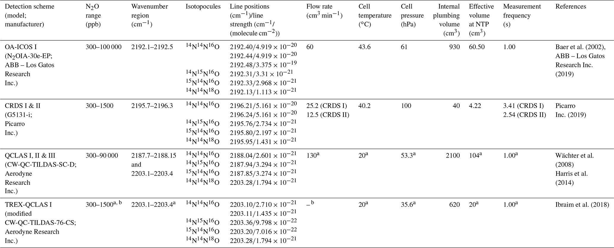
a Dual QC-TILDAS and mini QC-TILDAS are flexible spectrometer platforms, which can be used with different parameter settings. The indicated numbers were chosen for the described experiments. b The mini QC-TILDAS spectrometer is used in combination with a preconcentration device (Ibraim et al., 2018); the indicated N2O concentration range is prior to preconcentration. c The preconcentration – mini QC-TILDAS system is used in a repetitive batch cycle without a continuous sample gas flow (Ibraim et al., 2018, 2019).
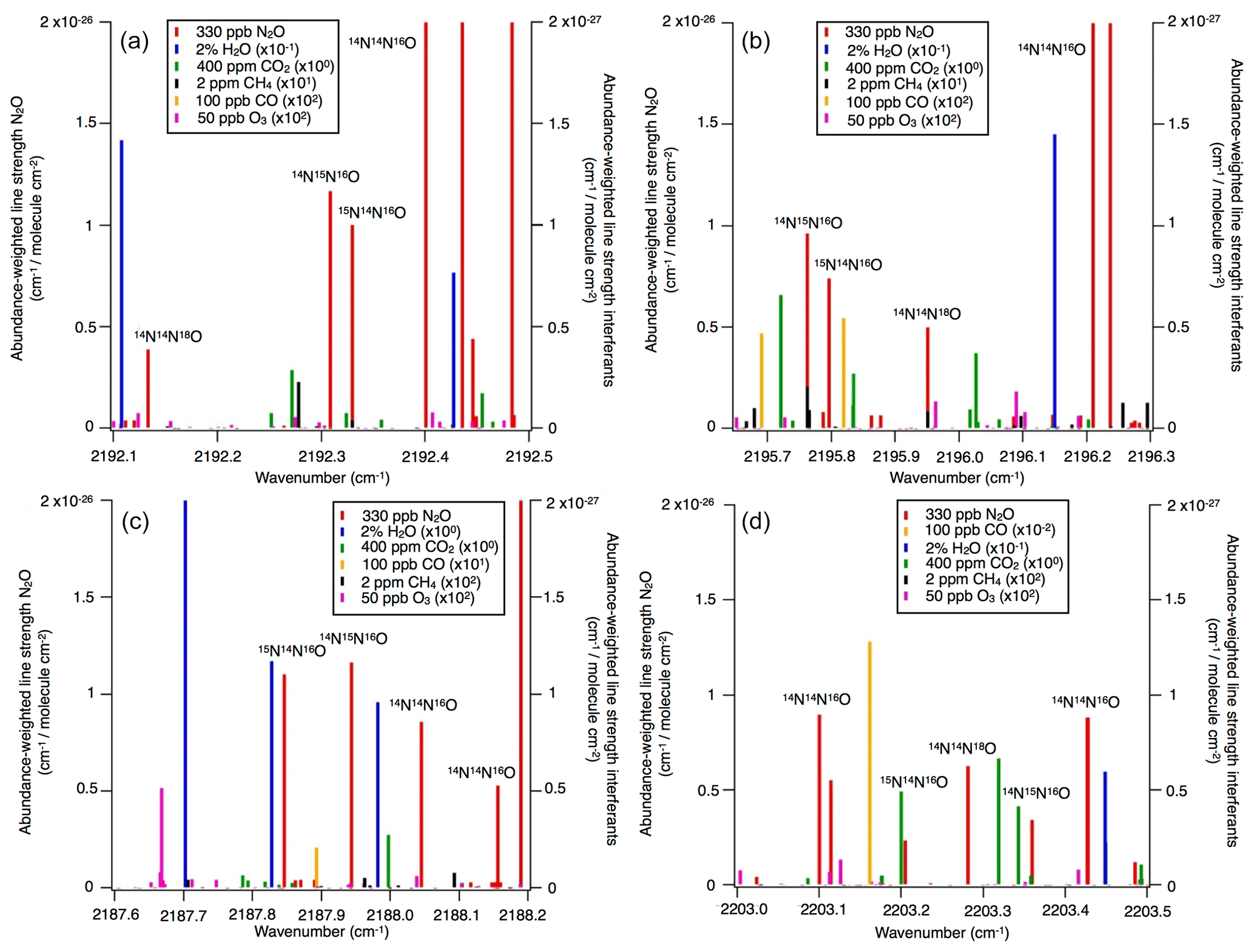
Figure 1N2O isotopocule absorption line positions in the wavenumber regions selected for (a) OA-ICOS, (b) CRDS and (c, d) QCLAS techniques. Regions of possible spectral overlap from interfering trace gases such as H2O, CO2, CH4 and CO are shown. The abundance-scaled line strengths of trace gases have been scaled with 10−1 to 102 (as indicated) because they are mostly weaker than those of the N2O isotopocules.
2.1.1 OA-ICOS (ABB – Los Gatos Research Inc.)
The N2OIA-30e-EP (model 914-0027, serial number 15-830, ABB – Los Gatos Research Inc., USA) tested in this study was provided by the University of New South Wales (UNSW Sydney, Australia) and is herein referred to as OA-ICOS I (Table 1). The instrument employs the OA-ICOS technique integrated with a quantum cascade laser (QCL) (Baer et al., 2002). In short, the QCL beam is directed off axis into the cavity cell with highly reflective mirrors, providing an optical path of several kilometers. For further details on the OA-ICOS technique, the reader is referred to the webpage of ABB – Los Gatos Research Inc. (ABB – Los Gatos Research Inc., 2019) and Baer et al. (2002).
The specific analyzer tested here was manufactured in June 2014 and has had no hardware modifications since then. It is also important to note that a more recent N2OIA-30e-EP model (model 914-0060) is available, that in addition quantifies δ17O. We are unaware of any study measuring N2O isotopocules at natural abundance and ambient mole fractions with the N2OIA-30e-EP. The only studies published so far reporting N2O isotope data apply the N2OIA-30e-EP either at elevated [N2O] in a standardized gas matrix or using 15N labeling, including Soto et al. (2015), Li et al. (2016), Kong et al. (2017), Brase et al. (2017), Wassenaar et al. (2018) and Nikolenko et al. (2019).
2.1.2 CRDS (Picarro Inc.)
Two G5131-i analyzers (Picarro Inc., USA) were used in this study: a 2015 model (referred to as CRDS I, serial number 5001-PVU-JDD-S5001, delivered September 2015) provided by the Niels Bohr Institute, University of Copenhagen, Denmark; and a 2018 model (referred to as CRDS II, serial number 5070-DAS-JDD-S5079, delivered June 2018) provided by Karlsruhe Institute of Technology, Germany (Table 1). In CRDS, the beam of a single-frequency continuous wave (cw) laser diode enters a three-mirror cavity with an effective pathlength of several kilometers to support a continuous traveling light wave. A photodetector measures the decay of light in the cavity after the cw laser diode is shut off to retrieve the mole fraction of N2O isotopocules. For more details, we refer the reader to the webpage of Picarro Inc. (Picarro Inc., 2019) and Berden et al. (2000).
Importantly, the manufacturer-installed flow restrictors were replaced in both analyzer models, as we noted reduced flow rates due to clogging during initial reconnaissance testing. In CRDS I, a capillary (inner diameter, ID: 150 µm, length: 81 mm, flow: 25.2 cm3 min−1) was installed, while CRDS II was equipped with a critical orifice (ID: 75 µm, flow: 12.5 cm3 min−1). Both restrictors were tested and confirmed leakproof. Both analyzers had manufacturer-installed permeation driers located prior to the inlet of the cavity, which were not altered for this study. In December 2017, CRDS I received a software and hardware update as per the manufacturer's recommendations. The CRDS II did not receive any software or hardware upgrades as it was acquired immediately prior to testing.
To the best of our knowledge, the work presented in Lee et al. (2017) and Ji and Grundle (2019) discusses the only published uses of G5131-i models. A prior model (the G5101-i), which employs a different spectral region and does not offer the capability for δ18O, was used by Peng et al. (2014), Erler et al. (2015), Li et al. (2015), Lebegue et al. (2016) and Winther et al. (2018).
2.1.3 QCLAS (Aerodyne Research Inc.)
Three QCLAS instruments (ARI, USA; CW-QC-TILDAS-SC-D) were used in this study. One instrument (QCLAS I, serial number 046), purchased in 2013, was provided by Karlsruhe Institute of Technology, Germany, and two instruments, purchased in 2014 (QCLAS II, serial number 065) and 2016 (QCLAS III, serial number 077), were supplied by ETH Zürich, Switzerland (Table 1). QCLAS I was used in all experiments presented in this study, while QCLAS II and III were only used to assess the reproducibility of drift reported in Sect. 3.1.
All instruments were dual-cw QCL spectrometers, equipped with mirror optics guiding the two laser beams through an optical anchor point to assure precise coincidence of the beams at the detector. On the way to the detector, the laser beams are coupled into an astigmatic multipass cell with a volume of approximately 2100 cm3 in which the beams interact with the sample air. The multiple passes through the absorption cell result in an absorption path length of approximately 204 m. The cell pressure can be selected by the user and was set to 53.3 mbar as a trade-off between line separation and sensitivity. This set point is automatically maintained by the TDL Wintel software (version 1.14.89 ARI, MA, USA), which compensates for variations in vacuum pump speed by closing or opening a throttle valve at the outlet of the absorption cell.
QCLAS instruments offer great liberty to the user as the system can also be operated with different parameter settings, such as the selection of spectral lines for quantification, wavenumber calibration, sample flow rate and pressure. Thereby, different applications can be realized, from high-flow eddy covariance studies or high-mole-fraction process studies to high-precision measurements coupled to a customized inlet system. In addition, spectral interferences and gas matrix effects can be taken into consideration by multi-line analysis, inclusion of the respective spectroscopic parameters in the spectral evaluation or adjustment of the pressure-broadening coefficients. The spectrometers used in this study (QCLAS I–III) were tested under standard settings but were not optimized for the respective experiments. QCLAS I was operated as a single laser instrument using laser 1, to optimize spectral resolution of the frequency sweeps. It is important to note the mixing ratios returned by the instrument are solely based on fundamental spectroscopic constants (Rothman et al., 2005), so that corrections such as the dependence of isotope ratios on [N2O] have to be implemented by the user in the postprocessing.
To our knowledge, QCLAS instruments have so far predominately been used for determination of N2O isotopic composition in combination with preconcentration (see below) or at enhanced mole fractions (Harris et al., 2015a, b; Heil et al., 2014; Köster et al., 2013), except for Yamamoto et al. (2014), who had used a QCLAS (CW-QC-TILDAS-SC-S-N2OISO; ARI, USA) with one laser (2189 cm−1) in combination with a closed chamber system. To achieve the precision and accuracy levels reported in their study, Yamamoto et al. (2014) corrected their measurements for mixing ratio dependence and minimized instrumental drift by measuring N2 gas every 1 h for background correction. These authors also showed that careful temperature control of their instrument in an air-conditioned cabinet was necessary for achieving optimal results.
2.1.4 TREX-QCLAS
A compact mini QCLAS device (CW-QC-TILDAS-76-CS, serial number 074, ARI, USA) coupled with a preconcentration system (TREX) was provided by Empa, Switzerland. The spectrometer comprises a continuous-wave mid-infrared quantum cascade laser source emitting at 2203 cm−1 and an astigmatic multipass absorption cell with a path length of 76 m and a volume of approximately 620 cm3 (Ibraim et al., 2018) (Table 1). The TREX unit was designed and manufactured at Empa and is used to separate the N2O from the sample gas prior to QCLAS analysis. Thereby, the initial [N2O] is increased by a factor of 200–300, other trace gases are removed, and the gas matrix is set to standardized conditions. Before entering the TREX device, CO is oxidized to CO2 using a metal catalyst (Sofnocat 423, Molecular Products Limited, GB). Water and CO2 in sample gases were removed by a permeation dryer (PermaPure Inc., USA) in combination with a sodium hydroxide (NaOH)/magnesium perchlorate (Mg(ClO4)2) trap (Ascarite: 6 g, 10–35 mesh, Sigma Aldrich, Switzerland, bracketed by Mg(ClO4)2, 2×1.5 g, Alfa Aesar, Germany). Thereafter, N2O is adsorbed on a HayeSep D (Sigma Aldrich, Switzerland) filled trap, cooled down to 125.1±0.1 K by attaching it to a copper baseplate mounted on a high-power Stirling cryocooler (CryoTel GT, Sunpower Inc., USA). N2O adsorption requires 5.080±0.011 L of gas to have passed through the adsorption trap. For N2O desorption, the trap is decoupled from the copper baseplate, while slowly heating it to 275 K with a heat foil (diameter 62.2 mm, 100 W, HK5549, Minco Products Inc., USA). Desorbed N2O is purged with 1–5 cm3 min−1 of synthetic air into the QCLAS cell for analysis. By controlling the flow rate and trapping time, the [N2O] in the QCLAS cell can be adjusted to 60–80 ppm at a cell pressure of 35.6±0.04 mbar. A custom-written LabVIEW program (Version 18.0.1, National Instruments Corp., USA) allows remote control and automatic operation of the TREX. So far, the TREX-QCLAS system has been successfully applied to determine N2O emission, as well as N2O isotopic signatures from various ecosystems (e.g., Mohn et al., 2012; Harris et al., 2014; Wolf et al., 2015; Ibraim et al., 2019).
2.1.5 GC-IRMS
IRMS analyses were conducted at ETH Zürich using a gas preparation unit (Trace Gas, Elementar, Manchester, UK) coupled to an IsoPrime100 IRMS (Elementar, Manchester, UK). [N2O] analysis using gas chromatography was also performed at ETH Zürich (456-GC, Scion Instruments, Livingston, UK). GC-IRMS analyses were conducted as part of experiments described further in Sect. 2.4.8. Further analytical details are provided in Sect. S1 in the Supplement.
2.2 Sample and reference gases
2.2.1 Matrix and interference test gases
Table 2 provides O2, Ar and trace gas mole fractions of matrix gases and interference test gases used during testing. The four matrix gases comprised synthetic air (matrix a Messer Schweiz AG, Switzerland); synthetic air with Ar (matrix b, Carbagas AG, Switzerland); synthetic air with Ar, CO2, CH4 and CO at near-ambient mole fractions (matrix c, Carbagas AG, Switzerland); and high-purity nitrogen gas (N2, Messer Schweiz AG, Switzerland). Matrix gases were analyzed in the World Meteorological Organization (WMO) Global Atmosphere Watch (GAW) World Calibration Center at Empa (WCC Empa) for CO2, CH4, H2O (G1301, Picarro Inc., USA), and N2O and CO (CW-QC-TILDAS-76-CS; ARI, USA) against standards of the National Oceanic and Atmospheric Administration/Earth System Research Laboratory/Global Monitoring Division (NOAA/ESRL/GMD). The [N2O] in all matrix gases and N2 were below 0.3 ppb. The three gas mixtures used for testing of spectral interferences contained higher mole fractions of either CO2, CH4 or CO in matrix gas b (Carbagas AG, Switzerland), which prevented spectroscopic analysis of other trace substances.
Table 2O2, Ar content and trace gas concentrations for matrix and interference test gases. Trace gas concentrations of matrix gases were analyzed by WMO GAW WCC Empa against standards of the NOAA/ESRL/GMD. For trace gas concentrations of interference test gases, manufacturer specifications are given. Reported O2 and Ar content is according to manufacturer specifications. The given uncertainty is the uncertainty stated by the manufacturer or the standard deviation for analysis of n cylinders of the same specification.
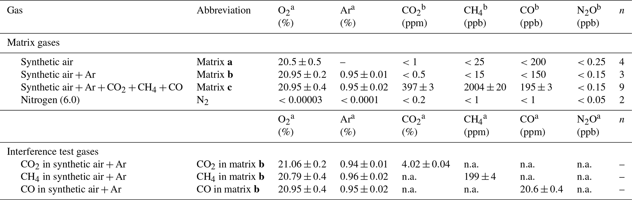
a Manufacturer specifications. b Analyzed at WMO GAW WCC Empa. “n.a.” indicates data not analyzed due to very high concentration of one trace substance, which affects spectroscopic analysis of other species.
2.2.2 Reference gases (S1, S2) and pressurized air (PA1, PA2)
Preparation of pure and diluted reference gases
Two reference gases (S1, S2) with different N2O isotopic composition were used in this study. Pure N2O reference gases were produced from high-purity N2O (Linde, Germany) decanted into evacuated Luxfer aluminum cylinders (S1: P3333N, S2: P3338N) with ROTAREX valves (Matar, Italy) to a final pressure of maximum 45 bar to avoid condensation. Reference gas 1 (S1) was high-purity N2O only. For reference gas 2 (S2), high-purity N2O was supplemented with defined amounts of isotopically pure (>98 %) 14N15NO (NLM-1045-PK), 15N14NO (NLM-1044-PK) (Cambridge Isotope Laboratories, USA) and NN18O using a 10-port two-position valve (EH2C10WEPH with 20 mL sample loop, Valco Instruments Inc., Switzerland). Since NN18O was not commercially available, it was synthesized using the following procedure: (1) 18O exchange of HNO3 (1.8 mL, Sigma Aldrich) with 97 % (5 mL, Medical Isotopes Inc.) under reflux for 24 h; (2) condensation of NH3 and reaction controlled by LN2; and (3) thermal decomposition of NH4NO3 in batches of 1 g in 150 mL glass bulbs with a breakseal (Glasbläserei Möller AG, Switzerland) to produce NN18O. The isotopic enrichment was analyzed after dilution in N2 (99.9999 %, Messer Schweiz AG) with a Vision 1000C quadrupole mass spectrometer (QMS) equipped with a customized ambient pressure inlet (MKS Instruments, UK). Triplicate analysis provided the following composition: 36.25±0.10 % of NN16O and 63.75±0.76 % of NN18O.
High [N2O] reference gases (S1-a90 ppm, S1-b90 ppm, S1-c90 ppm, S2-a90 ppm) with a target mole fraction of 90 ppm were prepared in different matrix gases (a, b, c) using a two-step procedure. First, defined volumes of S1 and S2 were dosed into Luxfer aluminum cylinders (ROTAREX valve, Matar, Italy) filled with matrix gas (a, b and c) to ambient pressure using N2O calibrated mass flow controllers (MFCs) (Vögtlin Instruments GmbH, Switzerland). Second, the N2O was gravimetrically diluted (ICS429, Mettler Toledo GmbH, Switzerland) with matrix gas to the target mole fraction. Ambient [N2O] reference gases (S1-c330 ppb, S2-c330 ppb) with a target mole fraction of 330 ppb were prepared by dosing S1-c90 ppm or S2-c90 ppm into evacuated cylinders with a calibrated MFC, followed by gravimetric dilution with matrix c.
Analysis of reference gases and pressurized air
Table 3 details the trace gas mole fractions and N2O isotopic composition of high and ambient [N2O] reference gases, as well as commercial pressurized air (PA1 and PA2) used during testing. Trace gas mole fractions of high [N2O] reference gases were acquired from the trace gas levels in the respective matrix gases (Table 2), while ambient [N2O] reference gases and target as well as background gases were analyzed by WCC Empa. The isotopic composition of high [N2O] isotope reference gases in synthetic air (S1-a90 ppm, S2-a90 ppm) was analyzed in relation to N2O isotope standards (Cal1–Cal3) in an identical matrix gas (matrix a) using laser spectroscopy (CW-QC-TILDAS-200; ARI, Billerica, USA). The composition of Cal1–Cal3 is outlined in Sect. S2.
Table 3Trace gas concentrations and N2O isotopic composition of high and ambient N2O concentration reference gases, and pressurized air. Trace gas concentrations of high concentration reference gases were retrieved from the composition of matrix gases used for their production (see Table 2); trace gas concentrations in ambient concentration reference gases and pressurized air were analyzed by WMO GAW WCC Empa against standards of the NOAA/ESRL/GMD. The N2O isotopic composition was quantified by laser spectroscopy (QCLAS) and preconcentration – laser spectroscopy (TREX-QCLAS) against reference gases previously analyzed by the Tokyo Institute of Technology.
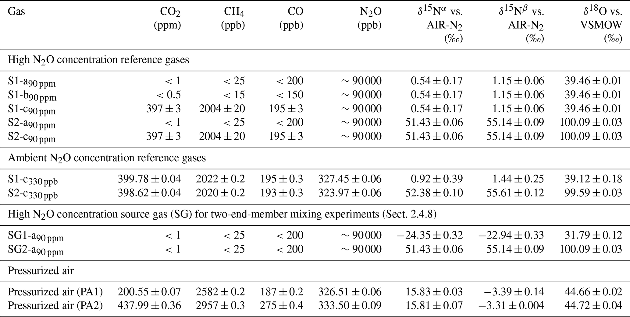
For high-mole-fraction reference gases in matrix b and c (S1-b90 ppm, S1-c90 ppm, S2-c90 ppm), the δ values acquired for S1-a90 ppm and S2-a90 ppm were assigned, since all S1 and S2 reference gases (irrespective of gas matrix) were generated from the same source of pure N2O gas. Direct analysis of S1-b90 ppm, S1-c90 ppm and S2-c90 ppm by QCLAS was not feasible, as no N2O isotope standards in matrix b and c were available. The absence of significant difference (<1 ‰) in N2O isotopic composition between S1-b90 ppm and S1-c90 ppm in relation to S1-a90 ppm (and S2-c90 ppm to S2-a90 ppm) was assured by first statically diluting S1-b90 ppm, S1-c90 ppm and S2-c90 ppm to ambient N2O mole fractions with synthetic air. This was followed by analysis using TREX-QCLAS (as described in Sect. 2.1.4) against the same standards used for S1-a90 ppm, S2-a90 ppm isotope analysis.
Ambient mole fraction N2O isotope reference gases (S1-c330 ppb, S2-c330 ppb) and PA1 and PA2 were analyzed by TREX-QCLAS (Sect. 2.1.4) using N2O isotope standards (Cal1–Cal5) as outlined in Sect. S2.
2.3 Laboratory setup, measurement procedures and data processing
2.3.1 Laboratory setup
All experiments were performed at the Laboratory for Air Pollution/Environmental Technology, Empa, Switzerland, during June 2018 and February 2019. The laboratory was air conditioned to 295 K (±1 K), with ±0.5 K diel variations (Saveris 2, Testo AG, Switzerland), with the exception of a short period (7 to 8 July 2018), where the air conditioning was deactivated to test the temperature dependence of analyzers. Experiments were performed simultaneously for all analyzers, with the exception of the TREX-QCLAS, which requires an extensive measurement protocol and additional time to trap and measure N2O (Ibraim et al., 2018) and thus could not be integrated concurrently with the other analyzers.
Figure 2 shows a generalized experimental setup used for all experiments. Additional information for specific experiments is given in Sect. 2.4, and individual experimental setups are depicted in Sect. S3. Gas flows were controlled using a set of MFCs (model high-performance, Vögtlin Instruments GmbH, Switzerland) integrated into a MFC control unit (Contrec AG, Switzerland). All MFCs were calibrated by the manufacturer for whole air, which according to Vögtlin Instruments is valid for pure N2 and pure O2 as well. Operational ranges of applied MFCs ranged from 0–25 to 0–5000 cm3 min−1 and had reported uncertainties of 0.3 % of their maximum flow and 0.5 % of actual flow. To reduce the uncertainty of the flow regulation, the MFC with the smallest maximum flow range available was selected. The sum of dosed gas flows was always higher than the sum of gas consumption by analyzers, with the overflow exhausted to room air. Gas lines between gas cylinders and MFCs, as well as between MFCs and analyzers, were stainless steel tubing (type 304, Supelco, Sigma Aldrich, Switzerland). Manual two-way (SS-1RS4 or SS-6H-MM, Swagelok, Switzerland) or three-way valves (SS-42GXS6MM, Swagelok, Switzerland) were used to separate or combine gas flows.
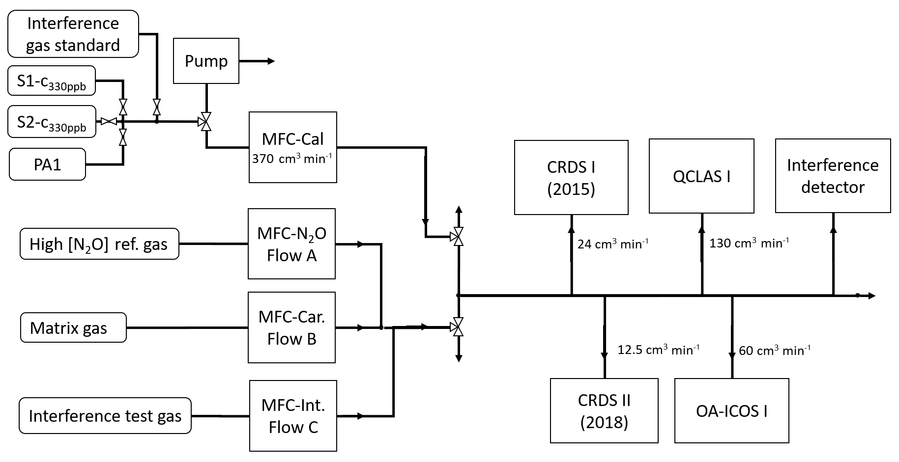
Figure 2The generalized experimental setup used for all experiments conducted in this study. The gases introduced via MFC flows A, B and C were changed according to the experiments outlined in Sect. 2.4. Tables 2 and 3 provide the composition of the matrix gases (MFC B), interference test gases (MFC C) and high [N2O] concentration reference gases (MFC A). Laboratory setups for each individual experiment are provided in Sect. S3.
2.3.2 Measurement procedures, data processing and calibration
With the exception of Allan variance experiments performed in Sect. 2.4.1, all gas mixtures analyzed during this study were measured by the laser spectrometers for a period of 15 min, with the last 5 min used for data processing. Customized R scripts (R Core Team, 2017) were used to extract the 5 min averaged data for each analyzer. Whilst the OA-ICOS and QCLAS instruments provide individual 14N14N16O, 14N15N16O, 15N14N16O and 14N14N18O mole fractions, the default data output generated by the CRDS analyzers are δ values, with underlying calculation schemes inaccessible to the user. Therefore, to remain consistent across analyzers, uncalibrated δ values were calculated for OA-ICOS and QCLAS instruments first, using literature values for the 15N∕14N (0.0036782) and 18O∕16O (0.0020052) isotope ratios of AIR-N2 and VSMOW (Werner and Brand, 2001).
Each experiment was performed over the course of 1 d and consisted of three phases: (1) an initial calibration phase; (2) an experimental phase; and (3) a final calibration phase. During phases (1) and (3), reference gases S1-c330 ppb and S2-c330 ppb were analyzed. On each occasion (i.e., twice a day), this was followed by the analysis of PA1, which was used to determine the long-term (day-to-day) repeatability of the analyzers. Phase (2) experiments are outlined in Sect. 2.4. Throughout all three phases, all measurements were systematically alternated with an Anchor gas measurement, the purpose of which was two-fold: (1) to enable drift correction and (2) as a means of quantifying deviations of the measured [N2O] and δ values caused by increasing [N2O] (Sect. 2.4.4), the removal of matrix gases (O2 and Ar in Sect. 2.4.5) or addition of trace gases (CO2, CH4 and CO in Sect. 2.4.6). Accordingly, the composition of the Anchor gas varied across experiments (see Sect. 2.4) but remained consistent throughout each experiment. A drift correction was applied to the data if a linear or non-linear model fitted to the Anchor gas measurement over the course of an experiment was statistically significant at p<0.05. Otherwise, no drift correction was applied.
In Sect. 2.4.3 (repeatability experiments) and 2.4.8 (two-end-member mixing experiments), trace gas effects were corrected according to Eqs. (1), (2) and (3) using derived analyzer-specific correction functions because the CO2, CH4 and CO composition of PA1 in Sect. 2.4.3 and the gas mixtures in Sect. 2.4.8 varied from those of the calibration gases S1-c330 ppb (S1) and S2-c330 ppb (S2):
and
where [N2O]tc, G and δtc, G refer to the trace-gas-corrected [N2O] and δ values (δ15Nα, δ15Nβ or δ18O) of sample gas G, respectively; [N2O]meas, G and δmeas, G are the raw uncorrected [N2O] and δ values measured by the analyzer for sample gas G, respectively; Δ[N2O] and Δδ refer to the offset on the [N2O] or δ values, respectively, resulting from the difference in trace gas mole fraction between sample gas G and reference gases, denoted Δ[x]G; [x]G is the mole fraction of trace gas x (CO2, CH4 or CO) in sample gas G; and [x]S1 and [x]S2 are the mole fractions of trace gas x in reference gases S1-c330 ppb and S2-c330 ppb. It is important to note that the differences in CO2 and CH4 mole fractions in S1-c330 ppb and S2-c330 ppb are 2 orders of magnitude smaller than the differences with PA1.
Thereafter, δ values of trace-gas-corrected, mole-fraction-corrected (Sect. 2.4.8 only) and drift-corrected measurements from the analyzers were normalized to δ values on the international isotope-ratio scales using a two-point linear calibration procedure derived from values of S1-c330 ppb (S1) and S2-c330 ppb (S2) calculated using Eq. (4) (Gröning, 2018):
where δCal, G is the calibrated δ value for sample gas G normalized to international isotope-ratio scales; δref, S1 and δref, S2 are the respective δ values assigned to reference gases S1-c330 ppb and S2-c330 ppb; δcorr, S1 and δcorr, S2 are the respective δ values measured for the reference gases S1-c330 ppb and S2-c330 ppb which, if required, were drift corrected; and δcorr, G is the trace-gas-corrected, mole-fraction-corrected (Sect. 2.4.8 only) and drift-corrected (if required) δ value measured for the sample gas G.
2.4 Testing of instruments
An overview of all experiments performed in this study, including applied corrections and instruments tested, is provided in Table 4.
Table 4Overview of the experiments performed in this study.
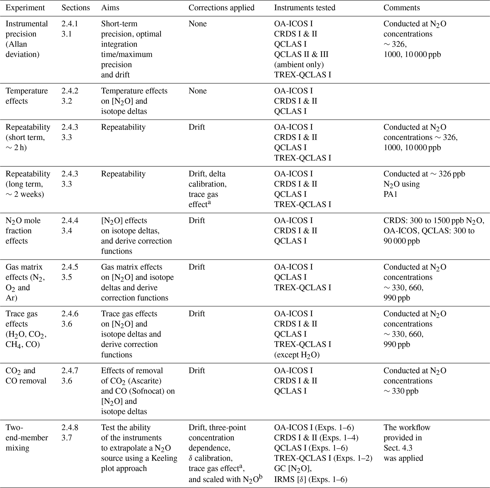
a Derived from trace gas effect determined in Sect. 3.6. b Derived from scaling effects described in Sect. 3.6.2.
2.4.1 Allan precision
The precision of the laser spectrometers was determined using the Allan variance technique (Allan, 1966; Werle et al., 1993). Experiments were conducted at different [N2O]: ambient, 1000 and 10 000 ppb. For the Allan variance testing conducted at ambient [N2O], a continuous flow of PA1 was measured continuously for 30 h. For testing conducted at 1000 and 10 000 ppb [N2O], S1-c90 ppm was dynamically diluted to 1000 or 10 000 ppb [N2O] with matrix gas c for 10 h. CRDS I and II were disconnected for the 10 000 ppb measurement because [N2O] exceeded the specified measurement range. Daily drifts were estimated using the slope of the linear regression over the measurement period normalized to 24 h (i.e., ppb d−1 and ‰ d−1).
2.4.2 Temperature effects
To investigate instrumental sensitivities to variations in ambient temperature, PA1 was simultaneously and continuously measured by all analyzers in flow-through mode for a period of 24 h, while the air conditioning of the laboratory was turned off for over 10 h. This led to a rise in temperature from 21 to 30 ∘C, equating to an increase in temperature of approximately 0.9 ∘C h−1. The increase in laboratory room temperature was detectable shortly after the air conditioning was turned off due to considerable heat being released from several other instruments located in the laboratory. Thereafter, the air conditioning was restarted and the laboratory temperature returned to 21 ∘C over the course of 16 h, equating to a decrease of roughly 0.6 ∘C h−1, with most pronounced effects observable shortly after restart of air conditioning when temperature changes were highest.
2.4.3 Repeatability
Measurements of PA1 were taken twice daily over ∼2 weeks prior to and following the experimental measurement period to test the long-term repeatability of the analyzers. Measurements were sequentially corrected for differences in trace gas concentrations (Eqs. 1–3), drift (if required) and then δ calibrated (Eq. 4). No matrix gas corrections were applied because the N2, O2 and Ar composition of PA1 was identical to that of S1-c330 ppb and S2-c330 ppb. TREX-QCLAS I measurements for long-term repeatability were collected separately from other instruments over a period of 6 months. Repeatability over shorter time periods (2.5 h) was also tested for each analyzer by acquiring 10 repeated 15 min measurements at different N2O mole fractions: ambient (PA1), 1000 and 10 000 ppb N2O.
2.4.4 N2O mole fraction dependence
To determine the effect of changing [N2O] on the measured δ values, S1-c90 ppm was dynamically diluted with matrix c to various [N2O] spanning the operational ranges of the instruments. For both CRDS analyzers mole fractions between 300 to 1500 ppb were tested, while for the OA-ICOS I and QCLAS I mixing ratios ranged from 300 to 90 000 ppb. Between each [N2O] step change, the dilution ratio was systematically set to 330 ppb N2O to perform an Anchor gas measurement. For each instrument, the effect of increasing [N2O] on δ values was quantified by comparing the measured δ values at each step change to the mean measured δ values of the Anchor gas and was denoted Δδ such that and ΔδAnchor=0. The experiment was repeated on three consecutive days to test day-to-day variability.
2.4.5 Gas matrix effects (O2 and Ar)
Gas matrix effects were investigated by determining the dependence of [N2O] and isotope δ values on the O2 or Ar mixing ratio of a gas mixture. For O2 testing, Gases 1, 2 and 3 (N2) were mixed to incrementally change mixing ratios of O2 (0 %–20.5 % O2) while maintaining a consistent [N2O] of 330 ppb (Table 5). As an Anchor gas, Gas 1 (S1-a90 ppm) was dynamically diluted with Gas 2 (matrix a) to produce 330 ppb N2O in matrix a. O2 mole fractions in the various gas mixtures were analyzed with a paramagnetic O2 analyzer (Servomex, UK) and agreed with expected values to within 0.3 % (relative). For Ar testing, Gas 1 (S1-b90 ppm) was dynamically diluted with Gas 2 (matrix b) to produce an Anchor gas with ∼330 ppb N2O in matrix b. Gases 1, 2 and 3 (N2+O2) were then mixed to incrementally change mixing ratios of Ar (0.003 %–0.95 % Ar), while a consistent [N2O] of 330 ppb was maintained. Ar compositional differences were estimated based on gas cylinder manufacturer specifications and selected gas flows. The effects of decreasing O2 and Ar on [N2O] and δ values were quantified by comparing the measured [N2O] and δ values at each step change to the mean measured [N2O] and δ values of the Anchor gas and were denoted Δ[N2O] and Δδ, similar to Sect. 2.4.4. Deviations in O2 and Ar mixing ratios were quantified by comparing the [O2] and [Ar] at each step change to the mean [O2] and [Ar] of the Anchor gas and were denoted ΔO2 and ΔAr such that, for example, and ΔO2 Anchor=0. Both O2 and Ar experiments were triplicated.
In addition, O2 and Ar effects were derived for N2O mole fractions of ∼660 and ∼990 ppb. These experiments were undertaken in a way similar to those described above, except Anchor gas measurements were conducted once (not triplicated).
Table 5Gas mixtures used to test effects of gas matrix (O2, Ar) or trace gases (CO2, CH4 and CO) on [N2O] and isotope deltas. Gas 1 was dynamically diluted with Gas 2 to make up an Anchor gas with [N2O] of ∼330 ppb which was systematically measured throughout the experiments to (1) enable drift correction and (2) quantify deviations of the measured [N2O] and δ values caused by the removal of matrix gases (O2 and Ar in Sect. 2.4.5) or addition of trace gases (CO2, CH4 and CO in Sect. 2.4.6). Gases 1, 2 and 3 were combined in different fractions to make up sample gas with identical [N2O] but varying mixing ratio of the target compound.
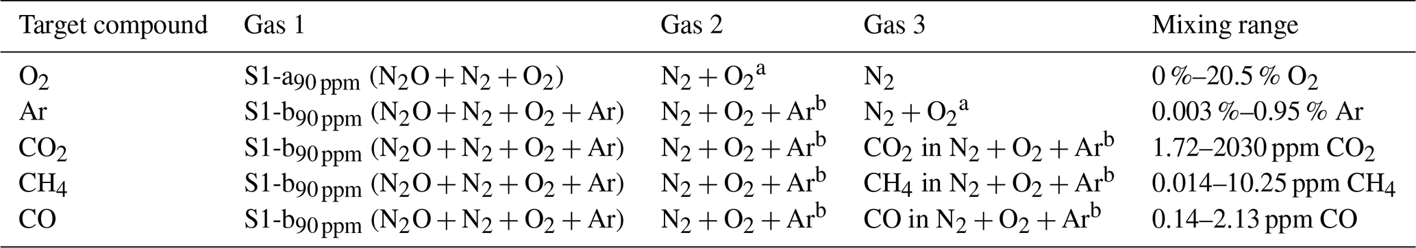
a Matrix a: 20.5 % O2 in N2. b Matrix b: 20.95 % O2, 0.95 % Ar in N2.
2.4.6 Trace gas effects (CO2, CH4, CO and H2O)
The sensitivity of [N2O] and δ values on changing trace gas concentrations was tested in a similar way to those described in Sect. 2.4.5. In short, Gas 1 (S1-b90 ppm) was dynamically diluted with Gas 2 (matrix b) to create an Anchor gas with 330 ppb N2O in matrix b. Gases 1, 2 and 3 (either CO2, CH4 or CO in matrix gas b) were mixed to incrementally change the mixing ratios of the target substances (1.7–2030 ppm CO2, 0.01–10.25 ppm CH4 and 0.14–2.14 ppm CO) while maintaining a consistent gas matrix and [N2O] of 330 ppb (Table 5). Trace gas mole fractions in the produced gas mixtures were analyzed with a Picarro G2401 (Picarro Inc., USA) and agreed with predictions within better than 2 %–3 % (relative). Similar to Sect. 2.4.4, the effects of increasing CO2, CH4 and CO on [N2O] and δ values were quantified by comparing the measured [N2O] and δ values at each step change to the mean measured [N2O] and δ values of the Anchor gas and were denoted Δ[N2O] and Δδ. Similar to Sect. 2.4.5, deviations in CO2 CH4 and CO mixing ratios were quantified by comparing the measured [CO2], [CH4] and [CO] at each step change to the mean measured [CO2], [CH4] and [CO] of the Anchor gas. Each experiment was triplicated. The interference effects were also tested at ∼660 ppb and ∼990 ppb N2O.
The sensitivity of the analyzers to water vapor was tested by firstly diluting Gas 1 (S1-c90 ppm) with Gas 2 (matrix c) to produce an Anchor gas with 330 ppb N2O. This mixture was then combined with Gas 3 (also matrix c) which had been passed through a humidifier (customized setup by Glasbläserei Möller, Switzerland) set to 15 ∘C (F20 Julabo GmbH, Germany) dew point. By varying the flows of Gases 2 and 3, different mixing ratios of water vapor ranging from 0 to 13 800 ppm were produced and measured using a dew-point meter (model 973, MBW, Switzerland). H2O effects were quantified as described above, but [N2O] results were additionally corrected for dilution effects caused by the addition of water vapor into the gas stream. Water vapor dependence testing was not performed on the TREX-QCLAS I, as the instrument is equipped with a permeation dryer at the inlet.
2.4.7 CO2 and CO removal using NaOH (Ascarite) and Sofnocat
The efficiency of NaOH and Sofnocat for removing spectral effects caused by CO2 and CO was assessed by repeating CO2 and CO interference tests (Sect. 2.4.6) but with the respective traps connected in line. These experiments were triplicated but only undertaken at ∼330 ppb N2O. NaOH traps were prepared using stainless steel tubing (OD 2.54 cm, length 20 cm) filled with 14 g Ascarite (0–30 mesh, Sigma Aldrich, Switzerland) bracketed by 3 g Mg(ClO4)2 (Alfa Aesar, Germany) each separated by glass wool. The Sofnocat trap was prepared similarly using stainless steel tubing (OD 2.54 cm, length 20 cm) filled with 50 g Sofnocat (Sofnocat 423, Molecular Products Limited, GB) and capped on each side with glass wool.
2.4.8 Two-end-member mixing
The ability of the instruments to accurately extrapolate N2O source compositions was tested using a simulated two-end-member mixing scenario in which a gas with high N2O concentration, considered to be a N2O source gas (SG), was dynamically diluted into a gas with ambient N2O concentration (PA2), considered to be background air. N2O mole fractions were raised above ambient levels (denoted as ΔN2O) in three different scenarios ranging (1) 0–30 ppb, (2) 0–700 ppb and (3) 0–10 000 ppb. In each scenario, two isotopically different source gases with high N2O concentration were used; one source gas (SG1-a90 ppm) was 15N depleted compared to PA2, and a second source gas (SG2-a90 ppm) was 15N enriched compared to PA2 (Table 3). The three different mixing scenarios and two different source gases resulted in a total of six mixing scenarios (referred to as Exps. 1–6). During each experiment, PA2 was alternated with PA2+SG in four different mixing ratios to give a span of N2O concentrations and isotopic compositions required for Keeling plot analysis. Each experiment was triplicated. OA-ICOS I and QCLAS I were used in all experiments (Exps. 1–6), CRDS was used for ΔN2O 0–30 ppb and 0–700 ppb (Exps. 1–4) and TREX-QCLAS was only used for ΔN2O 0–30 ppb (Exps. 1–2).
To test the robustness of trace gas correction equations derived for each analyzer in Sect. 3.6, NaOH and Sofnocat traps were placed in line between the PA2+SG mixtures and the analyzers such that we could ensure a difference in CO2 and CO mole fractions between the measured gas mixture and reference gases (S1-c330 ppb, S2-c330 ppb). The experiments were also bracketed by two calibration phases (S1-c330 ppb, S2-c330 ppb) to allow for δ calibration, followed by two phases where the N2O concentration dependence was determined.
Gas samples for GC-IRMS analysis were taken in the same phase (last 5 min of 15 min interval) used during the minute prior to the final 5 min used for averaging by the laser-based analyzers. The gas was collected at the common overflow port of the laser spectrometers using a 60 mL syringe connected via a Luer lock three-way valve to the needle and port. The 200 mL samples were taken at each concentration step. A 180 mL gas sample was stored in pre-evacuated 110 mL serum crimp vials for isotopic analysis using IRMS. IRMS analyses were conducted at ETH Zürich using a gas preparation unit (Trace Gas, Elementar, Manchester, UK) coupled to an IsoPrime100 IRMS (Elementar, Manchester, UK). The remaining 20 mL were injected in a pre-evacuated 12 mL Labco exetainer for [N2O] analysis using gas chromatography equipped with an electron capture detector (ECD) performed at ETH Zürich (Bruker, 456-GC, Scion Instruments, Livingston, UK). After injection, samples were separated on HayeSep D packed columns with a 5 % CH4 in Ar mixture (P5) as carrier and make-up gas. The GC was calibrated using a suite of calibration gases at N2O concentrations of 0.393 (Carbagas AG, Switzerland), 1.02 (PanGas AG, Switzerland) and 3.17 ppm (Carbagas AG, Switzerland). For further analytical details, see Verhoeven et al. (2019) and Sect. S1.
For the laser-based analyzers, data were processed as described in Sect. 2.3.2 using the following sequential order: (1) analyzer-specific correction functions, determined in Sect. 3.6, were applied to correct for differences in trace gas concentrations (CO2, CO) between sample gas and calibration gases; (2) the effect of [N2O] changes was corrected using a three-point correction; (3) a drift correction based on repeated measurements of PA2 was applied if necessary; and (4) δ values standardized to international scales (Eq. 4) using S1-c330 ppb and S2-c330 ppb.
Note that due to the large number of results acquired in this section, only selected results are shown in Figs. 3 to 14. The complete datasets (including [N2O], δ15Nα, δ15Nβ and δ18O acquired by all instruments tested) are provided in Sect. S4.
3.1 Allan precision
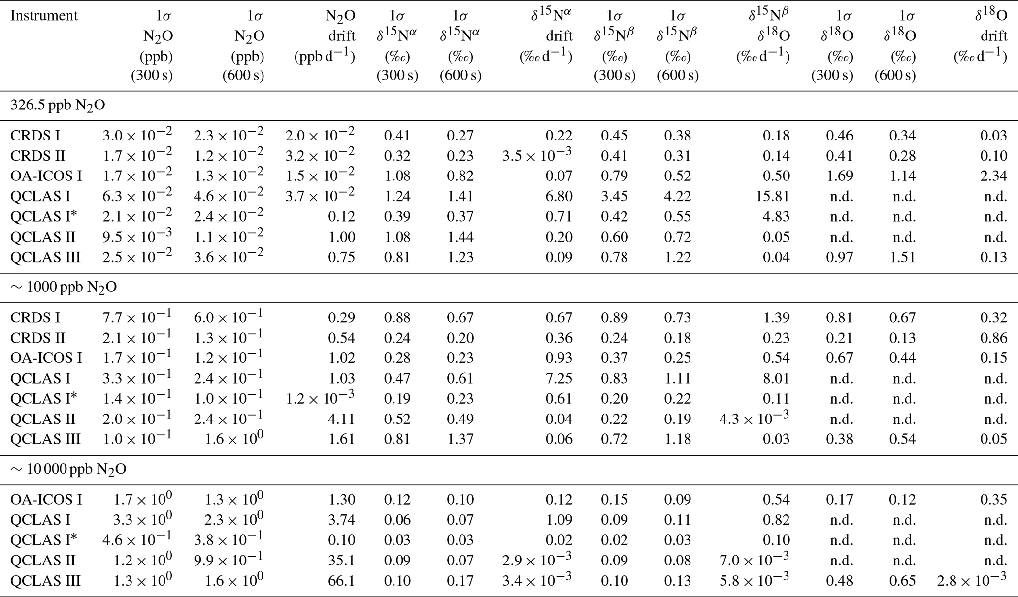
Allan deviations (square root of Allan variance) for 5 and 10 min averaging times, often reported in manufacturer specifications, at ∼327, 1000 and 10 000 ppb [N2O] are shown in Table 6.
At near-atmospheric N2O mole fractions of ∼326.5 ppb, both CRDS analyzers showed the best precision and stability for the measurement of δ15Nα, δ15Nβ and δ18O (0.32 ‰–0.41 ‰, 0.41 ‰–0.45 ‰, 0.41 ‰–0.46 ‰ at 300 s averaging time, respectively), while for the precision of [N2O], the OA-ICOS I and the CRDS II showed best performance ( ppb at 300 s averaging time) (Figs. 3 and S4-1; Table 6). The Allan precision of CRDS and OA-ICOS analyzers further improved with increasing averaging times, and optimal averaging times typically exceeded 1.5–3 h. The precision and daily drift of the OA-ICOS I and both CRDS analyzers were in agreement with manufacturer specifications (ABB – Los Gatos Research Inc., 2019; Picarro Inc., 2019). The CRDS II outperformed the CRDS I for precision, presumably due to manufacturer upgrades/improvements in the newer model. The QCLAS spectrometers exhibited significant differences between instruments, which might be due to differences in the instrument hardware/design, as instruments were manufactured between 2012 and 2016, or in the parameter setting (such as cell pressure and tuning parameters) of different analyzers.
Generally, short-term (approximately up to 100 s) precision of QCLAS instruments was compatible or superior to CRDS or OA-ICOS, but data quality was decreased for longer averaging times due to drift effects. Nonetheless, the performance of QCLAS I, II and III generally agrees with Allan precision measurements executed by Yamamoto et al. (2014), who reported 1.9 ‰–2.6 ‰ precision for δ values at ambient N2O mole fractions and 0.4 ‰–0.7 ‰ at 1000 ppb N2O. QCLAS I, which was tested further in Sect. 3.2–3.7, displayed the poorest performance of all QCLAS analyzers, in particular for δ15Nβ. The primary cause of the observed excess drift in QCLAS I was fluctuating spectral baseline structure (ARI, personal communication, 2019), which can be significantly reduced by applying an automatic spectral correction method developed by ARI. This methodology is currently in a trial phase and thus not yet implemented in the software that controls the QCLAS instruments. A brief overview of the methodology is provided in Sect. S5, and corrected results for QCLAS I are provided in Table 6. This methodology is not discussed in detail here as it is beyond the scope of this work. Nonetheless, QCLAS I achieved Allan deviations of ∼0.4 ‰ at 300 s averaging time for δ15Nα and δ15Nβ at ambient N2O mole fractions when this correction method was applied by ARI.
At [N2O] of 1000 ppb, the precision of δ values measured by all analyzers, except CRDS I, significantly improved due to greater signal-to-noise ratios. Whilst the performance of OA-ICOS I was similar to that of CRDS II for δ15Nα and δ15Nβ (0.24 ‰ and 0.24 ‰ for CRDS II; 0.28 ‰ and 0.37 ‰ for OA-ICOS I at 300 s averaging time), CRDS II displayed the best precision for δ18O (0.21 ‰ at 300 s averaging time). Also notable was the improved performance of the 2018 model (CRDS II) compared to the 2015 model (CRDS I). QCLAS analyzers showed the best 1 s precision for δ values, but beyond 100 s, δ measurements were still heavily affected by instrumental drift resulting in lower precision, especially for QCLAS I. When the spectral correction method described in Sect. S5 was applied, QCLAS I achieved Allan deviations of ∼0.2 ‰ at 300 s averaging time for δ15Nα and δ15Nβ at 1000 ppb N2O.
At [N2O] of 10 000 ppb, all analyzers showed excellent precision, with QCLAS I, II and III outperforming OA-ICOS I for precision of δ15Nα and δ15Nβ (collectively better than 0.10 ‰ at 300 s averaging time for both δ15Nα and δ15Nβ). QCLAS II had the best precision for [N2O] (1.2 ppb at 300 s averaging time). OA-ICOS I and QCLAS III were the only analyzers tested in this study that could be used to measure δ18O at 10 000 ppb N2O. OA-ICOS I attained a precision of 0.17 ‰, while QCLAS III attained a precision of 0.48 ‰, both with 300 s averaging time. QCLAS I achieved Allan deviations of ∼0.02 ‰–0.03 ‰ at 300 s averaging time for δ15Nα and δ15Nβ at 10 000 ppb N2O when the spectral correction method (Sect. S5) was applied.
The precision of instruments on [N2O] measurements at 1000 and 10 000 ppb N2O might not be representative because of small fluctuations in the final gas mixture produced by the MFCs, which were likely amplified due to the small dilution ratios. Moreover, the different relative increases in Allan deviation compared to measurements at 326.5 ppb might have been caused by the different internal plumbing volumes, flow rates and spectral fits used for the analyzers, which could scale or add to the increased Allan deviation introduced via the MFCs. Therefore, the indicated [N2O] precisions should be considered as a pessimistic estimate. Nonetheless, the observed decline in [N2O] precision for all analyzers was around 1 order of magnitude when changing from atmospheric N2O mole fractions to 1000 ppb N2O and from 1000 ppb to 10 000 ppb N2O.
Table 6Key parameters for instrument stability retrieved from Allan variance experiments for [N2O], δ15Nα, δ15Nβ and δ18O: precision (1σ) at 300 and 600 s averaging times, and daily drift at various N2O concentrations. The 1σ data refer to Allan deviation (square root of Allan variance).
* Data were reprocessed by Aerodyne Research Inc. technicians using an
automatic spectral correction method. This method corrects data that were
influenced by changing baseline structure.
Further information on this
method is provided in Sect. S5.
“n.d.” indicates not determined.
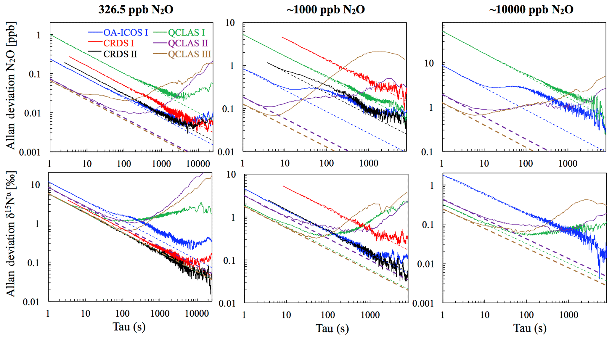
Figure 3Allan deviation (square root of Allan variance) plots for the OA-ICOS I (blue), CRDS I (red), CRDS II (black), QCLAS I (green), QCLAS II (purple) and QCLAS III (brown) at different N2O mole fractions (∼327, 1000 and 10 000 ppb). The dashed lines represent a slope of −0.5 (log–log scale) and indicate the expected behavior for Gaussian white noise in each analyzer. The Allan deviations of all analyzers tested were reproducible on three separate occasions prior to the test results presented here. Allan deviation plots for δ15Nβ and δ18O are provided in Sect. S4 (Fig. S4-1 in the Supplement).
3.2 Temperature effects
All instruments tested showed significant effects, albeit to varying degrees, on their measurements due to the change in laboratory temperature (Figs. 4 and S4-2). The OA-ICOS I displayed no clear temperature effects for [N2O], δ15Nα and δ15Nβ but displayed a moderate temperature dependence for δ18O measurements (up to 14 ‰ deviation from the mean), with measurement drift closely paralleling the laboratory temperature (r2=0.78). Both CRDS instruments displayed smaller shifts in [N2O] (up to 0.14 ppb deviation from the mean), δ15Nα, δ15Nβ and δ18O that occurred particularly when the laboratory temperature had an acute change. QCLAS I showed a strong temperature dependence on δ15Nα (r2=0.85) and δ15Nβ (r2=0.96).
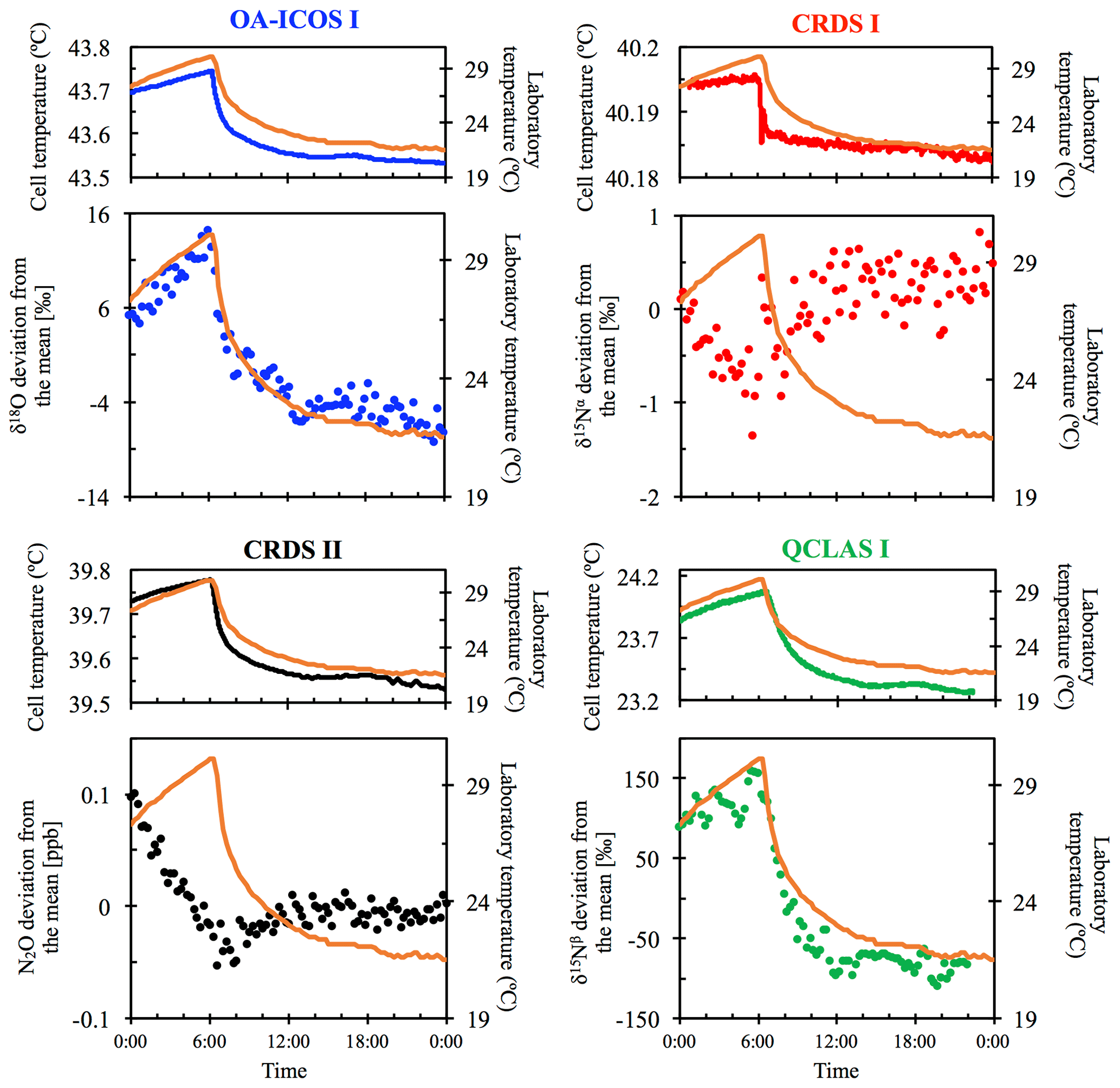
Figure 4Examples of the dependency of different measurements on laboratory temperature (∘C) for OA-ICOS I (blue), CRDS I (red), CRDS II (black) and QCLAS I (green). The complete dataset is provided in Sect. S4 (Fig. S4-2). The laboratory temperature is indicated by a solid orange line and was allowed to vary over time. Cell temperatures for each instrument are also plotted for comparison. The analyzers began acquiring measurements at 00:00 CEST on 8 July 2018, capturing the end of the rising limb of the laboratory temperature. Results are plotted as the deviation from the mean, without any anchoring to reference gases.
3.3 Repeatability
The best long-term repeatability for δ values was achieved by TREX-QCLAS I with 0.60 ‰ for δ15Nα, 0.37 ‰ for δ15Nβ and 0.46 ‰ for δ18O, even though measurements were taken over a 6-month period (Table 7). The best repeatability without preconcentration was achieved by CRDS analyzers with 0.52 ‰–0.75 ‰ for CRDS II and 0.79 ‰–0.83 ‰ for CRDS I for all δ values. OA-ICOS I achieved repeatability between 1 ‰–2 ‰ (1.47 ‰, 1.19 ‰ and 2.17 ‰ for δ15Nα, δ15Nβ and δ18O, respectively). QCLAS I isotopic measurements attained repeatability of 5.4 ‰ and 8.6 ‰ for δ15Nα and δ15Nβ, respectively. Short-term repeatability results for 10 repeated 15 min measurements periods over 2.5 h are provided in Sect. S6.
Table 7Summary of the measured [N2O], δ15Nα, δ15Nβ and δ18O and associated 1σ at 300 s averaging times based on repeated measurements of PA1.

3.4 Dependence of isotopic measurements on N2O mole fraction
There was an offset in measured δ values resulting from the change in [N2O] introduced to the analyzers (Figs. 5 and S4-3). A linear relationship between Δδ15Nα, β and Δδ18O values with [1∕N2O] was observed across all analyzers. However, examination of the residuals from the linear regression revealed varying degrees of residual curvature, highlighting that further non-linear terms would be required to adequately describe, and correct for, this mole fraction dependence. Repeated analysis of [N2O] dependencies on consecutive days showed similar trends, indicating that the structure of non-linear effects might be stable over short periods of time. Nevertheless, there were small variabilities in δ values at a given N2O mole fraction, which could be due to the inherent uncertainty of the measurement and/or day-to-day variations in the mole fraction dependence. The standard deviation of individual 5 min averages of δ15Nα, β and δ18O also varied according to the [N2O] measured by each analyzer due to variations in the signal-to-noise ratio (Sect. S7).
Figure 5Deviations of the measured δ15Nα, δ15Nβ and δ18O values according to 1∕[N2O] for the OA-ICOS I (blue), CRDS I (red), CRDS II (black) and QCLAS I (green). Measurements span the manufacturer-specified operational ranges of the analyzers. The experiment was repeated on three separate days. A linear regression is indicated by the solid line, and a residual plot is provided above each plot. Individual linear equations, coefficients of determination (r2) and p values are indicated above each plot. The remaining plots for δ15Nβ and δ18O are provided in Sect. S4 (Fig. S4-3).
3.5 Gas matrix effects (O2 and Ar)
3.5.1 Gas matrix effects at ambient N2O mole fractions
With the exception of TREX-QCLAS I, all instruments displayed strong O2 dependencies for [N2O] and δ values (Figs. 6 and S4-4). For these instruments, linear regressions best described the offset of measured [N2O] and δ values resulting from the change in O2 composition of the matrix gas. Importantly, CRDS I and II displayed different degrees of O2 interference on [N2O] and δ values, suggesting that these dependencies were either analyzer-specific or differences were due to hardware/software modifications between different production years. Preconcentration prior to analysis, as performed in TREX–QCLAS I, eliminated O2 dependencies as the gas matrix was normalized to synthetic air (20.5 % O2).
The change in Ar composition of the matrix gas caused minor, yet measurable, interferences on [N2O] and δ measurements (Fig. S4-5). The range investigated was between approximately 0 % and 0.95 % Ar, as anticipated for N2O in synthetic air (no Ar) reference gas versus a whole air (with Ar) sample gas. The effects observed for a 0.95 % change in [Ar] were significantly smaller than that observed for O2 but might extend to a similar range for sample and reference gases with higher differences in [Ar]. The interference effects were found to be best described by second-order polynomial functions, though we expect that a linear fit would serve equally well if a larger change in [Ar] was investigated. Although most functions to describe the dependence on Ar across all instruments were statistically significant (p<0.05), maximum effects did not transgress the repeatability (1σ) of the Anchor gas measurements. TREX-QCLAS I measurements were not impaired by gas matrix effects.

Figure 6Deviations of the measured [N2O], δ15Nα, δ15Nβ and δ18O values according to ΔO2 (%) at different N2O mole fractions (330, 660 and 990 ppb) for the OA-ICOS I (blue), CRDS I (red), CRDS II (black), QCLAS I (green) and TREX-QCLAS I (brown). The remaining plots for [N2O], δ15Nα and δ18O are provided in Sect. S4 (Fig. S4-4). The standard deviation of the Anchor gas (±1σ) is indicated by dashed lines. Data points represent the mean and standard deviation (1σ) of triplicate measurements. Dependencies are best described using linear regressions, which are indicated by a solid line. Individual equations, coefficients of determination (r2) and p values are indicated above each plot for the 330 ppb N2O data only.
3.5.2 Continuity of gas matrix corrections at higher N2O mole fractions
When mole fractions of 660 and 990 ppb N2O were measured by the laser spectrometers, O2 interference effects on [N2O] and δ values were well described using linear regression, albeit with different slopes to those obtained for 330 ppb N2O (Figs. 6 and S4-4; Sect. S8).
We could not adequately predict the nature in which the slopes of the interference effects scaled with N2O mole fractions. Overall, this suggests that interference effects were analyzer-specific and varied according to instrument-specific parameters, rather than due to bona fide scaling of the pressure-broadening effect. Therefore, to account for combined effects of [O2] and [N2O] changes on measurements, a user would be required to perform a series of laboratory tests across the range of expected [O2] and [N2O]. In an exemplary approach, we applied a series of empirical equations (Eqs. 5–6) to predict the offset of measured [N2O] and δ values caused by changes in [O2] as a function of [N2O] introduced to the analyzers in this study:
where and Δδmeas, mix are the measured offsets on [N2O] and δ values for the gas mixtures introduced to the analyzers as reported in Sect. 3.5.1, respectively; is the difference in O2 mole fraction between the gas mixture and Anchor gas as reported in Sect. 3.5.1; is the expected [N2O] of gas mixtures introduced to the analyzer, calculated based on gas flows and cylinder compositions of Gases 1, 2 and 3 as reported in Sect. 2.4.5; A and B, and a, b and c are analyzer-specific constants.
Using Eqs. (5) and (6) to fit values for the constants A and B for , and a, b and c for Δδmeas, mix resulted in a total of 11 analyzer-specific values (Sect. S8). With gas-specific constants established, interferences on [N2O] and δ measurements for a sample gas G for a given analyzer can be corrected using Eqs. (7)–(8):
where [N2O]mc, G and δmc, G are the matrix-corrected [N2O] and δ values of sample gas G, respectively; Δ[O2]G is the difference in O2 mole fraction between sample gas G and reference gases. Correction using Eqs. (7)–(8) removes the O2 effect to a degree that corrected measurements from Sect. 3.5.1 are typically within the uncertainty bounds of the anchor (Sect. S8).
Although Ar effects seemingly scaled with increased N2O mole fractions, we did not derive scaling coefficients for Ar because the derived Ar correction equations at 330, 660 and 990 ppb N2O were typically not statistically significant at p<0.05. These interferences also did not always exceed the repeatability of Anchor gas measurements. Although we could have tested for effects for [Ar] changes greater than 0.95 %, we limited our experiments to [Ar] expected in tropospheric samples.
3.6 Trace gas effects (H2O, CO2, CH4 and CO)
3.6.1 Trace gas effects at ambient N2O mole fractions
The apparent offset of [N2O] and δ values resulting from the change in CO2 composition of the matrix gas was best described by linear functions (Figs. 7 and S4-6). OA-ICOS I exhibited discrete and well-defined linear interference effects of CO2 on [N2O], δ15Nα, δ15Nβ and δ18O (all r2>0.95), likely due to crosstalk between CO2 absorption lines situated near 2192.46 and 2192.33 cm−1. Both CRDS instruments showed CO2 interference effects of smaller magnitude for [N2O], δ15Nα and δ18O, presumably due to CO2 absorption lines at 2196.21, 2195.72 and 2196.02 cm−1. QCLAS I displayed less well-defined CO2 interference effects for δ15Nβ, which was possibly due to several overlapping absorption lines of CO2 located near 2187.85 cm−1. All linear functions derived for the TREX-QCLAS I were not statistically significant at p<0.05. As shown in Figs. 7 and S4-6, the NaOH trap was effective in removing the CO2 effect (if present) across the mole fraction ranges tested for all instruments.
Similarly, CH4 effects on apparent [N2O] and δ values were well described by linear functions (Figs. 8 and S4-7). The largest effects were for CRDS I and II, which both displayed strong CH4 dependencies for δ15Nα and δ18O of similar magnitude. This might be due to crosstalk of 14N15N16O and 14N14N18O absorption lines with the respective CH4 lines located at 2195.76 and 2195.95 cm−1. For OA-ICOS I, minor CH4 effects were observed for δ15Nβ, due to absorption line overlap at 2192.33 cm−1. QCLAS I did not display any CH4 interference effect over the tested [CH4] range. Linear functions derived for the TREX-QCLAS I were not statistically significant at p<0.05. The similarity between the [N2O] dependencies on CH4 mole fractions for OA-ICOS I, CRDS I, II and QCLAS I suggests that the apparent effects may be due to small fluctuations in the gas mixtures produced by the MFCs, rather than a discrete spectral interference effect.
The CRDS analyzers showed minor interference effects for δ15Nα and δ15Nβ on [CO] (0.14–2.14 ppm) (Fig. S4-8), likely due to crosstalk with CO absorption lines located at 2195.69 and 2195.83 cm−1. The magnitude of these effects was similar for both models. QCLAS I displayed interference effects for δ15Nα and δ15Nβ caused by a CO absorption line located near 2187.9 cm−1, although this effect did not exceed the repeatability of the Anchor gas (containing no CO) over the measurement range. The effects of [CO] on δ values acquired using OA-ICOS I and TREX-QCLAS I were not statistically significant at p<0.05. Similar to CH4, the resemblance of [CO] effects to [N2O] measurements for OA-ICOS I, CRDS I, II and QCLAS I suggests that the apparent effects may be due to inaccuracies in the dynamic dilution process, rather than a discrete spectral interference effect. The Sofnocat trap was effective in removing CO (if present) across the mole fraction ranges tested for all instruments.
OA-ICOS I exhibited large effects of [H2O] (0–13 800 ppm) on δ15Nβ (up to −10 ‰) and δ18O (up to −15 ‰), and minor dependencies for δ15Nα (up to 4 ‰) and [N2O] (up to 1 ppb) across the range tested (Fig. S4-9). For QCLAS I, the H2O effect was largest for δ15Nα (up to 20 ‰), whilst minor effects for [N2O] (up to 2 ppb) were observed in relation to the Anchor gas (no H2O). In contrast, both CRDS instruments showed no significant effects across the range tested, which is attributable to the installation of permeation dryers inside the analyzers by the manufacturer.
Figure 7Deviations of the measured [N2O], δ15Nα, δ15Nβ and δ18O values according to ΔCO2 (ppm) at different N2O mole fractions (330, 660 and 990 ppb) for the OA-ICOS I (blue), CRDS I (red), CRDS II (black), QCLAS I (green) and TREX-QCLAS I (brown). The remaining plots for [N2O], δ15Nα and δ18O are provided in Sect. S4 (Fig. S4-6). The standard deviation of the Anchor gas (±1σ) is indicated by dashed lines. Data points represent the mean and standard deviation (1σ) of triplicate measurements. Dependencies are best described by linear fits, which are indicated by solid lines. Individual equations, coefficients of determination (r2) and p values are indicated above each plot for the 330 ppb N2O data only.
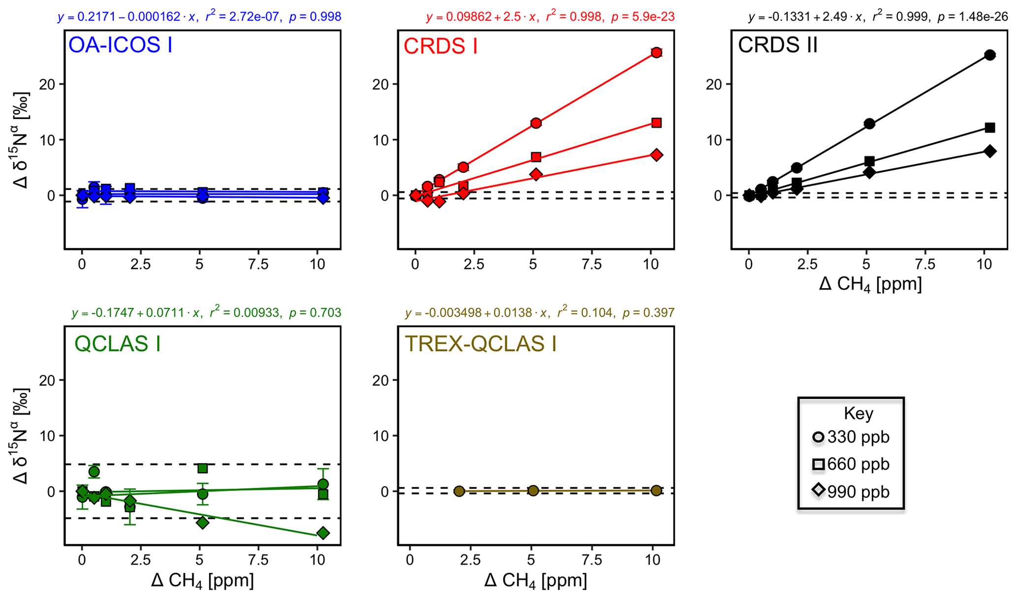
Figure 8Deviations of the measured [N2O], δ15Nα, δ15Nβ and δ18O values according to ΔCH4 (ppm) at different N2O mole fractions (330, 660 and 990 ppb) for the OA-ICOS I (blue), CRDS I (red), CRDS II (black), QCLAS I (green) and TREX-QCLAS I (brown). The remaining plots for [N2O], δ15Nβ and δ18O are provided in Sect. S4 (Fig. S4-7). Data points represent the mean and standard deviation (1σ) of triplicate measurements. Dependencies are best described by linear fits, which are indicated by solid lines. Individual equations, coefficients of determination (r2) and p values are indicated above each plot for the 330 ppb N2O data only.
3.6.2 Continuity of trace gas corrections at higher N2O mole fractions
Interference effects from CO2, CH4 and CO on apparent δ values, where significant, inversely scaled with increasing [N2O] (Figs. 7, 8, S4-8 and Sect. S8). The scaling of trace gas effects can be explained by simple spectral overlap of the 14N15N16O, 15N14N16O and 14N14N18O lines with those of the trace gas, which results in the interference effects being inversely proportional to the mixing ratio of N2O. However, there may be additional spectral overlap between the trace gas and the 14N14N16O peak resulting in an offset for the measured [N2O], which introduces a further shift in the δ values (as shown in Sect. 3.4). The effect on the apparent [N2O] was less clear and was possibly confounded by inaccuracies during dynamic gas mixing. In this study, the scaling of interference effects from trace gases as a function of the [N2O] introduced to the analyzers could be described using Eqs. (9) and (10):
where Δ[N2O]meas, mix and Δδmeas, mix are the measured offsets on [N2O] and δ values for the gas mixtures introduced to the analyzers as reported in Sect. 3.6.1, respectively; Δ[x]A is the difference in trace gas mole fraction between the gas mixture and Anchor gas as reported in Sect. 3.6.1; and Ax, Bx, ax and bx are constants that are trace gas and instrument specific. The constant bx only occurs when there is spectral overlap from the trace gas and 14N14N16O absorption lines.
For a sample gas G, the effect can then be corrected by using Eqs. (11) and (12):
In Eqs. (11)–(12), the sum of the effect of all interfering gases with overlapping absorption lines is taken into account. Similar to Sect. 3.5.2, correction using Eqs. (11)–(12) removes the trace gas interference effects to the extent that corrected measurements from Sect. 3.6.1 are within the repeatability bounds of the Anchor gas (Sect. S8). Similar inverse relationships have been described by Malowany et al. (2015) for H2S interferences on δ13C−CO2.
3.7 Two-end-member mixing
Results for the two-end-member mixing experiment were evaluated in two different ways. First, results for individual gas mixtures acquired by laser spectroscopy and GC-IRMS were compared to expected [N2O] and δ values calculated from N2O mole fractions and isotopic composition of end-members and mixing fractions. Second, source values were extrapolated using a weighted total least squares regression analysis, known as Keeling plot analysis (Keeling, 1958), and compared to assigned δ values of the source gas used in each experiment.
3.7.1 Comparison with expected [N2O] and δ values
Triplicate measurements (mean ±1σ) obtained using the laser spectrometers and GC-IRMS were plotted against expected [N2O] and δ values calculated using MFC flow rates, N2O mole fractions and isotopic composition of background and source gases (Figs. 12–15). Comparisons between individual laser spectrometer measurements and GC-IRMS are plotted in Sect. S9 and are discussed only briefly below.
OA-ICOS I
Generally, there was good agreement of [N2O] between the OA-ICOS I and expected values, although the analyzer overestimated mole fractions at higher ΔN2O during Exps. 5 and 6. There was excellent agreement between the OA-ICOS I and calculated expected δ values (all r2>0.95; Figs. 9 and S4-10). Measurements for δ15Nα were mostly within ±2.4 ‰ of expected values, while δ15Nβ, δ15Nbulk and SP were all within ±2 ‰ of expected values. δ18O measurements were the poorest performing but were typically within ±3.6 ‰ of expected values. Similarly, there was excellent agreement between OA-ICOS I and IRMS isotope values (all r2>0.95), which agreed within 1.7 ‰–2.4 ‰ (Fig. S9-2). The standard deviations of triplicate isotope measurements decreased dramatically with increasing ΔN2O, improving from 1 ‰ to 2 ‰ during Exps. 1 and 2 to typically better than 0.1 ‰ during Exps. 5 and 6. Conversely, the standard deviations of triplicate sample measurements for [N2O] increased with increasing ΔN2O, rising from <0.1 ppb during Exps. 1–4 to >1 ppb during Exps. 5 and 6. Nonetheless, all OA-ICOS I [N2O] measurements had better 1σ repeatability than those acquired using GC. The repeatability of the triplicate isotope measurements with OA-ICOS I was typically better than IRMS exclusively at higher ΔN2O (>700 ppb).
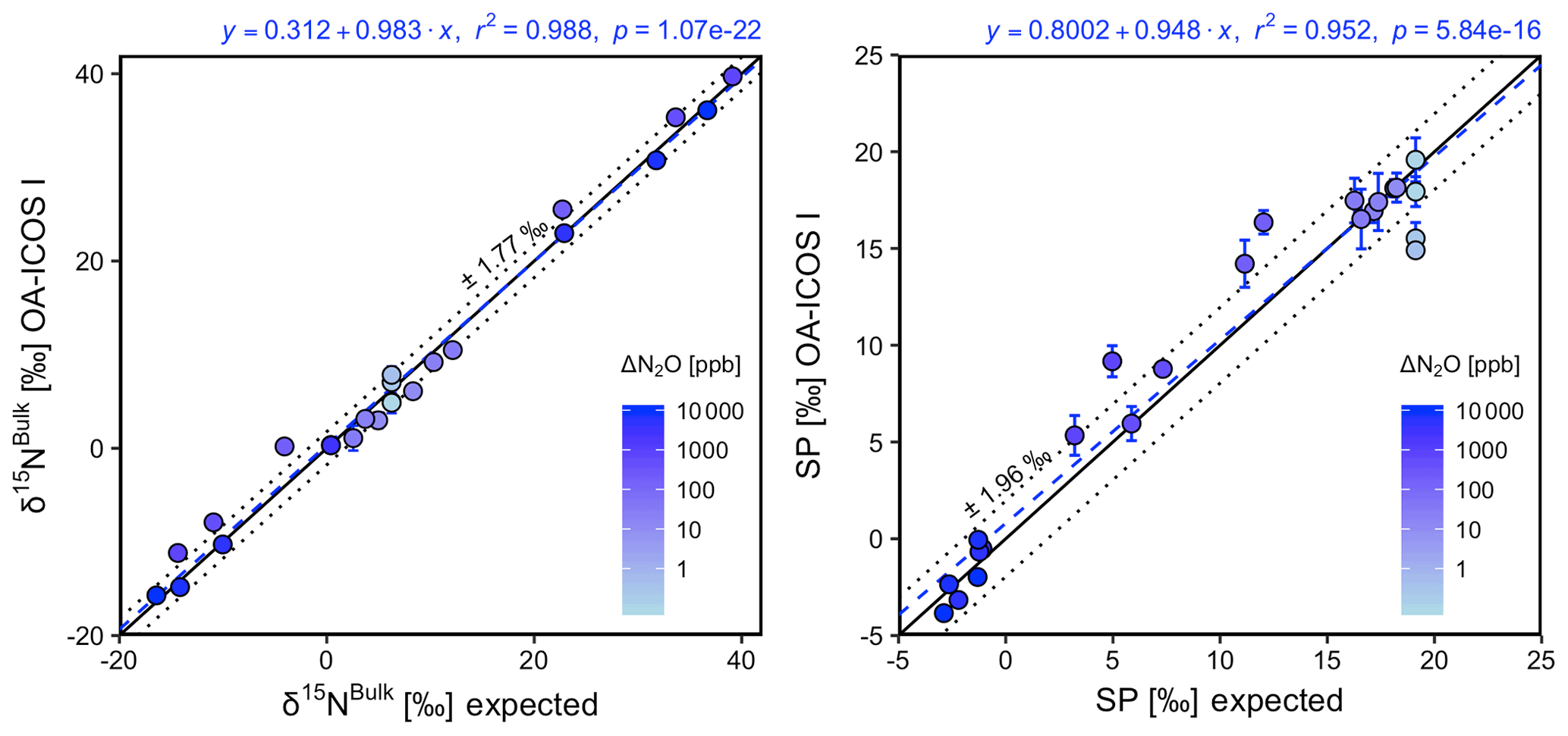
Figure 9Correlation diagrams for δ15Nbulk and SP measurements at various ΔN2O mole fractions analyzed by OA-ICOS I plotted against expected values. The remaining plots for [N2O], δ15Nα, δ15Nβ and δ18O are provided in Sect. S4 (Fig. S4-10). The solid black line denotes the 1:1 line, while the dotted line indicates ±1σ of the residuals from the 1:1 line. The dashed blue line represents a linear fit to the data. Individual equations, coefficients of determination (r2) and p values are indicated above each plot. Each data point represents the mean and standard deviation (1σ) of triplicate measurements. The inset plots indicate the standard deviation (1σ) of the triplicate measurements achieved at different ΔN2O mole fractions, and the 1:1 line is similarly a solid line.
CRDS I
[N2O] acquired by CRDS I were in good agreement with expected values, although the analyzer slightly underestimated mole fractions at higher ΔN2O during Exps. 3 and 4. There was excellent agreement between the CRDS I and calculated expected isotope values (all r2>0.95; Figs. 10 and S4-11). Measurements for δ15Nα and δ15Nβ were mostly better than ±1.1 ‰ of expected values, while δ15Nbulk was within ±0.5 ‰ of expected values. SP and δ18O measurements were typically within ±1.5 ‰ of expected values. There was excellent agreement between CRDS I and IRMS isotope values (all r2>0.93), which agreed to within 0.5 ‰–1.9 ‰ (Fig. S9-3). In general, the standard deviations of triplicate isotope measurements increased as a function of ΔN2O, with the lowest deviations of 0.1 ‰–1 ‰ occurring when ΔN2O<100 ppb. However, two triplicated measurements for δ15Nbulk had standard deviations better than 0.1 ‰. The standard deviations of triplicate measurements for [N2O] also increased with increasing ΔN2O mole fractions, rising from 0.03–0.07 ppb when ppb (i.e., ambient conditions) to ∼1 ppb when ppb. With the exception of one triplicate measurement, all CRDS I [N2O] measurements had better 1σ repeatability than those acquired using GC. Overall, IRMS had slightly better repeatability (most ranging from 0.1 ‰ to 1 ‰) than CRDS I (most ranging from 0.1 ‰ to 2 ‰) for isotopic measurements.
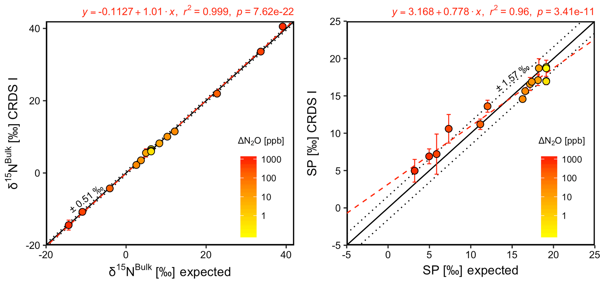
Figure 10Correlation diagrams for δ15Nbulk and SP measurements at various ΔN2O mole fractions analyzed by CRDS I plotted against expected values. The remaining plots for [N2O], δ15Nα, δ15Nβ and δ18O are provided in Sect. S4 (Fig. S4-11). The solid black line denotes the 1:1 line, while the dotted line indicates ±1σ of the residuals from the 1:1 line. The dashed red line represents a linear fit to the data. Individual equations, coefficients of determination (r2) and p values are indicated above each plot. Each data point represents the mean and standard deviation (1σ) of triplicate measurements. The inset plots indicate the standard deviation (1σ) of the triplicate measurements achieved at different ΔN2O mole fractions, and the 1:1 line is similarly a solid line.
CRDS II
Similar to results for CRDS I, [N2O] acquired by CRDS II were in good agreement with expected values but slightly underestimated mole fractions at higher ΔN2O during Exps. 3 and 4. There was excellent agreement between the CRDS II and calculated expected isotope values (all r2>0.99; Figs. 11 and S4-12). Measurements for δ15Nα and SP were typically better than ±0.8 ‰ of expected values, while δ15Nβ, δ15Nbulk measurements were all within ±0.4 ‰ of expected values. δ18O measurements were within ±1.0 ‰ of expected values. There was excellent agreement between CRDS II and IRMS isotope values (all r2>0.98), which agreed within ±0.6 ‰–1.4 ‰ (Fig. S9-4). The standard deviations of triplicate isotope measurements typically decreased as a function of ΔN2O, with the lowest deviations of <0.1 ‰–0.3 ‰ occurring when ppb. Conversely, the standard deviations of triplicate sample measurements for [N2O] increased with increasing ΔN2O, rising from 0.04–0.09 ppb when ppb (i.e., ambient conditions) to ∼0.4 ppb when ppb. All CRDS II [N2O] measurements had better 1σ repeatability than those acquired using GC. There was no clear distinction between CRDS II and IRMS triplicate repeatability, with both achieving triplicate repeatability ranging from 0.1 ‰ to 1 ‰ for most isotopic measurements. However, the repeatability of SP CRDS II measurements was mostly better than IRMS, achieving triplicate repeatability between 0.1 ‰ and 0.6 ‰, compared to 0.2 ‰–1 ‰ for IRMS.
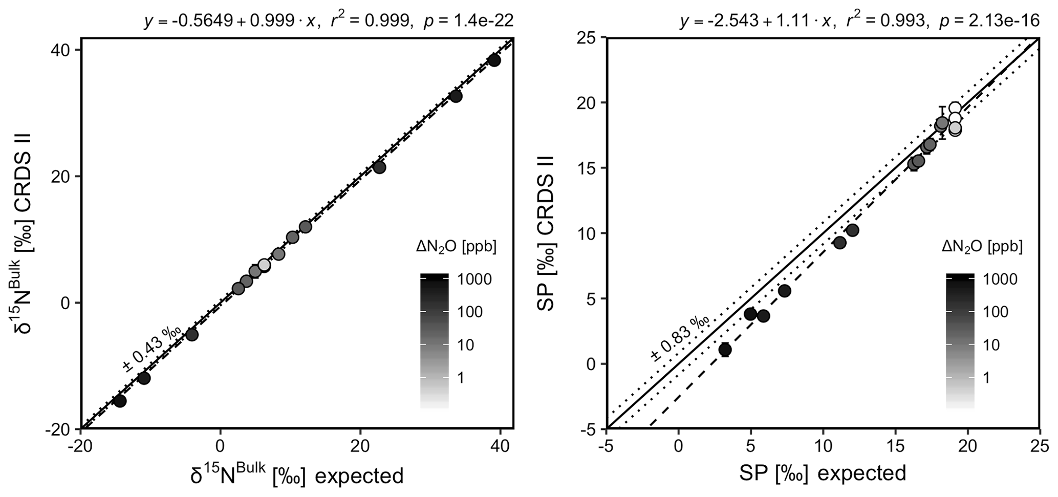
Figure 11Correlation diagrams for δ15Nbulk and SP measurements at various ΔN2O mole fractions analyzed by CRDS II plotted against expected values. The remaining plots for [N2O], δ15Nα, δ15Nβ and δ18O are provided in Sect. S4 (Fig. S4-12). The solid black line denotes the 1:1 line, while the dotted line indicates ±1σ of the residuals from the 1:1 line. The dashed black line represents a linear fit to the data. Individual equations, coefficients of determination (r2) and p values are indicated above each plot. Each data point represents the mean and standard deviation (1σ) of triplicate measurements. The inset plots indicate the standard deviation (1σ) of the triplicate measurements achieved at different ΔN2O mole fractions, and the 1:1 line is similarly a solid line.
QCLAS I
There was good agreement of [N2O] between QCLAS I and expected values; however, the analyzer underestimated mole fractions at higher ΔN2O during Exps. 5 and 6. Unfortunately, it is clear from the large spread of isotope values depicted in Fig. 12 that the standardized calibration scheme selected for the two-end-member mixing tests was insufficient for acquiring accurate and precise isotopic measurements using QCLAS I. For this reason, we urge researchers not to overinterpret such results, as the implementation of a QCLAS-specific calibration procedure (in line with results from Sect. 3.1 and 3.3) would improve results dramatically. Nonetheless, QCLAS I obtained accurate results at higher N2O mole fractions (indicated in red in Figs. 12 and S4-13), such that when ΔN2O<700 ppb measurements were excluded, δ15Nα, δ15Nβ, δ15Nbulk and SP were within ±3.0 ‰, 1.4 ‰, 1.4 ‰ and 3.8 ‰ of calculated expected values, respectively. Similarly, QCLAS I showed good agreement with IRMS only at higher ΔN2O (>700 ppb; Fig. S9-5). Similar to OA-ICOS I, the standard deviations of QCLAS I triplicate isotope measurements decreased dramatically with increasing ΔN2O, improving from ∼10 ‰ during Exps. 1 and 2 to typically between 0.1 ‰ and 1 ‰ during Exps. 5 and 6. Conversely, the standard deviations of triplicate sample measurements for [N2O] increased with increasing ΔN2O, rising from <0.1 ppb during Exps. 1–4, to >1 ppb during Exps. 5 and 6. All QCLAS I [N2O] measurements had better 1σ repeatability than those acquired using GC. QCLAS I had triplicate isotope measurement standard deviations comparable to IRMS only at higher ΔN2O (>700 ppb).
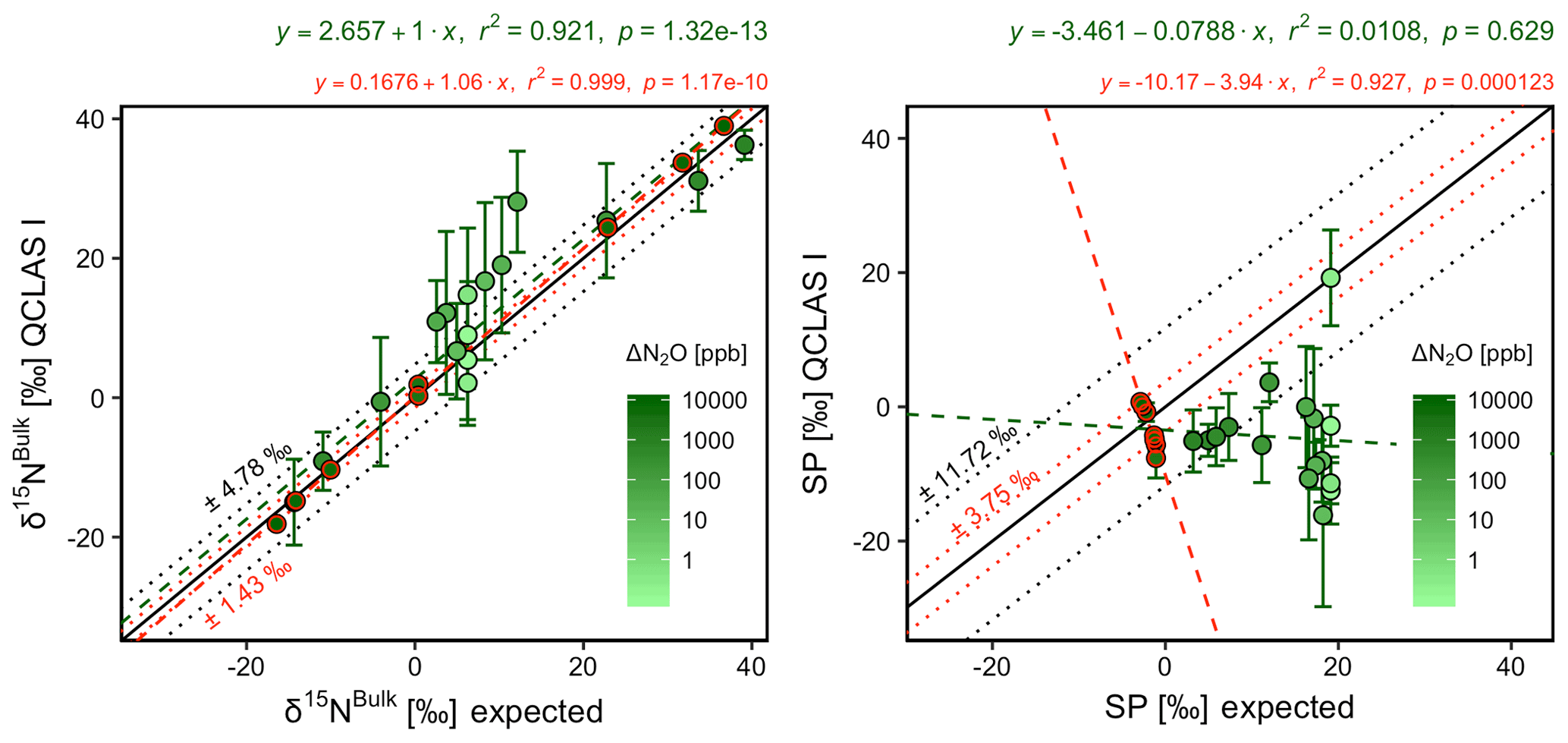
Figure 12Correlation diagrams for δ15Nbulk and SP measurements at various ΔN2O mole fractions analyzed by QCLAS I plotted against expected values. The remaining plots for [N2O], δ15Nα, δ15Nβ and δ18O are provided in Sect. S4 (Fig. S4-13). The solid black line denotes the 1:1 line, while the dotted line indicates ±1σ of the residuals from the 1:1 line. The dashed green line represents a linear fit to the data. Individual equations, coefficients of determination (r2) and p values are indicated above each plot. Each data point represents the mean and standard deviation (1σ) of triplicate measurements. The inset plots indicate the standard deviation (1σ) of the triplicate measurements achieved at different ΔN2O mole fractions, and the 1:1 line is similarly a solid line. Results for Exps. 5–6 are highlighted in red, with the dashed red line indicating a linear fit to this data.
TREX-QCLAS I
There was good agreement of N2O mixing ratios between the TREX-QCLAS I and expected values. Similarly, there was excellent agreement between the TREX-QCLAS I and calculated expected isotope values (all r2>0.97; Figs. 13 and S4-14). Measurements for δ15Nα, δ15Nβ, δ15Nbulk and SP were within ±0.29 ‰, 0.32 ‰, 0.23 ‰ and 0.41 ‰ of expected values, respectively. δ18O measurements were typically within ±0.24 ‰ of expected values. Generally, the standard deviations of triplicate isotope measurements decreased with increasing ΔN2O, improving from typically 0.2 ‰–0.3 ‰ at low ΔN2O mole fractions (ambient) to close to or better than 0.1 ‰ when ΔN2O reached 30 ppb. Conversely, the standard deviations of triplicate sample measurements for [N2O] increased with increasing ΔN2O, rising from <0.3 to ∼1 ppb. No comparison could be made between TREX-QCLAS I and IRMS measurements because TREX-QCLAS measurements were undertaken separately from the other instruments.
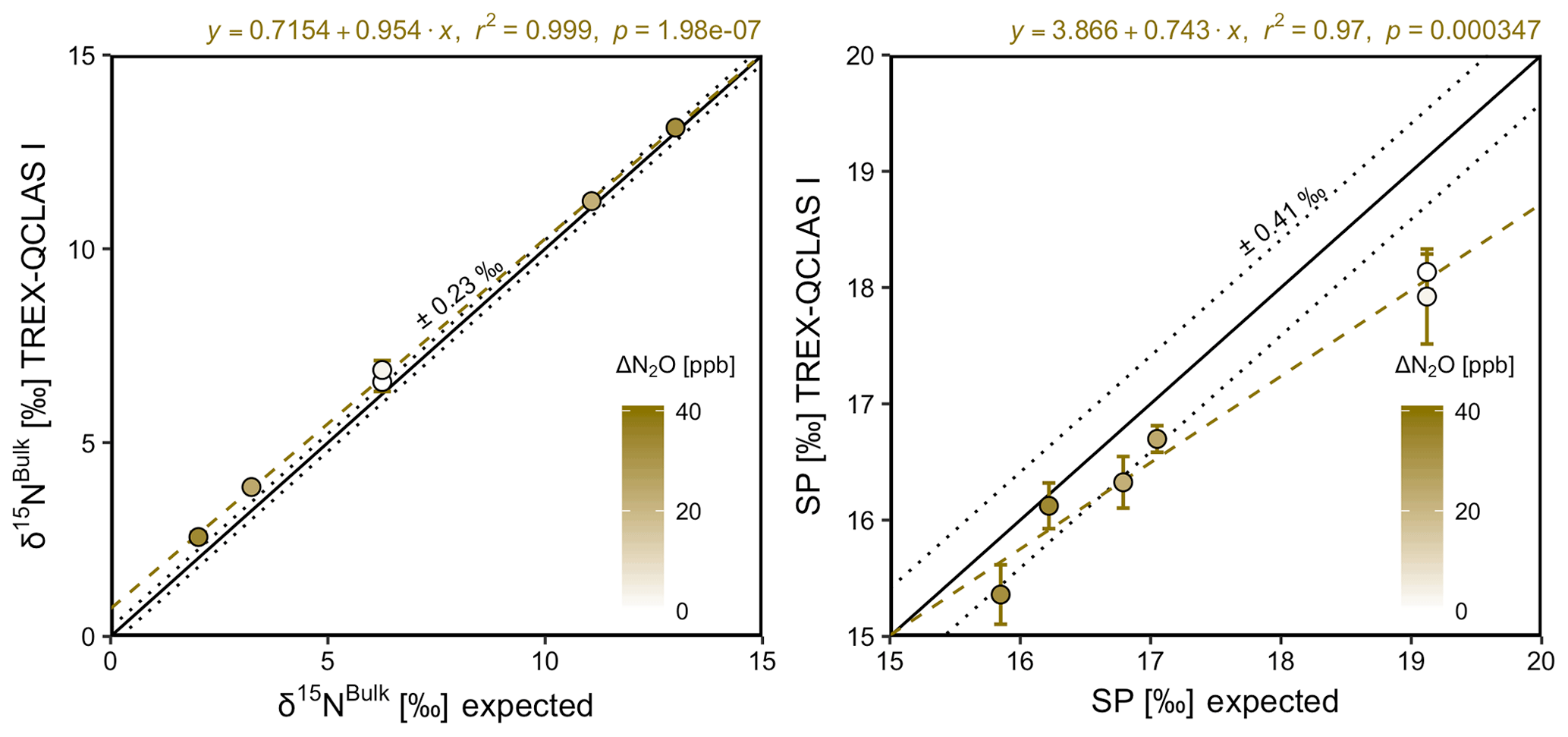
Figure 13Correlation diagrams for δ15Nbulk and SP measurements at various ΔN2O mole fractions analyzed by OA-ICOS I plotted against expected values. The remaining plots for [N2O], δ15Nα, δ15Nβ and δ18O are provided in Sect. S4 (Fig. S4-14). The solid black line denotes the 1:1 line, while the dotted line indicates ±1σ of the residuals from the 1:1 line. The dashed green line represents a linear fit to the data. Individual equations, coefficients of determination (r2) and p values are indicated above each plot. Each data point represents the mean and standard deviation (1σ) of triplicate measurements. The inset plots indicate the standard deviation (1σ) of the triplicate measurements achieved at different ΔN2O mole fractions, and the 1:1 line is similarly a solid line.
3.7.2 Source identification using Keeling analysis
Despite the excellent agreement between expected and measured values across all experiments for OA-ICOS I, CRDS I and II, and TREX-QCLAS I, the extrapolated source intercept values acquired using Keeling analysis showed large standard errors, especially for Exps. 1 and 2 (ΔN2O=30 ppb) (Figs. 14 and S4-15; Sect. S10). This was mostly due to the small mole fraction range (i.e., large inverse mole fraction range) over which the regression line was extrapolated in order to acquire the intercept value. The cause of the erroneous intercepts values was likely two-fold: (1) the extrapolated source was highly susceptible to measurements acquired at background levels, and due to the inherent greater uncertainty associated with measurements acquired at ambient N2O mole fractions, intercepts can be skewed accordingly; and (2) any further non-linearity that could not be taken into account in the three-point concentration dependence correction applied. Overall, this implies that N2O isotope source studies using laser spectroscopy focusing on near-ambient N2O variations remain a challenging undertaking, and one should expect large uncertainty in source estimates over small mole fraction changes.
For Exps. 3–6, however, the accuracy of the source intercept and its standard error improved dramatically for all analyzers on account of the decreasing uncertainty in measurement. OA-ICOS I and both CRDS analyzers typically achieved within ±2 ‰–5 ‰ of the assigned values for δ15Nα, δ15Nβ, δ15Nbulk, SP and δ18O, and had performance comparable to or better than the GC-IRMS approach (Figs. 14 and S4-15). Similarly, the standard error of all intercepts decreased dramatically for Exps. 3–6, and all analyzers typically achieved better than ±1 ‰ standard error on derived intercepts in Exps. 5 and 6.
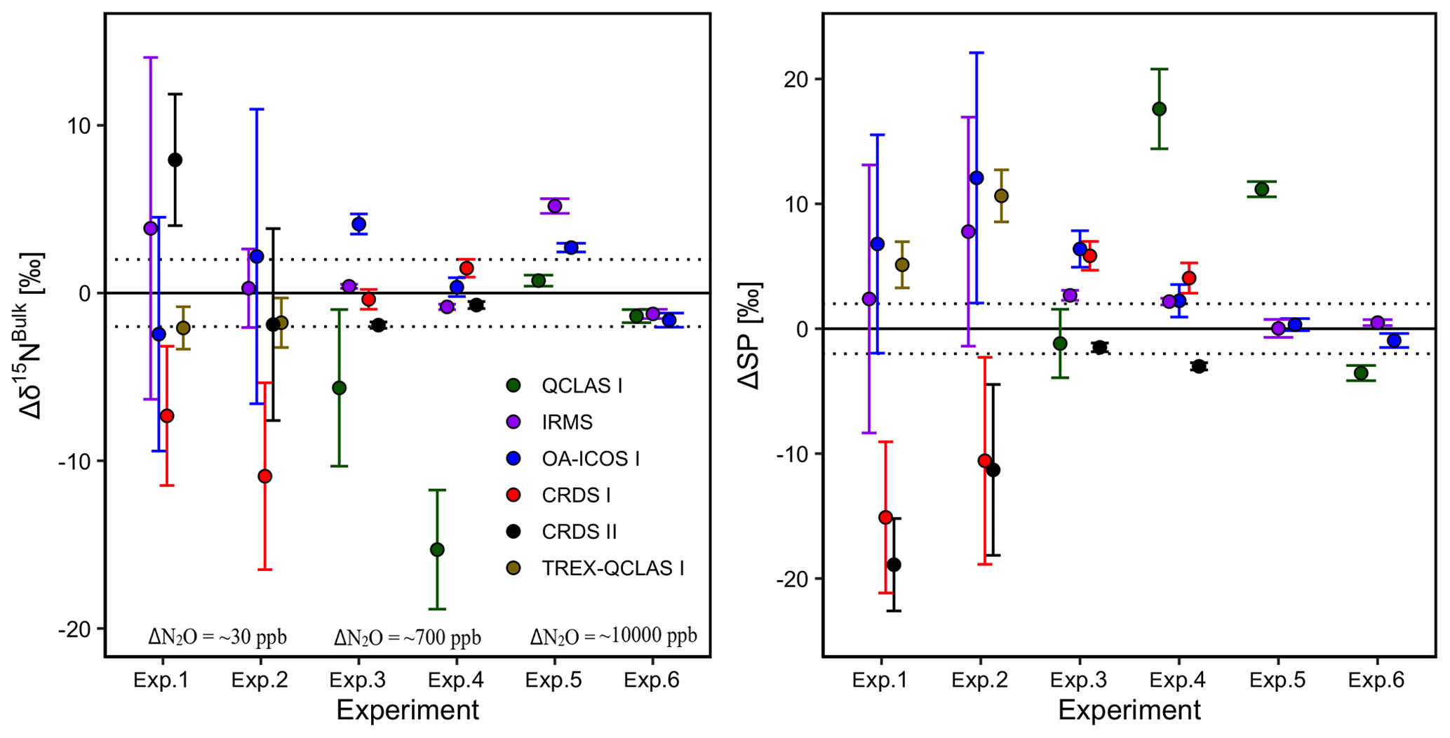
Figure 14Δδ15Nbulk and ΔSP(EstimatedSource−TrueSource) values derived from the OA-ICOS I (blue), CRDS I (red), CRDS II (black), QCLAS I (green) and IRMS (purple) via Keeling analysis of the two-end-member mixing scenario. The remaining plots for δ15Nα, δ15Nβ and δ18O are provided in Sect. S4 (Fig. S4-15). EstimatedSource=TrueSource is indicated by a solid black line at y=0, and the dotted lines indicated ±2 ‰ deviation from y=0. The change in concentration exceeding that of the background gas is indicated for Exps. 1–2 ( ppb), 3–4 ( ppb) and 5–6 ( ppb). Note that the QCLAS I results for Exps. 1 and 2 are not depicted to maintain clarity, as they exceed the selected y-axis scale.
4.1 Factors affecting the precision and accuracy of N2O isotopocule measurements using laser spectroscopy
A summary of results is presented in Table 8. Our results highlight that the precision at which laser-based analyzers acquire N2O isotopocule measurements is a function of N2O mole fraction, the selected measuring and averaging times and calibration frequency according to measurement stability. The degree of accuracy obtained using different laser spectrometers is ultimately a function of the robustness of corrections aimed at removing matrix and trace gas effects, and the selected calibration procedure aimed at standardizing the data to international scales.
Table 8Summary of main findings presented in this study.
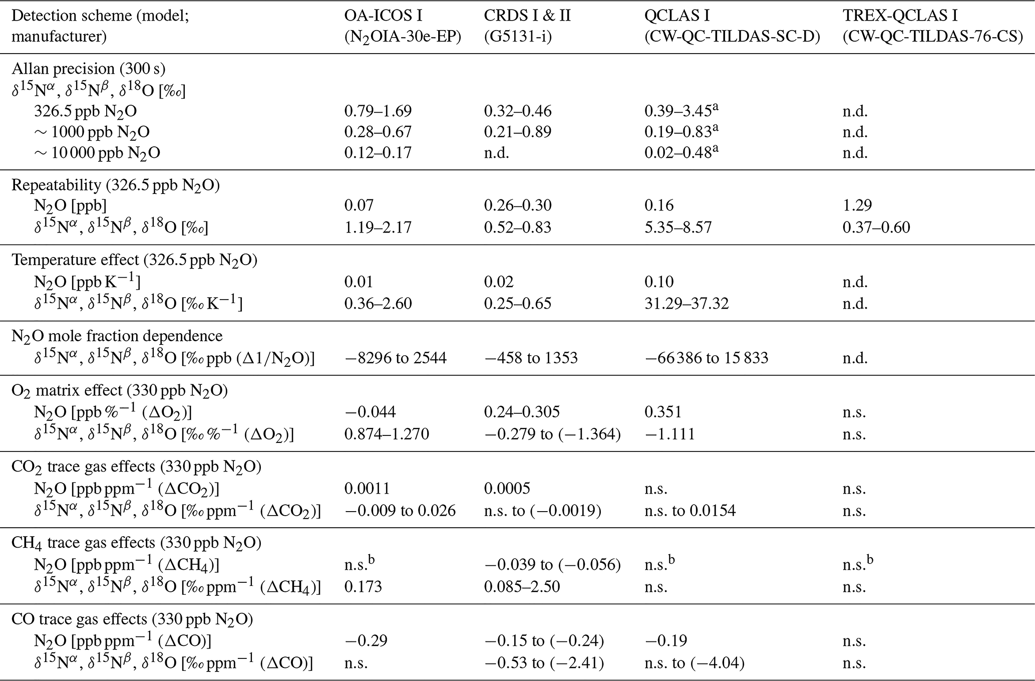
a Includes QCLAS I, II and III. b Likely due to inaccuracies during dynamic dilution (see text for details). n.d.: not determined. n.s.: not statistically significant at p<0.05 and/or r2<0.5.
All spectrometers tested displayed temperature effects on isotope measurements, which can be attributed to differences in the lower state energies of the probed N2O isotopocule lines (Sect. S11) (e.g., Wächter et al., 2008). The temperature sensitivities of all analyzers tested necessitates that, especially when deployed in the field, they be operated under temperature-controlled conditions (such as in maintained field stations).
The experiments performed in this study were undertaken using a standardized protocol. Calibration was performed on isotope δ values derived from raw uncalibrated isotopocule amount fractions, thus requiring [N2O] dependence corrections. Alternative approaches aimed at calibrating isotopocule amount fractions prior to deriving δ values were not included in our study but have the potential to remove the need for this correction (e.g., Wen et al., 2013; Flores et al., 2017; Griffith, 2018) if appropriate reference materials become available. Isotopocule calibration approaches would require a set of N2O standard gases with high-accuracy mole fractions in addition to assigned δ values.
All analyzers tested in this study showed significant effects from changing O2 composition of the gas matrix. Although the magnitude of this effect ultimately varied across the analyzers and was dependent on N2O mixing ratios, the effect of a change in O2 composition of 20.5 % was typically on the order of 10 ‰ to 30 ‰ for δ values. Similar O2 dependencies have been reported by Erler et al. (2015) for CRDS N2O isotope laser spectrometers, as well as for CRDS H2O isotope analyzers (Johnson and Rella, 2017). The underlying reason for this effect is differences in N2 versus O2 (and Ar) broadening parameters of the probed N2O isotopocule lines. In short, the N2, O2 (and Ar) broadening parameters depend on rotational quantum numbers of the respective N2O lines (Henry et al., 1985; Sect. S11). Thus, differences in the rotational quantum numbers for a pair of isotopocules (e.g., 14N15N16O∕14N14N16O) relate to a difference in their N2, O2 and Ar broadening parameters. Consequently, differences in the O2 or Ar content of the sample gas matrix and that of the reference gas affect measured isotope ratios and lead to changes in apparent δ values. Nonetheless, the magnitude of effects reported for the CRDS analyzers in this study varied across CRDS I (a 2015 model) and CRDS II (a 2018 model), as well as from those reported by Erler et al. (2015). Therefore, we recommended that in applications where O2 concentrations vary, such as groundwater, estuaries, stratified waterbodies and incubation studies, researchers test individual analyzers for their specific dependencies to allow for correction. This is especially important given that N2O production and reduction processes in such environments are strongly controlled by O2 availability. Although the Ar effects characterized in this study were not large, it is nonetheless recommended as a precautionary measure that researchers ensure, where possible, the standard calibration gas Ar composition is similar to that of the sample gas.
The CO2 effects for OA-ICOS and CH4 effects for CRDS analyzers must be considered for applications of these analyzers where CO2 and CH4 may also co-vary, such as during diel atmospheric monitoring, in soil-flux chamber measurements, incubation studies and even waterbodies (e.g., Erler et al., 2015). These effects need to be either characterized and corrected for by the user, or the interfering gas quantitatively removed. To our knowledge, there is currently no commercially available technique to remove CH4 from a gas stream without affecting N2O, and therefore independent co-analysis of CH4 is ultimately required to correct for these effects post-measurement. Similarly, while water vapor effects can in theory be characterized and corrected for all instruments, we recommend that researchers remove water vapor from the gas stream prior to analysis. Although not tested here, other studies have highlighted possible spectral interference effects associated with elevated H2S and volatile organic compounds (Erler et al., 2015; Ostrom and Ostrom, 2017), but these may also be removed from gas streams using chemical traps (e.g., Cu and activated carbon traps, respectively).
The scaling of gas matrix and trace gas effects with [N2O] has important implications for any measurement setup that relies on post-measurement correction equations. An equation developed to correct for CH4 effects that was derived using a [N2O] of 330 ppb should not be implemented for a sample gas containing 990 ppb N2O. For example, as shown in Fig. 8, the measured interference effect on δ15Nα measurements acquired using CRDS II for 10 ppm [CH4] at 330 ppb N2O was 24.9 ‰, while at 990 ppb N2O it was 8.1 ‰, resulting in a 16.8 ‰ difference. The scaling of interference effects from trace gases has been reported previously for CO2∕CH4 laser spectrometers (Assan et al., 2017; Malowany et al., 2015). This underlines the usefulness of removing H2O, CO2 and CO with scrubbers prior to measurement, as this removes the need for correction equations to begin with and the scaling of corrections that can ensue. We are unaware of any studies that have shown that O2 interferences caused by pressure-broadening linewidth effects change as a function of N2O mole fraction. While we were unable to describe the scaling of the O2 effect sufficiently using correction functions based on theoretical deductions, empirical equations based on experimental testing, such as those developed in Sect. 3.5.2 and 3.6.2, could be implemented by researchers when covariation in both O2 and N2O in the sample gas is expected. Alternatively, as shown in this study, matrix and/or trace gas effects can be removed by automated N2O preconcentration devices such as TREX (Ibraim et al., 2018; Mohn et al., 2010), similar to IRMS. However, such devices are not commercially available, complex to build and operate, and restrict sample frequency.
4.2 Pre-measurement considerations
Our study clearly shows that knowledge/estimation of the matrix and trace gas composition of both reference standards and sample gases, and the differences between them, are critical for accurate N2O isotopocule analysis using laser spectroscopy. We acknowledge, however, that this may be difficult to predict in certain applications without prior testing of the sample gas, and therefore researchers should err on the side of caution.
As a prerequisite to acquiring measurements using N2O isotope laser spectrometers, researchers will be required to consider the accessory gas mixtures required to characterize their instrument. For applications with significant variations in matrix (O2, Ar) or trace gas (CO2, CH4, CO) compositions, researchers will require gas mixtures containing the gas of interest in order to characterize the associated interference effects for their laser spectrometer. This also necessitates that appropriate interference detectors are implemented, especially O2 and CH4 analyzers given that these effects cannot be mitigated using chemical traps.
In this study, interference effects, and the associated scaling of these effects according to the co-measured N2O mole fraction, were derived via dynamic dilution with various gas mixtures using MFCs. This allowed for the introduction of a wide range of gas mixtures to the analyzers for interference testing, and consequently only a small amount of gas mixtures were required for all of the experiments outlined in Sect. 2.4. In comparison, a much larger number of individual gas mixtures would have been required had they been prepared using static dilution techniques (see Erler et al., 2015). The scaling of interference effects was sufficiently distinguished by undertaking testing at three different N2O mole fractions (N2O=330, 660 and 990 ppb), and we therefore recommend this as a minimum criterion for researchers wishing to characterize this effect.
Researchers should also consider the sample gas volume required for a given measurement application using a specific laser spectrometer. In our experience, ensuring that five laser cavity cell volumes have been flushed prior to measurement is best practice to negate any memory effects when these instruments are operated using continuous flow-through configurations (as opposed to discrete sample measurements in a closed laser cavity). By following this procedure and using the operating parameters selected in this study (Table 1), the sample gas volume required for a single 300 s measurement is approximately 80 mL for CRDS II, 150 mL for CRDS I, 600 mL for OA-ICOS I and 1200 mL for QCLAS I. By comparison, TREX-QCLAS I requires approximately 5 L of sample gas to allow for N2O preconcentration. These sample gas volumes represent typical numbers for atmospheric applications; however, instrument parameter settings such as flow rate and cell pressure, which ultimately change the required sample volume, can be optimized depending on the measurement application. This is particularly the case for QCLAS instruments, which can be operated with different user-adjustable settings. For applications requiring discrete sample analysis (e.g., the headspace analysis of δ15N and δ18O in N2O derived from dissolved ), high N2O concentration gas samples with lower volumes can be introduced to these instruments using injection ports and dilution gases (e.g., Soto et al., 2015; Wassenaar et al., 2018); however, we did not test these capabilities in our study.
4.3 Measurement workflow
In line with our results, we propose a step-by-step workflow that can be followed by researchers to acquire N2O isotopocule measurements (Fig. 15). This workflow seeks to cover all sources of potential error tested in our study. Not all steps will be applicable because interference effects vary across analyzers. For QCLAS analyzers, which offer high versatility, interference effects can also be approached by multi-line analysis, inclusion of interfering spectral lines or adaption of pressure-broadening parameters in the spectral fitting algorithm. For specific applications, such as incubation experiments with He, accessory injection units and setups using TREX, related actions have to be taken. While we tested several mono-variant (e.g., changes in [CH4] at constant [N2O]) and some bi-variant (e.g., changes in [CH4] and [N2O]) systems in our study, more complex systems (e.g., changes in [CH4], [O2] and [N2O]) were not tested, and deviations from additive behavior are to be expected. Depending on the desired precision, users may vary the measurement and averaging times, and calibration frequency.
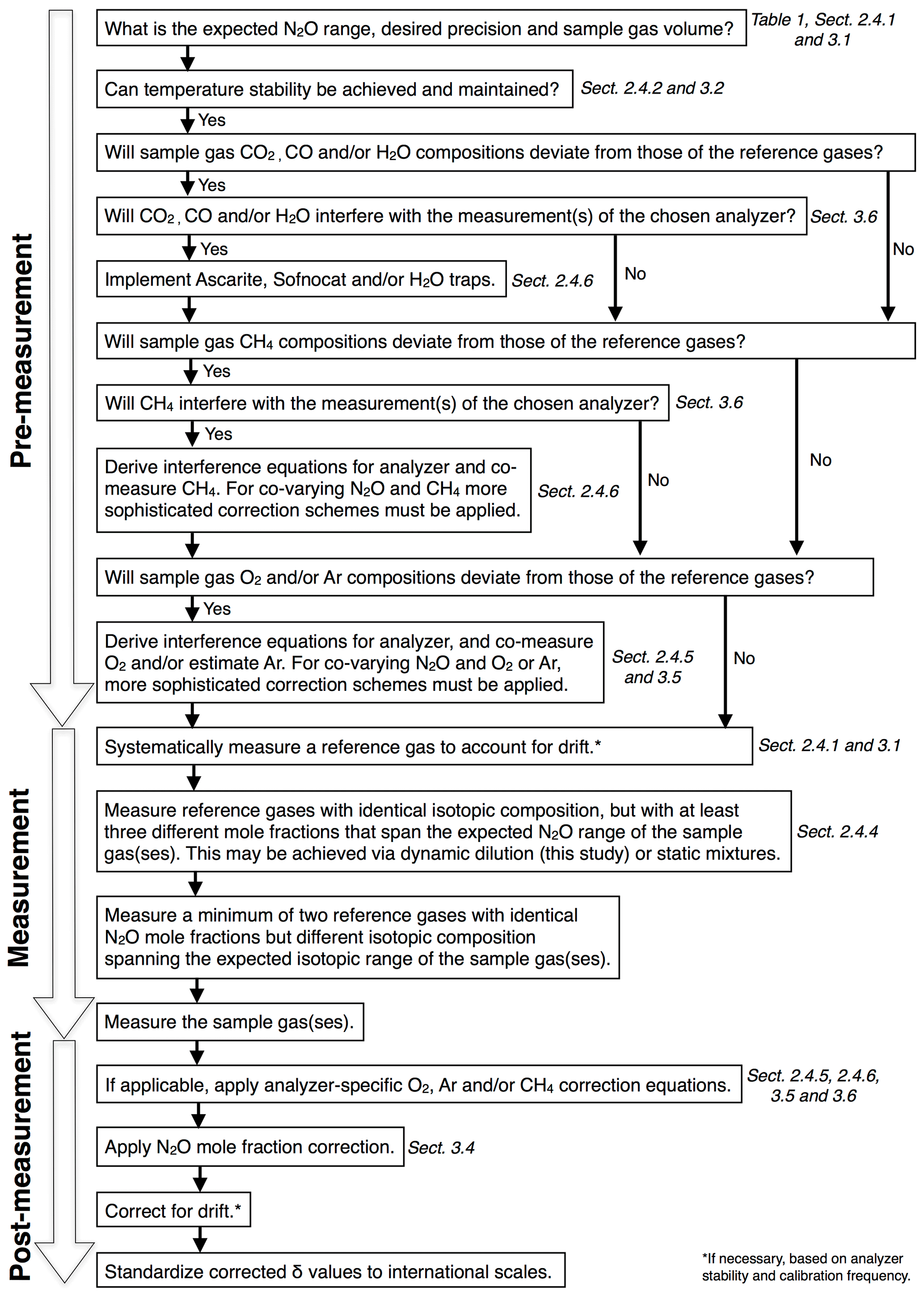
Figure 15Proposed measurement workflow for the operation of N2O isotope laser spectrometers. Relevant sections of this study are shown next to each step.
4.4 What degree of accuracy can be achieved using this workflow?
The simulated two-end-member mixing experiments conducted in this study show that, when the workflow proposed above is applied, accuracy within ±0.5 ‰ can be achieved for TREX-QCLAS, ±0.4 ‰–1.6 ‰ for CRDS analyzers and ±1.6 ‰–3.6 ‰ for OA-ICOS analyzers. Likewise, the comparison between the laser spectrometers and IRMS highlights that cross-technique compatibility within ±1 ‰–2.5 ‰ can be achieved for most N2O isotopocule measurements. However, it is clear that the balanced (i.e., non-analyzer-specific) approach applied for the purpose of this comparative study did not cater to QCLAS I. Therefore, a more specific calibration protocol for the QCLAS I will likely yield better performance, as shown in Table 6. It is worth noting that, although the results of our study are representative of the performance of the instruments tested, the magnitude of reported effects and the performance are likely to vary within the same analyzer models.
Whilst the laboratory-simulated mixing experiment is not fully representative of naturally occurring two-end-member mixing per se, the results are useful in comparing intercept accuracy and uncertainty amongst analyzers and against IRMS. Our results show that large uncertainties exist for N2O source apportionment using Keeling analysis performed at near-ambient N2O mole fractions. Given the amount of corrections that are required in the experiment, we have not detailed individual analyzer uncertainty budgets to quantify individual sources of error on the intercept, as it is beyond the scope of this study. Nonetheless, the reduction of uncertainty with increasing ΔN2O shown in Exps. 1–6 in Sect. 3.7 has also been shown in previous studies (e.g., Wolf et al., 2015). Therefore, by extension, it is reasonable to assume that the current largest source of uncertainty for ambient N2O measurements using laser spectroscopy is the inherent signal-to-noise ratio of the measurement.
In this study, we characterized and compared N2O isotope laser-based analyzers with the three most common detection schemes, including OA-ICOS, CRDS and QCLAS. Our results show a number of factors that need to be carefully considered to ensure precise and accurate measurements of N2O isotopocules using laser spectroscopy. The performance of N2O isotope laser spectrometers depends on a complex interplay between instrumental precision, drift, matrix gas composition and associated spectral interferences that ultimately vary as a function of N2O mole fraction. On this basis, we echo recommendations from Ostrom and Ostrom (2017), who cautioned not to underestimate the need for the careful consideration of analyzer-specific corrections. These analyzers clearly do not represent “plug and play” devices – instead, one needs to carefully consider the desired application, precision and accuracy, and develop appropriate calibration strategies to achieve these outcomes.
Consequently, we recommend calibration schemes that have (1) a calibration frequency that is adequate for constraining instrument drift over experimental period/long-term measurements; (2) temperature stability during measurement, or the temperature effect adequately characterized and corrected; (3) a three-point or higher [N2O] effect correction that spans the range of expected [N2O] (if calibration relies on raw δ values derived from uncalibrated isotopocule amount fractions; i.e., a δ-calibration approach); and (4) accounted for the differences in matrix and trace gas composition between the sample gas and reference gases, whereby either analyzer-specific interference corrections have been carefully characterized and applied, or where possible interfering substances (CO2, CO, H2O) removed using chemical traps. Correcting for interference effects becomes significantly more complicated once [N2O] exceeds ambient levels, requiring a multitude of analyzer- and gas-specific constants that inevitably increase the number of gas mixtures required by the user, as well as the uncertainty of the measurement. Researchers should therefore strive to implement measurement setups that require as few corrections as possible, and this will inherently decrease the combined uncertainty in the measurement.
All data are available from the corresponding author upon request.
The supplement related to this article is available online at: https://doi.org/10.5194/amt-13-2797-2020-supplement.
SJH and JL, guided by JM, designed the study, established the setup and coordinated the experiments. Responsibilities of the analyzers were as follows: SJH, BFJK and DIC were responsible for OA-ICOS; JL and TB were responsible for CRDS I; LX and BW were responsible for QCLAS I and CRDS II; JW and KZ were responsible for TREX-QCLAS I; MB and JS were responsible for QCLAS II, QCLAS III and GC-IRMS. JM prepared the non-commercial gas mixtures used in this study. LY referenced the δ values of applied gas mixtures to international scales. SJH and JL performed the main data analysis and together with JM developed correction algorithms. SJH and JL wrote the manuscript with input from all co-authors.
The authors declare that they have no conflict of interest.
We extend our thanks to Doug Baer, Rob Provencal and Frederick Despagne from ABB – Los Gatos Research Inc., Renato Winkler, Magdalena Hofmann and Paulos Getachew from Picarro Inc., and Dave Nelson and Barry McManus from Aerodyne Research Inc. for their helpful discussions and assistance concerning the analyzers. We thank Christoph Zellweger for his assistance in analyzing matrix gas cylinders and providing the Picarro G2401 for matrix interference testing, and the NABEL laboratory at Empa for providing the dew-point generator for water vapor testing. We want to thank Kristýna Kantnerová from Empa and Daniel Zindel from ETH for the synthesis of 18O-labeled N2O.
This research has been supported by the Swiss National Science Foundation (grant nos. CRSII5_170876, 200021_163075), the Australian Endeavour Leadership Program (grant no. ERF_RDDH_6743_2018), the European Metrology Programme for Innovation and Research (EMPIR) co-funded by the European Union's Horizon 2020 research and innovation program and the EMPIR participating states (grant no. 16ENV06; Metrology for Stable Isotope Reference Standards (SIRS)), the Cotton Research and Development Corporation (CRDC) (grant no. ANSTO1801) and the H2020 Marie Skłodowska-Curie Actions (EMPAPOSTDOCS-II (grant no. 754364)).
Stephen Harris is supported by PhD scholarships from the Australian Government, the Australian Institute of Nuclear Science and Engineering (AINSE (scholarship no. RG172557)), Australian Nuclear Science and Technology Organisation (ANSTO) (scholarship no. RG171945) and CRDC (scholarship no. RG1626691). The UNSW Sydney N2OIA-30e-EP was purchased using funds from the Australian National Collaborative Research Infrastructure Strategy (NCRIS) Groundwater Infrastructure Project (grant no. RG134076). Jing Wei and Longfei Yu were supported by the Swiss National Science Foundation (SNSF) within grants CRSII5_170876 and 200021_163075, as well as the EMPAPOSTDOCS-II program, which received funding from the European Union's H2020 Marie Skłodowska-Curie Actions (EMPAPOSTDOCS-II (grant no. 754364)).
This paper was edited by Huilin Chen and reviewed by three anonymous referees.
ABB-Los Gatos Research Inc.: Off-Axis Integrated Cavity Output Spectroscopy (OA-ICOS), available at: http://www.lgrinc.com/advantages/, last access: 15 August 2019.
Allan, D. W.: Statistics of atomic frequency standards, P. IEEE, 54, 221–230, 1966.
Assan, S., Baudic, A., Guemri, A., Ciais, P., Gros, V., and Vogel, F. R.: Characterization of interferences to in situ observations of δ13CH4 and C2H6 when using a cavity ring-down spectrometer at industrial sites, Atmos. Meas. Tech., 10, 2077–2091, https://doi.org/10.5194/amt-10-2077-2017, 2017.
Baer, D. S., Paul, J. B., Gupta, M., and O'Keefe, A.: Sensitive absorption measurements in the near-infrared region using off-axis integrated-cavity-output spectroscopy, Appl. Phys. B-Lasers O., 75, 261–265, https://doi.org/10.1007/s00340-002-0971-z, 2002.
Baggs, E. M.: A review of stable isotope techniques for N2O source partitioning in soils: recent progress, remaining challenges and future considerations, Rapid Commun. Mass Sp., 22, 1664–1672, https://doi.org/10.1002/rcm.3456, 2008.
Berden, G., Peeters, R., and Meijer, G.: Cavity ring-down spectroscopy: Experimental schemes and applications, Int. Rev. Phys. Chem., 19, 565–607, https://doi.org/10.1080/014423500750040627, 2000.
Bernard, S., Röckmann, T., Kaiser, J., Barnola, J.-M., Fischer, H., Blunier, T., and Chappellaz, J.: Constraints on N2O budget changes since pre-industrial time from new firn air and ice core isotope measurements, Atmos. Chem. Phys., 6, 493–503, https://doi.org/10.5194/acp-6-493-2006, 2006.
Bouwman, A. F., Boumans, L. J. M., and Batjes, N. H.: Modeling global annual N2O and NO emissions from fertilized fields, Global Biogeochem. Cy., 16, 1080, https://doi.org/10.1029/2001GB001812, 2002.
Bowling, D. R., Sargent, S. D., Tanner, B. D., and Ehleringer, J. R.: Tunable diode laser absorption spectroscopy for stable isotope studies of ecosystem-atmosphere CO2 exchange, Agr. Forest Meteorol., 118, 1–19, https://doi.org/10.1016/s0168-1923(03)00074-1, 2003.
Bowling, D. R., Burns, S. P., Conway, T. J., Monson, R. K., and White, J. W. C.: Extensive observations of CO2 carbon isotope content in and above a high-elevation subalpine forest, Global Biogeochem. Cy., 19, GB3023, https://doi.org/10.1029/2004gb002394, 2005.
Brase, L., Bange, H. W., Lendt, R., Sanders, T., and Dähnke, K.: High Resolution Measurements of Nitrous Oxide (N2O) in the Elbe Estuary, Front. Mar. Sci., 4, 162, https://doi.org/10.3389/fmars.2017.00162, 2017.
Buchen, C., Lewicka-Szczebak, D., Flessa, H., and Well, R.: Estimating N2O processes during grassland renewal and grassland conversion to maize cropping using N2O isotopocules, Rapid Commun. Mass Sp., 32, 1053–1067, https://doi.org/10.1002/rcm.8132, 2018.
Decock, C. and Six, J.: How reliable is the intramolecular distribution of 15N in N2O to source partition N2O emitted from soil?, Soil Biol. Biochem., 65, 114–127, https://doi.org/10.1016/j.soilbio.2013.05.012, 2013.
Denk, T. R., Mohn, J., Decock, C., Lewicka-Szczebak, D., Harris, E., Butterbach-Bahl, K., Kiese, R., and Wolf, B.: The nitrogen cycle: A review of isotope effects and isotope modeling approaches, Soil Biol Biochem., 105, 121–137, https://doi.org/10.1016/j.soilbio.2016.11.015, 2017.
Denman, K. L., Brasseur, G., Chidthaisong, A., Ciais, P., Cox, P. M., Dickinson, R. E., Hauglustaine, D., Heinze, C., Holland, E., Jacob, D., Lohmann, U., Ramachandran, S., da Silva Dias, P. L., Wofsky, S. C., and Zhang, X.: Couplings between changes in the climate system and biogeochemistry, in: Climate change 2007, the physical science basis, contribution of working group I to the Fourth Assessment Report of the Intergovernmental Panel on Climate Change, edited by: Solomon, S., Qin, D., Manning, M., Chen, Z., Marquis, M., Averyt, K. B., Tignor, M., and Miller, H. L., Cambridge University Press, Cambridge, United Kingdom and New York, NY, USA, 499–587, 2007.
Erler, D. V., Duncan, T. M., Murray, R., Maher, D. T., Santos, I. R., Gatland, J. R., Mangion, P., and Eyre, B. D.: Applying cavity ring-down spectroscopy for the measurement of dissolved nitrous oxide mole fractions and bulk nitrogen isotopic composition in aquatic systems: Correcting for interferences and field application, Limnol. Oceanogr.-Meth., 13, 391–401, https://doi.org/10.1002/lom3.10032, 2015.
Eyer, S., Tuzson, B., Popa, M. E., van der Veen, C., Röckmann, T., Rothe, M., Brand, W. A., Fisher, R., Lowry, D., Nisbet, E. G., Brennwald, M. S., Harris, E., Zellweger, C., Emmenegger, L., Fischer, H., and Mohn, J.: Real-time analysis of δ13C- and δD−CH4 in ambient air with laser spectroscopy: method development and first intercomparison results, Atmos. Meas. Tech., 9, 263–280, https://doi.org/10.5194/amt-9-263-2016, 2016.
Flores, E., Viallon, J., Moussay, P., Griffith, D. W., and Wielgosz, R. I.: Calibration strategies for FT-IR and other isotope ratio infrared spectrometer instruments for accurate δ13C and δ18O measurements of CO2 in air, Anal. Chem., 89, 3648–3655, https://doi.org/10.1021/acs.analchem.6b05063, 2017.
Forster, P., Ramaswamy, V., Artaxo, P., Berntsen, T., Betts, R., Fahey, D. W., Haywood, J., Lean, J., Lowe, D. C., Myhre, G., Nganga, J., Prinn, R., Raga, G., Schulz, M., and Van Dorland, R.: Climate Change 2007: Changes in Atmospheric Constituents and in Radiative Forcing, The Physical Science Basis: Contribution of Working Group I to the Fourth Assessment Report of the Intergovernmental Panel on Climate Change, edited by: Solomon, S., Qin, D., Manning, M., Chen, Z., Marquis, M., Averyt, K. B., Tignor, M., and Miller, H. S., Cambridge University Press, Cambridge, UK, New York, NY, USA, 2007.
Friedrichs, G., Bock, J., Temps, F., Fietzek, P., Körtzinger, A., and Wallace, D. W.: Toward continuous monitoring of seawater 13CO2∕12CO2 isotope ratio and pCO2: Performance of cavity ringdown spectroscopy and gas matrix effects, Limnol. Oceanogr.-Meth., 8, 539–551, https://doi.org/10.4319/lom.2010.8.539, 2010.
Griffis, T. J., Baker, J. M., Sargent, S. D., Tanner, B. D., and Zhang, J.: Measuring field-scale isotopic CO2 fluxes with tunable diode laser absorption spectroscopy and micrometeorological techniques, Agr. Forest Meteorol., 124, 15–29, https://doi.org/10.1016/j.agrformet.2004.01.009, 2004.
Griffith, D. W. T.: Calibration of isotopologue-specific optical trace gas analysers: a practical guide, Atmos. Meas. Tech., 11, 6189–6201, https://doi.org/10.5194/amt-11-6189-2018, 2018.
Griffith, D. W. T., Deutscher, N. M., Caldow, C., Kettlewell, G., Riggenbach, M., and Hammer, S.: A Fourier transform infrared trace gas and isotope analyser for atmospheric applications, Atmos. Meas. Tech., 5, 2481–2498, https://doi.org/10.5194/amt-5-2481-2012, 2012.
Gröning, M.: TEL Technical Note No. 01. SICalib User Manual (Stable Isotope Calibration for routine δ-scale measurements) Ver 2.16j, 2018.
Harris, E., Nelson, D. D., Olszewski, W., Zahniser, M., Potter, K. E., McManus, B. J., Whitehill, A., Prinn, R. G., and Ono, S.: Development of a spectroscopic technique for continuous online monitoring of oxygen and site-specific nitrogen isotopic composition of atmospheric nitrous oxide, Anal. Chem., 86, 1726–1734, https://doi.org/10.1021/ac403606u, 2014.
Harris, E., Joss, A., Emmenegger, L., Kipf, M., Wolf, B., Mohn, J. and Wunderlin, P.: Isotopic evidence for nitrous oxide production pathways in a partial nitritation-anammox reactor, Water Res., 83, 258–270, https://doi.org/10.1016/j.watres.2015.06.040, 2015a.
Harris, E., Zeyer, K., Kegel, R., Müller, B., Emmenegger, L., and Mohn, J.: Nitrous oxide and methane emissions and nitrous oxide isotopic composition from waste incineration in Switzerland, Waste Manage., 35, 135–140, https://doi.org/10.1016/j.wasman.2014.10.016, 2015b.
Harris, E., Henne, S., Hüglin, C., Zellweger, C., Tuzson, B., Ibraim, E., Emmenegger L., and Mohn J.: Tracking nitrous oxide emission processes at a suburban site with semicontinuous, in situ measurements of isotopic composition, J. Geophys. Res.-Atmos., 122, 1850–1870, https://doi.org/10.1002/2016JD025906, 2017.
Heil, J., Wolf, B., Brüggemann, N., Emmenegger, L., Tuzson, B., Vereecken, H., and Mohn, J.: Site-specific 15N isotopic signatures of abiotically produced N2O, Geochim. Cosmochim. Ac., 139, 72–82, https://doi.org/10.1016/j.gca.2014.04.037, 2014.
Henry, A., Margottin-Maclou, M., and Lacome, N.: N2- and O2-broadening parameters in the ν3 band of , J. Mol. Spectrosc., 111, 291–300, https://doi.org/10.1016/0022-2852(85)90006-2, 1985.
Ibraim, E., Harris, E., Eyer S., Tuzson, B., Emmenegger, L., Six, J., and Mohn, J.: Development of a field-deployable method for simultaneous, real-time measurements of the four most abundant N2O isotopocules, Isot. Environ. Health S., 54, 1–5, https://doi.org/10.1080/10256016.2017.1345902, 2018.
Ibraim, E., Wolf, B., Harris, E., Gasche, R., Wei, J., Yu, L., Kiese, R., Eggleston, S., Butterbach-Bahl, K., Zeeman, M., Tuzson, B., Emmenegger, L., Six, J., Henne, S., and Mohn, J.: Attribution of N2O sources in a grassland soil with laser spectroscopy based isotopocule analysis, Biogeosciences, 16, 3247–3266, https://doi.org/10.5194/bg-16-3247-2019, 2019.
Ishijima, K., Sugawara, S., Kawamura, K., Hashida, G., Morimoto, S., Murayama, S., Aoki, S., and Nakazawa, T.: Temporal variations of the atmospheric nitrous oxide mole fraction and its δ15N and δ18O for the latter half of the 20th century reconstructed from firn air analyses, J. Geophys. Res., 112, D03305, https://doi.org/10.1029/2006JD007208, 2007.
Ji, Q. and Grundle, D. S.: An automated, laser-based measurement system for nitrous oxide isotope and isotopomer ratios at nanomolar levels, Rapid Commun. Mass Sp., 33, 1553–1564, https://doi.org/10.1002/rcm.8502, 2019.
Johnson, J. E. and Rella, C. W.: Effects of variation in background mixing ratios of N2, O2, and Ar on the measurement of δ18O−H2O and δ2H−H2O values by cavity ring-down spectroscopy, Atmos. Meas. Tech., 10, 3073–3091, https://doi.org/10.5194/amt-10-3073-2017, 2017.
Keeling, C. D.: The mole fraction and isotopic abundances of atmospheric carbon dioxide in rural areas, Geochim. Cosmochim. Ac., 13, 322–334, https://doi.org/10.1016/0016-7037(58)90033-4, 1958.
Koba, K., Osaka, K., Tobari, Y., Toyoda, S., Ohte, N., Katsuyama, M., Suzuki, N., Itoh, M., Yamagishi, H., Kawasaki, M., and Kim, S. J.: Biogeochemistry of nitrous oxide in groundwater in a forested ecosystem elucidated by nitrous oxide isotopomer measurements, Geochim. Cosmochim. Ac., 73, 3115–3133, https://doi.org/10.1016/j.gca.2009.03.022, 2009.
Kong, X., Duan, Y., Schramm, A., Eriksen, J., Holmstrup, M., Larsen, T., Bol, R., and Petersen, S.O.: Mitigating N2O emissions from clover residues by 3,4-dimethylpyrazole phosphate (DMPP) without adverse effects on the earthworm Lumbricus terrestris, Soil Biol. Biochem., 104, 95–107, https://doi.org/10.1016/j.soilbio.2016.10.012, 2017.
Köster, J. R., Cárdenas, L., Senbayram, M., Bol, R., Well, R., Butler, M., Mühling, K. H., and Dittert, K.: Rapid shift from denitrification to nitrification in soil after biogas residue application as indicated by nitrous oxide isotopomers, Soil Biol. Biochem., 43, 1671–1677, https://doi.org/10.1016/j.soilbio.2011.04.004, 2011.
Köster, J. R., Well, R., Tuzson, B., Bol, R., Dittert, K., Giesemann, A., Emmenegger, L., Manninen, A., Cárdenas, L., and Mohn, J.: Novel laser spectroscopic technique for continuous analysis of N2O isotopomers – application and intercomparison with isotope ratio mass spectrometry, Rapid Commun. Mass Sp., 27, 216–222, https://doi.org/10.1002/rcm.6434, 2013.
Lebegue, B., Schmidt, M., Ramonet, M., Wastine, B., Yver Kwok, C., Laurent, O., Belviso, S., Guemri, A., Philippon, C., Smith, J., and Conil, S.: Comparison of nitrous oxide (N2O) analyzers for high-precision measurements of atmospheric mole fractions, Atmos. Meas. Tech., 9, 1221–1238, https://doi.org/10.5194/amt-9-1221-2016, 2016.
Lee, A., Winther, M., Priemé, A., Blunier, T., and Christensen, S.: Hot spots of N2O emission move with the seasonally mobile oxic-anoxic interface in drained organic soils, Soil Biol. Biochem., 115, 178–186, https://doi.org/10.1016/j.soilbio.2017.08.025, 2017.
Lewicka-Szczebak, D., Well, R., Köster, J. R., Fuß, R., Senbayram, M., Dittert, K., and Flessa, H.: Experimental determinations of isotopic fractionation factors associated with N2O production and reduction during denitrification in soils, Geochim. Cosmochim. Ac., 134, 55–73, https://doi.org/10.1016/j.gca.2014.03.010, 2014.
Lewicka-Szczebak, D., Well, R., Bol, R., Gregory, A. S., Matthews, G. P., Misselbrook, T., Whalley, W. R., and Cardenas, L. M.: Isotope fractionation factors controlling isotopocule signatures of soil-emitted N2O produced by denitrification processes of various rates, Rapid Commun. Mass Sp., 29, 269–282, https://doi.org/10.1002/rcm.7102, 2015.
Li, P., Wang, S., Peng, Y., Liu, Y., and He, J.: The synergistic effects of dissolved oxygen and pH on N2O production in biological domestic wastewater treatment under nitrifying conditions, Environ. Technol., 36, 1623–1631, https://doi.org/10.1080/09593330.2014.1002862, 2015.
Li, X., Sørensen, P., Olesen, J. E., and Petersen, S. O.: Evidence for denitrification as main source of N2O emission from residue-amended soil, Soil Biol. Biochem., 92, 153–160, https://doi.org/10.1016/j.soilbio.2015.10.008, 2016.
Malowany, K., Stix, J., Van Pelt, A., and Lucic, G.: H2S interference on CO2 isotopic measurements using a Picarro G1101-i cavity ring-down spectrometer, Atmos. Meas. Tech., 8, 4075–4082, https://doi.org/10.5194/amt-8-4075-2015, 2015.
Miller, J. B. and Tans, P. P.: Calculating isotopic fractionation from atmospheric measurements at various scales, Tellus B, 55, 207–214, https://doi.org/10.1034/j.1600-0889.2003.00020.x, 2003.
Minamikawa, K., Nishimura, S., Nakajima, Y., Osaka, K.I., Sawamoto, T., and Yagi, K.: Upward diffusion of nitrous oxide produced by denitrification near shallow groundwater table in the summer: a lysimeter experiment, Soil Sci. Plant Nutr., 57, 719–732, https://doi.org/10.1080/00380768.2011.625556, 2011.
Mohn, J., Guggenheim, C., Tuzson, B., Vollmer, M. K., Toyoda, S., Yoshida, N., and Emmenegger, L.: A liquid nitrogen-free preconcentration unit for measurements of ambient N2O isotopomers by QCLAS, Atmos. Meas. Tech., 3, 609–618, https://doi.org/10.5194/amt-3-609-2010, 2010.
Mohn, J., Tuzson, B., Manninen, A., Yoshida, N., Toyoda, S., Brand, W. A., and Emmenegger, L.: Site selective real-time measurements of atmospheric N2O isotopomers by laser spectroscopy, Atmos. Meas. Tech., 5, 1601–1609, https://doi.org/10.5194/amt-5-1601-2012, 2012.
Mohn, J., Wolf, B., Toyoda, S., Lin, C. T., Liang, C. M., Brüggemann, N., Wissel, H., Steiker, A. E., Dyckmans, J., Szwek, L., Ostrom, N. E., Casciotti, K. L., Forbes, M., Giesemann, A., Well, R., Doucett, R. R., Yarnes, C. T., Ridley, A. R., Kaiser, J., and Yoshida, N.: Inter-Laboratory assessment of nitrous oxide isotopomer analysis of isotopomer analysis by isotope ratio mass spectrometry and laser spectroscopy: current status and perspectives, Rapid Commun. Mass Sp., 28, 1995–2007, https://doi.org/10.1002/rcm.6982, 2014.
Mosier, A., Kroeze, C., Nevison, C., Oenema, O., Seitzinger, S., and Van Cleemput, O.: Closing the global N2O budget: nitrous oxide emissions through the agricultural nitrogen cycle, Nutr. Cycl. Agroecosys., 52, 225–248, https://doi.org/10.1023/A:1009740530221, 1998.
Murray, R., Erler, D., Rosentreter, J., Maher, D., and Eyre, B.: A seasonal source and sink of nitrous oxide in mangroves: Insights from mole fraction, isotope, and isotopomer measurements, Geochim. Cosmochim. Ac., 238, 169–192, https://doi.org/10.1016/j.gca.2018.07.003, 2018.
Nara, H., Tanimoto, H., Tohjima, Y., Mukai, H., Nojiri, Y., Katsumata, K., and Rella, C. W.: Effect of air composition (N2, O2, Ar, and H2O) on CO2 and CH4 measurement by wavelength-scanned cavity ring-down spectroscopy: calibration and measurement strategy, Atmos. Meas. Tech., 5, 2689–2701, https://doi.org/10.5194/amt-5-2689-2012, 2012.
Nikolenko, O., Orban, P., Jurado, A., Morana, C., Jamin, P., Robert, T., Knöller, K., Borges, A. V., and Brouyère, S.: Dynamics of greenhouse gases in groundwater: hydrogeological and hydrogeochemical controls, Appl. Geochem., 105, 31–44, https://doi.org/10.1016/j.apgeochem.2019.04.009, 2019.
NOAA/ESRL: Combined Nitrous Oxide data, NOAA/ESRL Global Monitoring Division, available at: ftp://aftp.cmdl.noaa.gov/products/trends/n2o/, last access: 11 November 2019.
Ogawa, M. and Yoshida, N.: Intramolecular distribution of stable nitrogen and oxygen isotopes of nitrous oxide emitted during coal combustion, Chemosphere, 61, 877–887, https://doi.org/10.1016/j.chemosphere.2005.04.096, 2005.
Ostrom, N. E. and Ostrom, P. H.: The Isotopomers of Nitrous Oxide: Analytical Considerations and Application to Resolution of Microbial Production Pathways, in: Handbook of Environmental Isotope Geochemistry, edited by: Baskaran, M., Springer Berlin Heidelberg, Berlin, Heidelberg, 1, 453–476, 2011.
Ostrom, N. E. and Ostrom, P. H.: Mining the isotopic complexity of nitrous oxide: a review of challenges and opportunities, Biogeochemistry, 132, 359–372, https://doi.org/10.1007/s10533-017-0301-5, 2017.
Ostrom, N. E., Pitt, A., Sutka, R., Ostrom, P. H., Grandy, A. S., Huizinga, K. M., and Robertson, G. P.: Isotopologue effects during N2O reduction in soils and in pure cultures of denitrifiers, J. Geophys. Res., 112, G02005, https://doi.org/10.1029/2006JG000287, 2007.
Ostrom, N. E., Gandhi, H., Coplen, T. B., Toyoda, S., Böhlke, J. K., Brand, W. A., Casciotti, K. L., Dyckmans, J., Giesemann, A., Mohn, J., and Well, R.: Preliminary assessment of stable nitrogen and oxygen isotopic composition of USGS51 and USGS52 nitrous oxide reference gases and perspectives on calibration needs, Rapid Commun. Mass Sp., 32, 1207–1214, https://doi.org/10.1002/rcm.8157, 2018.
Pang, J., Wen, X., Sun, X., and Huang, K.: Intercomparison of two cavity ring-down spectroscopy analyzers for atmospheric 13CO2∕12CO2 measurement, Atmos. Meas. Tech., 9, 3879–3891, https://doi.org/10.5194/amt-9-3879-2016, 2016.
Park, S., Pérez, T., Boering, K. A., Trumbore, S. E., Gil, J., Marquina, S., and Tyler, S. C.: Can N2O stable isotopes and isotopomers be useful tools to characterize sources and microbial pathways of N2O production and consumption in tropical soils?, Global Biogeochem. Cy., 25, GB1001, https://doi.org/10.1029/2009GB003615, 2011.
Pataki, D. E., Bowling, D. R., Ehleringer, J. R., and Zobitz, J. M.: High resolution atmospheric monitoring of urban carbon dioxide sources, Geophys. Res. Lett., 33, L03813, https://doi.org/10.1029/2005gl024822, 2006.
Peng, L., Ni, B.J., Erler, D., Ye, L., and Yuan, Z.: The effect of dissolved oxygen on N2O production by ammonia-oxidizing bacteria in an enriched nitrifying sludge, Water Res., 66, 12–21, https://doi.org/10.1016/j.watres.2014.08.009, 2014.
Pérez, T., Trumbore, S. E., Tyler, S. C., Matson, P. A., Ortiz-Monasterio, I., Rahn, T., and Griffith, D. W. T.: Identifying the agricultural imprint on the global N2O budget using stable isotopes, J. Geophys. Res., 106, 9869–9878, https://doi.org/10.1029/2000JD900809, 2001.
Pérez, T., Garcia-Montiel, D., Trumbore, S., Tyler, S., Camargo, P. D., Moreira, M., Piccolo, M., and Cerri, C.: Nitrous oxide nitrification and denitrification 15N enrichment factors from Amazon forest soils, Ecol. Appl., 16, 2153–2167, https://doi.org/10.1890/1051-0761(2006)016[2153:NONADN]2.0.CO;2, 2006.
Picarro Inc.: Cavity Ring-Down Spectroscopy (CRDS), available at https://www.picarro.com/company/technology/crds, last access: 15 August 2019.
Potter, K. E., Ono, S., and Prinn, R. G.: Fully automated, high-precision instrumentation for the isotopic analysis of tropospheric N2O using continuous flow isotope ratio mass spectrometry, Rapid Commun. Mass Sp., 27, 1723–1738, https://doi.org/10.1002/rcm.6623, 2013.
Prokopiou, M., Martinerie, P., Sapart, C. J., Witrant, E., Monteil, G., Ishijima, K., Bernard, S., Kaiser, J., Levin, I., Blunier, T., Etheridge, D., Dlugokencky, E., van de Wal, R. S. W., and Röckmann, T.: Constraining N2O emissions since 1940 using firn air isotope measurements in both hemispheres, Atmos. Chem. Phys., 17, 4539–4564, https://doi.org/10.5194/acp-17-4539-2017, 2017.
R Core Team.: R: A language and environment for statistical computing, R Foundation for Statistical Computing, Vienna, Austria, available at: https://www.R-project.org/ (last access: 28 March 2019), 2017.
Ravishankara, A. R., Daniel, J. S., and Portmann, R. W.: Nitrous oxide (N2O): the dominant ozone-depleting substance emitted in the 21st century, Science, 326, 123–125, 2009.
Rella, C. W., Chen, H., Andrews, A. E., Filges, A., Gerbig, C., Hatakka, J., Karion, A., Miles, N. L., Richardson, S. J., Steinbacher, M., Sweeney, C., Wastine, B., and Zellweger, C.: High accuracy measurements of dry mole fractions of carbon dioxide and methane in humid air, Atmos. Meas. Tech., 6, 837–860, https://doi.org/10.5194/amt-6-837-2013, 2013.
Röckmann, T. and Levin, I.: High-precision determination of the changing isotopic composition of atmospheric N2O from 1990 to 2002, J. Geophys. Res., 110, D21304, https://doi.org/10.1029/2005JD006066, 2015.
Rothman, L. S., Jacquemart, D., Barbe, A., Benner, D. C., Birk, M., Brown, L. R., Carleer, M. R., Chackerian Jr., C., Chance, K., Coudert, L. E. A., and Dana, V.: The HITRAN 2004 molecular spectroscopic database, J. Quant. Spectrosc. Ra., 96, 139–204, https://doi.org/10.1016/j.jqsrt.2004.10.008, 2005.
Soto, D. X., Koehler, G., and Hobson, K. A.: Combining denitrifying bacteria and laser spectroscopy for isotopic analyses (δ15N, δ18O) of dissolved nitrate, Anal. Chem., 87, 7000–7005, https://doi.org/10.1021/acs.analchem.5b01119, 2015.
Sutka, R. L., Ostrom, N. E., Ostrom, P. H., Gandhi, H., and Breznak, J. A.: Nitrogen isotopomer site preference of N2O produced by Nitrosomonas europaea and Methylococcus capsulatus bath, Rapid Commun. Mass Sp., 17, 738–745, https://doi.org/10.1002/rcm.968, 2003.
Sutka, R. L., Ostrom, N. E., Ostrom, P. H., Breznak, J. A., Gandhi, H., Pitt, A. J., and Li, F.: Distinguishing nitrous oxide production from nitrification and denitrification on the basis of isotopomer abundances, Appl. Environ. Microb., 72, 638–644, https://doi.org/10.1128/AEM.72.1.638-644.2006, 2006.
Tian, H., Chen, G., Lu, C., Xu, X., Ren, W., Zhang, B., Banger, K., Tao, B., Pan, S., Liu, M., Zhang, C., Bruhwiler, L., and Wofsy, S.: Global methane and nitrous oxide emissions from terrestrial ecosystems due to multiple environmental changes, Ecosyst. Health Sustain., 1, 1–20, https://doi.org/10.1890/ehs14-0015.1, 2015.
Toyoda, S. and Yoshida, N.: Determination of nitrogen isotopomers of nitrous oxide on a modified isotope ratio mass spectrometer, Anal. Chem., 71, 4711–4718, https://doi.org/10.1021/ac9904563, 1999.
Toyoda, S., Mutobe, H., Yamagishi, H., Yoshida, N., and Tanji, Y.: Fractionation of N2O isotopomers during production by denitrifier, Soil Biol. Biochem., 37, 1535–1545, https://doi.org/10.1016/j.soilbio.2005.01.009, 2005.
Toyoda, S., Yamamoto, S. I., Arai, S., Nara, H., Yoshida, N., Kashiwakura, K., and Akiyama, K. I.: Isotopomeric characterization of N2O produced, consumed, and emitted by automobiles, Rapid Commun. Mass Sp., 22, 603–612, https://doi.org/10.1002/rcm.3400, 2008.
Toyoda, S., Yano, M., Nishimura, S., Akiyama, H., Hayakawa, A., Koba, K., Sudo, S., Yagi, K., Makabe, A., Tobari, Y., Ogawa, N. O., Ohkouchi, N., Yamada, K., and Yoshida, N.: Characterization and production and consumption processes of N2O emitted from temperate agricultural soils determined via isotopomer ratio analysis, Globl Biogeochem. Cy., 25, GB2008, https://doi.org/10.1029/2009GB003769, 2011.
Toyoda, S., Kuroki, N., Yoshida, N., Ishijima, K., Tohjima, Y., and Machida, T.: Decadal time series of tropospheric abundance of N2O isotopomers and isotopologues in the Northern Hemisphere obtained by the long-term observation at Hateruma Island, Japan, J. Geophys. Res.-Atmos., 118, 3369–3381, https://doi.org/10.1002/jgrd.50221, 2013.
Toyoda, S., Yoshida, N., and Koba, K.: Isotopocule analysis of biologically produced nitrous oxide in various environments, Mass Spectrom. Rev., 36, 135–160, https://doi.org/10.1002/mas.21459, 2017.
Tuzson, B., Mohn, J., Zeeman, M. J., Werner, R. A., Eugster, W., Zahniser, M. S., Nelson, D. D., McManus, J. B., and Emmenegger, L.: High precision and continuous field measurements of δ13C and δ18O in carbon dioxide with a cryogen-free QCLAS, Appl. Phys. B, 92, 451, https://doi.org/10.1007/s00340-008-3085-4, 2008.
Verhoeven, E., Decock, C., Barthel, M., Bertora, C., Sacco, D., Romani, M., Sleutel, S., and Six, J.: Nitrification and coupled nitrification-denitrification at shallow depths are responsible for early season N2O emissions under alternate wetting and drying management in an Italian rice paddy system, Soil Biol. Biochem., 120, 58–69, https://doi.org/10.1016/j.soilbio.2018.01.032, 2018.
Verhoeven, E., Barthel, M., Yu, L., Celi, L., Said-Pullicino, D., Sleutel, S., Lewicka-Szczebak, D., Six, J., and Decock, C.: Early season N2O emissions under variable water management in rice systems: source-partitioning emissions using isotope ratios along a depth profile, Biogeosciences, 16, 383–408, https://doi.org/10.5194/bg-16-383-2019, 2019.
Vogel, F. R., Huang, L., Ernst, D., Giroux, L., Racki, S., and Worthy, D. E. J.: Evaluation of a cavity ring-down spectrometer for in situ observations of 13CO2, Atmos. Meas. Tech., 6, 301–308, https://doi.org/10.5194/amt-6-301-2013, 2013.
Wächter, H., Mohn, J., Tuzson, B., Emmenegger, L., and Sigrist, M. W.: Determination of N2O isotopomers with quantum cascade laser based absorption spectroscopy, Opt. Express, 16, 9239–9244, https://doi.org/10.1364/OE.16.009239, 2008.
Wassenaar, L. I., Douence, C., Altabet, M. A., and Aggarwal, P. K.: N and O isotope (δ15Nα, δ15Nβ, δ18O, δ17O) analyses of dissolved and by the Cd-azide reduction method and N2O laser spectrometry, Rapid Commun. Mass Sp., 32, 184–194, https://doi.org/10.1002/rcm.8029, 2018.
Wei, J., Zhou, M., Vereecken, H., and Brüggemann, N.: Large variability in CO2 and N2O emissions and in 15N site preference of N2O from reactions of nitrite with lignin and its derivatives at different pH, Rapid Commun. Mass Sp., 31, 1333–1343, https://doi.org/10.1002/rcm.7912, 2017.
Well, R. and Flessa, H.: Isotopologue signatures of N2O produced by denitrification in soils, J. Geophys. Res., 114, G02020, https://doi.org/10.1029/2008JG000804, 2009.
Well, R., Flessa, H., Jaradat, F., Toyoda, S., and Yoshida, N.: Measurement of isotopomer signatures of N2O in groundwater, J. Geophys. Res., 110, G02006, https://doi.org/10.1029/2005JG000044, 2005.
Well, R., Flessa, H., Xing, L., Xiaotang, J., and Römheld, V.: Isotopologue ratios of N2O emitted from microcosms with fertilized arable soils under conditions favoring nitrification, Soil Biol. Biochem., 40, 2416–2426, https://doi.org/10.1016/j.soilbio.2008.06.003, 2008.
Well, R., Eschenbach, W., Flessa, H., von der Heide, C., and Weymann, D.: Are dual isotope and isotopomer ratios of N2O useful indicators for N2O turnover during denitrification in nitrate-contaminated aquifers?, Geochim. Cosmochim. Ac., 90, 265–282, https://doi.org/10.1016/j.gca.2012.04.045, 2012.
Wen, X.-F., Meng, Y., Zhang, X.-Y., Sun, X.-M., and Lee, X.: Evaluating calibration strategies for isotope ratio infrared spectroscopy for atmospheric 13CO2∕12CO2 measurement, Atmos. Meas. Tech., 6, 1491–1501, https://doi.org/10.5194/amt-6-1491-2013, 2013.
Werle, P. O., Mücke, R., and Slemr, F.: The limits of signal averaging in atmospheric trace-gas monitoring by tunable diode-laser absorption spectroscopy (TDLAS), Appl. Phys. B, 57, 131–139, https://doi.org/10.1007/BF00425997, 1993.
Werner, R. A. and Brand, W. A.: Referencing strategies and techniques in stable isotope ratio analysis, Rapid Commun. Mass Sp., 15, 501–519, https://doi.org/10.1002/rcm.258, 2001.
Winther, M., Balslev-Harder, D., Christensen, S., Priemé, A., Elberling, B., Crosson, E., and Blunier, T.: Continuous measurements of nitrous oxide isotopomers during incubation experiments, Biogeosciences, 15, 767–780, https://doi.org/10.5194/bg-15-767-2018, 2018.
Wolf, B., Merbold, L., Decock, C., Tuzson, B., Harris, E., Six, J., Emmenegger, L., and Mohn, J.: First on-line isotopic characterization of N2O above intensively managed grassland, Biogeosciences, 12, 2517–2531, https://doi.org/10.5194/bg-12-2517-2015, 2015.
Wunderlin, P., Mohn, J., Joss, A., Emmenegger, L., and Siegrist, H.: Mechanisms of N2O production in biological wastewater treatment under nitrifying and denitrifying conditions, Water Res., 46, 1027–1037, https://doi.org/10.1016/j.watres.2011.11.080, 2012.
Wunderlin, P., Lehmann, M. F., Siegrist, H., Tuzson, B., Joss, A., Emmenegger, L., and Mohn, J.: Isotope signatures of N2O in a mixed microbial population system: constraints on N2O producing pathways in wastewater treatment, Environ. Sci. Technol., 47, 1339–1348, https://doi.org/10.1021/es303174x, 2013.
Yamamoto, A., Uchida, Y., Akiyama, H., and Nakajima, Y.: Continuous and unattended measurements of the site preference of nitrous oxide emitted from an agricultural soil using quantum cascade laser spectrometry with intercomparison with isotope ratio mass spectrometry, Rapid Commun. Mass Spectr., 28, 1444–1452, https://doi.org/10.1002/rcm.6916, 2014.
Yoshida, N. and Toyoda, S.: Constraining the atmospheric N2O budget from intramolecular site preference in N2O isotopomers, Nature, 405, 330–334, https://doi.org/10.1038/35012558, 2000.
Yue, F. J., Li, S. L., Liu, C. Q., Mostofa, K. M., Yoshida, N., Toyoda, S., Wang, S. L., Hattori, S., and Liu, X. L.: Spatial variation of nitrogen cycling in a subtropical stratified impoundment in southwest China, elucidated by nitrous oxide isotopomer and nitrate isotopes, Inland Waters, 8, 186–195, https://doi.org/10.1080/20442041.2018.1457847, 2018.