Mobile-platform measurement of air pollutant concentrations in California: performance assessment, statistical methods for evaluating spatial variations, and spatial representativeness

Mobile-platform measurements provide new opportunities for characterizing spatial variations in air pollution within urban areas, identifying emission sources, and enhancing knowledge of atmospheric processes. The Aclima, Inc., mobile measurement and data acquisition platform was used to equip four Google Street View cars with research-grade instruments, two of which were available for the duration of this study. On-road measurements of air quality were made during a series of sampling campaigns between May 2016 and September 2017 at high (i.e., 1 s) temporal and spatial resolution at several California locations: Los Angeles, San Francisco, and the northern San Joaquin Valley (including nonurban roads and the cities of Tracy, Stockton, Manteca, Merced, Modesto, and Turlock). The results demonstrate that the approach is effective for quantifying spatial variations in air pollutant concentrations over measurement periods as short as 2 weeks. Measurement accuracy and precision are evaluated using results of weekly performance checks and periodic audits conducted through the sampler inlets, which show that research instruments located within stationary vehicles are capable of reliably measuring nitric oxide (NO), nitrogen dioxide (NO₂), ozone (O₃), methane (CH₄), black carbon (BC), and particle number (PN) concentration, with bias and precision ranging from < 10 % for gases to < 25 % for BC and PN at 1 s time resolution. The quality of the mobile measurements in the ambient environment is examined by comparisons with data from an adjacent (< 9 m) stationary regulatory air quality monitoring site and by paired collocated vehicle comparisons, both stationary and driving. The mobile measurements indicate that United States Environmental Protection Agency (US EPA) classifications of two Los Angeles stationary regulatory monitors' scales of representation are appropriate. Paired time-synchronous mobile measurements are used to characterize the spatial scales of concentration variations when vehicles were separated by < 1 to 10 km. A data analysis approach is developed to characterize spatial variations while limiting the confounding influence of diurnal variability. The approach is illustrated using data from San Francisco, revealing 1 km scale differences in mean NO₂ and O₃ concentrations up to 117 % and 46 %, respectively, of mean values during a 2-week sampling period. In San Francisco and Los Angeles, spatial variations up to factors of 6 to 8 occur at sampling scales of 100–300 m, corresponding to 1 min averages.

1 Introduction

In 2017, air pollution was responsible for nearly 5 million premature deaths worldwide, a 5.8 % increase from 2007 (Stanaway, J. D. and GBD 2017 Risk Factor Collaborators, 2018). Model projections indicate a possible doubling of premature mortality due to air pollution between 2010 and 2050 (Lelieveld et al., 2015). Multiple studies associate exposure to nitrogen dioxide (NO₂), particulate matter, carbon monoxide (CO), ozone (O₃), and sulfur dioxide (SO₂) with adverse health effects (Stieb et al., 2002; U.S. EPA, 2008, 2010a, b, 2014, 2018; WHO, 2006).

Over the last 45 years, the public has relied on air quality information from stationary regulatory monitoring sites that are sparsely located throughout the US. With the advent of air quality monitoring equipment that can be placed across a range of locations using various sampling platforms (personal, stationary, and mobile), a greater spatial and temporal understanding of air quality can be obtained. With this information, members of the public can potentially reduce their health risks from air pollution. Improved understanding of spatial variations in air pollutant exposure is expected to yield increasingly accurate estimates of the health effects of air pollution and is an important step in effectively reducing human exposure, acute and chronic health impacts, and premature mortality (e.g., Steinle et al., 2013). High-spatial-resolution measurements can reduce exposure misclassification and provide improved inputs for modeling. Spatially resolved air pollutant concentrations also aid in evaluating emission estimates and elucidating the effects of atmospheric processes on pollutant formation and accumulation. Urban air pollutant concentrations are known to vary by up to an order of magnitude over spatial scales ranging from meters to hundreds of meters (Marshall et al., 2008; Olson et al., 2009; Boogaard et al., 2011). Previous efforts to characterize spatial variations in air pollutant concentrations have included near-roadway sampling (e.g., Baldauf et al., 2008; Karner et al., 2010), grid-based modeling (e.g., Marshall et al., 2008; Holmes et al., 2014; Friberg et al., 2016), land-use regression models (e.g., Gilbert et al., 2005; Henderson et al., 2007; Moore et al., 2007; Marshall et al., 2008; Hankey and Marshall, 2015), satellite data (e.g., Laughner et al., 2018), dense arrays of monitors (e.g., Blanchard et al., 1999; Kanaroglou et al., 2005; Kim et al., 2018; Shusterman et al., 2018), and measurements made using mobile platforms (e.g., Brantley et al., 2014; Ranasinghe et al., 2016; Apte et al., 2017; Messier et al., 2018). The feasibility of deploying dense monitoring networks has increased with the availability of inexpensive sensors, although questions about sensor accuracy continue to be studied (e.g., Borrego et al., 2016; Castell et al., 2017; Li and Biswas, 2017; Schneider et al., 2017; Lim et al., 2019). Approaches that combine mobile monitoring with measurements made at stationary monitoring locations (Adams et al., 2012; Simon et al., 2018) or with modeling (Messier et al., 2018) are being actively researched.

The Aclima, Inc., mobile measurement and data acquisition platform was previously used with two Google Street View cars equipped with research-grade instruments to measure air quality on city streets in Oakland, California, between 28 May 2015 and 14 May 2016 (Apte et al., 2017) and through 19 May 2017 (Messier et al., 2018). The Oakland sampling campaign provided nearly complete coverage of all city streets with ∼20–50 d sampling of each 30 m road segment, from which high-spatial-resolution maps of average air pollution concentrations were constructed (Apte et al., 2017; Messier et al., 2018). The maps reveal persistent pollution patterns, with small-scale variability attributable to local emission sources; 10–20 driving days reproduced spatial patterns with low bias and good precision (Apte et al., 2017). The Oakland results also demonstrate the efficiency of data-based mapping: using the data from all road segments obtained on only 4–8 driving days represented the full data set better than measurements from a subset of road segments combined with a land-use regression–kriging model (Messier et al., 2018).

The Oakland study demonstrates an approach to mapping average air pollution concentrations within a defined geographical area by repeated sampling of each street. Mobile-platform data from other locations are needed to better understand how wider coverage with more limited numbers of repeated samples within each neighborhood could be used in conjunction with data from stationary air quality monitoring locations to characterize neighborhood-scale variations. In addition, new driving strategies and analytical methods could help establish concentration decay rates of mobile emissions with distance from roadways, comparability of pollutant concentrations among neighborhoods, and comparability of neighborhood concentrations to data from stationary regulatory monitors.

The mobile sampling discussed here and in Apte et al. (2017) is limited to weekdays between ∼09:00 and 17:00 LT (local time) Sampling is necessarily conducted along roads and streets. Depending on the number of repeated driving segments, vehicles sample different road segments on different days or at different times of day. These limitations are important considerations for studies whose goal is to develop pollutant maps that represent long-term concentration averages and which are intended to correctly characterize spatial variations at specified spatial scales. However, our study objectives are different, namely to (1) examine the capabilities of research instruments when placed in stationary and moving vehicles, (2) compare our measurements with those obtained from stationary air quality monitors, (3) evaluate driving and sampling strategies, and (4) develop statistical methods that account for sampling limitations. Limitations that are specific to our study are that (1) it was conducted as a series of geographically separated sampling campaigns between May 2016 and September 2017, generally lacking the number of repeated driving routes previously used to generate pollution maps (Apte et al., 2017; Messier et al., 2018), and (2) no set of driving routes completely covered any specific geographical domain (e.g., San Francisco or specific neighborhoods therein). The results presented here therefore focus on measurement and methodological questions that can be addressed with data available from the individual sampling campaigns. A set of research questions was developed initially and was then used to design the individual sampling campaigns. In analyzing the results, a need arose to distinguish between temporal variability (due, for example, to sampling different places at different times) and spatial variability. Statistical methods were therefore developed to characterize spatial heterogeneity within and between neighborhoods by utilizing time-synchronized differences in the pollutant concentrations that were measured by different vehicles. Due to limited repeated sampling of individual road segments, our estimates of spatial heterogeneity do not in themselves identify locations having long-term high and low pollutant concentrations. Additional statistical methods were developed to demonstrate the use of short-term campaign measurements to characterize intermediate-scale (1 km) spatial variations in pollutant concentrations and to identify areas with short-term high pollutant concentrations, potentially indicating where more intense future sampling would be warranted.

This study examines the field capabilities of mobile research-grade instruments used in varied settings. Future work will examine the capabilities of low-cost sensor data and will address the comparability of sensor and research-grade sampler data as well as the comparability of sensors in mobile versus stationary platforms. In this paper, instrument measurement accuracy and precision are evaluated using weekly performance checks, laboratory audits, and independent field audits conducted through sampler inlets. The quality of the mobile-instrument measurements in the ambient environment is then examined by comparisons with adjacent (< 9 m) stationary air quality monitoring sites and by side-by-side paired vehicle comparisons. Mobile-platform measurements are compared to data from stationary air quality monitoring sites to evaluate and validate mobile-platform data and to ensure that the mobile platforms maintain high data quality. The measurements obtained from replicate mobile platforms are compared using collocated vehicles that were operated while stationary and while driving; these results are used to establish the capabilities of the instruments for establishing high-temporal-resolution spatial variations in pollutant concentrations. Finally, the mobile data are analyzed to examine the spatial representativeness of measurements made at stationary monitoring locations during selected time periods at a range of spatial scales (< 1 km to > 10 km).

The mobile measurements were made in various locations; an overview is available at https://blog.aclima.io/healthier-cities-through-data-ca-intro-6e9e22e00075 (last access: 13 December 2019). Because the driving routes were not designed to provide long-term repeated measurements for any of the locations, we did not focus on presenting pollutant maps. Data analysis methods were developed and applied to data subsets to exemplify approaches that are potentially applicable to larger data sets. Thus, some results are illustrative rather than comprehensive. Since the measurements made during the study period were intended to address specific questions based on the results from specific sampling days, analyses are presented using different subsets of the data to address different questions. While performance evaluations and audit results are documented in this paper for all measured species, comparisons with stationary-monitor data, between-vehicle comparisons, and summaries of spatial variations are presented only for species that were measured using more than one platform (i.e., two vehicles or one vehicle plus one stationary monitor).

2 Methods

2.1 Measurements

Measurements were made and processed by Aclima, Inc. All data are quality-assured by Aclima, Inc., at data quality levels 1 or 2 (qualified data level 1 – QD1 – and qualified data level 2 – QD2), as described in metadata documentation (Lunden and LaFranchi, 2017). The principal differences between QD1 and QD2 data are that the QD1 data include measurements made when the cars were parked overnight and the QD2 data exclude calibration checks. Access to QD2 data is provided by Aclima, Inc., and Google, Inc., through the Google Cloud Platform using Google Cloud Shell and Google BigQuery (Google, 2018). Aclima QD1 data were used for all analyses because QD2 data (Google 2018) do not include the measurements made when the cars were parked overnight; side-by-side comparisons of the measurements obtained when the cars were parked next to each other therefore required QD1 data sets (Aclima, 2018).

Table 1 Summary of driving dates and plans.

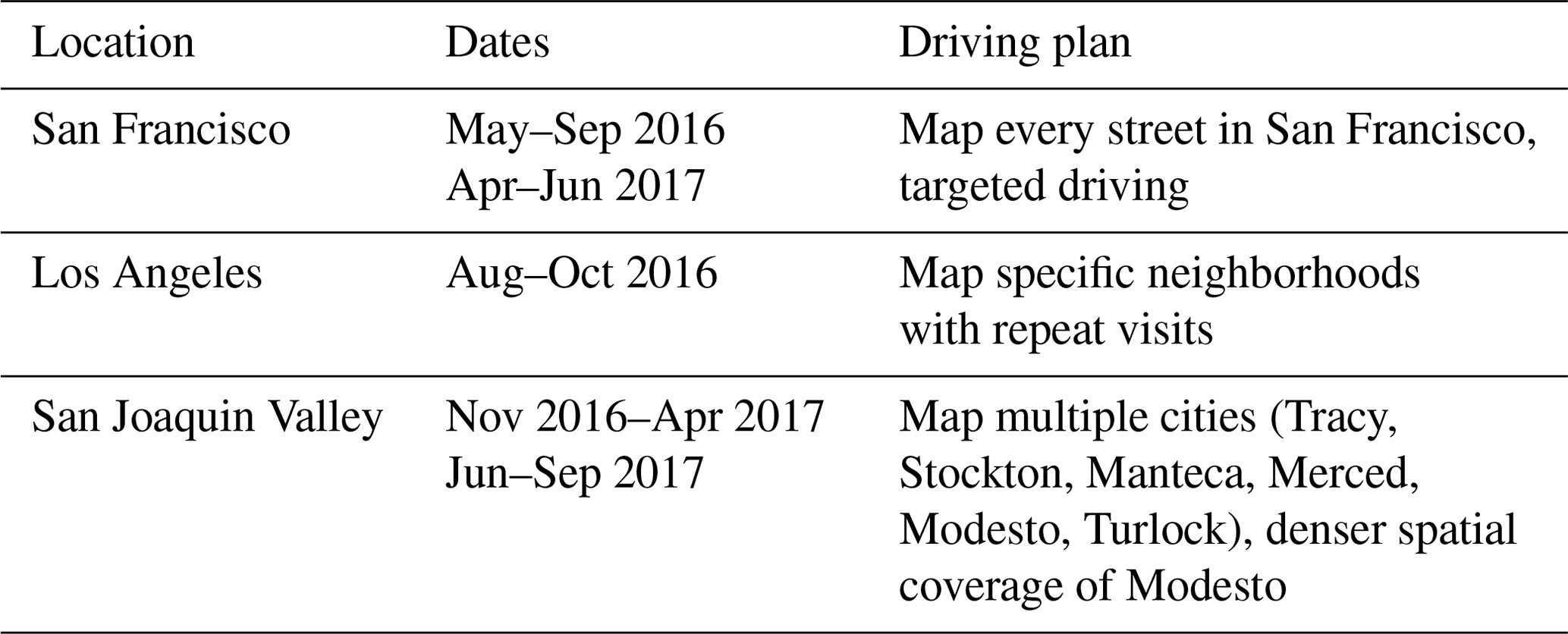
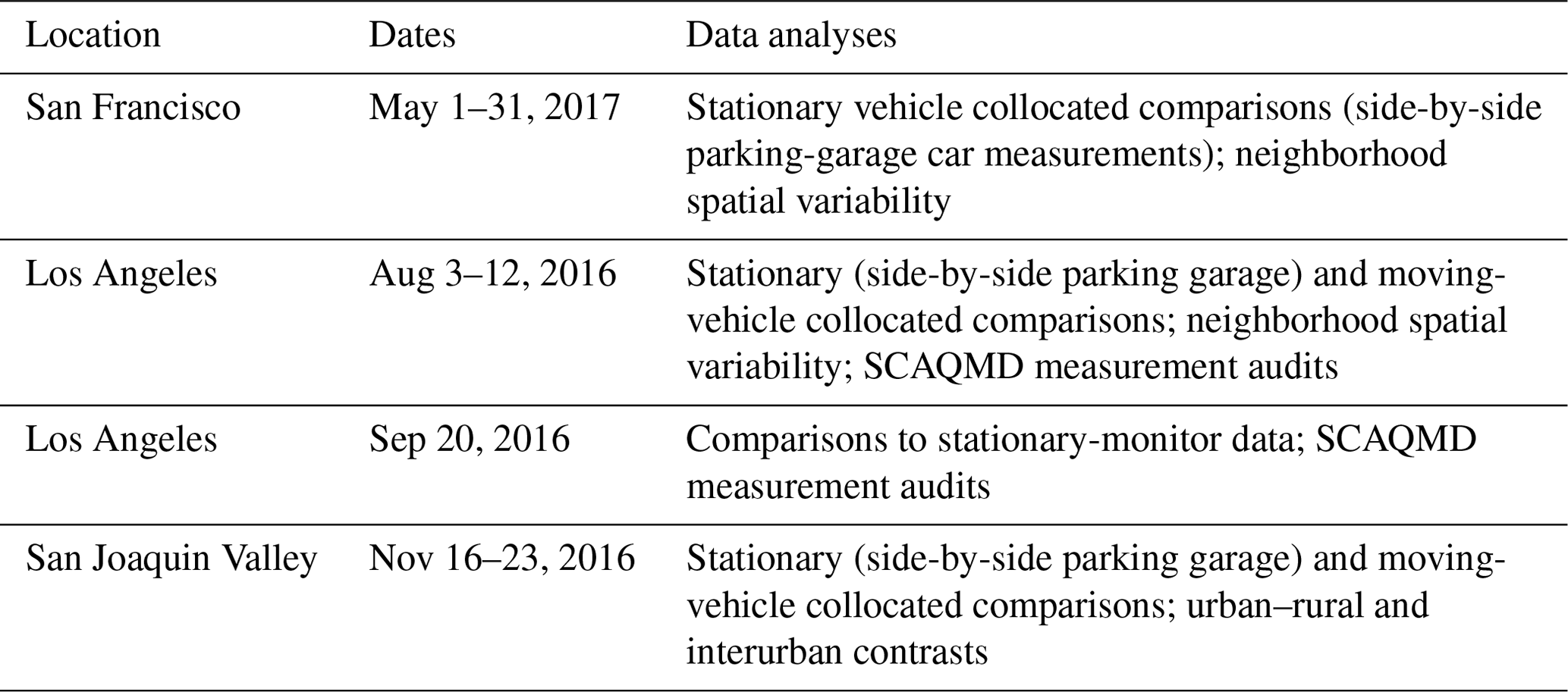
Table 2 Data sets used to evaluate spatial variability and to address individual research questions, including measurement uncertainty.

Street-level sampling was conducted in three California locations: San Francisco, Los Angeles, and smaller cities and nonurban areas within the northern San Joaquin Valley (Table 1). Measurements were made between ∼09:00 and ∼17:00 LT on weekdays, with additional sampling occurring while the vehicles were parked in the San Francisco garage and a small (∼30 car) Los Angeles parking lot before (∼06:00–09:00 LT) and after (∼17:00–22:00 LT) the driving periods. The instruments were switched from vehicle to line power when parked overnight. The vehicles were parked in dedicated areas away from traffic within each overnight parking location. Specific time periods were selected for analysis to represent data from different areas and to address individual research questions (Table 2). The selected periods do not represent the full set of driving routes in any of the areas but are instead intended to address the research objectives in Table 2, as discussed in Sect. 3. Driving routes were mapped for visualization (Supplement). For clarity, data are labeled by car names (Coltrane, Flora, Rhodes; these names do not duplicate the names of any stationary monitors).

Table 3 Sampling locations and dates for calibrations and audits through sample inlets conducted adjacent to stationary air quality monitors in Los Angeles. Date format is as follows: mm/dd/yyyy.

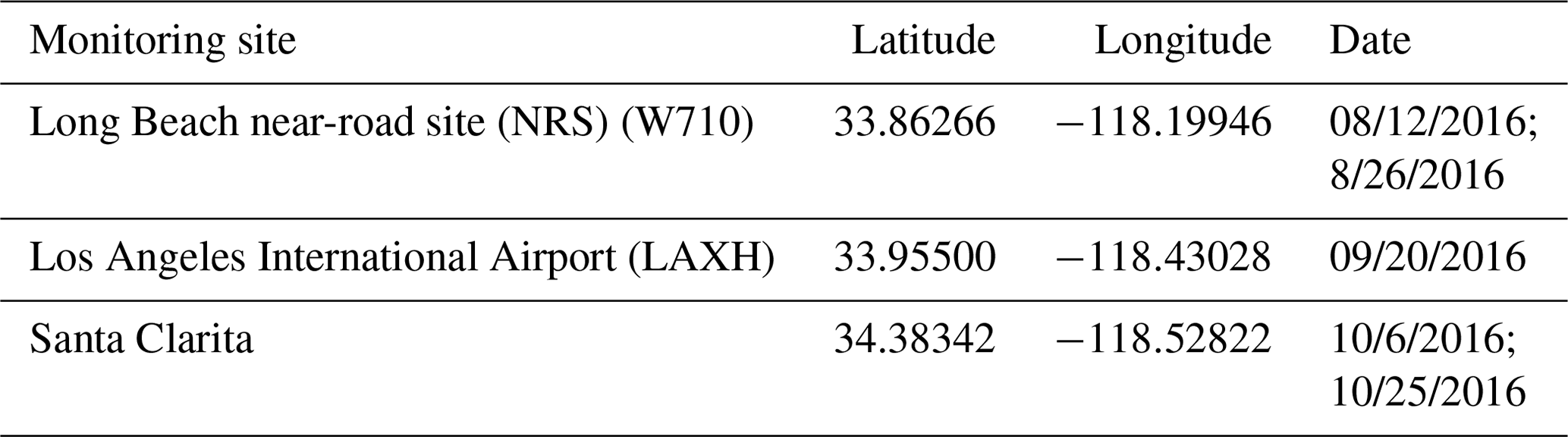
Table 4 Stationary monitoring sites in Los Angeles for which the SCAQMD provided high-resolution (1 min) measurements. Hourly average gas and PM_2.5 mass concentrations are available for other locations through EPA public data archives.

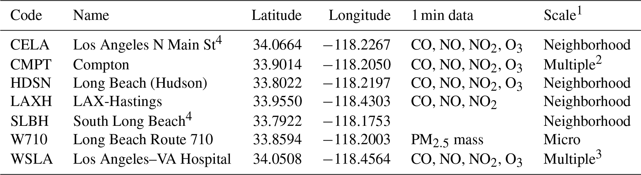
¹ EPA scales of representation are documented in Appendix D to Part 58 – Network Design Criteria for Ambient Air Quality Monitoring (https://www.law.cornell.edu/cfr/text/40/appendix-D_to_part_58, last access: 15 April 2020). Neighborhood scale is 0.5 to 4 km, middle scale is 100 m to 0.5 km, and micro-scale is several meters to ∼100 m. ² Neighborhood scale for O₃; middle scale for other species. ³ Middle scale for NO₂; neighborhood scale for O₃. ⁴ Hourly PM_2.5 or PM₁₀ measurements available.

During the Los Angeles sampling, the South Coast Air Quality Management District (SCAQMD) conducted through-the-inlet audits and calibration checks when the sampling vehicles were parked adjacent to stationary air quality monitoring sites (Table 3). The SCAQMD also prepared 1 min resolution data files for measurements made at these and other stationary air quality monitoring sites (Table 4; see also location map in Fig. S1 in the Supplement). Data from one of the dates and locations (LAXH, 20 September 2016) were suitable for collocated comparison with mobile measurements (Table 3). The stationary-monitor data from W710 consisted only of 1 h resolution PM_2.5 mass (Table 4), which was not measured by the mobile platforms, and no data were provided for the Santa Clarita site (Table 3).

The Aclima mobile measurement and data integration platform consists of fast-response (< 1 to 8 s), research-grade analyzers providing data at 1 s (1 Hz) resolution. Details about the measurement techniques along with manufacturer specifications are provided in Table S1 in the Supplement (see also Lunden and LaFranchi, 2017). The inlet and sampling manifolds were designed to minimize self-sampling as well as particle- and gas-phase sample losses. Separate inlet lines were used for particles (copper) and gases (Teflon™, a brand name of polytetrafluoroethylene). The gas-phase inlet line was set to a 90^∘ angle to the direction of traffic, and the particle and black carbon (BC) sampling inlet line faced forward. BC was measured using a photoacoustic extinctiometer, nitric oxide (NO) was measured using chemiluminescence, nitrogen dioxide (NO₂) was measured using cavity-attenuation phase-shift spectroscopy, ozone (O₃) was measured using ultraviolet (UV) absorption, and methane (CH₄) was measured using off-axis integrated cavity output spectrometry. Particle number (PN) concentration was measured using an optical particle counter, with particle counts per liter (c L⁻¹) reported in five size ranges: 0.3 to 0.5 µm (PN_0.3–0.5), 0.5 to 0.7 µm (PN_0.5–0.7), 0.7 to 1.0 µm (PN_0.7–1.0), 1.0 to 1.5 µm (PN_1.0–1.5), and 1.5 to 2.5 µm (PN_1.5–2.5).

To ensure that the 1 Hz measurements did not drift in time, on-board computers were synchronized throughout the day using Network Time Protocol (NTP), which synchronizes computers to coordinated universal time (UTC) with accuracies on the order of milliseconds. Each car recorded time using NTP, and times were reported to the nearest second in UTC. Timestamps were adjusted to account for residence time in the tubing and instrument response as described in Apte et al. (2017). We used time series plots to check the temporal comparability of vehicle and stationary-monitor measurements at 1 min resolution (Sect. 3.3).

The gas-phase instruments received zero air and span gas weekly except for CH₄, which was checked weekly at a single concentration (2020 ppbv). Performance for the gas-phase measurements is expressed as bias and precision, defined according to the Data Quality Assessment guidelines used by the United States Environmental Protection Agency (US EPA) (Camalier et al., 2007). For O₃, NO, and NO₂, the guideline analysis yields relative (in %) and absolute (in ppbv) contributions to uncertainties (Table 5). For CH₄, the analysis yields an absolute uncertainty for bias and precision of 66.7 ppbv (3.3 %), based on reference measurements at 2020 ppb.

Additional uncertainties, which range from 1 % to 3.6 %, are associated with the accuracy of the calibration gas standards and the gas delivery and generation system. Field sampling uncertainties are discussed later.

Table 5 Performance summary of the gas-phase instruments (NO, NO₂, O₃, and CH₄) in parked vehicles (Lunden and LaFranchi, 2017). n/a: not applicable

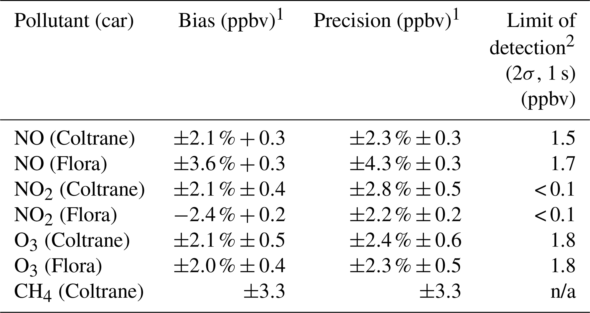
¹ Bias and precision are expressed as the upper bounds (at 90 % confidence) of bias and precision metrics determined from differences between measured and target (audit) concentrations (Camalier et al., 2007). ² Limit of detection (LOD) is defined as the minimum concentration at which an observation can be discriminated from zero (with 95 % confidence) at the specified sampling frequency (2 standard deviations of zero gas measurements).

Table 6 Performance of particle instruments (PN and BC) based on collocated parked vehicles. Evaluations performed between May 2016 and August 2017 (Lunden and LaFranchi, 2017).

¹ Bias for PN is calculated according to Camalier et al. (2007), where the values obtained by one car (Car A) are substituted for target (audit) concentrations. The positive sign of the bias estimate for the PN_1.0–2.5 (c L⁻¹) indicates a tendency of one instrument (Car B) to be biased high relative to the other instrument (Car A). Because BC concentrations were often close to LOD, bias for BC was estimated from linear least-squares regression of bias vs concentration. A single bias value was estimated for each 6 h collocation period using 1 min aggregations from two vehicles. The bias estimates were regressed against the mean concentrations measured for the corresponding times. The relative and absolute components of bias were identified from the slope and intercept, respectively, of this linear regression (r²=0.37, p value < 0.0001). ² Precision is calculated according to Camalier et al. (2007), where the mean concentrations obtained by two cars are substituted for target (audit) concentrations. ³ PN root-mean-square error (RMSE) is determined from the vehicles' PN concentration differences relative to the means of the PN measured by the vehicles. RMSE for BC is estimated through a linear regression method (RMSE vs concentration) analogous to the procedure for estimating BC bias.

The performance of the BC and PN instruments was evaluated from collocated parked vehicles (approximately weekly for PN and nightly for BC), since certified reference standards are not available for BC and PN. Both PN and BC instruments were periodically returned to their respective manufacturers, typically once per year or when the results of ambient collocations indicated substantial drift of one car relative to the other(s) or other diagnostic checks indicated that service was required. Table 6 shows the results of evaluations performed between May 2016 and August 2017.

We calculate the BC limit of detection (LOD; see footnote 2 – Table 5) using data reported while the instrument is performing an internal zero, which occurs every 10 min for 60 s. This value is typically in the range of 0.2–0.3 µg m⁻³ for the 1 Hz data while the cars are parked. For vehicles in motion, we estimate 1 Hz LOD values of 0.4 µg m⁻³ for vehicle speeds less than 5 m s⁻¹ and 0.8 µg m⁻³ for vehicle speeds greater than 5 m s⁻¹.

2.2 Location uncertainty

Location uncertainty was determined as the variability in recorded positions when vehicles were parked overnight. The vehicles did not necessarily return to the same spaces within the designated Aclima parking area each night. Therefore, variances and standard deviations of parked-vehicle east–west and north–south GPS locations were determined by vehicle, date, and time of day (i.e., before and after each daily drive). Composite east–west and north–south standard deviations were then determined from individual variances weighted by sample numbers. Composite variances were converted to location uncertainty (twice the square root of the sum of the east–west and north–south composite variances). The observed 2σ location uncertainty for vehicles parked in the San Francisco parking structure was ±6.0 m, comparable to the GPS manufacturer specifications (5 m). The location uncertainties for vehicles parked in the Los Angeles parking lot were larger (±12.2 m at 1 s resolution and ±11.5 m for 1 min averages). The GPS location uncertainties therefore impose inherent limits to the spatial resolution of the data on the order of 10 m.

2.3 Comparisons between measurement platforms

For ambient comparisons between vehicles or between vehicles and stationary monitors, our approach for computing comparability necessarily differs from EPA guidelines for determining precision and bias, which require testing against analytical standards. Because neither vehicle nor stationary-monitor measurements are analytical standards, comparability must be determined in terms of the differences between measurements made by different vehicles or between vehicle and stationary-site data, which yields instrument-to-instrument comparability. Data files were merged by 1 s or 1 min resolution times and were then used to determine time-matched paired differences, which were evaluated as functions of ambient concentration, intervehicle distance, and vehicle speed. Paired differences were evaluated for bias of one measurement relative to another. The variabilities in the paired differences relative to the means of the paired differences were also calculated. The computational approach was necessarily limited to parameters that were measured on each of two platforms (e.g., two cars or one car plus one stationary monitor). BC and CH₄ were each measured by only one vehicle while operating (during drives, one vehicle was equipped with a BC sampler and the other with a CH₄ instrument). Therefore, it was not possible to compare BC or CH₄ concentrations between operational vehicles. As previously noted, however, BC and CH₄ instruments were each installed on multiple vehicles and used to establish parked-vehicle instrument-to-instrument bias and precision: two vehicles were used in this study and two used by Apte et al. (2017), but all four vehicles were parked in the same San Francisco garage. BC and CH₄ data were not available from stationary monitors.

2.4 Statistical metrics

Various statistical metrics were computed to evaluate the comparability of time-paired measurements between vehicles or between vehicles and stationary monitors. These metrics include mean differences and fractional (relative) mean differences:

$$\begin{array}{}\text{(1)}& \begin{array}{rl}\text{Mean Difference}& \left(\mathrm{MD}\right)={\mathit{\mu }}_{\text{A-B}}=\text{mean}(X_{\mathrm{A}}-X_{\mathrm{B}}{)}_i\\ & =\text{Mean Difference}(\text{Car A}-\text{Car B}),\end{array}\end{array}$$

where σ_A-B is the standard error (SE) of the mean of (X_A–X_B)_i, “i” denotes the “ith” measurement of n paired measurements, SE is $(\surd n{)}^{-\mathrm{1}}\times$ standard deviation of (X_A–X_B), and

$$\begin{array}{}\text{(2)}& \begin{array}{rl}\text{Fractional (relative)}& \text{Mean Difference (FMD)}\\ & ={\mathit{\mu }}_{\text{A-B}}/{\mathit{\mu }}_{\mathrm{AB}},\end{array}\end{array}$$

is the mean difference (Car A – Car B) / mean of Car A and Car B mean concentrations, ${\mathit{\sigma }}_{\mathrm{FMD}}^{\mathrm{2}}=\mathit{\left\{}\right({\mathit{\sigma }}_{\text{A-B}}/{\mathit{\mu }}_{\mathrm{AB}}{)}^{\mathrm{2}}+({\mathit{\sigma }}_{\mathrm{AB}}\times {\mathit{\mu }}_{\text{A-B}}/{\mathit{\mu }}_{\mathrm{AB}}^{\mathrm{2}}{)}^{\mathrm{2}}\mathit{\}}={\mathrm{FMD}}^{\mathrm{2}}\times \mathit{\left\{}\right({\mathit{\sigma }}_{\text{A-B}}/{\mathit{\mu }}_{\text{A-B}}{)}^{\mathrm{2}}+({\mathit{\sigma }}_{\mathrm{AB}}/{\mathit{\mu }}_{\mathrm{AB}}{)}^{\mathrm{2}}\mathit{\}}$, where μ_A-B= mean(X_A–X_B )_i and σ_A-B= standard error (SE) of the mean (X_A–X_B )_i, ${\mathit{\mu }}_{\mathrm{AB}}=\mathit{\left\{}\right(\mathrm{1}/\mathrm{2})\times ({\mathit{\mu }}_{\mathrm{A}}+{\mathit{\mu }}_{\mathrm{B}}\left)\mathit{\right\}}$ and ${\mathit{\sigma }}_{\mathrm{AB}}^{\mathrm{2}}=\mathit{\left\{}\right(\mathrm{1}/\mathrm{4})\times ({\mathit{\sigma }}_{\mathrm{A}}^{\mathrm{2}}+{\mathit{\sigma }}_{\mathrm{B}}^{\mathrm{2}}\left)\mathit{\right\}}$,

$$\begin{array}{}\text{(3)}& \begin{array}{rl}\text{Fractional Absolute}& \text{Mean Difference (FAMD)}\\ & =\left|{\mathit{\mu }}_{\text{A-B}}\right|/{\mathit{\mu }}_{\mathrm{AB}},\end{array}\end{array}$$

$=|$ Mean Difference (Car A–Car B)| / Mean of Car A and Car B Mean Concentrations, ${\mathit{\sigma }}_{\mathrm{FAMD}}^{\mathrm{2}}={\mathrm{FAMD}}^{\mathrm{2}}\times \mathit{\left\{}\right({\mathit{\sigma }}_{\text{A-B}}/{\mathit{\mu }}_{\text{A-B}}{)}^{\mathrm{2}}+({\mathit{\sigma }}_{\mathrm{AB}}/{\mathit{\mu }}_{\mathrm{AB}}{)}^{\mathrm{2}}\mathit{\}}$, where ${\mathit{\mu }}_{\text{A-B}}=\mathrm{mean}(X_{\mathrm{A}}-X_{\mathrm{B}}{)}_i$ and ${\mathit{\sigma }}_{\text{A-B}}=\mathrm{SE}(X_{\mathrm{A}}-X_{\mathrm{B}}{)}_i$ and ${\mathit{\mu }}_{\mathrm{AB}}=\mathit{\left\{}\right(\mathrm{1}/\mathrm{2})\times ({\mathit{\mu }}_{\mathrm{A}}+{\mathit{\mu }}_{\mathrm{B}}\left)\mathit{\right\}}$ and ${\mathit{\sigma }}_{\mathrm{AB}}^{\mathrm{2}}=\mathit{\left\{}\right(\mathrm{1}/\mathrm{4})\times ({\mathit{\sigma }}_{\mathrm{A}}^{\mathrm{2}}+{\mathit{\sigma }}_{\mathrm{B}}^{\mathrm{2}}\left)\mathit{\right\}}$, and the following equation,

$$\begin{array}{}\text{(4)}& \begin{array}{rl}\text{Fractional Mean}& \text{Absolute Difference}=\mathrm{FMAD}\\ & ={\mathit{\mu }}_{\mathrm{|}A-B\mathrm{|}},/{\mathit{\mu }}_{AB}\end{array}\end{array}$$

= Mean Difference | Car A–Car B |/Mean of Car A and Car B Mean Concentrations ${\mathit{\sigma }}_{\mathrm{FMAD}}^{\mathrm{2}}={\mathrm{FMAD}}^{\mathrm{2}}\times \mathit{\left\{}\right({\mathit{\sigma }}_{\mathrm{|}A-B\mathrm{|}}/{\mathit{\mu }}_{\mathrm{|}A-B\mathrm{|}}{)}^{\mathrm{2}}+({\mathit{\sigma }}_{\mathrm{AB}}/{\mathit{\mu }}_{\mathrm{AB}}{)}^{\mathrm{2}}\mathit{\}}$, where ${\mathit{\mu }}_{\text{A-B}}=\mathrm{mean}|X_{\mathrm{A}}-X_{\mathrm{B}}{|}_i$ and ${\mathit{\sigma }}_{\text{A-B}}=SE|X_{\mathrm{A}}-X_{\mathrm{B}}{|}_i$ and ${\mathit{\mu }}_{\mathrm{AB}}=\mathit{\left\{}\right(\mathrm{1}/\mathrm{2})\times ({\mathit{\mu }}_{\mathrm{A}}+{\mathit{\mu }}_{\mathrm{B}}\left)\mathit{\right\}}$ and ${\mathit{\sigma }}_{\mathrm{AB}}^{\mathrm{2}}=\mathit{\left\{}\right(\mathrm{1}/\mathrm{4})\times ({\mathit{\sigma }}_{\mathrm{A}}^{\mathrm{2}}+{\mathit{\sigma }}_{\mathrm{B}}^{\mathrm{2}}\left)\mathit{\right\}}$.

The variances ${\mathit{\sigma }}_{\mathrm{FMD}}^{\mathrm{2}}$, ${\mathit{\sigma }}_{\mathrm{FAMD}}^{\mathrm{2}}$, and ${\mathit{\sigma }}_{\mathrm{FMAD}}^{\mathrm{2}}$ are derived from standard formulae for propagating errors (Caldwell and Vahidsafa, 2019; Goodman, 1960; Ku, 1966). Standard errors are the appropriate measure of the variability in mean concentrations and differences, such as those defined here, whereas standard deviations are appropriately used to quantify the variability in individual measurements (see Sect. 3, “Results and discussion”).

The preceding equations, while expressed as car-to-car comparisons, are readily applied to other comparisons, e.g., vehicle-to-stationary monitor. If one measurement (e.g., measurement A) is defined as a reference standard, then the term μ_AB in the denominator of the expressions for fractional mean difference (FMD), fractional absolute mean difference (FAMD), and fractional mean absolute difference (FMAD) may be appropriately replaced by the reference mean (μ_A). Mean differences are used when absolute comparisons (i.e., retaining concentration units) are informative. Fractional differences are useful for establishing vehicle-to-vehicle or vehicle-to-monitor differences relative to the magnitudes of the mean concentrations.

The FMD retains its sign and therefore indicates if μ_A > μ_B. This metric is useful when the sign is important for identifying which instrument (e.g., mobile or stationary) or which location records higher concentrations. The FAMD and FMAD are useful if the sign of the difference is not meaningful. The sign is usually not relevant, for example, in the analysis of intervehicle measurement differences as a function of the distance between the vehicles (“Results and discussion”), in which the objective is to characterize the rate at which measurement comparability decays with distance. The FAMD is simply the absolute value of the FMD, and both metrics approach zero when individual paired measurement differences tend to average out over a set of samples. In contrast, the FMAD provides a measure of the variability in individual measurements because it averages absolute values of concentrations. The FMAD is relevant to understanding the comparability of high-resolution (e.g., 1 s) measurements, whereas the FAMD is a measure of the comparability of a time or space average determined from individual measurements.

Performance audits (Tables 5 and 6) indicate that fractional differences (FAMDs) exceeding ∼0.1 (10 %) for gases and ∼0.2 (20 %) for PN are, in general, likely to be physically meaningful relative to measurement uncertainties (bias and precision are each < 5 % for gases at concentrations > 2–24 ppbv; 7 %–26 % for PN and BC). Only the two largest PN size ranges exhibit bias exceeding 20 % (Table 6). Combining bias and precision indicates a total uncertainty of ∼10 % for gases and ∼20 % for PN_0.3–0.5. In operation, the comparability of measurements made in moving vehicles differs from those made in parked collocated vehicles (see “Results and discussion”), so we utilize a higher threshold (i.e., 20 %) for establishing true spatial variations even for gas-phase species.

Table 7 Mean ambient concentrations and sample sizes as measured by the mobile platforms in each of the example study areas.¹ NA: not available.

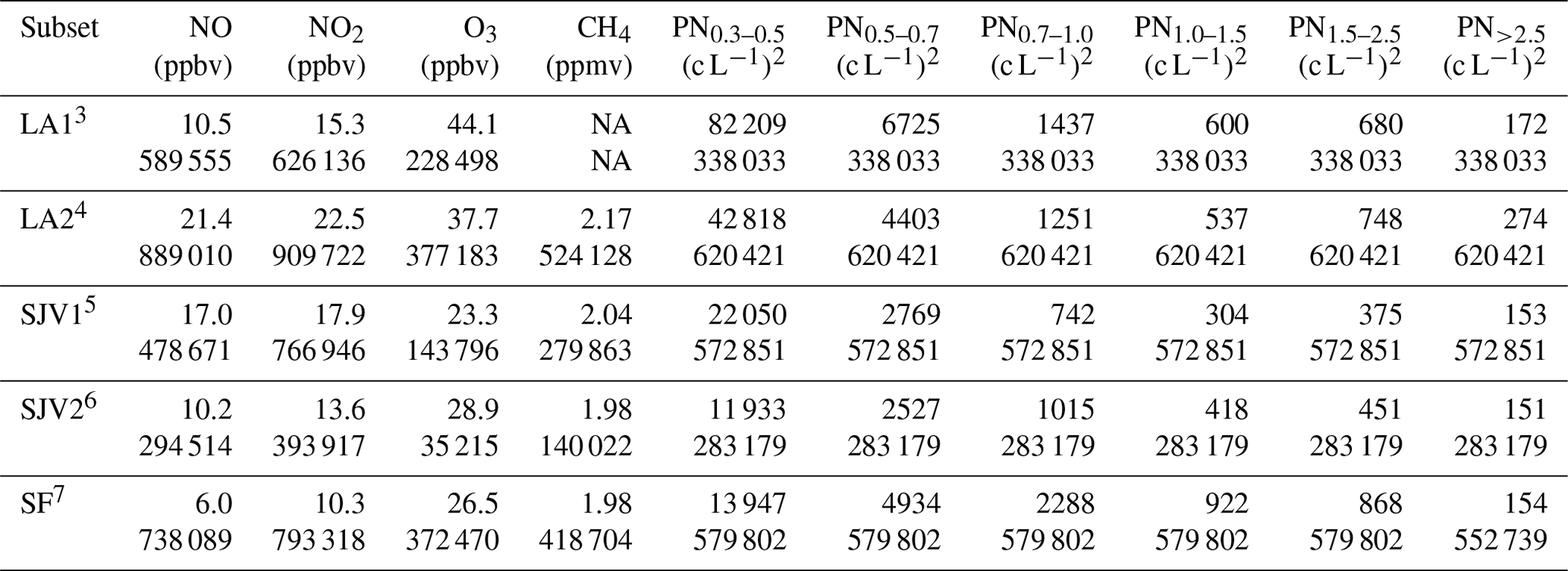
¹ Sample sizes are total number of 1 s measurements summed across vehicles. Means are weighted by the number of measurements per vehicle. ² Particle number in size fractions 0.3–0.5, 0.5–0.7, 0.7–1.0, 1.0–1.5, 1.5–2.5, and > 2.5 µm. ³ LA1 is Los Angeles, 3–12 August 2016 (8 d). BC and CH₄=1 car; NO, O₃, NO₂, and PN =2 cars. ⁴ LA2 is Los Angeles, 12–30 September 2016 (14 d). BC and CH₄=1 car; NO, O₃, NO₂, and PN =2 cars. ⁵ SJV1 is San Joaquin Valley, 16–23 November 2016 (6 d). BC and CH₄=1 car, NO and O₃=2 cars, and NO₂ and PN =3 cars. ⁶ SJV2 is San Joaquin Valley, 20–29 March 2017 (6 d). BC and CH₄=1 car, NO and O₃=2 cars, NO₂ and PN =2 cars. ⁷ SF is San Francisco, 1–12 May 2017 (10 d). BC and CH₄=1 car; NO, O₃, NO₂, and PN =2 cars.

3 Results and discussion

Mean concentrations during example study periods are summarized in Table 7 for context. Subsequent analyses of spatial heterogeneity, which are presented in later subsections and depend on the availability of measurements from two or more sampling platforms, focus on NO, NO₂, O₃, and PN_0.3–0.5. These pollutants are of interest because they are measured with differing accuracies, they exhibit differing degrees of spatial variation, and they vary in their degree of atmospheric chemical processing. NO is a primary pollutant, and NO₂ forms rapidly (i.e., minutes) from NO. NO₂ formation and O₃ loss are linked through the rapid reaction of NO with O₃ to form NO₂; Seinfeld and Pandis (2016) calculate a 1∕e lifetime for NO of 42 s at 50 ppb O₃. O₃ formation and accumulation occur more slowly (i.e., hours) from NO₂ and volatile organic compounds (VOCs) in the presence of UV radiation (Seinfeld and Pandis, 2016). PN_0.3–0.5 is the smallest size fraction that was measured, present in the highest numbers (83 % of PN; Table 7), and is likely indicative of newly aged particles from fresh motor-vehicle emissions (Zhang and Wexler, 2004; Zhang et al., 2004; Zhu et al., 2002).

The fraction of PN in the 0.3–0.5 µm size fraction was lower in spring (60 % in San Francisco, May 2017, and 72 % in the San Joaquin Valley, March 2017) and higher in summer (90 % in Los Angeles, August 2016) and autumn (86 % in Los Angeles, September 2016, and 84 % in the San Joaquin Valley, November 2016) (Table 7). Although these differences in the PN size distributions possibly reflect regional-scale spatial variability, no simple comparison among regions is possible due to sampling them during different seasons. The regional differences could in fact reflect seasonal variations in PM composition: the observed variations in PN distributions are consistent with past studies that indicate the importance of PM nitrate (NO₃) found in larger (> 0.5 µm) size fractions primarily as ammonium nitrate in California during cooler months (e.g., Herner et al., 2005), which could lead to the observance of different size distributions in the different regions.

Mean concentrations of gases were comparable among the study locations and periods (Table 7). O₃ concentrations were highest in Los Angeles in August near downtown (south of the CELA site; Figs. S6 and S7), followed by concentrations in September in western Los Angeles near the WSLA site (Fig. S8) and near Los Angeles airport (near the LAXH site; Fig. S3). Mean O₃ in the remaining locations (SJV and SF) falls within a narrow range (23–29 ppbv) and is only lower by a factor of less than 2 than in Los Angeles. Mean concentrations of NO₂ also vary by a factor of 2, with highest concentrations near the LA airport and lowest concentrations in SF (Table 7). Concentrations of NO are highest by a factor of about 2 in Los Angeles near the airport and in the SJV in November during mostly freeway driving. At all locations studied, typical NO–NO₂–O₃ chemistry was observed, with higher NO and NO₂ concentrations and lower O₃ levels near mobile emission sources. Mean methane concentrations were low (∼2 ppmv) during all periods and varied among areas within < 0.1 ppmv. As with PN, these average concentrations likely vary due to time of year, location relative to source emissions, and chemical processing.

Table 8 External calibration checks (zero and span) performed in Los Angeles with equipment and gas standards managed by the SCAQMD compared with internal checks performed by Aclima 1 month prior to the Los Angeles deployment, 1 month following this deployment, and during a 1-week return to San Francisco in the middle of the deployment. External and Aclima calibration checks were conducted through the inlet lines of the mobile platforms.

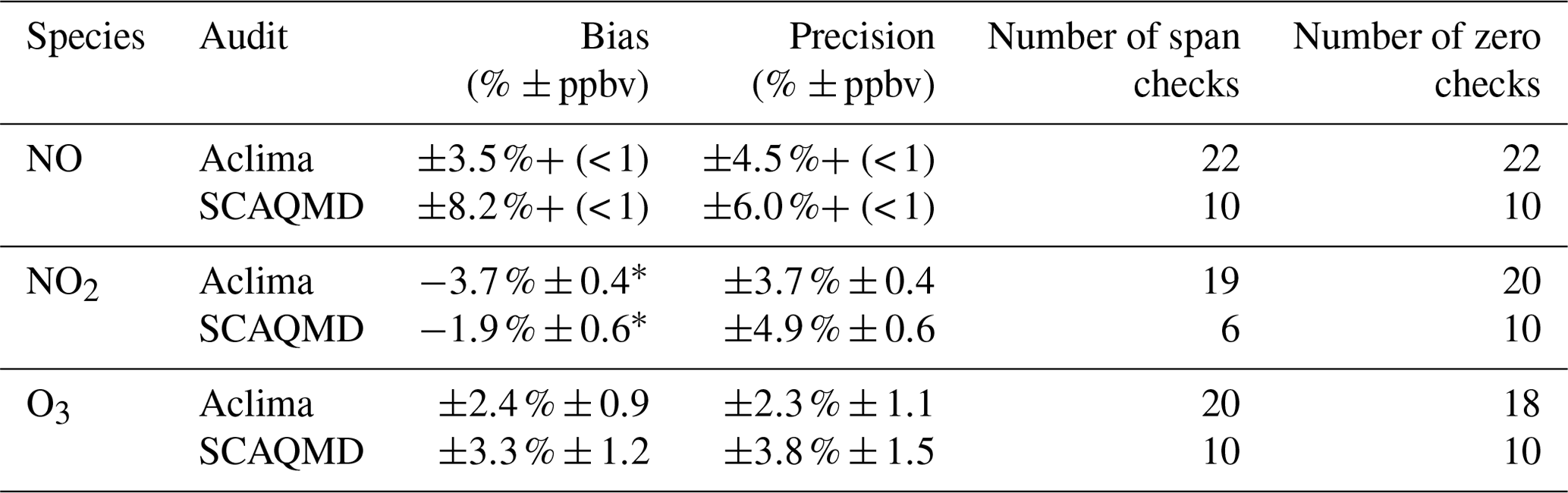
^* Negative bias only.

3.1 Comparability of measurements in the mobile platforms to the inlet audits

Field calibration checks (zero and span) were conducted through inlets using SCAQMD equipment and standards; these checks were compared with Aclima calibration checks that were made before, during, and after the period when vehicles drove in Los Angeles (Table 8). The SCAQMD and Aclima checks were comparable and indicate that measurements of the tested gas-phase species (NO, NO₂, and O₃) maintained accuracy and replicability in the field during the Los Angeles driving routes. The Los Angeles drives followed the same field protocols as the drives in San Francisco and the San Joaquin Valley. The cross-lab differences between the Aclima and SCAQMD calibration checks (defined as the lab-to-lab differences in the mean relative differences from target concentrations averaged over all calibration checks) were $-\mathrm{5}\mathit{\%}\pm \mathrm{2.0}\mathit{\%}$ for NO, $-\mathrm{1.5}\mathit{\%}\pm \mathrm{1.0}\mathit{\%}$ for NO₂, and $+\mathrm{0.5}\mathit{\%}\pm \mathrm{1.3}\mathit{\%}$ for O₃ (not tabled). All differences were less than the invalidating limits for the South Coast Air Quality Management District's weekly calibration checks: 7 % for O₃ and 10 % for CO, SO₂, and NO_x (Table 2.4; https://ww3.arb.ca.gov/aaqm/qa/pqao/repository/district_sops/south_coast/quality_assurance/qapp_criteria_pollutants.pdf, last access: 15 April 2020).

Table 9 Performance summary for measurements reported by collocated vehicles (mean difference ±1 standard deviation; mean concentrations in parentheses). Standard deviations are reported here to indicate the variability in the 1 s differences. Mean differences provide a measure of average intervehicle differences. For periods when three vehicles were driven, the largest mean difference between vehicles is listed. The signs of the mean differences are not indicated because no vehicle is an audit standard. All values were determined from 1 s time resolution data.

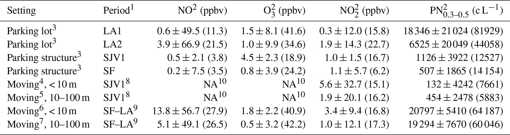
¹ LA1 is 3–12 August 2016 (8 d), LA2 is 12–30 September 2016 (14 d), SJV1 is 16–23 November 2016 (6 d), and SJV2 is 21–30 March 2017 (6 d). ² Vehicle-to-vehicle concentration differences were determined from 1 s measurements. Means and standard deviations of paired differences were determined for each data pair. Time periods when a vehicle was sampling through a calibration port (whether a calibration was in process) were excluded to ensure that vehicles were sampling the same ambient air for all comparisons. ³ The parking lot in Los Angeles was used for LA1 and LA2. The parking structure in San Francisco was used for all SF and SJV drives. ⁴ Intervehicle distance < 10 m (average =5 m); average speed =3.0 m s⁻¹ (10.6 km h⁻¹). ⁵ Intervehicle distance 10–100 m (average =32 m); average speed =25.6 m s⁻¹ (92.0 km h⁻¹). ⁶ Intervehicle distance < 10 m (average =6 m); average speed =5.9 m s⁻¹ (21.2 km h⁻¹). ⁷ Intervehicle distance 10–100 m (average =44 m); average speed =27.7 m s⁻¹ (99.7 km h⁻¹). ⁸ On 16 November 2016 (I-580 and other locations, Flora and Rhodes; Fig. S2). ⁹ On 1 August 2016 driving from San Francisco to Los Angeles (I-5 and other locations). ¹⁰ Not available. SJV1: one car (Rhodes) of collocated moving pair lacked NO and O₃ samplers.

3.2 Similarity of concentrations obtained from collocated vehicles when parked and when moving

Car-to-car comparisons were made to evaluate the comparability of collocated ambient measurements made while the vehicles were parked and while driving (Table 9). The cars generally followed different routes, as discussed later; when the cars traveled a route segment together, they drove “caravan style”, keeping each other in sight but not following immediately behind each other. Time-synchronous measurement differences reflect a combination of instrument and ambient sampling uncertainties; for moving vehicles, differences may also reflect spatial variability, depending on measurement integration times relative to intervehicle distances. The comparisons are expressed as mean car-to-car differences ±1 standard deviation of the paired 1 s differences, yielding metrics for car-to-car measurement bias and variability, respectively, averaged over ∼1000–50 000 paired differences.

The observed mean paired differences between parked vehicle measurements were 0.2–3.9 ppbv for NO, 0.3–1.9 ppbv for NO₂, and 0.8–4.5 ppbv for O₃ (Table 9). The corresponding FAMD values (absolute values of mean differences divided by mean concentrations) range from 0.03 to 0.24 (3 % to 24 %) for gases and 0.04 to 0.22 (4 % to 22 %) for PN. These differences are comparable to, or larger than, instrumental bias and precision (< 5 % each for gases at concentrations > 2–6 ppbv – Table 5; 10–11 % for PN_0.3–0.5 – Table 6). For gases and PN, the variabilities (standard deviations) in the 1 s paired differences exceed the mean differences (except O₃ during the SJV sampling period of 16–23 November 2016), which is expected because instrumental variations average toward zero when instruments are unbiased with respect to each other. The mean paired differences varied among individual sampling days (Fig. S2). Between-vehicle 1 s variability is higher in closely spaced moving vehicles than in stationary vehicles, especially for NO₂ (Table 9; note that this comparison could not be made for NO). We interpret this difference as indicating that moving vehicles sampled heterogenous parcels of air, and the intervehicle measurement differences are thus due to fine-scale spatial variability.

3.3 Similarity of mobile concentrations to stationary-monitor data

For field comparisons to stationary monitors, we worked with SCAQMD staff who operate the monitors and are familiar with all measurements made at each location. On 20 September 2016, two sampling cars parked next to the monitor at LAXH (Tables 3 and 4; Figs. S3 and S4). Relative to the ground-level position of the stationary-monitor probe (located inside a fenced enclosure), the vehicles alternated positions, from closer when audited (Coltrane – 6.6 m from LAXH; Flora – 8.5 m from LAXH) to further when sampling (Coltrane – 24.1 m for 1 h; Flora – 18.5 m for 2 h), as determined from GPS coordinates for the monitor and vehicles. The heights of the LAXH instrument probes are 4.2 m a.g.l. (meters above ground level; SCAQMD, 2018a), whereas the mobile sampler inlet heights are 2 m a.g.l.. The monitoring instruments at LAXH are in a vacant field north of Los Angeles International Airport (Fig. S4). The site is surrounded by several schools to the NE, N, and NW, with residential communities (Playa Del Rey and Westchester) north of the airport and further away surrounding the site. The closest communities include homes and two-story to four-story apartments. Minimal traffic is expected immediately adjacent to the site.

Table 10 Comparison of mobile-platform to collocated stationary-site measurements made at LAXH on 20 September 2016. The two cars alternated positions between an audit location at 6.6 m, for Coltrane, and 8.5 m, for Flora, horizontal distance from the ground-level coordinates of the LAXH monitor (inlet situated 4.2 m a.g.l. inside a fenced enclosure) and a sampling location further from the monitor (24.1 m for Coltrane and 18.5 m for Flora). Data from the audit tests are excluded. The Coltrane audit period was 10:22–00:20 PDT (n=119). The Flora audit period was 09:19–22:20 PDT (n=56). The means ± standard errors of the means were determined for each car from the 1 min measurements made at the two distances from the stationary monitor. Standard errors indicate the uncertainties of the mean concentrations and mean differences. Differences of 1 min measurements were determined prior to averaging. The variabilities in the 1 min differences can be obtained by multiplying standard errors by square root of sample size (n).

¹ Total minutes. Flora audit period – 09:19–22:20 PDT (n=56), and Coltrane audit period – 10:22–00:20 PDT (n=119). Sample sizes for individual measurements may be smaller due to excluding audit values. Mean paired differences are computed only for non-audit samples. ² ${\mathrm{O}}_x={\mathrm{NO}}_{\mathrm{2}}+{\mathrm{O}}_{\mathrm{3}}$.

The mobile platforms recorded mean concentrations of NO, NO₂, O₃, and O_x ($={\mathrm{NO}}_{\mathrm{2}}+{\mathrm{O}}_{\mathrm{3}}$) that were comparable to LAXH monitor concentrations: most mean paired differences between mobile-platform and LAXH concentrations were less than 10 % of the average concentrations (Table 10). Time series of 1 min Flora, Coltrane, and LAXH measurements show agreement (Fig. S5) (mean Flora–Coltrane distances were 12.2 and 20.2 m). CH₄ is reported in motor-vehicle emissions (Nam et al., 2004), so a correlation between NO and CH₄ will usually be observed when sampling fresh automotive exhaust emissions; all NO values correlated with Coltrane CH₄ concentrations (r²=0.84 to 0.87; Flora did not report CH₄).

3.4 Differences between mobile concentrations and stationary-monitor data when the cars are not close to monitors

Spatial variation is defined by differences in time-synchronous measurements made in differing areas. To interpret the paired differences as spatial variation, rather than measurement uncertainty, we refer to the preceding analyses of instrument and sampling performance in audit tests (Tables 5 and 6) and collocated vehicles (Table 9). As previously noted, the results for measurement bias and precision (Tables 5 and 6) and for comparability of collocated vehicles (Table 9) lead us to define FAMD > 0.2 (20 %) as an indicator that spatial variations exceed measurement and sampling uncertainties. The intent of the analyses in this section is to help elucidate the spatial scales over which stationary-monitor and mobile-platform data represent ambient concentrations and to characterize spatial heterogeneity of pollutant concentrations within neighborhoods.

Because vehicles sampled different road segments on different days and at different times of day, we compiled time-synchronous differences between the concentrations measured by two cars (or cars and monitor) to remove the confounding effects of day-to-day and diurnal variability. Random differences, such as short, intermittent exposures of one car to a high-emitting vehicle or to variations in wind directions, are averaged out in the FAMD statistic. In contrast, systematic car-to-car (or car-to-monitor) differences yield higher FAMD values. Systematic differences could occur if the instrumentation in one car were biased relative to the other car (e.g., Apte et al., 2017) or to the monitor. If instrumental sources of systemic car-to-car or car-to-monitor difference can be eliminated through side-by-side sampling comparisons (Sect. 3.2 and 3.3), we can then conclude that larger FAMD values (e.g., > 0.20 % or 20 %) represent spatial heterogeneity due to the two cars sampling different neighborhoods. FAMD is also a useful metric for evaluating the spatial scale of representativeness of stationary monitors. The relationships between FAMD and vehicle–monitor or intervehicle distance, discussed below, characterize the spatial scales of pollutant heterogeneity but do not indicate which neighborhoods experienced higher pollutant concentrations. For that purpose, we examined maps (Sect. 3.4) and developed the visualization discussed in Sect. 3.5.

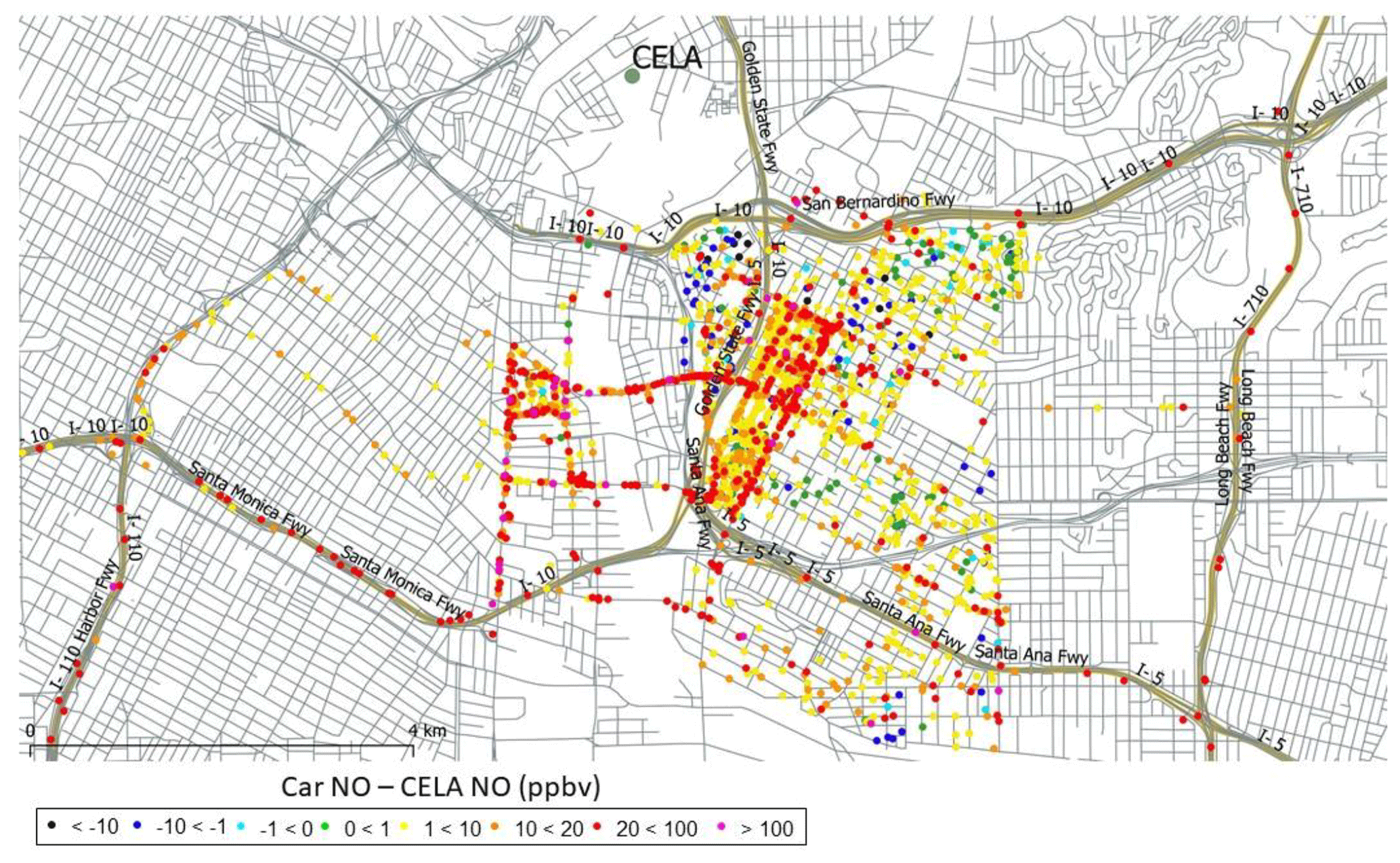
Figure 1 Paired differences in 1 min NO concentrations measured by cars and by the air quality monitor in downtown Los Angeles (CELA) during 3–12 August 2016. Map generated with QGIS version 3.2.2 (https://qgis.org/en/site/, last access: 12 June 2020) open-source software licensed under the GNU General Public License (http://www.gnu.org/licenses/licenses.html, last access: 12 June 2020). California state highway shapefiles obtained from the OpenStreetMap community (© OpenStreetMap contributors 2020, distributed under a Creative Commons BY-SA License; http://www.openstreetmap.org, last access: 12 June 2020) and MapCruzin (http://www.mapcruzin.com, last access: 12 June 2020), licensed under the Creative Commons Attribution ShareAlike 2.0 license. US highways shapefile obtained from US Bureau of the Census TIGER/Line Shapefiles public data (https://www.census.gov/geographies/mapping-files/time-series/geo/tiger-line-file.html, last access: 12 June 2020).

3.4.1 Los Angeles, August 2016

Between 3 August (the first complete Los Angeles driving day) and 12 August, the two vehicles traversed different neighborhoods south of the central Los Angeles stationary monitor (CELA; Table 4; Figs. S6 and S7) between 09:00 and 18:00 PDT at car-monitor distances ranging from 1 to 7 km. The monitoring instruments at CELA are located on a rooftop of a two-story building, and the heights of various instrument probes range from 11 to 12 m a.g.l. (SCAQMD, 2018b). Driving routes for the first sampling day (3 August) are shown in Fig. S6; most of the routes on other dates were similar. In general terms, the US 101 and one section of the I-5 freeway run across the southern border of the sampling area; the area sampled is split by a N–S portion of I-5 and bordered to the north by I-10. The I-10 freeway is situated between CELA and the measurement area. For comparison with the 1 min resolution CELA data, 1 min average concentrations were created from the 1 s mobile-platform data. Because driving speeds averaged ∼2–5 m s⁻¹, the typical distances traveled in 1 min were ∼100–300 m. The 1 min average positions of the mobile sampling are visibly discrete (Fig. S6). Differences between CELA and car 1 min concentrations were highest when cars drove along freeways but also show spatial heterogeneity within the neighborhoods sampled (Fig. 1). While in motion, generally beginning after 09:00 and ending between 17:00 and 18:00 PDT, the cars recorded higher concentrations of NO and NO₂ than the CELA stationary air monitor did, likely due to the proximity of fresh vehicle emissions experienced by street-level sampling in the vehicles (Figs. 1 and 2). During the driving hours, the vehicles recorded lower levels of O₃ than CELA did (Fig. 2). As noted in the previous comparison of collocated and stationary-monitor data, much of this difference is attributable to street-level reaction of fresh NO emissions with O₃; this interpretation is supported by the closer agreement between cars and CELA of O_x than O₃ (Fig. 2).

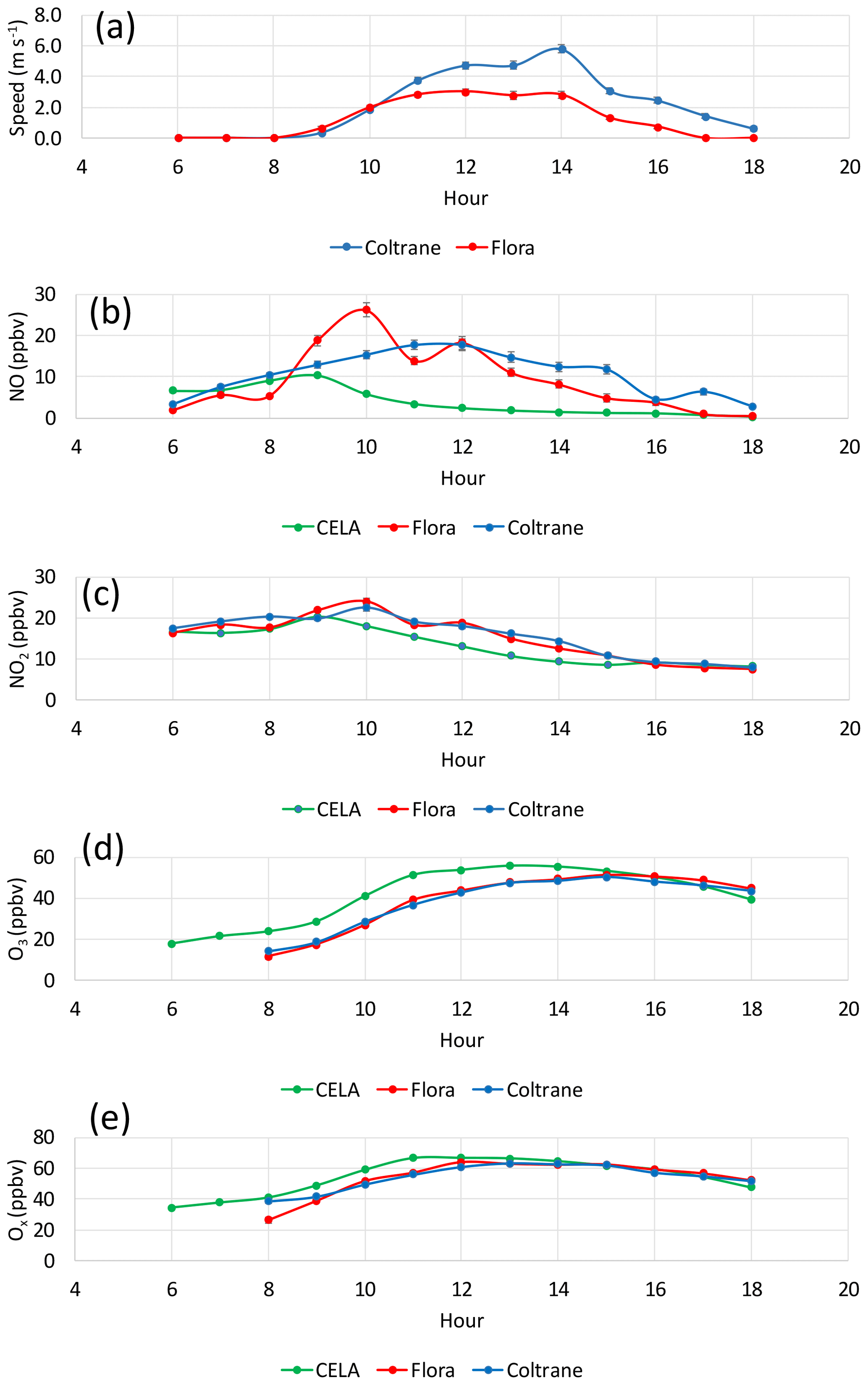
Figure 2 Mean vehicle speeds and pollutant concentrations averaged by hour over all Los Angeles driving days between 3 and 12 August 2016. Standard errors of the means are plotted but are generally smaller than the symbol sizes.

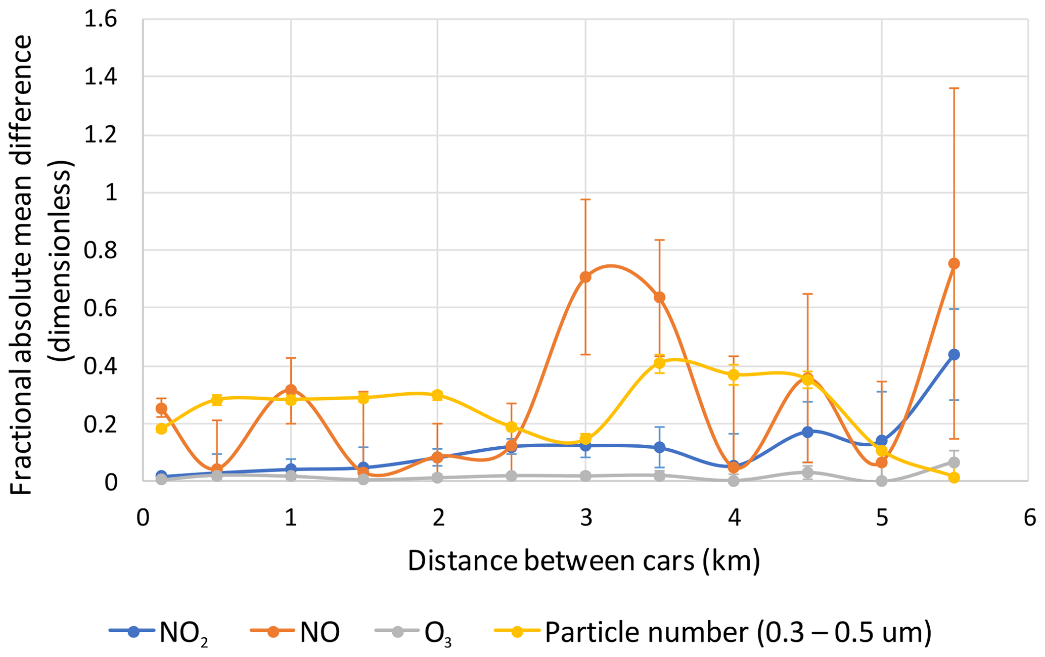
Figure 3 Intervehicle FAMD vs mean intervehicle distance associated with sampling in Los Angeles (near CELA) from 3 to 12 August, averaged over 0.5 km bins (0–0.25 km, 0.25–0.75 km, etc.). Error bars are 1σ uncertainties determined as described in the definition of FAMD. The sizes of the error bars reflect variations in the number of samples in each bin (N=14 to 2433) as well as sampling variability.

To quantify differences within and between neighborhoods, between-vehicle paired comparisons were determined as differences between time-synchronous 1 min mobile concentrations for 3–12 August (near CELA), which were then averaged over 0.5 km bins (0–0.25 km, 0.25–0.75 km, etc.) (Fig. 3). The bin-average FAMDs ranged from 0.02 (2 %) at 0.125 km to 0.14–0.44 (14 %–44 %) at 4.5–5.5 km (mean =0.12, or 12 %, over all bins) for NO₂ and from 0.006 (0.6 %) at 0.125 km to 0–0.07 (0 %–7 %) at 4.5–5.5 km (mean =0.02, or 2 %, over all bins) for O₃. For these two pollutants, the mean differences among streets and neighborhoods were therefore small (12 % and 2 %, respectively, at 0.125–5.5 km spatial scale). For NO, bin-average FAMDs were larger and ranged from 25 % at 0.125 km to 4 %–75 % at 4.5–5.5 km.

The intervehicle differences averaged over distance bins concisely summarize large numbers of measurements, but this averaging could mask finer spatial variations in possible interest. We compared the standard deviations of the mean intervehicle concentration differences to the corresponding mean concentrations to characterize variability within the spatial averages. These ratios (standard deviation of intervehicle difference / mean concentration) ranged from 0.4 to 1.0 (average =0.5) for NO₂. Within the binned intervehicle averages, therefore, vehicle-to-vehicle NO₂ concentration differences varied by up to a factor of 2 (twice the standard deviation of the mean differences) times the mean observed concentrations. For NO, the ratios ranged from 1.2 to 4.0 (average =2.8), indicating that vehicle-to-vehicle NO concentration differences varied by up to a factor of 6 (2 standard deviations) within the binned intervehicle averages.

The number of particles in the size range 0.3 to 0.5 µm exhibited FAMDs exceeding 0.2 (20 %) that were less variable than the NO FAMD. Both NO concentrations and particle numbers likely varied, as the vehicles sampled different streets and neighborhoods and experienced differing levels of fresh emissions at any given time (e.g., Figs. S6 and S7). The peak in the NO FAMD at 3 and 3.5 km corresponds to mean NO concentrations of 6.6 and 8.1 ppbv, respectively, for Flora and mean NO concentrations of 14.8 and 15.3 ppbv, respectively, for Coltrane. Many of the 85 and 120 differences of 1 min average concentrations in the 3 and 3.5 km bins, respectively, correspond to cases where Coltrane sampled close to the confluence of the Santa Anna and Golden State freeways, while Flora collected data further from freeways (Fig. S7). An approach to identifying high-concentration locations is illustrated later in the discussion of data from San Francisco (Sect. 3.5).

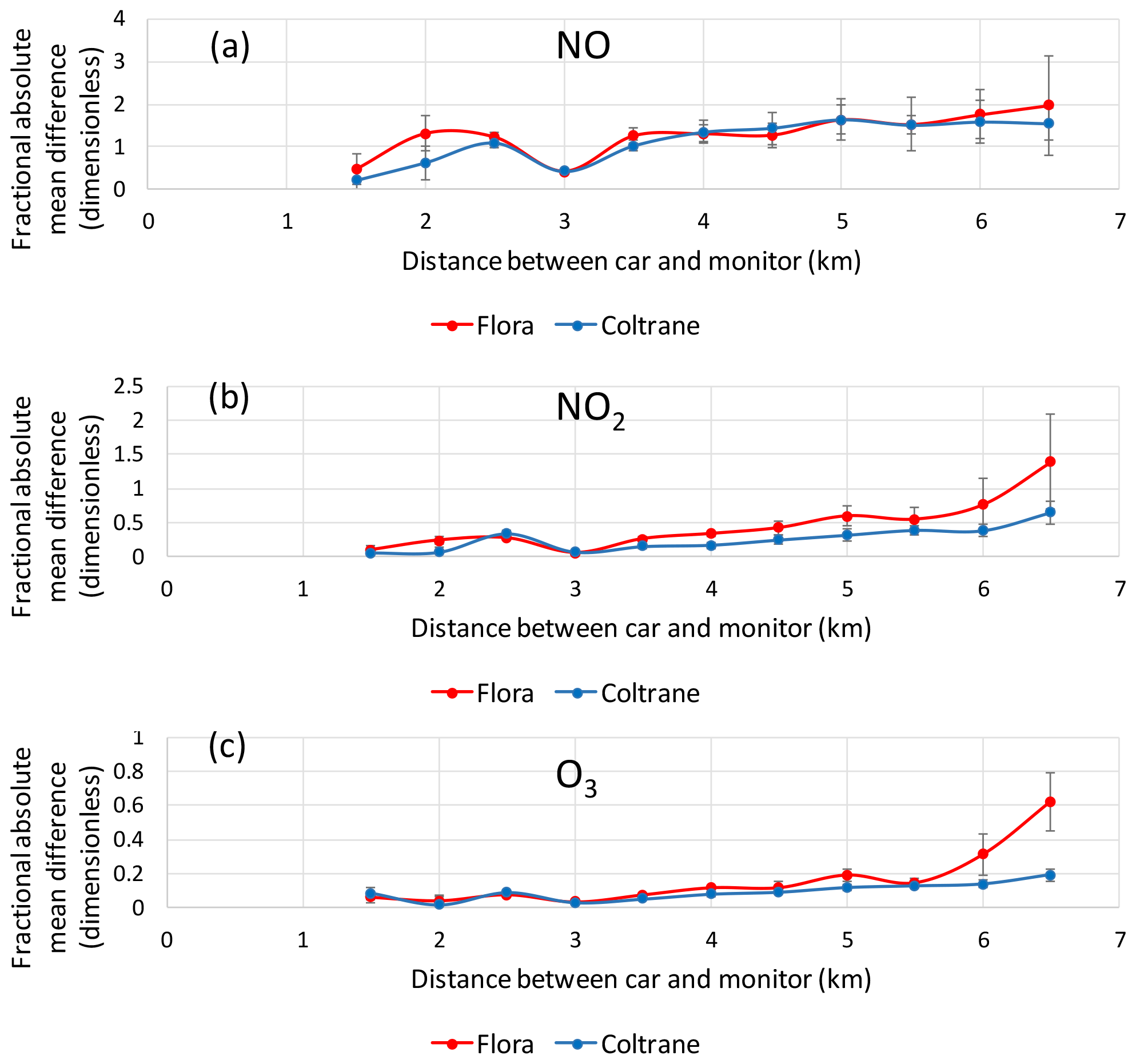
Figure 4 Fractional absolute mean difference (FAMD) for (a) NO, (b) NO₂, and (c) O₃ vs mean intervehicle distance for 3–12 August 2016, Los Angeles sampling, averaged over 0.5 km bins. Error bars are 1σ uncertainties as described in the text. The sizes of the error bars reflect variations in the number of samples in each bin (N=3–19 at 6.5 km to 222–338 at 3.5 km). The 3 km bin (N=1273–3906) consists primarily of measurements made in the parking lot.

The NO FAMD for car–CELA comparisons largely exceeded 1; the NO₂ and O₃ FAMDs were less than 0.5 and 0.2, respectively, at most car–CELA distances (Fig. 4). Although the two cars drove different routes, the two car–CELA comparisons were similar (Fig. 4). The representativeness of CELA and other sites is discussed below (Sect. 3.6).

3.4.2 Los Angeles, September 2016

Driving routes were near (< 0.2 to 5 km) the western Los Angeles stationary monitor (WSLA; Table 4) on 4 of the 14 d between 12 and 30 September (including areas shown in Fig. S8 for 13 and 19 September; similar routes were driven on 26 and 29 September). Drives began at ∼09:00 and ended by 17:00 PDT. Because only one car drove near WSLA on each of the 4 d, only car-to-WSLA comparisons are presented. The monitoring instruments at WSLA are located on the roof of a trailer on the grounds of the VA Hospital, and the heights of the instrument probes are 4.2 m a.g.l. (SCAQMD, 2018c) (Fig. S9). The monitor is located < 600 m west of I-405 and about 200 m south of a major arterial, Wilshire Boulevard. The immediate surrounding area to the north and south is grass with some trees, and slightly further out, the area is primarily residential multistory (two-story to three-story) apartment buildings.

Figure 5 Mobile-platform monitoring and WSLA measurements versus distance between cars and WSLA on 4 d (13, 19, 26, and 29 September 2016) when the cars drove near WSLA. The first bin includes all distances less than 0.5 km; the minimum distance between cars and monitor was 158 m. Locations are indicated. Standard errors of the means are shown, but most are smaller than the symbols.

The mobile platforms recorded substantially (between 70 % up to a factor of 32) higher concentrations of both NO and NO₂ than WSLA, while the cars drove from the parking garage on the Santa Monica freeway to the neighborhood destinations (Fig. 5; WSLA–car distances > 5 km). Even at distances < 0.2 km up to 5 km from WSLA, the mobile platforms recorded higher concentrations of NO and NO₂. However, mean car and WSLA O_x concentrations at distances < 10 km were more similar than corresponding car and WSLA concentrations of NO₂ and O₃ (Fig. 5). For NO and NO₂, the FAMD exceeded 1.5 and 0.4, respectively, at all distances outside the parking garage (Fig. 6). During part of their routes, the cars were sampled adjacent to the San Diego (I-405) freeway, which likely contributed to higher mean NO and NO₂ concentrations for the mobile platforms. The WSLA monitoring site (grounds of VA Hospital) has a middle-scale zone of representation (100 m to 0.5 km) for NO₂ (Table 4), consistent with our results. For O₃ and O_x, the FAMDs were < 0.2 and < 0.05, respectively, within 5 km of WSLA.

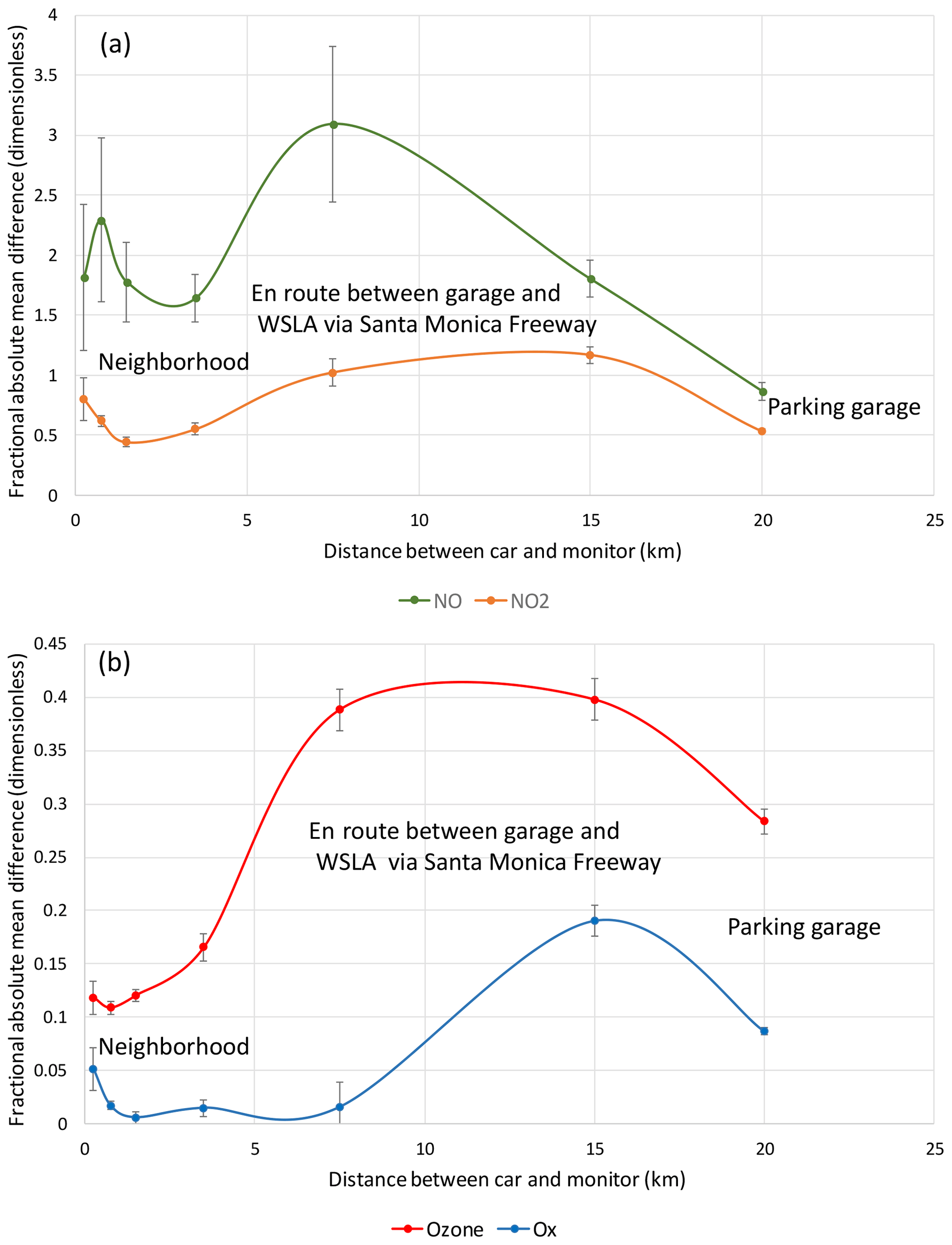
Figure 6 FAMD between mobile-platform monitoring and WSLA measurements versus distance between cars and WSLA on 4 d (13, 19, 26, and 29 September 2016) when the cars drove near WSLA. The first bin includes all distances less than 0.5 km; the minimum distance between cars and monitor was 158 m. Locations are indicated. One-sigma uncertainties of the FAMD were determined as described in the definition of FAMD in the text.

3.5 Differences between pollutant concentrations reported by vehicles operating in different neighborhoods

This section helps identify neighborhoods where pollutant concentrations are typically higher than they occur elsewhere, potentially indicating where long-term monitors could be located for characterizing higher pollution impacts. In such neighborhoods, air pollutant exposures may be higher than levels measured by regulatory monitors, since the latter are typically focused on community-scale air pollution.

3.5.1 San Francisco, May 2017

Measurements made by paired vehicles operating in different neighborhoods of San Francisco between 1 and 12 May 2017 are used to illustrate short-term (2-week) neighborhood-scale spatial variability. Example driving routes are shown as 1 s averages for 1 d in Fig. S10. The 1 s data were aggregated to 1 min averages, and the 1 min averages for all routes for 1–12 May are depicted in Fig. 7a. Different routes were taken on different days to obtain measurements in different neighborhoods in San Francisco. Since the averaging driving speeds between 1 and 12 May were 4.5 and 4.8 m s⁻¹ for Coltrane and Flora, respectively, the positions shown in Fig. 7a represent the midpoints of segments averaging 270–290 m.

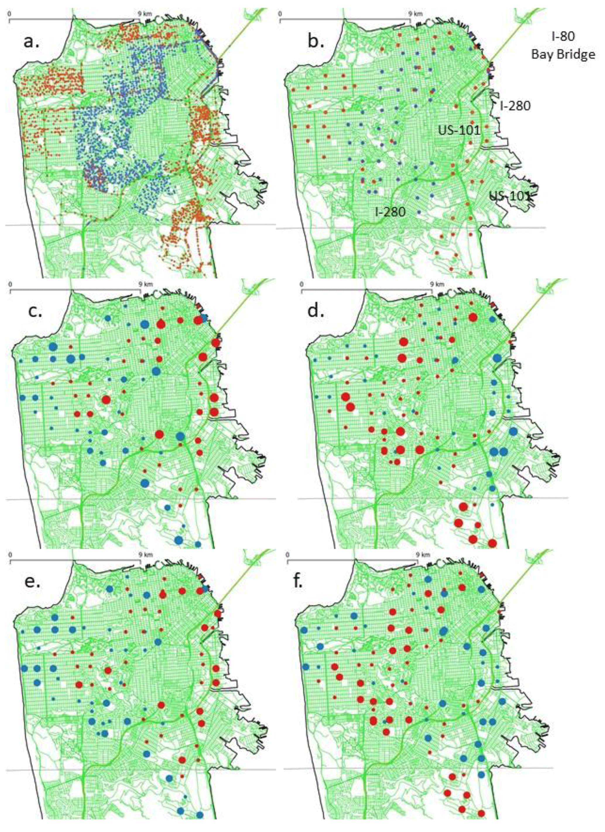
Figure 7 San Francisco sampling locations and results for 1–12 May 2017: (a) 1 min resolution locations (gold is Flora, lavender is Coltrane), (b) 1 km resolution locations (gold is Flora, lavender is Coltrane), (c) NO₂ intervehicle differences (red is positive, blue is negative; large symbol = < −4 or > 4 ppbv, medium $=-\mathrm{4}$ to −2 or 2 to 4 ppbv, small $=-\mathrm{2}$ to +2 ppbv), (d) O₃ intervehicle differences (same scale as NO₂), (e) NO₂ FMD (red is positive, blue is negative; large symbol = < −0.5 or > 0.5, small $=-\mathrm{0.5}$ to +0.5), (f) O₃ FMD (red is positive, blue is negative; large = < −0.05 or > 0.05, small $=-\mathrm{0.05}$ to +0.05). Maps generated with QGIS version 3.2.2 (https://qgis.org/en/site/, last access: 12 June 2020) open-source software licensed under the GNU General Public License (http://www.gnu.org.licenses, last access: 12 June 2020). California coastline shapefile obtained from the OpenStreetMap community (© OpenStreetMap contributors 2020, distributed under a Creative Commons BY-SA License; http://www.openstreetmap.org, last access: 12 June 2020) and MapCruzin (http://www.mapcruzin.com, last access: 12 June 2020), licensed under the Creative Commons Attribution ShareAlike 2.0 license. US highways and California county boundary shapefiles obtained from US Bureau of the Census TIGER/Line Shapefiles public data (https://www.census.gov/geographies/mapping-files/time-series/geo/tiger-line-file.html, last access: 12 June 2020).

One-minute averages were next averaged spatially to the nearest kilometer (based on conversion of latitude and longitude to Universal Transverse Mercator – UTM – coordinates) separately for each car (Fig. 7b), which is a spatial scale corresponding to about a 3 min average. However, the sampling times of the 1 km average concentrations varied by up to 6 h among locations, which confounds spatial with diurnal variability. Instead of analyzing 1 km average concentrations by vehicle, therefore, each 1 min average was paired with the corresponding 1 min average reported by the other vehicle, and synchronous concentration differences were determined. When these synchronous differences are averaged to 1 km resolution, they represent the average enhancement or deficit of a pollutant at a given 1 km location when compared to simultaneous measurements made elsewhere, i.e., the average excess or deficit relative to co-measured concentrations (Fig. 7c and d). This approach permits consideration of spatial variations in a manner that limits the confounding influence of diurnal variability and provides a better relative comparison of pollutant levels among neighborhoods.

One-kilometer averages consisting of fewer than 10 one-minute data points were excluded, yielding 97 of 236 possible spatial averages for NO₂ and 107 of 271 possible spatial averages for O₃. The decision to exclude 1 km averages consisting of fewer than 10 one-minute data points was based on the high standard errors of such averages (e.g., > 0.2 for the NO₂ FAMD when n < 10). The number of 1 min averages within each 1 km average ranged from 10 to 95 (i.e., 60–5700 one-second averages); for the 1 km average covering the parking garage, there were 1813 and 2520 one-minute O₃ and NO₂ averages, respectively.

For both NO₂ and O₃, most 1 km average concentration differences exceeding 2 ppbv (or < −2 ppbv) were statistically nonzero (i.e., the interval of the mean difference ±2 standard errors of the mean did not cover zero); most differences in the range between −2 and 2 ppbv were not statistically different from zero (Fig. 7c and d). These figures exclude the few larger differences that were not statistically different from zero (7 O₃ and 4 NO₂ averages), which may include atypical events. Both fractional differences and the signs (excess or deficiency) of the differences are of interest; therefore, the mean fractional differences are expressed as FMD rather than FAMD (Fig. 7e and f), since the sign of the difference is important. For NO₂, FMD values exceeding 0.5 (or < −0.5) were statistically different from zero; for O₃, FMD values exceeding 0.05 (or < −0.05) were statistically different from zero. The contrast in the detectability of nonzero fractional NO₂ and O₃ differences between vehicles (FMD) is pronounced but readily explained: the average intervehicle concentration differences were comparable for NO₂ and O₃ (Fig. 7c and d), but mean O₃ concentrations exceeded mean NO₂ concentrations (Table 8).

During 1–12 May, locations on the eastern side of San Francisco experienced higher NO₂ concentrations and lower O₃ concentrations than central and western locations (Fig. 7). This result is consistent with typically prevailing winds from the west to northwest and with high traffic volumes on major freeways, I-80 (Bay Bridge), I-280, and US 101, which are expected to yield higher emissions and ambient concentrations closer to areas with higher traffic volumes. Because fresh NO emissions initially reduce ambient O₃ concentrations, O₃ concentrations are typically lower where NO₂ concentrations are higher. The results of this limited analysis indicate that the measurement system can reveal differences among air pollutant levels occurring in different neighborhoods during short (i.e., days to weeks) time periods.

The San Francisco results reveal mean 1 km scale spatial differences in NO₂ and O₃ concentrations up to 117 % and 46 %, respectively, of mean values during the 2-week sampling period. The results obtained for 1 km averages can be further examined to demonstrate higher variability on smaller spatial scales. We compared the standard deviations of the 1 km mean intervehicle NO₂ differences to the corresponding 1 km mean NO₂ concentrations to characterize variability within 1 km spatial averages. These ratios (standard deviation of intervehicle difference / mean concentration) ranged from 0.5 to 3.0 (average =1.3). Within the 1 km averages, therefore, vehicle-to-vehicle NO₂ concentration differences varied by factors of 1–6 (twice the standard deviation of the mean differences) times the mean observed 1 km average concentrations.

Another indicator of spatial variability at finer resolution is the FMAD: as previously noted, the FMAD provides a measure of the variability in individual measurements because it averages absolute values of concentrations and is therefore relevant to understanding the comparability of high-resolution measurements. For the San Francisco data, the FMAD represents the variability in the 1 min time averages that comprise each 1 km spatial average. The average of the FMAD values across all 1 km spatial averages was 0.74, nearly twice as high as the average FAMD of 0.44.

Figure 8 San Joaquin Valley driving routes on 16 November 2016. The positions of each car at the beginning of each hour are marked. The drives began and ended at the parking garage in San Francisco. Locations of cities identified in the text are also shown. Map generated with QGIS version 3.2.2 (https://qgis.org/en/site/, last access: 12 June 2020) open-source software licensed under the GNU General Public License (http://www.gnu.org.licenses, last access: 12 June 2020). California coastline and state highway shapefiles obtained from the OpenStreetMap community (© OpenStreetMap contributors 2020, distributed under a Creative Commons BY-SA License; http://www.openstreetmap.org, last access: 12 June 2020) and MapCruzin (http://www.mapcruzin.com, last access: 12 June 2020), licensed under the Creative Commons Attribution ShareAlike 2.0 license. US highways and California county boundary shapefiles obtained from US Bureau of the Census TIGER/Line Shapefiles public data (https://www.census.gov/geographies/mapping-files/time-series/geo/tiger-line-file.html, last access: 12 June 2020).

3.5.2 San Joaquin Valley, November 2016

Over 10 months, driving routes in the northern San Joaquin Valley were located within the cities of Tracy (2017 population – 90 890), Stockton (320 554), Manteca (76 247), Merced (84 464), Modesto (215 080), and Turlock (72 879) (https://www.cacities.org/Resources-Documents/About-Us/Careers/2017-City-Population-Rank.aspx, last access: 2 December 2019) (Table 1). The initial drives occurred on 16–23 November 2016 (Fig. 8; see also examples of drives on other days in Figs. S11–S15). Because the destinations were located over 100 km from where the cars were parked overnight in the San Francisco parking garage, the cars drove longer distances and sampled more nonurban roads (both rural and high-traffic volume interstates) each day than they did in Los Angeles or San Francisco. The San Joaquin Valley car-to-car comparisons therefore provide insight into variations on larger spatial scales (e.g., 10–100 km), which are of interest for understanding enhancements of urban over nonurban pollutant concentrations as well as pollutant transport between cities or subregions.

Table 11 Dates, locations, and times when vehicle pairs sampled different areas within the northern San Joaquin Valley.

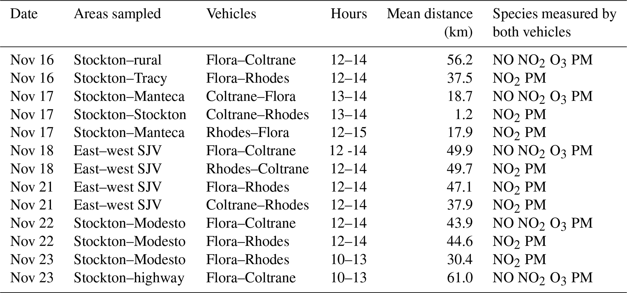
Table 12 Fractional mean differences (FMDs) when vehicle pairs sampled different areas within the northern San Joaquin Valley. Vehicles A and B correspond to the first and second areas sampled, respectively. Uncertainties are 1 standard error of the means. NA is not available; one car (Rhodes – R) measured only NO₂ and PM concentrations.

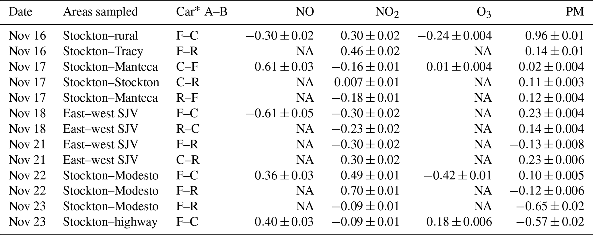
^* C is Coltrane, F is Flora, and R is Rhodes.

Between 16 and 23 November 2016, the cars drove on nonurban roads and on city streets in Stockton, Manteca, and Modesto, providing information on pollutant concentrations in Stockton relative to other portions of the northern San Joaquin Valley and in the eastern half of the San Joaquin Valley compared with the western side (Table 11; Figs. 7 and S11–S15). For each geographical pairing, pollutant enhancements varied by pollutant and date (Table 12; see Tables S1–S4 for detailed tabulations). For example, relative to sampling in both a rural area and near I-205 in Tracy, Stockton exhibited enhancements of NO₂ concentrations and PM_0.3−0.5 counts on November 16 along with deficits of NO and O₃. Since mean NO_x (NO+NO₂) concentrations in Stockton (31.3 ppbv) did not differ from the rural route (31.8 ppbv) (Tables S1, S2), the Stockton–rural differences in NO and NO₂ concentrations may have been related to atmospheric chemical reactions and air mass aging. On November 23, the Stockton–highway comparison exhibited the opposite pattern to November 16: deficits of NO₂ concentrations and PM_0.3–0.5 c L⁻¹ along with enhancements of NO and O₃ (Table 12) compared to routes in Modesto (within 1 km of Highway 99) and along Highway 99 (Modesto to Merced), Highway 140 (Highway 99 to I-5), and I-5 (Figs. S15). High traffic volumes (∼50 000–150 000 vehicles per day, annual average peak volumes) are typical of Highway 99 (https://dot.ca.gov/programs/traffic-operations/census/traffic-volumes, last access: 15 April 2020), so the results on 23 November indicate higher pollutant concentrations on and near major highways than on city streets in Stockton and in Modesto (Tables 12, S2–S5).

The spatial analyses do not show consistent enhancements of pollutant concentrations in northern San Joaquin Valley cities over concentrations occurring in surrounding areas. This result suggests a complex situation in which pollutant levels in the study cities depend on both local emissions and intra-regional pollutant transport. Similarly, the relationships between measured concentrations and intervehicle distance in the San Joaquin Valley depend upon the locations of the vehicles (Fig. S16). Results for 16 November are shown for multiple species in Fig. S17. NO₂ and particle numbers exhibited FAMDs exceeding 0.2 over most intervehicle distances. The largest FAMDs for NO₂ and particle numbers were associated with contrasts between locations within the San Joaquin Valley and locations along an upwind boundary; these contrasts appear as intervehicle distances of 50–80 km, corresponding to times when Coltrane traversed the highway between San Jose (hour 11) and Crows Landing (near hour 14 at I-5 in the San Joaquin Valley) while Flora was sampling city streets in Stockton (Fig. 7). Paired O₃ values were similar (FAMD < 0.2 up to intervehicle distances of 50 km), illustrating the regional character of O₃ in much of the northern San Joaquin Valley. The smaller FAMDs at 25 and 45 km intervehicle distances occurred when both vehicles were sampling freeway locations in the urban San Francisco Bay Area (Fig. S17). The larger FAMDs at intervehicle distances of 15 km occurred when the cars traversed I-580 between Manteca and Hayward (near Castro Valley Freeway; Fig. 8) on their return trip in the afternoon, and the vehicles experienced differences in traffic levels due to their positions in urbanized versus nonurban portions of I-580 (hour 15; Figs. 8, S17).

3.6 Spatial representation of measurements from regulatory monitors

Comparisons of mobile-platform concentrations to concentrations recorded by the downtown Los Angeles stationary monitor (CELA) showed that the FAMD for NO largely exceeded 1 (100 %); most NO₂ and all O₃ FAMDs were less than 0.2 (20 %) at car–monitor distances ranging from 0.5 to 4 km. The results indicate that the US EPA classification of the downtown Los Angeles location as a neighborhood-scale site (0.5–4 km zone of representation; Table 3) is appropriate for NO₂ and O₃. Comparisons of mobile monitors to data from the western Los Angeles monitor (WSLA) showed that the mobile platforms recorded much higher concentrations of NO and NO₂ than the monitor at vehicle-to-monitor distances ranging from < 0.5 to 5 km; for NO and NO₂, the FAMD exceeded 1.5 (150 %) and 0.6 (60 %), respectively. The results support the US EPA classification of WSLA as a middle-scale site (100 m to 0.5 km zone of representation; Table 3). The methods used for evaluating the spatial representativeness of CELA and WSLA are readily applied to other locations.

3.7 Effectiveness of the driving routes for addressing study questions

Driving routes followed in this study were intended to address various research questions focused on evaluating mobile-platform performance and spatial scales of representativeness (per previous subsections in “Results and discussion”). Different routes were deployed for different questions. The routes utilized in the comparisons with stationary regulatory monitors in Los Angeles provided effective coverage of neighborhoods located 100 m to 4 km from two stationary monitors. The results supported the EPA classifications of those monitors.

The sampling conducted in San Francisco was intended to delineate spatial variations in pollutant concentrations across the city. Sampling during a single 2-week period, which covered a subset of a compact urban environment, clearly revealed 300 m–1 km spatial differences in pollution concentrations but varied by pollutant. In contrast, sampling was conducted over a much larger area in the northern San Joaquin Valley, and the results were difficult to interpret from a limited (2-week) set of measurements because the spatial domains sampled were different on different days. For example, contrasts between an urban area (Stockton) and areas surrounding Stockton were expected to yield information on the urban pollution enhancement in Stockton. However, three different types of environments were sampled in conjunction with the initial 2 weeks of Stockton measurements: (1) nearby cities (e.g., Manteca, Tracy, and Modesto, located 19 to 45 km from Stockton), (2) a major freeway (Highway 99, mean distance 61 km from Stockton), and (3) a rural area (56 km from Stockton). Establishing quantitative contrasts for each of these comparisons likely requires at least 2 weeks of data for each type of comparison (e.g., Stockton vs rural). Such comparisons could be explored using the full San Joaquin Valley data set.

4 Conclusions

The Aclima, Inc., mobile measurement and data acquisition platform, which equips Google Street View cars with research-grade instruments to measure air quality at high spatial resolution, is an effective approach to obtaining improved understanding of spatial variations in air pollutant concentrations. Data provided by the system will be highly useful for evaluating air quality management policies intended to reduce human air pollutant exposure, acute and chronic health impacts, and premature mortality. Audit results demonstrate that reference instruments in stationary vehicles are capable of reliably measuring NO, NO₂, O₃, and PN, with bias and precision ranging from < 5 % to < 25 % at 1 s time resolution.

During experiments conducted in Los Angeles, San Francisco, and the San Joaquin Valley, California, collocated parked and moving mobile platforms replicated mean NO, NO₂, and O₃ concentrations with mean differences in 1 s measurements ranging from 0.2 to 5.6 ppbv; mean differences in PN_0.3–0.5 varied from 500 to 21 000 c L⁻¹. On a relative basis, the mean differences between replicate mobile platforms ranged from 1 % to 37 % of the mean NO, NO₂, and O₃ concentrations and 2 % to 32 % of PN, with higher mean differences observed in the larger particle size ranges (which also had few numbers of particles). The majority (21 of 26) of comparisons of collocated mobile platforms exhibited differences < 20 % of the mean concentrations, thereby suggesting that differences exceeding 20 % obtained by vehicles operating simultaneously in different neighborhoods represented measurable spatial variation.

Paired time-synchronous mobile measurements were used to characterize the spatial scales of concentration variations when vehicles were separated by < 1 to 10 km. Measurements made in Los Angeles during August 2016 exhibited intervehicle FAMDs that ranged from 2 % at 0.125 km to 14 %–44 % at 4.5–5.5 km (mean 12 %) for NO₂ and from 0.6 % at 0.125 km to 0 %–7 % at 4.5–5.5 km (mean 2 %) for O₃. The standard deviations of bin averages indicated that finer-scale (e.g., 100–300 m, 1 min averages) intervehicle variations were larger, indicating variability by up to a factor of 2 for NO₂ and a factor of 6 for NO (2 standard deviations) within the binned intervehicle averages.

For NO and PN_0.3–0.5, bin-average mean differences exceeded 20 % for the same driving routes, indicating measured spatial variability exceeding the uncertainties in measurement methods when employing the mobile platforms. For NO, the standard deviations of bin averages ranged from 1.2 to 4.0 (average $=\mathrm{2}.$8), indicating that vehicle-to-vehicle NO concentration differences varied by up to a factor of 6 (2 standard deviations) within the binned intervehicle averages.

A data analysis approach was developed to characterize spatial variations in a manner that limits the confounding influence of diurnal variability. The approach involved examining synchronous differences between 1 min measurements made by two mobile platforms, which were then averaged to 1 km resolution. The approach was illustrated using data from San Francisco, revealing mean 1 km scale spatial differences in NO₂ and O₃ concentrations up to 117 % and 46 %, respectively, of mean values during a 2-week sampling period. Within the 1 km averages, vehicle-to-vehicle NO₂ concentration differences varied by factors of 1–6 times the mean observed 1 km average concentrations, implying higher variability at spatial scales < 1 km (i.e., among 1 min averages, corresponding to ∼300 m distances). Locations on the eastern side of San Francisco experienced higher NO₂ concentrations and lower O₃ concentrations than central and western locations, likely due to differences in traffic density and to meteorological factors, with prevailing winds from the west or northwest.

The mobile data were also used to provide insight into the spatial representativeness of measurements made at stationary monitoring locations. Comparisons of mobile measurements to data from two stationary monitors in Los Angeles indicate that the US EPA classifications of the monitors as representative of neighborhood-scale (0.5–4 km) or middle-scale (100 m–0.5 km) pollutant concentrations are appropriate. The methods used for evaluating the spatial representativeness of the two monitors are readily applied to other locations.