the Creative Commons Attribution 4.0 License.
the Creative Commons Attribution 4.0 License.
 | 16 Jul 2020
Confronting the boundary layer data gap: evaluating new and existing methodologies of probing the lower atmosphere
Brian R. Greene
Petra M. Klein
Matthew Carney
Phillip B. Chilson
It is widely accepted that the atmospheric boundary layer is drastically under-sampled in the vertical dimension. In recent years, the commercial availability of ground-based remote sensors combined with the widespread use of small, weather-sensing uncrewed aerial systems (WxUAS) has opened up many opportunities to fill this measurement gap. In July 2018, the University of Oklahoma (OU) deployed a state-of-the-art WxUAS, dubbed the CopterSonde, and the Collaborative Lower Atmospheric Mobile Profiling System (CLAMPS) in the San Luis Valley in south-central Colorado. Additionally, these systems were deployed to the Kessler Atmospheric and Ecological Field Station (KAEFS) in October 2018. The colocation of these various systems provided ample opportunity to compare and contrast kinematic and thermodynamic observations from different methodologies of boundary layer profiling, namely WxUAS, remote sensing, and the traditional in situ radiosonde. In this study, temperature, dew point temperature, wind speed, and wind direction from these platforms are compared statistically with data from the two campaigns. Moreover, we present select instances from the dataset to highlight differences between the measurement techniques. This analysis highlights strengths and weaknesses of planetary boundary layer profiling and helps lay the groundwork for developing highly adaptable systems that integrate remote and in situ profiling techniques.
- Article
(14780 KB) - Full-text XML
- BibTeX
- EndNote


It has been a decade since the National Research Council (2009) published their report detailing the need for a mesoscale observation network that extends vertically beyond the Earth's surface. It was concluded that vertical profiles in the boundary layer are inadequately measured in both space and time. At the time, the only operational method of resolving the thermodynamic and kinematic properties of the boundary layer was with radiosondes launched twice daily by weather services around the world, which has been conducted since the 1930s. However, radiosondes spend only a limited amount of time in the boundary layer every day. Due to the importance of the boundary layer characteristics to areas like air quality forecasts (World Health Organization, 2016; Park et al., 2016; Bessagnet et al., 2019), convective initiation (e.g., Nowotarski et al., 2011; Markowski and Bryan, 2016; Markowski, 2016; Koch et al., 2018), and wind energy forecasting (e.g., Zhou and Chow, 2012), more observations are needed to fill the spatial and temporal data gap that exists to date. The recent Decadal Survey by the National Academy of Sciences (National Academies of Sciences and Medicine, 2018) further reinforces this by identifying boundary layer processes as key to improving weather and climate models. To fill this data gap, two different paradigms have been suggested: ground-based remote sensing and uncrewed aircraft systems (UAS, also referred to as remotely piloted aircraft systems, RPAS). Both paradigms have particular strengths and weaknesses that need to be characterized before a system can be proposed for widespread adaptation.
A workshop was conducted shortly after the NRC report was published that identified several possible ground-based remote sensing platforms that could augment current upper-air and satellite observations (Hoff and Hardesty, 2012). Attendees generally agreed that instruments needed to have accuracy within 1 ∘C for temperature and 1 g kg−1 for moisture while having a vertical resolution of 30–100 m. Additionally, the NRC report recommended a temporal resolution ranging from 15 min to 3 h, depending on the phenomena (National Research Council, 2009). At the time, three platforms largely met these requirements: microwave radiometers (MWR), atmospheric emitted radiance interferometers (AERI), and water vapor differential absorption lidars (WV-DIAL). Of these, the MWR and AERI stood out due to their ability to retrieve both temperature and moisture profiles, along with several other variables. Both instruments measure downwelling radiation emitted by the atmosphere. The measured bands encompass spectral regions where gases have absorption features. These observations can be fed into multiple types of retrievals to obtain thermodynamic profiles of the atmosphere. While the WV-DIAL can provide higher-resolution measurements, at the time of writing there are still no commercially available WV-DIAL systems.
However, these remote sensing systems are expensive and multiple instruments are required to achieve both thermodynamic and kinematic profiles of the boundary layer. Recent workshops have identified UAS as a potential way to get high-resolution thermodynamic and kinematic profiles of the boundary layer. For example, the National Center for Atmospheric Research Earth Observing Laboratory held a workshop focused on the use of UAS in atmospheric research (Vömel et al., 2018). They identified various areas in which improvements are needed for weather-sensing UAS to be put to widespread use, with one of the most important being the need for a standard sensor packages for the various types of systems.
Due to regulatory issues related to integration of UAS into the National Airspace System (NAS), UAS are currently less developed and less utilized than remote sensors (Hoff and Hardesty, 2012; Koch et al., 2018), though the use of UAS is expected to continue to increase as further advances in GPS and communication allow for safer operation in public airspace (Geerts et al., 2018). Additionally, as commercial applications of UAS continue to emerge (e.g., remote package deliveries, infrastructure inspection, and agricultural monitoring) and safety cases are developed, the Federal Aviation Administration (FAA) will have to plan and account for UAS in the NAS.
Traditionally, observations of the atmosphere using weather-sensing UAS (WxUAS) utilized fixed-wing aircraft (e.g., Reuder et al., 2009; Chilson et al., 2009; Houston et al., 2012; Reuder et al., 2012; Bonin et al., 2012; Balsley et al., 2013; Lawrence and Balsley, 2013; Lothon et al., 2014; Wildmann et al., 2014, 2015; Båserud et al., 2016; de Boer et al., 2016). Using fixed-wing WxUAS allowed researchers to leverage major technological advances from decades of measurement research from piloted aircraft (e.g., Saïd et al., 2005; Gioli et al., 2006; van den Kroonenberg et al., 2012). Additionally, fixed-wing WxUAS are capable of flight times of an hour or more, allowing researchers to cover a large spatial range.
However, the recent commercial boom of UAS has made rotary-wing UAS (rwUAS) easily accessible to the public. Researchers are now turning to rwUAS because they are more versatile, readily available, and relatively easy to operate. A common application of rwUAS in atmospheric science is collecting thermodynamic and kinematic variables as a function of altitude, similar to the traditional radiosonde. Forecasters and researchers can use the same conceptual framework as radiosondes to analyze and interpret data from rwUAS profiles. In a sense, the framework is even more applicable since rwUAS can remain over the same geographical location during observations while radiosondes drift many kilometers downwind.
Using rwUAS poses new challenges that must be overcome before they can be considered a viable platform for atmospheric observation. For example, rwUAS modify the environment surrounding them, so measuring even simple variables like temperature can be difficult. Careful considerations must be made to ensure the true environmental temperature is being measured, as opposed to the modified rwUAS environment. Additionally, proper aspiration of the sensors and shielding from solar radiation is vital to accurate measurements (Tanner et al., 1996; Hubbard et al., 2004; Greene et al., 2018, 2019).
In this study, a comparison is made between results from a rotary-wing WxUAS and different ground-based remote sensors against data from the historical standard: the radiosonde. Observations of the temperature, dew point temperature, wind speed, and wind direction of the lower atmosphere were collected during two field campaigns under different environmental conditions with the instruments operating at the same time and from the same location. This provided an opportunity to both compare results from various instruments and consider the strengths and weaknesses of the methodologies considered. Though comparisons between radiosondes and the ground-based remote sensors used in these campaigns are not novel (Pearson et al., 2009; Turner and Löhnert, 2014; Blumberg et al., 2015; Päschke et al., 2015; Koch et al., 2018; Turner and Blumberg, 2018), it is important to perform these comparisons for this study to assist in identifying and characterizing the uncertainty in all the systems. As mentioned before, previous studies have worked to mitigate the effect of the UAS on the thermodynamic measurements, which decouples the UAS technique from the sensor themselves (Greene et al., 2018, 2019). However, these studies were performed in relatively idealized conditions. The purpose of this study is to verify that these results hold in a more “operational” mode. In addition to the comparisons, synergies between the various systems are identified and discussed. The following sections contain more information about the instrument systems and the field campaigns, an analysis of the results, and a summary of the findings.
For this study, the three profiling platforms that are compared consist of the Collaborative Lower Atmospheric Mobile Profiling System (CLAMPS), the CopterSonde, and radiosondes. Each platform is described in detail below.
2.1 CLAMPS
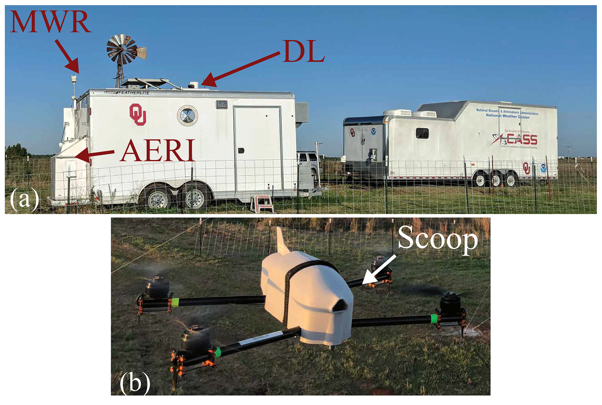
CLAMPS consists of an AERI (Knuteson et al., 2004a, b), a Version 4 Humidity and Temperature Profiling MWR (HATPRO; Rose et al., 2005), and the Halo Photonics Streamline scanning Doppler lidar (DL; Pearson et al., 2009) in a modified off-the-shelf trailer (Fig. 1a). The CLAMPS facility also has the ability to launch radiosondes as there is storage for multiple helium tanks and an antenna mounted on top of the trailer (Wagner et al., 2019). The DL scan strategy consisted of an 18-point velocity azimuth display at 70∘ elevation (VAD; Browning and Wexler, 1968; Päschke et al., 2015) and a 6-point VAD at 45∘ elevation every 5 min to gather profiles of wind speed and direction. For the following analysis, only the 18-point VAD scan is used. When the DL was not performing these VAD scans, it was staring vertically to collect vertical velocity statistics.
Thermodynamic variables were collected using the AERI and MWR in a joint retrieval. The AERI Optimal Estimation (AERIoe; Turner and Löhnert, 2014; Turner and Blumberg, 2018) is a physical retrieval that retrieves temperature and water vapor profiles using an iterative optimal estimation technique (Rodgers, 2000). For the retrievals in this study, surface data from a Vaisala WXT-530 weather station mounted 3 m above ground level (a.g.l.) on the back of CLAMPS was used to constrain the temperature and moisture at the surface. Additionally, colocated radiosondes were used to constrain the upper atmosphere above 3 km a.g.l. since nearly all the information contained in the AERI measurement is contained in the lowest 2 km of the atmosphere (Turner and Löhnert, 2014). The backscatter from the DL vertical stare was used to detect cloud base in the retrieval.
2.2 CopterSonde 2.5
The WxUAS used by the University of Oklahoma (OU) is the CopterSonde v2.5 (hereafter, just CopterSonde). The CopterSonde is the second iteration of the rwUAS that is described in detail in Greene et al. (2018). The original CopterSonde was built and deployed by the Center for Autonomous Sensing and Sampling (CASS) at OU for the Environmental Profiling and Initiation of Convection (EPIC; Koch et al., 2018) field campaign. CASS originally planned to use an off-the-shelf rwUAS, but it was determined that an airframe was not available to account for the specific needs of environmental sampling and instead opted to build a custom WxUAS. The original CopterSonde was successfully built and deployed for the EPIC campaign but found mixed success in providing accurate and reliable atmospheric thermodynamic data (Koch et al., 2018).
Deployment of the original CopterSonde provided many valuable lessons on how to improve upon its design and mode of operation. This led to the development of the CopterSonde for deployment in the 2018 Innovative Strategies for Observations in the Arctic Atmospheric Boundary Layer (ISOBAR) campaign (Kral et al., 2018). The CopterSonde is a quad-copter designed specifically for thermodynamic and kinematic profiling. Instead of temperature and humidity sensors being “passengers” on the CopterSonde, they are directly integrated into the nose of the craft utilizing a custom 3D printed shell and are read by custom autopilot code. Additionally, the CopterSonde is programmed to always turn into the wind. This combined with radiation shielding and a ducted fan to aspirate the sensors increases the precision of the measurements from the platform, which minimizes the effect of the platform itself on the sensors (Greene et al., 2019). More details of the development of the CopterSonde can be found in Segales et al. (2020).
Data from the CopterSonde are processed to a 3 m vertical resolution starting from 6 m a.g.l. in order to not contaminate the profile with effects induced by the ground. The temperature measurements were made using three iMet-XF glass bead thermistors while the relative humidity measurements were made using three Innovative Sensor Technology HYT 271 relative humidity sensors. Three sensors were used for redundancy; if one sensor goes bad, the other two can be used to automatically identify the bad sensor. If only two sensors were used and a sensor malfunctioned, it would be difficult to determine the faulty sensor automatically. Wind speed and direction are calculated by using a methodology based on Neumann and Bartholmai (2015), which uses the tilt of the airframe to estimate the velocity. This is done in real time so that custom autopilot software can always direct the nose of the CopterSonde into the wind, which improves thermodynamic and kinematic measurements (Greene et al., 2019). Herein, the thermodynamic package and ducted fan are referred to as the “scoop”.
The sensors in the CopterSonde scoop were characterized in the Oklahoma Climatological Survey calibration laboratory. The entire scoop was placed inside of a controlled calibration chamber and aspirated using the ducted fan to account for any heat that may come off of the fan. The scoop was calibrated for 1 h periods at multiple chamber reference temperatures and humidities. Data from each sensor in the scoop were compared to a calibrated thermistor and a chilled-mirror hygrometer and any sensor bias was corrected. CopterSonde data used in this analysis have had these correction curves applied.
2.3 Radiosondes
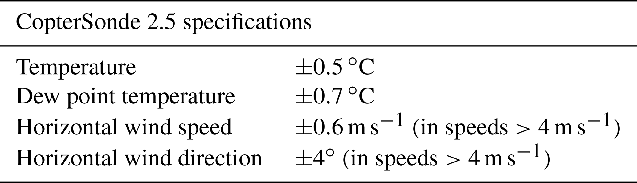
The Vaisala RS92-SGP was the radiosonde used for this study. The data used in the comparisons was processed using the Vaisala ground station software. The targeted ascent rate was 5 m s−1 with the radiosonde reporting to the ground station every second. The files used for the analysis were post-processed to 2 s resolution. The Vaisala RS92-SGP has a temperature uncertainty of 0.5 ∘C, relative humidity uncertainty of 5 %, wind speed uncertainty of 0.15 m s−1 (at wind speeds >3 m s−1), and wind direction uncertainty of 2∘ according to the Vaisala specifications.
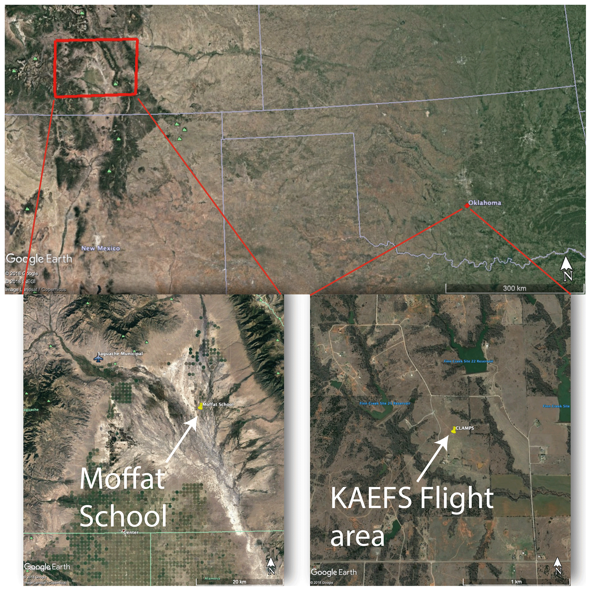
Figure 2Location and domain size for the LAPSE-RATE (a) and Flux Capacitor (b) campaigns. During LAPSE-RATE, OU was deployed at both the Saguache Municipal Airport and the Moffat School; however, only the Moffat data will be analyzed in this study (satellite images © 2018 Google).
The CopterSonde and CLAMPS were colocated for two field experiments in 2018: Lower Atmospheric Process Studies at Elevation – a Remotely piloted Aircraft Team Experiment (LAPSE-RATE) and Flux Capacitor. These experiments together provide a wide range of conditions under which the CopterSonde and CLAMPS were evaluated. The experiments are described below.
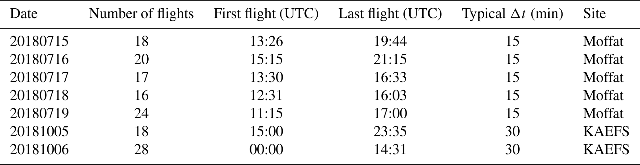
Table 1Summary of flights at the Moffat School and KAEFS. In total, 141 flights were used in the comparison. The fifth column lists the typical cadence of flights, typical Δt, which corresponds to the typical amount of time between flights.
3.1 LAPSE-RATE
In July 2018, OU deployed the CopterSonde and CLAMPS in the San Luis Valley in south-central Colorado (Fig. 2a) as part of Lower Atmospheric Process Studies at Elevation – a Remotely piloted Aircraft Team Experiment (LAPSE-RATE, de Boer et al., 2020). LAPSE-RATE was a week-long experiment with the goal of dispersing UAS throughout the valley to study various atmospheric phenomena, including convective initiation, cold air drainage, and morning transitions. Broader goals were to further evaluate and advance UAS that have been developed for atmospheric sensing in recent years. LAPSE-RATE was organized in connection with the annual meeting of the International Society for Atmospheric Research using Remotely piloted Aircraft (ISARRA). Over 100 participants from 16 institutions took part in the campaign. The flight teams logged almost 1300 individual flights, with CASS contributing nearly 200 of those flights. During the week, one of the largest UAS intercomparison and calibration efforts to date also took place, highlighting some of the thermodynamic and kinematic sampling biases inherent to different varieties of aircraft (Barbieri et al., 2019).
The San Luis valley provided a unique opportunity to study flow in complex terrain, due to it being surrounded by mountains to the east and west. The valley floor is primarily flat shrubland and irrigated agricultural fields (Fig. 2a). The mountains create complex thermal flows while the irrigated fields on the western half of the valley, in contrast with the shrubland on the eastern half, create complex near-surface moisture gradients.
OU primarily operated at two sites during the campaign, the Moffat Consolidated School in the center of the valley and the Saguache Municipal Airport, which was 25 km to the northwest of the Moffat School. For one mission, the OU team at Saguache Municipal Airport relocated 10 km to the southeast to capture drainage flow from the mountains. CLAMPS was located at the Moffat School and CopterSondes were flown at both sites. Based on permission from the FAA, flights were conducted from the surface to 910 m a.g.l. along a vertical trajectory. Three different CopterSondes were flown during the LAPSE-RATE campaign. Two of the CopterSondes were flown solely at the Moffat School. The third was flown at Saguache and the drainage flow site mentioned above. Since all three scoops were characterized in the calibration chamber, there should be minimal difference in the measurements from each platform given that they are otherwise identical. Additionally, the CopterSonde was validated against a 15 m mobile mast during the LAPSE-RATE campaign (Barbieri et al., 2019).
3.2 Flux Capacitor
The Flux Capacitor campaign was an internally funded experiment organized by various groups at OU. One of the main goals was to evaluate the performance of the CopterSonde over a full diurnal cycle in support of the 3D Mesonet concept (Chilson et al., 2019). The campaign took place at the Kessler Atmospheric and Ecological Field Station (KAEFS) in October 2018. KAEFS is located 28 km southwest of the OU Norman campus and has been the main test site for the CopterSonde. In addition, KAEFS facilitates instrumentation from multiple research groups at OU, including the Washington site of the Oklahoma Mesonet.
For Flux Capacitor, CLAMPS was again colocated with the launch site for the CopterSonde (Fig. 2b), allowing comparisons between the systems. CopterSonde flights were conducted on a 30 min interval up to a max altitude of 1200 m a.g.l. In total, 46 flights were conducted over a 24 h period (Table 1). Two flights were missed due to mechanical issues with the CopterSonde, which have since been addressed.
Details of the number and times of flights used in this analysis (from both campaigns) are shown in Table 1.
To evaluate the different instruments, a detailed statistical comparison of each system relative to the others is shown in Sect. 4.1 and a couple of case studies are shown in Sect. 4.2. The statistical comparison provides an overall picture of how well the systems perform relative to one another while the case studies identify specific issues that can appear in data from each system. Herein, statistical comparisons are calculated using the open-source python packages NumPy (van der Walt et al., 2011), SciPy (Virtanen et al., 2019), and scikit-learn (Pedregosa et al., 2011), and figures are visualized using Matplotlib (Hunter, 2007).
4.1 Statistical comparison of systems
It is important to characterize differences statistically to draw conclusions about system performance relative to each other. For each of the system combinations (CLAMPS–Copter, CLAMPS–Radiosonde, Copter–Radiosonde), data from all heights and from both campaigns are compared to one another. A large number of data points are needed to draw any conclusions since the measurements from each platform are based on different assumptions and affected by different sources of error. While all three profiling methods are most often interpreted as a perfect vertical profile, this is obviously not true. For example, the VAD scan assumes that the wind field is horizontally homogeneous and stationary in order to retrieve the horizontal wind vector. This means the DL observations are averaged spatially both in terms of radial bins and the plan position indicator (PPI) scan required to calculate the VAD. Additionally, radiosondes drift and can often be collecting in situ measurements far from the launch point. So while comparing the systems one-to-one may not be ideal, at this point it is the best approach available to us.

Figure 3Example profile of temperature (red) and dew point temperature (blue) from each observation platform (a) and a time height cross section of vertical velocity measured from the CLAMPS DL from the same time period (b). The grey areas in (b) indicate the DL was not in vertical stare mode and was performing PPI scans.
Due to these limitations, any spread in the data presented from the following analyses contains three components: one component from instrument imprecision, one from the inability of the instruments to measure the same point at precisely the same time, and one component that arises from the differences in measurement technique. The goal of this study was to examine the spread that arises from the measurement technique itself.
Therefore, in order to eliminate any differences due to changing atmospheric conditions, data points with a difference that lies outside the 2σ envelope are considered outliers and were removed from the analysis. As a result, most of the comparisons had under 10 % of the points removed. However, the kinematic comparison between the radiosonde and the DL had the largest percentage of points removed at 33 %. This was due to a combination of fewer overall points and the VAD technique and radiosondes struggling to capture the very low wind speeds observed during the daytime hours of LAPSE-RATE. In general, approximately 15 % of profiles had at least one outlier. Of these 15 %, the median number of outliers per profile was two. These outliers followed no apparent pattern and would not contribute to any observed bias.
The outliers from the thermodynamic comparisons exhibited a different pattern. While fewer profiles overall contained outliers, there tended to be more outliers within these profiles. After analyzing these cases in depth, it was concluded that most of the outliers were likely due to changing atmospheric conditions between measurement times. For example, in the case of the CopterSonde and radiosonde comparison, outliers were found when the CopterSonde and radiosonde traversed temperature and moisture gradients at slightly different times during the morning boundary layer transition. The profile that contained the most outliers, along with some supplementary data from the CLAMPS DL, is shown in Fig. 3.
During this comparison, the radiosonde was launched promptly at 16:00 UTC on 17 July 2018. Due to the very low winds, the radiosonde did not clear the flight area immediately and the CopterSonde flight had to be delayed by 20 min. When the CopterSonde launched at 16:02 UTC, the radiosonde had already traversed a small inversion at 450 m a.g.l. The CopterSonde also observed this inversion, though it was at 620 m a.g.l. The outliers from this profile were in the layer between 450 and 620 m where the inversion changed height. The likely cause of this rapid change in inversion height was an updraft that formed between 16:00 and 16:06 UTC (Fig. 3b). During this time period, it was noted that a cloud formed while the CopterSonde was ascending. Referencing classical parcel theory, the updraft lifted and cooled the parcel to the lifted condensation level where latent heat release from condensation warmed the environment and modified the lapse rate. This same pattern was observed in multiple thermodynamic profiles that contained outliers and would add bias to the comparisons that originates from different error sources than those being studied here.
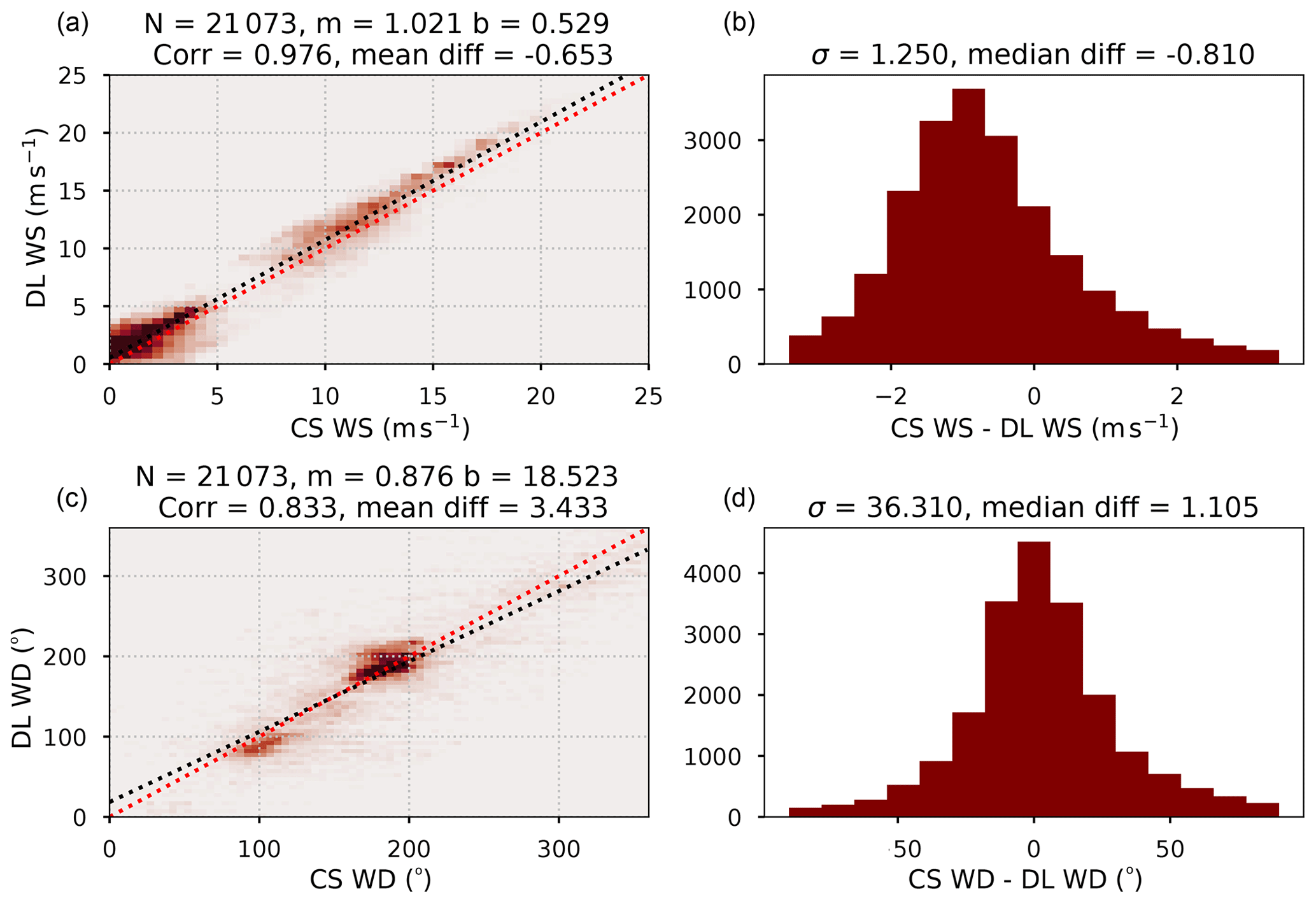
Figure 4Two-dimensional histograms of DL-measured wind speed vs. CopterSonde-measured wind speed (a) and DL-measured wind direction vs. CopterSonde-measured wind direction (c). The 2D histograms are binned to 0.5 m s−1 for wind speed and 5∘ for wind direction. The histograms on the right show the difference in wind speed (b) and wind direction (d). The dotted red line is the one-to-one line and the black line is the least-squares regression. The slope (m) and intercept (b) are shown in the title. Various other statistics are also shown in the titles. N corresponds to the number of points, Corr is the Pearson correlation, mean diff is the mean difference between the CopterSonde and the DL, σ is the standard deviation of the differences, and median diff is the median difference between the CopterSonde and the DL.
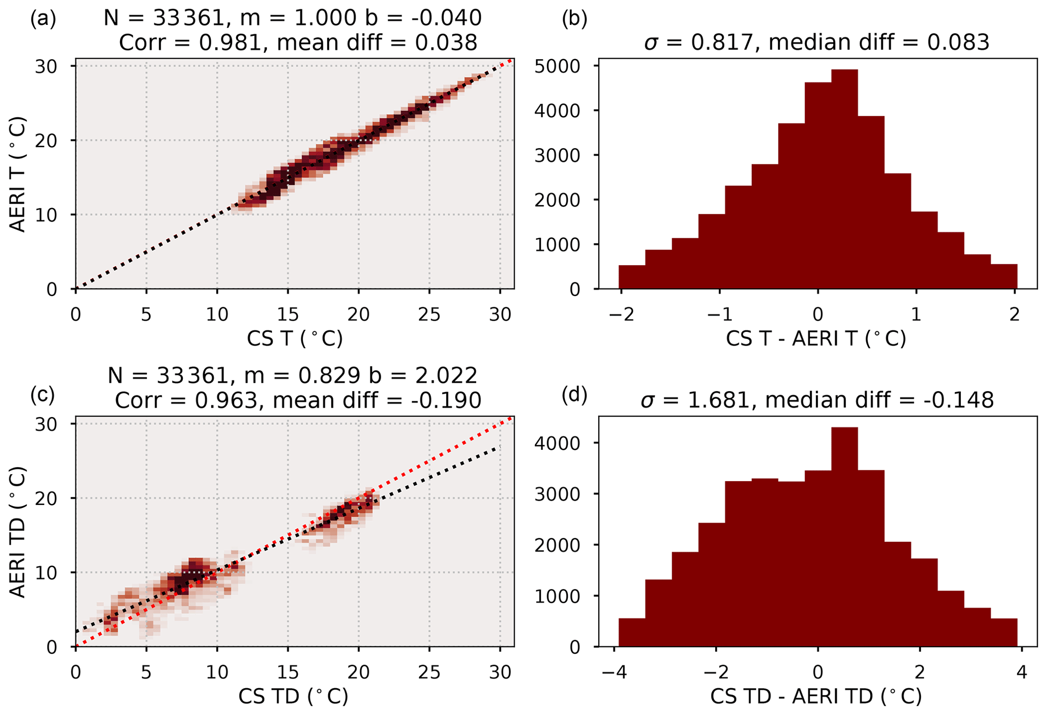
Figure 5Similar to Fig. 4 but for the temperature (a, b) and dew point temperature (c, d). The 2D histograms of temperature and dew point temperature are binned by 0.5 ∘C.
4.1.1 CLAMPS vs. CopterSonde
Kinematic and thermodynamic data from CLAMPS and the CopterSonde are presented in Figs. 4 and 5, respectively. The wind speed and direction from the CopterSonde and the 12-point VAD performed by CLAMPS compare remarkably well. In general, wind speeds less than 5 m s−1 are from LAPSE-RATE while the higher wind speeds are associated with the low-level jet observed during Flux Capacitor. The Pearson correlations (hereafter, just “correlation”) between wind speed and wind direction are 0.976 and 0.83, respectively. There is some disagreement in wind speed between the VAD and the CopterSonde, especially at higher wind speeds. This is discussed more in the next section.
The observed wind directions are largely bi-modal (Fig. 4c), with one group of observations around 90∘ and one group around 180∘. The group around 180∘ largely consists of observations from the Flux Capacitor dataset (southerly low-level jet), while the group around 90∘ is largely from LAPSE-RATE (easterly katabatic flows from mountains). Additionally, there are points scattered elsewhere that are also largely from LAPSE-RATE.
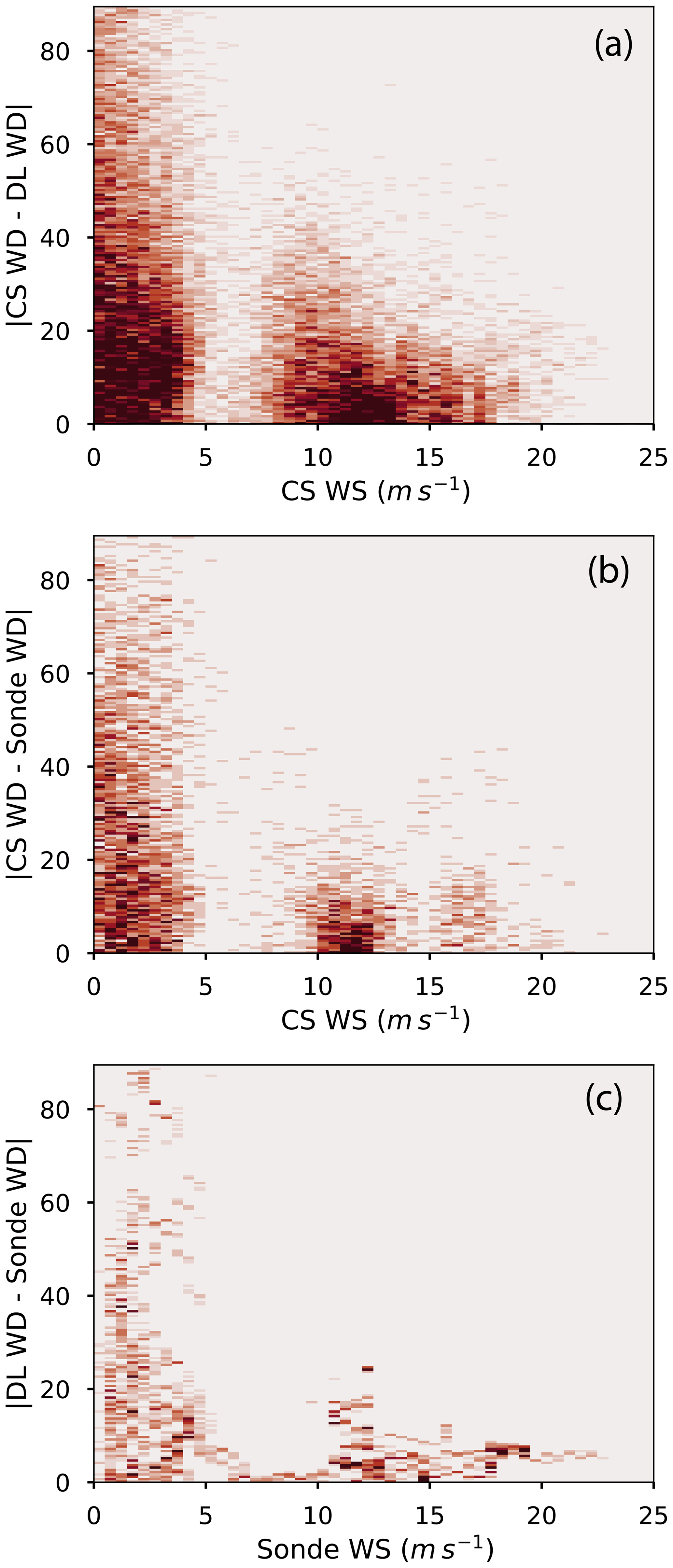
Figure 6Two-dimensional histograms of absolute wind direction difference vs. wind speed for the CopterSonde and DL (a), CopterSonde and radiosonde (b), and DL and radiosonde (c). This shows that the lower wind speed measurements have a higher level of uncertainty in the wind direction. Again, the distribution is bi-modal, with LAPSE-RATE observations all generally falling below 5 m s−1.
Overall, the wind directions have a correlation of 0.83. The low wind speeds from LAPSE-RATE make it difficult to accurately measure the wind direction on both the CopterSonde and the CLAMPS DL; the CopterSonde needs strong enough wind to tilt the craft, while the DL needs a strong enough wind to ensure homogeneity over the scan volume. This results in a large standard deviation in the differences. This can also be seen in Fig. 6a. Additionally, there appears to be a small bias in wind directions from LAPSE-RATE. This is likely due to uncertainties in the true heading of the DL.
The comparison of the thermodynamic measurements reveal deficits in the AERI moisture retrieval. The data points for the AERI moisture retrievals have more spread than those for the temperature retrieval, especially in the dry, hot conditions observed during LAPSE-RATE (dew point temperatures below 13 ∘C in Fig. 5c). The AERI moisture retrievals performed better during the Flux Capacitor campaign (dew point temperatures greater than 15 ∘C), which could be due to the more representative prior used for the retrieval. These prior data are used to help initially constrain the retrievals. The prior dataset used for the Flux Capacitor retrievals was generated from radiosondes launched from the National Weather Service (NWS) in Norman, OK. The LAPSE-RATE prior was constructed with radiosondes launched by the NWS in Boulder, CO, which may not fully represent the conditions in the San Luis Valley.
Overall, the mean difference in dew point temperature between the CopterSonde and the AERI was −0.190 ∘C with a standard deviation of 1.681 ∘C. The CopterSonde temperature and the AERI temperature retrieval have a high correlation of 0.981. The difference between the CopterSonde and the AERI temperatures average to 0.038 ∘C, with a standard deviation of 0.817 ∘C.
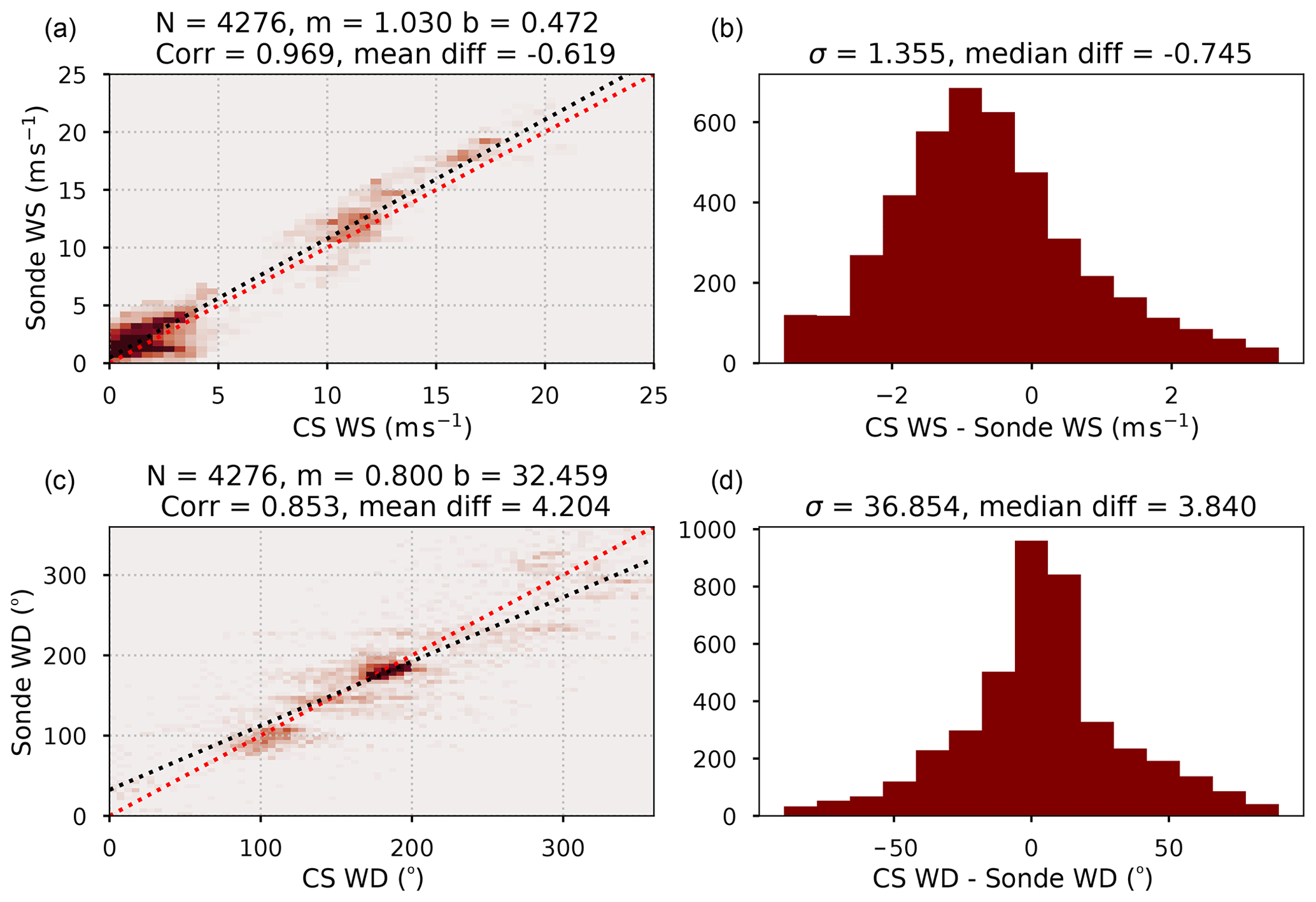
Figure 7Similar to Fig. 4 but comparing kinematic measurements from the radiosondes and the CopterSonde.
4.1.2 Radiosonde vs. CopterSonde
Figure 7 shows the wind speeds estimated by the radiosonde compared to the CopterSonde estimate. The wind speeds have a high correlation of 0.969 and a relatively low standard deviation of 1.355 m s−1. The same bias in wind speed presented in Sect. 4.1.1 is also seen here, indicating the CopterSonde is consistently underestimating the wind speed by approximately 0.75 m s−1. Possible reasons for this bias are discussed in Sect. 5.
The wind direction from the two systems has a lower correlation (0.853). While the wind directions observed generally agree well (mean difference of 4.204∘), there is a large standard deviation (36.854∘). Much of this noise results from the low wind speed observations from LAPSE-RATE; both the radiosonde and CopterSonde struggle to capture the correct wind direction when wind speeds are low (Fig. 6b).
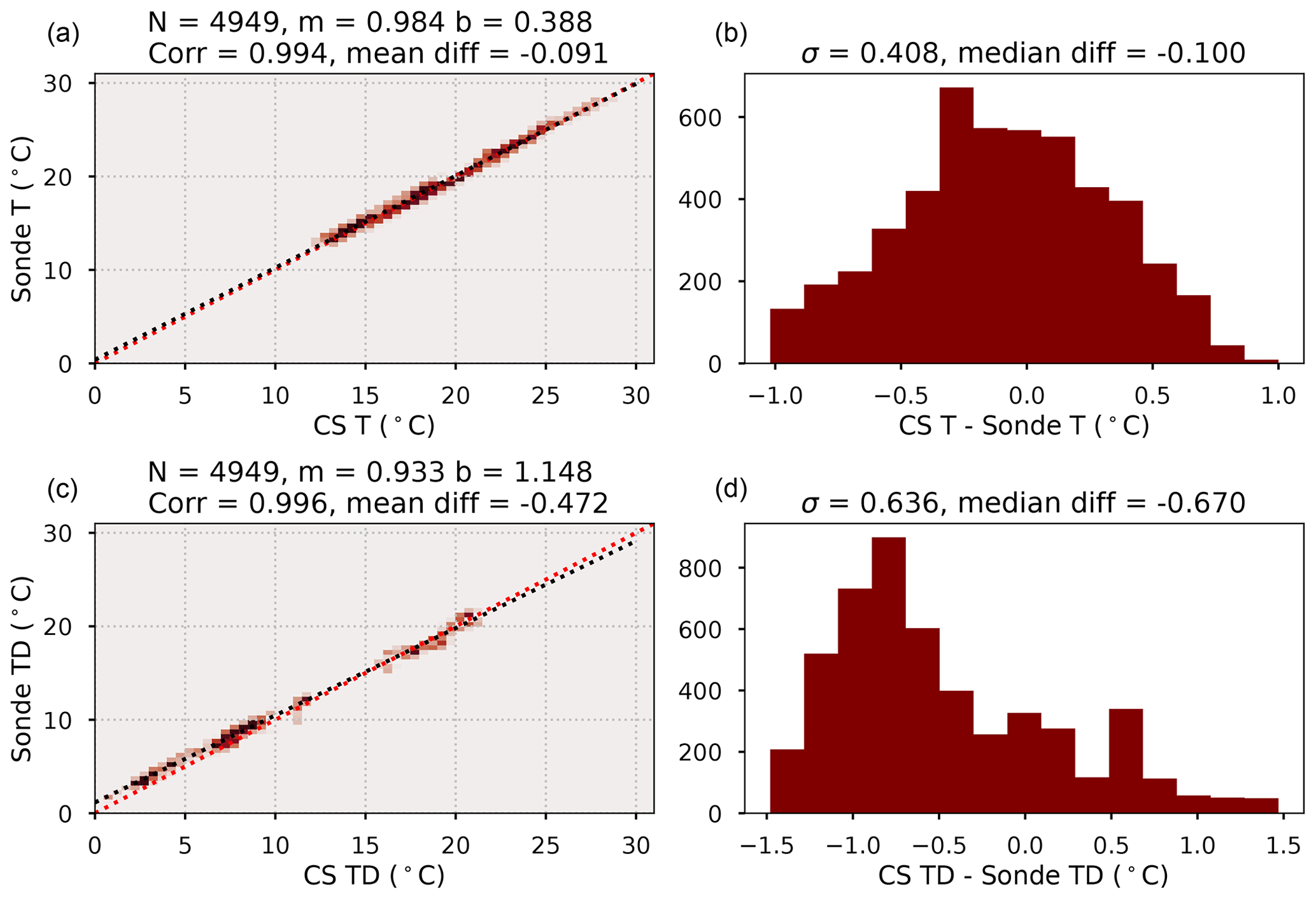
The radiosonde and CopterSonde data have a high level of agreement between their thermodynamic measurements. The correlation of the temperature and dew point temperature are both 0.99 (Fig. 8). The temperature comparison is slightly better, evidenced by the lower standard deviation (0.408 ∘C) and mean difference (−0.091 ∘C). A bias is observed in dew point temperatures lower than 13 ∘C. This grouping of measurements is entirely from the LAPSE-RATE campaign and there is a consistent offset. Given the CopterSonde was calibrated in a lab setting, while the radiosondes were not, this could be a moist bias on the part of the radiosondes. However, this has not been documented to the knowledge of the authors. It could also be the relative humidity sensors have a pressure dependence. Given the AERI moisture retrievals contained a high amount of spread compared to these instruments, it is difficult to determine which system is causing the bias.
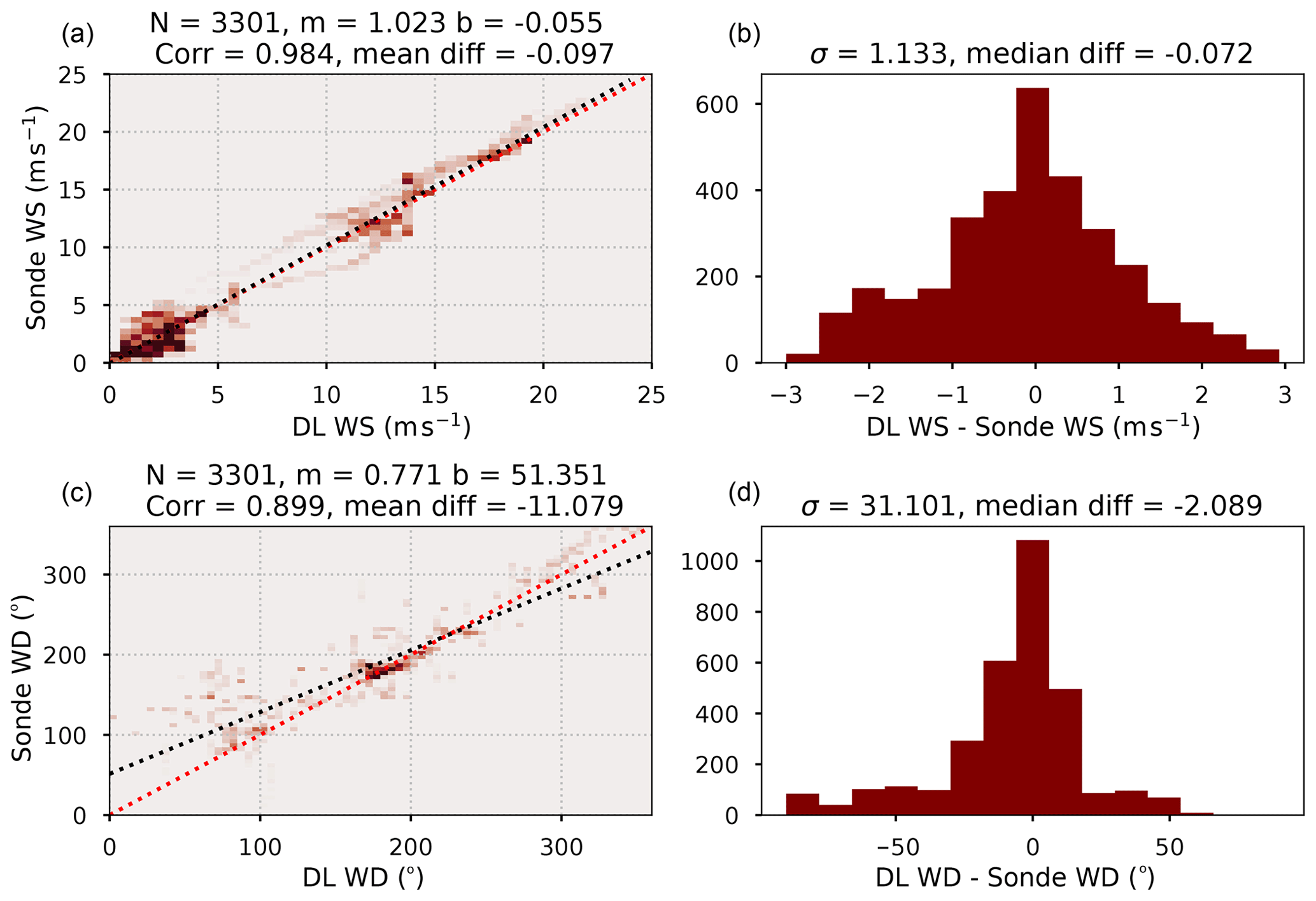
Figure 9Similar to Fig. 4 but comparing kinematic measurements from the radiosondes and the AERI.
4.1.3 Radiosonde vs. CLAMPS
Finally, Figs. 9 and 10 show comparisons between radiosondes and CLAMPS. The kinematic measurements from radiosondes and the DL compare well with a correlation of 0.984 for wind speed and 0.899 for wind direction (Fig. 9). There appears to be more noise in the wind directions, corresponding to a mean difference of −11.079∘. This is primarily from the low wind speeds observed during LAPSE-RATE, where all the systems have difficulty in accurately capturing the wind speed and direction (Fig. 6). There is a slight wind speed bias in one of the instruments, especially at higher wind speeds. However, since the CopterSonde shows bias in Sect. 4.1.1 and 4.1.2, it is impossible to determine which instrument has biased measurements. These results are similar to the results of Päschke et al. (2015), in particular the better performance at higher wind speeds.
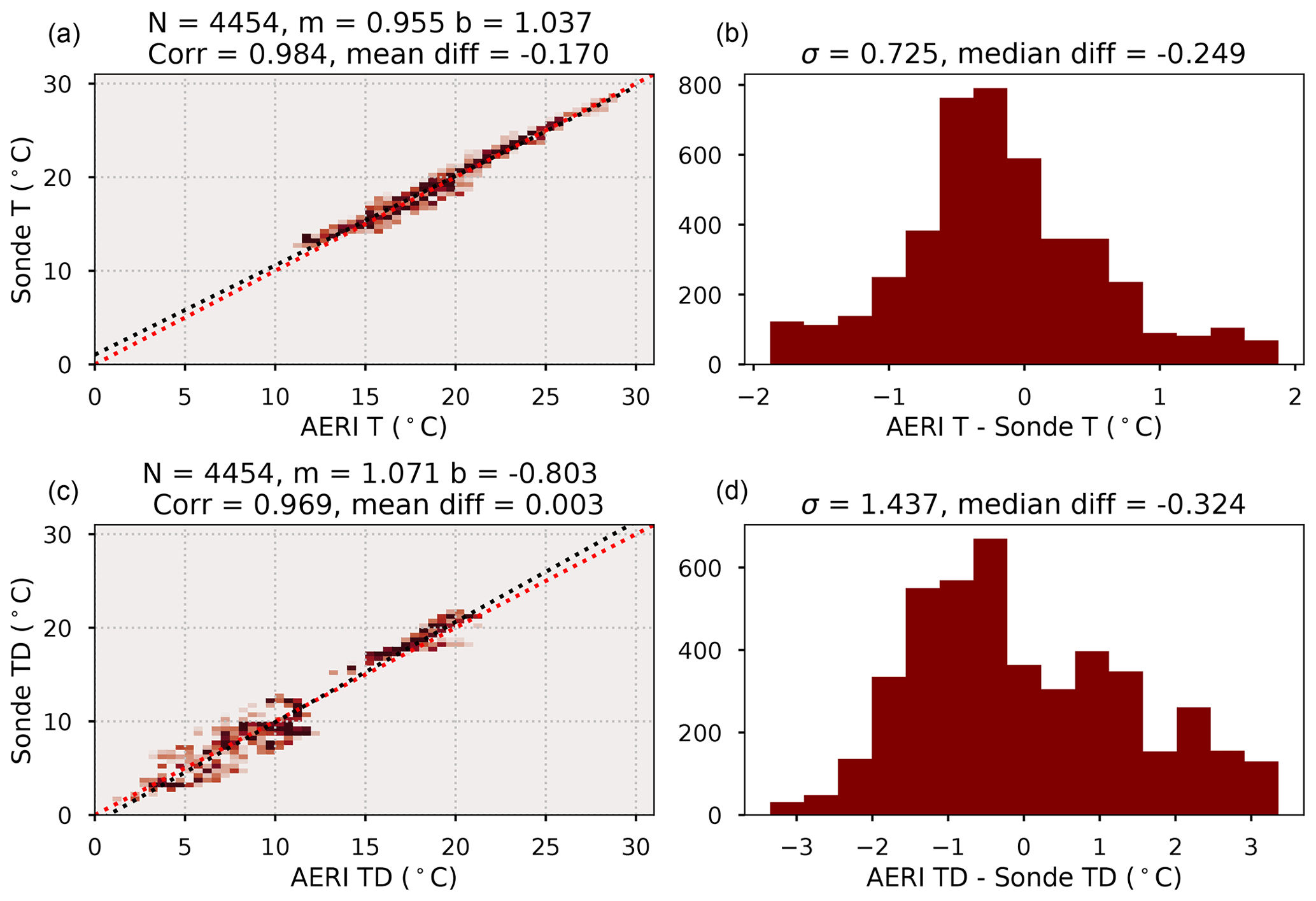
Figure 10 shows the thermodynamic comparisons between radiosondes and the AERI retrievals. These observations have a high correlation of 0.98 and a mean difference of −0.17 ∘C for temperature. The median difference is 0.249 and 0.324 ∘C for temperature and dew point temperature, respectively. These results also agree with past comparisons of AERIoe retrievals to radiosondes (Blumberg et al., 2015; Turner and Blumberg, 2018), namely the temperature retrieval tends to perform better (in terms of uncertainty) than the moisture retrieval.
4.2 Case studies
It is meaningful to analyze a couple of case studies in order to better understand how various features observed in the statistical analysis manifest themselves in individual profiles. Case studies also provide a sense of the conditions observed during the campaigns. A representative case from both Flux Capacitor and LAPSE-RATE will be shown to illustrate the different conditions observed.
4.2.1 LAPSE-RATE Case Study
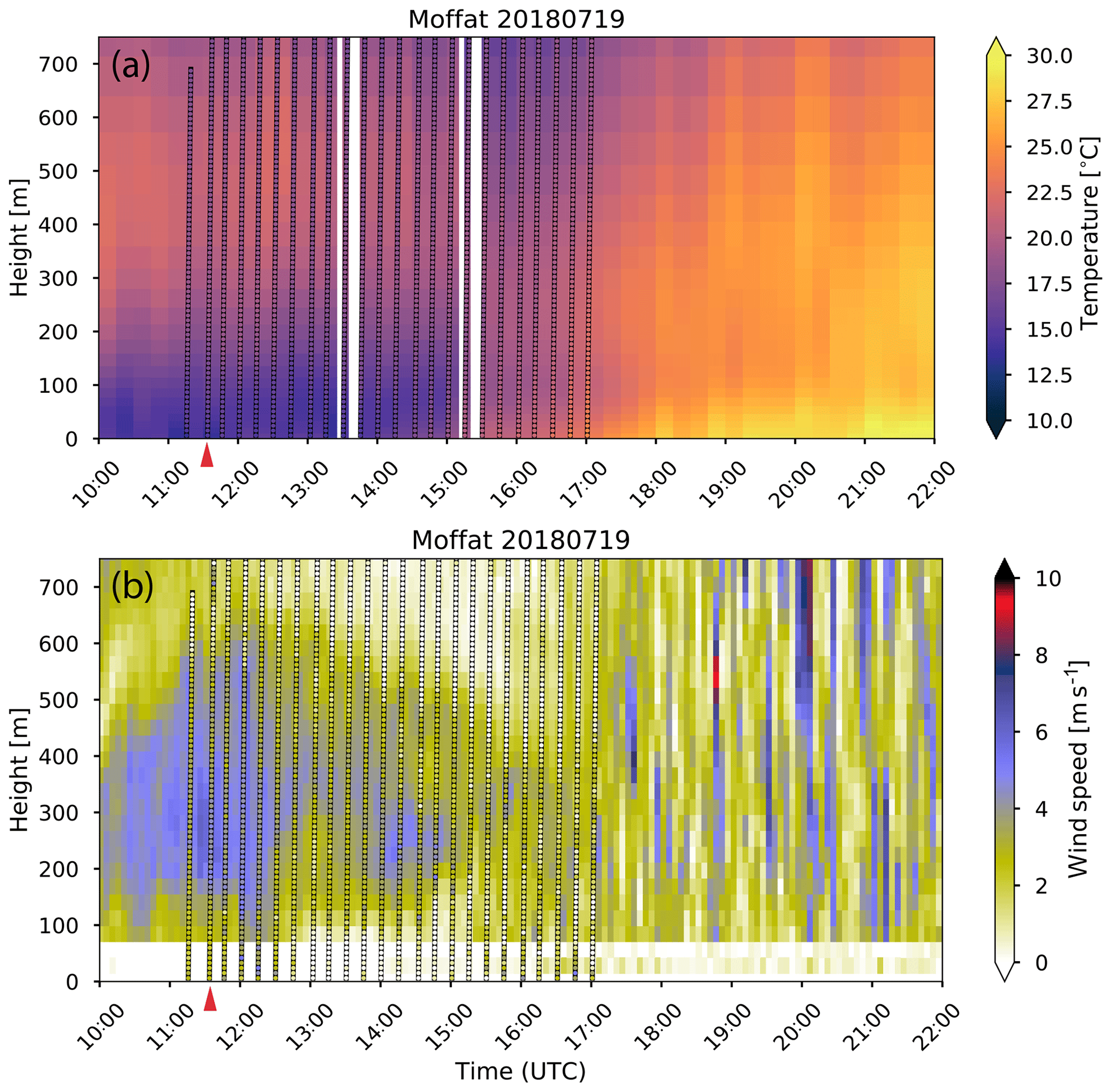
Figure 11Time–height plots of temperature (a) and wind speed (b) from the Moffat site on 19 July 2018. The background is temperature from the AERI retrievals, while the points overlaid on top are data from the CopterSonde at approximately 9 m resolution. The red arrow points to the profile shown in Fig. 12.
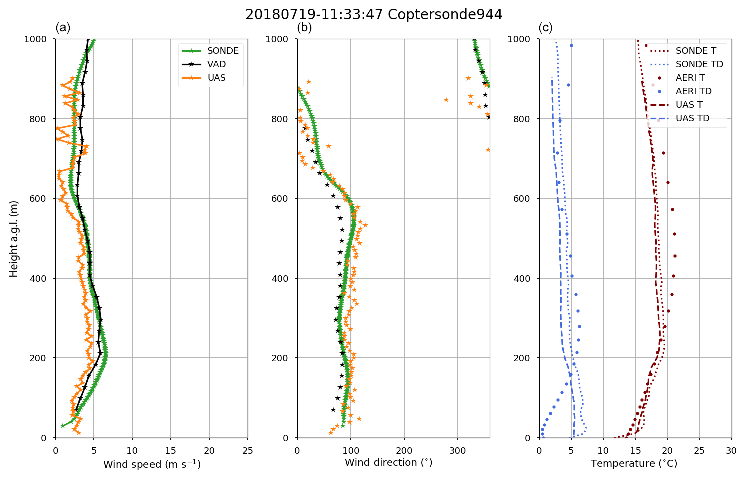
Figure 12Profile plots of wind speed (a), wind direction (b), and temperature and dew point temperature (c) from CLAMPS, the CopterSonde, and a radiosonde on 19 July 2018 at 11:33 UTC. The CopterSonde was launched just after the radiosonde, as soon as it was deemed the radiosonde was not in the flight path of the CopterSonde.
The first case considered is for 19 July 2018. During this period, the focus of LAPSE-RATE participants was to capture drainage flows in the northwestern part of the valley. CLAMPS and one of the CopterSonde teams continued to operate at the Moffat site during this period. Figure 11 shows the temperatures and wind speeds observed by CLAMPS and the CopterSonde at the Moffat site during this period. Flights started shortly after 11:00 UTC while there was still a strong nocturnal temperature inversion present and continued until 17:00 UTC. During this period, some of the highest wind speeds observed during LAPSE-RATE occurred.
Examining an example profile reveals some of the features presented in the statistical analysis. The wind speeds generally all fall within 2 m s−1 of each other, with the CopterSonde wind speed estimates generally tending to be the lowest (Fig. 12a). In terms of wind direction, the instruments all follow the same general pattern with height and are generally within 20∘ of each other (Fig. 12b). There is a wind speed maximum around 200 m a.g.l., likely due to the drainage flows from the surrounding mountains. The directional shear layer starting at approximately 600 m a.g.l. also indicates the presence of a slope flow.
The thermodynamic comparison between the AERI, CopterSonde, and radiosonde is shown in Fig. 12c. As would be expected, a nocturnal inversion is present. While all the systems capture the inversion, they are slightly different. The AERI retrieval smooths out the temperature inversion and shows the maximum temperature to be higher both in elevation and temperature than both the UAS and the radiosonde. This is a common occurrence in the data from the LAPSE-RATE campaign and may be due to the prior dataset that was used to generate the initial guess for the LAPSE-RATE retrievals, as mentioned in Sect. 4.1.1.
Additionally, there is a consistent offset between dew point temperatures measured by the CopterSonde and the radiosondes, which is observed throughout the LAPSE-RATE campaign. This is discussed in more detail in Sect. 5. In addition, AERI moisture retrieval performs poorly close to the surface. This could be due to a bad surface constraint.
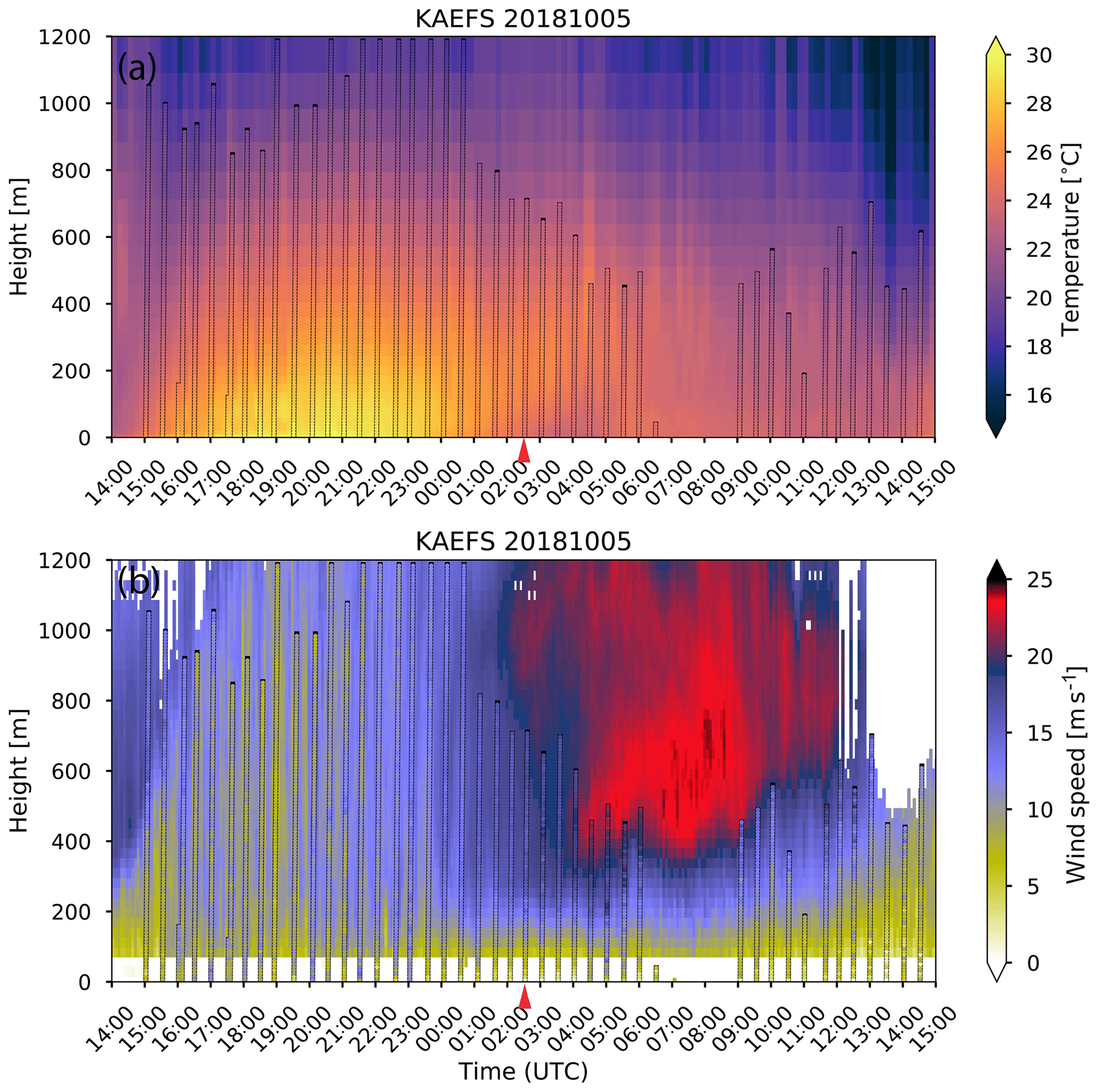
Figure 13Same as Fig. 11 but for 5–6 October 2018 during the Flux Capacitor campaign. These time heights contain data from the entire observation period.
4.2.2 Flux Capacitor case
The next case considered is from the OU-organized Flux Capacitor campaign in October 2018 (Fig. 13). During the overnight hours of Flux Capacitor, wind speeds were much higher than the LAPSE-RATE case due to the onset of a nocturnal low-level jet (LLJ, Fig. 13b). This is a common nighttime feature for the Southern Plains, and thus it is important to characterize how the CopterSonde performs in these high winds if a 3D Mesonet is to be established.
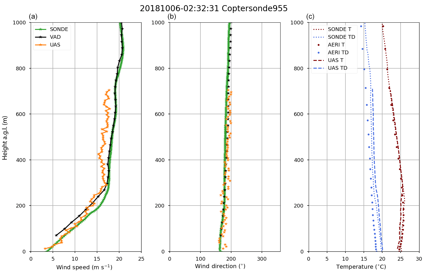
Figure 14 shows observations from the three systems on 6 October 2018 at 02:32 UTC. During this time period, wind speeds attained a maximum speed of 20 m s−1 around 850 m a.g.l. Due to the high winds, the flight was terminated before reaching 1200 m; this is one of the limitations of the CopterSonde. The CopterSonde also slightly underestimates the wind speed compared to the other systems once the vertical shear decreases. This could be due to the CopterSonde being calibrated for wind while it is stationary, rather than while it is ascending. It could also simply be that the calibration coefficients for wind speed are not valid for such high velocities. More investigation is needed in this area.
The thermodynamic data from the systems deployed during Flux Capacitor are in better agreement than the data presented in Sect. 4.2.1. All instruments are able to capture the nocturnal temperature inversion and accurately capture the residual layer. The difference in dew point temperature between the radiosonde and the CopterSonde is much smaller and the instruments agree well. The dew point temperature from the AERI has a slight bias but captures the general shape of the profile much better.
Overall, the systems tested all perform reasonably well when compared to each other. There are still many nuances to each instrument that need to be taken into account when deciding which system to use operationally. Additionally, some of the systems still need further development in select areas to insure good data quality.
For example, the CopterSonde currently underestimates the wind speed at higher velocities. This could be due to a number of factors. One likely possibility is that coefficients utilized to estimate the wind speed with the tilt of the craft are not valid at higher wind speeds. The coefficients used here were determined while loitering next to a 10 m tower at KAEFS while the wind speeds were generally less than 10 m s−1. Additionally, a linear relationship was used to determine these coefficients. As wind speeds increase, the CopterSonde must tilt more to compensate, leading to a larger cross-sectional area and thus more drag. This could lead to a nonlinear relationship that must be accounted for. Another possible reason for the underestimation is how the profile is performed. As mentioned before, the CopterSonde wind coefficients were determined while hovering at a constant altitude, but for these tests the CopterSonde was ascending at 3 m s−1. This could lead to a discrepancy in the observations since the pitch of the craft is likely different while ascending. Further experiments are being conducted to account for and correct the root cause of the wind speed underestimation.
In terms of thermodynamic measurements, all of the platforms were highly correlated with one another in temperature and dew point temperature. The AERIoe retrievals still need to be refined and there are a number of items that could have contributed to the spread, especially in the moisture fields from LAPSE-RATE. One of the major issues with the AERIoe retrievals from LAPSE-RATE is the proximity to the a priori dataset used to initially constrain the retrieval. Since there is no long-term archive of radiosondes launched in the San Luis Valley, radiosondes launched from the NWS office in Boulder, CO were used, which is over 200 km away. Additionally, uncertainty in the moisture retrievals are inherently larger for the conditions observed during LAPSE-RATE.
Due to these uncertainties in the AERIoe retrievals, it is difficult to determine whether the radiosonde or the CopterSonde exhibited biased moisture measurements during LAPSE-RATE. Since the CopterSonde sensors were well characterized in the Oklahoma Mesonet's calibration laboratory, it seems unlikely the bias could be from the CopterSonde. However, there could be a previously unknown pressure dependence in the sensors being used on the CopterSonde. More work is needed to determine the issue.
This study also highlights synergies between the various systems. For example, Doppler lidars and WxUAS can accurately capture full thermodynamic and kinematic profile at a resolution of 15–30 m, which is better than the specifications laid out by Hoff and Hardesty (2012).
Table 2Summary of CopterSonde measurement specifications based on the results of this study when compared to the Vaisala RS92-SGP data used in this study.
For meteorologists to fully take advantage of advanced high-resolution forecast models, high-resolution observations of the boundary layer are crucial. Two paradigms have been introduced to fill the current observational gap in the boundary layer. In this paper, data from WxUAS (the CopterSonde) and a system of atmospheric profiles (CLAMPS) were compared to the historical profiling standard, the radiosonde, during two different field campaigns.
In this study we found that all the systems agree relatively well, with correlations between all the instruments and variables greater than 0.85, with most above 0.90. The thermodynamic retrievals from CLAMPS perform well in terms of temperature, though the moisture retrievals could be improved. Additionally, there is still improvement to be made in wind speed estimation on the CopterSonde, mainly related to calibration procedures.
This study presents the most comprehensive comparison of a WxUAS to other profiling systems known to the authors. Additionally, it shows that measurements from WxUAS are comparable to other prominent profiling systems, and thus they can provide a low-cost alternative to expensive ground-based remote sensing systems for the 3D Mesonet concept laid out by Chilson et al. (2019). While the remote sensors and radiosondes presented in this study have been characterized by previous studies, the CopterSonde is a relatively new platform. Thus, we present specifications of the uncertainty in CopterSonde measurements when statistically compared to the RS92-SGP in Table 2. These were determined from the standard deviations of the differences calculated in this study. Note that the wind speed and direction uncertainties were determined using data with wind speeds greater than 4 m s−1.
Remote sensing systems will still have a place where WxUAS may not be able to fly, such as near busy airports or in incredibly remote locations where servicing WxUAS would be difficult. Future work will revolve around eliminating the bias from the CopterSonde wind measurements and using UAS to help retrieve other variables from the AERI, such as trace gases.
Data from the Flux Capacitor campaign are available upon request to the corresponding author. Data from LAPSE-RATE are publicly available on the data-hosting website Zenodo. The references for each dataset are as follows: CLAMPS Doppler lidar (Bell and Klein, 2020, https://doi.org/10.5281/zenodo.3780623), CLAMPS MWR and surface observations (Bell et al., 2020b, https://doi.org/10.5281/zenodo.3780593), AERIoe retrievals (Bell et al., 2020a, https://doi.org/10.5281/zenodo.3727224), CLAMPS radiosondes (Waugh, 2020, https://doi.org/10.5281/zenodo.3720444), and CopterSonde profiles (Greene et al., 2020, https://doi.org/10.5281/zenodo.3737087).
TMB and BRG were in charge of conceptualization. TMB, BRG, and PBC were in charge of the methodology. TMB developed the software, performed the formal analysis, created visualizations, and wrote the original draft. TMB, BRG, PMK, MC, and PBC assisted in the investigation. BRG, PMK, MC, and PBC assisted in the review and editing. PBC and PMK supervised and acquired the funding to perform the project.
The authors declare that they have no conflict of interest.
The authors would like to thank David Turner for his assistance in getting AERIoe running for the AERI retrievals in this paper. Additionally, the authors would like to thank Sean Waugh for his assistance in transporting CLAMPS to Colorado for LAPSE-RATE. This research has been supported in part by internal funding from the University of Oklahoma.
This research has been supported by the National Science Foundation, Office of Integrative Activities (grant no. 1539070).
This paper was edited by Jorge Luis Chau and reviewed by two anonymous referees.
Balsley, B. B., Lawrence, D. A., Woodman, R. F., and Fritts, D. C.: Fine-Scale Characteristics of Temperature, Wind, and Turbulence in the Lower Atmosphere (0–1300 m) Over the South Peruvian Coast, Bound.-Lay. Meteorol., 147, 165–178, 2013. a
Barbieri, L., Kral, S. T., Bailey, S. C., Frazier, A. E., Jacob, J. D., Reuder, J., Brus, D., Chilson, P. B., Crick, C., Detweiler, C., Doddi, A., Elston, J., Foroutan, H., González-Rocha, J., Greene, B. R., Guzman, M. I., Houston, A. L., Islam, A., Kemppinen, O., Lawrence, D., Pillar-Little, E. A., Ross, S. D., Sama, M. P., Schmale, D. G., Schuyler, T. J., Shankar, A., Smith, S. W., Waugh, S., Dixon, C., Borenstein, S., and de Boer, G.: Intercomparison of small unmanned aircraft system (sUAS) measurements for atmospheric science during the LAPSE-RATE campaign, Sensors, 19, 2179, https://doi.org/10.3390/s19092179, 2019. a, b
Båserud, L., Reuder, J., Jonassen, M. O., Kral, S. T., Paskyabi, M. B., and Lothon, M.: Proof of concept for turbulence measurements with the RPAS SUMO during the BLLAST campaign, Atmos. Meas. Tech., 9, 4901–4913, https://doi.org/10.5194/amt-9-4901-2016, 2016. a
Bell, T. and Klein, P.: OU/NSSL CLAMPS Doppler Lidar Data from LAPSE-RATE, Zenodo, https://doi.org/10.5281/zenodo.3780623, 2020. a
Bell, T., Klein, P., and Turner, D.: OU/NSSL CLAMPS AERIoe Temperature and Water Vapor Profile Data from LAPSE-RATE, Zenodo, https://doi.org/10.5281/zenodo.3727224, 2020a. a
Bell, T., Klein, P., and Turner, D.: OU/NSSL CLAMPS Microwave Radiometer and Surface Meteorological Data from LAPSE-RATE, Zenodo, https://doi.org/10.5281/zenodo.3780593, 2020b. a
Bessagnet, B., Menut, L., Couvidat, F., Meleux, F., Siour, G., and Mailler, S.: What Can We Expect from Data Assimilation for Air Quality Forecast? Part II: Analysis with a Semi-Real Case, J. Atmos. Ocean. Tech., 36, 1433–1448, https://doi.org/10.1175/JTECH-D-18-0117.1, 2019. a
Blumberg, W. G., Turner, D. D., Löhnert, U., and Castleberry, S.: Ground-Based Temperature and Humidity Profiling Using Spectral Infrared and Microwave Observations. Part II: Actual Retrieval Performance in Clear-Sky and Cloudy Conditions, J. Appl. Meteorol. Clim., 54, 2305–2319, 2015. a, b
Bonin, T., Chilson, P., Zielke, B., and Fedorovich, E.: Observations of the Early Evening Boundary-Layer Transition Using a Small Unmanned Aerial System, Bound.-Lay. Meteorol., 146, 119–132, https://doi.org/10.1007/s10546-012-9760-3, 2012. a
Browning, K. A. and Wexler, R.: The Determination of Kinematic Properties of a Wind Field Using Doppler Radar, J. Appl. Meteorol., 7, 105–113, 1968. a
Chilson, P., Gleason, A., Zielke, B., Nai, F., Yeary, M., Klein, P., and Shalamunec, W.: SMARTSonde: A small UAS platform to support radar research, AMS 34th Conf. Radar Meteor., Boston, 8 October 2009, MA. Am. Meteorol. Soc., 2009. a
Chilson, P. B., Bell, T. M., Brewster, K. A., Britto Hupsel de Azevedo, G., Carr, F. H., Carson, K., Doyle, W., Fiebrich, C. A., Greene, B. R., Grimsley, J. L., Kanneganti, S. T., Martin, J., Moore, A., Palmer, R. D., Pillar-Little, E. A., Salazar-Cerreno, J. L., Segales, A. R., Weber, M. E., Yeary, M., and Droegemeier, K. K.: Moving towards a Network of Autonomous UAS Atmospheric Profiling Stations for Observations in the Earth’s Lower Atmosphere: The 3D Mesonet Concept, Sensors, 19, 2720, https://doi.org/10.3390/s19122720, 2019. a, b
de Boer, G., Palo, S., Argrow, B., LoDolce, G., Mack, J., Gao, R.-S., Telg, H., Trussel, C., Fromm, J., Long, C. N., Bland, G., Maslanik, J., Schmid, B., and Hock, T.: The Pilatus unmanned aircraft system for lower atmospheric research, Atmos. Meas. Tech., 9, 1845–1857, https://doi.org/10.5194/amt-9-1845-2016, 2016. a
de Boer, G., Diehl, C., Jacob, J., Houston, A., Smith, S. W., Chilson, P., III, D. G. S., Intrieri, J., Pinto, J., Elston, J., Brus, D., Kemppinen, O., Clark, A., Lawrence, D., Bailey, S. C., Sama, M. P., Frazier, A., Crick, C., Natalie, V., Pillar-Little, E., Klein, P., Waugh, S., Lundquist, J. K., Barbieri, L., Kral, S. T., Jensen, A. A., Dixon, C., Borenstein, S., Hesselius, D., Human, K., Hall, P., Argrow, B., Thornberry, T., Wright, R., and Kelly, J. T.: Development of community, capabilities and understanding through unmanned aircraft-based atmospheric research: The LAPSE-RATE campaign, B. Am. Meteorol. Soc., 101, E684–E699, https://doi.org/10.1175/BAMS-D-19-0050.1, 2020. a
Geerts, B., Raymond, D. J., Grubišić, V., Davis, C. A., Barth, M. C., Detwiler, A., Klein, P. M., Lee, W.-C., Markowski, P. M., Mullendore, G. L., and Moore, J. A.: Recommendations for In Situ and Remote Sensing Capabilities in Atmospheric Convection and Turbulence, B. Am. Meteorol. Soc., 99, 2463–2470, 2018. a
Gioli, B., Miglietta, F., Vaccari, F. P., Zaldei, A., and De Martino, B.: The Sky Arrow ERA, an innovative airborne platform to monitor mass, momentum and energy exchange of ecosystems, Ann. Geophys., 49, https://doi.org/10.4401/ag-3159, 2006. a
Greene, B., Segales, A., Bell, T., Pillar-Little, E., and Chilson, P.: Environmental and Sensor Integration Influences on Temperature Measurements by Rotary-Wing Unmanned Aircraft Systems, Sensors, 19, 1470, https://doi.org/10.3390/s19061470, 2019. a, b, c, d
Greene, B. R., Segales, A. R., Waugh, S., Duthoit, S., and Chilson, P. B.: Considerations for temperature sensor placement on rotary-wing unmanned aircraft systems, Atmos. Meas. Tech., 11, 5519–5530, https://doi.org/10.5194/amt-11-5519-2018, 2018. a, b, c
Greene, B. R., Bell, T. M., Pillar-Little, E. A., Segales, A. R., Britto Hupsel de Azevedo, G., Doyle, W., Tripp, D. D., Kanneganti, S. T., and Chilson, P. B.: University of Oklahoma CopterSonde Files from LAPSE-RATE, Zenodo, https://doi.org/10.5281/zenodo.3737087, 2020. a
Hoff, R. M. and Hardesty, R. M.: Thermodynamic Profiling Technologies Workshop Report to the National Science Foundation and the National Weather Service, Tech. rep., National Center for Atmospheric Research, 2012. a, b, c
Houston, A. L., Argrow, B., Elston, J., Lahowetz, J., Frew, E. W., and Kennedy, P. C.: The Collaborative Colorado–Nebraska Unmanned Aircraft System Experiment, B. Am. Meteorol. Soc., 93, 39–54, 2012. a
Hubbard, K., Lin, X., Baker, C., and Sun, B.: Air temperature comparison between the MMTS and the USCRN temperature systems, J. Atmos. Ocean. Tech., 21, 1590–1597, https://doi.org/10.1175/1520-0426(2004)021<1590:ATCBTM>2.0.CO;2, 2004. a
Hunter, J. D.: Matplotlib: A 2D graphics environment, Comput. Sci. Eng., 9, 90–95, https://doi.org/10.1109/MCSE.2007.55, 2007. a
Knuteson, R. O., Revercomb, H. E., Best, F. A., Ciganovich, N. C., Dedecker, R. G., Dirkx, T. P., Ellington, S. C., Feltz, W. F., Garcia, R. K., Howell, H. B., Smith, W. L., Short, J. F., and Tobin, D. C.: Atmospheric Emitted Radiance Interferometer. Part I: Instrument Design, J. Atmos. Ocean. Tech., 21, 1763–1776, 2004a. a
Knuteson, R. O., Revercomb, H. E., Best, F. A., Ciganovich, N. C., Dedecker, R. G., Dirkx, T. P., Ellington, S. C., Feltz, W. F., Garcia, R. K., Howell, H. B., Smith, W. L., Short, J. F., and Tobin, D. C.: Atmospheric Emitted Radiance Interferometer. Part II: Instrument Performance, J. Atmos. Ocean. Tech., 21, 1777–1789, 2004b. a
Koch, S. E., Fengler, M., Chilson, P. B., Elmore, K. L., Argrow, B., Andra, D. L., and Lindley, T.: On the Use of Unmanned Aircraft for Sampling Mesoscale Phenomena in the Preconvective Boundary Layer, J. Atmos. Ocean. Tech., 35, 2265–2288, 2018. a, b, c, d, e
Kral, S. T., Reuder, J., Vihma, T., Suomi, I., Oâ'Connor, E., Kouznetsov, R., Wrenger, B., Rautenberg, A., Urbancic, G., Jonassen, M. O., BÃserud, L., Maronga, B., Mayer, S., Lorenz, T., Holtslag, A. A. M., Steeneveld, G.-J., Seidl, A., Müller, M., Lindenberg, C., Langohr, C., Voss, H., Bange, J., Hundhausen, M., Hilsheimer, P., and Schygulla, M.: Innovative Strategies for Observations in the Arctic Atmospheric Boundary Layer (ISOBAR) – The Hailuoto 2017 Campaign, Atmosphere, 9, 268, https://doi.org/10.3390/atmos9070268, 2018. a
Lawrence, D. A. and Balsley, B. B.: High-Resolution Atmospheric Sensing of Multiple Atmospheric Variables Using the DataHawk Small Airborne Measurement System, J. Atmos. Ocean. Tech., 30, 2352–2366, 2013. a
Lothon, M., Lohou, F., Pino, D., Couvreux, F., Pardyjak, E. R., Reuder, J., Vilà-Guerau de Arellano, J., Durand, P., Hartogensis, O., Legain, D., Augustin, P., Gioli, B., Lenschow, D. H., Faloona, I., Yagüe, C., Alexander, D. C., Angevine, W. M., Bargain, E., Barrié, J., Bazile, E., Bezombes, Y., Blay-Carreras, E., van de Boer, A., Boichard, J. L., Bourdon, A., Butet, A., Campistron, B., de Coster, O., Cuxart, J., Dabas, A., Darbieu, C., Deboudt, K., Delbarre, H., Derrien, S., Flament, P., Fourmentin, M., Garai, A., Gibert, F., Graf, A., Groebner, J., Guichard, F., Jiménez, M. A., Jonassen, M., van den Kroonenberg, A., Magliulo, V., Martin, S., Martinez, D., Mastrorillo, L., Moene, A. F., Molinos, F., Moulin, E., Pietersen, H. P., Piguet, B., Pique, E., Román-Cascón, C., Rufin-Soler, C., Saïd, F., Sastre-Marugán, M., Seity, Y., Steeneveld, G. J., Toscano, P., Traullé, O., Tzanos, D., Wacker, S., Wildmann, N., and Zaldei, A.: The BLLAST field experiment: Boundary-Layer Late Afternoon and Sunset Turbulence, Atmos. Chem. Phys., 14, 10931–10960, https://doi.org/10.5194/acp-14-10931-2014, 2014. a
Markowski, P. M.: An Idealized Numerical Simulation Investigation of the Effects of Surface Drag on the Development of Near-Surface Vertical Vorticity in Supercell Thunderstorms, J. Atmos. Sci., 73, 4349–4385, https://doi.org/10.1175/JAS-D-16-0150.1, 2016. a
Markowski, P. M. and Bryan, G. H.: LES of Laminar Flow in the PBL: A Potential Problem for Convective Storm Simulations, Mon. Weather Rev., 144, 1841–1850, https://doi.org/10.1175/MWR-D-15-0439.1, 2016. a
National Academies of Sciences, Engineering and Medicine: Thriving on Our Changing Planet: A Decadal Strategy for Earth Observation from Space, The National Academies Press, Washington, DC, 2018. a
National Research Council: Observing Weather and Climate from the Ground Up: A Nationwide Network of Networks, The National Academies Press, Washington, DC, 2009. a, b
Neumann, P. P. and Bartholmai, M.: Real-time wind estimation on a micro unmanned aerial vehicle using its inertial measurement unit, Sensor. Actuat. A-Phys., 235, 300–310, 2015. a
Nowotarski, C. J., Markowski, P. M., and Richardson, Y. P.: The Characteristics of Numerically Simulated Supercell Storms Situated over Statically Stable Boundary Layers, Mon. Weather Rev., 139, 3139–3162, https://doi.org/10.1175/MWR-D-10-05087.1, 2011. a
Park, S.-Y., Kim, D.-H., Lee, S.-H., and Lee, H. W.: Variational data assimilation for the optimized ozone initial state and the short-time forecasting, Atmos. Chem. Phys., 16, 3631–3649, https://doi.org/10.5194/acp-16-3631-2016, 2016. a
Päschke, E., Leinweber, R., and Lehmann, V.: An assessment of the performance of a 1.5 μm Doppler lidar for operational vertical wind profiling based on a 1-year trial, Atmos. Meas. Tech., 8, 2251–2266, https://doi.org/10.5194/amt-8-2251-2015, 2015. a, b, c
Pearson, G., Davies, F., and Collier, C.: An Analysis of the Performance of the UFAM Pulsed Doppler Lidar for Observing the Boundary Layer, J. Atmos. Ocean. Tech., 26, 240–250, 2009. a, b
Pedregosa, F., Varoquaux, G., Gramfort, A., Michel, V., Thirion, B., Grisel, O., Blondel, M., Prettenhofer, P., Weiss, R., Dubourg, V., Vanderplas, J., Passos, A., Cournapeau, D., Brucher, M., Perrot, M., and Duchesnay, E.: Scikit-learn: Machine Learning in Python, J. Mach. Learn. Res., 12, 2825–2830, 2011. a
Reuder, J., Brisset, P., Jonassen, M., Müller, M., and Mayer, S.: The Small Unmanned Meteorological Observer SUMO: A new tool for atmospheric boundary layer research, Meteorol. Z., 18, 141–147, 2009. a
Reuder, J., Jonassen, M. O., and Ólafsson, H.: The Small Unmanned Meteorological Observer SUMO: Recent developments and applications of a micro-UAS for atmospheric boundary layer research, Acta Geophys., 60, 1454–1473, 2012. a
Rodgers, C. D.: Inverse methods for atmospheric sounding: Theory and practice, vol. 2 of Series on Atmospheric, Oceanic, and Planetary Physics, World Scientific, 2000. a
Rose, T., Crewell, S., Löhnert, U., and Simmer, C.: A network suitable microwave radiometer for operational monitoring of the cloudy atmosphere, Atmos. Res., 75, 183–200, https://doi.org/10.1016/j.atmosres.2004.12.005, 2005. a
Saïd, F., Corsmeier, U., Kalthoff, N., Kottmeier, C., Lothon, M., Wieser, A., Hofherr, T., and Perros, P.: ESCOMPTE experiment: intercomparison of four aircraft dynamical, thermodynamical, radiation and chemical measurements, Atmos. Res., 74, 217–252, https://doi.org/10.1016/j.atmosres.2004.06.012, 2005. a
Segales, A. R., Greene, B. R., Bell, T. M., Doyle, W., Martin, J. J., Pillar-Little, E. A., and Chilson, P. B.: The CopterSonde: an insight into the development of a smart unmanned aircraft system for atmospheric boundary layer research, Atmos. Meas. Tech., 13, 2833–2848, https://doi.org/10.5194/amt-13-2833-2020, 2020. a
Tanner, B. D., Swiatek, E., and Maughan, C.: Field comparisons of naturally ventilated and aspirated radiation shields for weather station air temperature measurements, in: Conference on Agricultural and Forest Meteorology, 22, 227–230, 1996. a
Turner, D. D. and Blumberg, W. G.: Improvements to the AERIoe Thermodynamic Profile Retrieval Algorithm, IEEE Journal of Selected Topics in Applied Earth Observations and Remote Sensing, 1–16, 2018. a, b, c
Turner, D. D. and Löhnert, U.: Information Content and Uncertainties in Thermodynamic Profiles and Liquid Cloud Properties Retrieved from the Ground-Based Atmospheric Emitted Radiance Interferometer (AERI), J. Appl. Meteorol. Clim., 53, 752–771, 2014. a, b, c
van den Kroonenberg, A. C., Martin, S., Beyrich, F., and Bange, J.: Spatially-averaged temperature structure parameter over a heterogeneous surface measured by an unmanned aerial vehicle, Bound.-Lay. Meteorol., 142, 55–77, https://doi.org/10.1007/s10546-011-9662-9, 2012. a
van der Walt, S., Colbert, S. C., and Varoquaux, G.: The NumPy Array: A Structure for Efficient Numerical Computation, Comput. Sci. Eng., 13, 22–30, https://doi.org/10.1109/MCSE.2011.37, 2011. a
Virtanen, P., Gommers, R., Oliphant, T. E., Haberland, M., Reddy, T., Cournapeau, D., Burovski, E., Peterson, P., Weckesser, W., Bright, J., van der Walt, S. J., Brett, M., Wilson, J., Jarrod Millman, K., Mayorov, N., Nelson, A. R. J., Jones, E., Kern, R., Larson, E., Carey, C., Polat, İ., Feng, Y., Moore, E. W., VanderPlas, J., Laxalde, D., Perktold, J., Cimrman, R., Henriksen, I., Quintero, E. A., Harris, C. R., Archibald, A. M., Ribeiro, A. H., Pedregosa, F., and van Mulbregt, P.: SciPy 1.0–Fundamental Algorithms for Scientific Computing in Python, arXiv [preprint], arXiv:1907.10121, 23 July 2019. a
Vömel, H., Argrow, B. M., Axisa, D., Chilson, P., Ellis, S., Fladeland, M., Frew, E. W., Jacob, J., Lord, M., Moore, J., Oncley, S., Roberts, G., Schoenung, S., and Wolff, C.: The NCAR / EOL Community Workshop on Unmanned Aircraft Systems for Atmospheric Research, UCAR/NCAR Earth Observing Laboratory, 2018. a
Wagner, T. J., Klein, P. M., and Turner, D. D.: A New Generation of Ground-Based Mobile Platforms for Active and Passive Profiling of the Boundary Layer, B. Am. Meteorol. Soc., 100, 137–153, 2019. a
Waugh, S.: National Severe Storms Laboratory Mobile Soundings during Lapse-Rate (CLAMPS trailer), Zenodo, https://doi.org/10.5281/zenodo.3720444, 2020. a
Wildmann, N., Hofsäß, M., Weimer, F., Joos, A., and Bange, J.: MASC-a small remotely piloted aircraft (RPA) for wind energy research, Adv. Sci. Res., 11, 55, https://doi.org/10.5194/asr-11-55-2014, 2014. a
Wildmann, N., Rau, G. A., and Bange, J.: Observations of the Early Morning Boundary-Layer Transition with Small Remotely-Piloted Aircraft, Bound.-Lay. Meteorol., 157, 345–373, 2015. a
World Health Organization: Ambient air pollution: a global assessment of exposure and burden of disease, 2016. a
Zhou, B. and Chow, F. K.: Turbulence Modeling for the Stable Atmospheric Boundary Layer and Implications for Wind Energy, Flow Turbul. Combust., 88, 255–277, https://doi.org/10.1007/s10494-011-9359-7, 2012. a